An exactly solvable system from quantum optics

Abstract

We investigate a generalisation of the Rabi system in the Bargmann-Fock representation. In this representation the eigenproblem of the considered quantum model is described by a system of two linear differential equations with one independent variable. The system has only one irregular singular point at infinity. We show how the quantisation of the model is related to asymptotic behaviour of solutions in a vicinity of this point. The explicit formulae for the spectrum and eigenfunctions of the model follow from an analysis of the Stokes phenomenon. An interpretation of the obtained results in terms of differential Galois group of the system is also given.

I Introduction and results

In paper Maciejewski:14::a we proposed a general method which allows to determine spectra of quantum systems given in the Bargmann representation. This representation is very useful for systems with a Hilbert space which is a product of a finite and infinite-dimensional spaces. A typical example is a Hamiltonian for spin degrees of freedom of some particles, characterised by $n$-dimensional $\sigma$ matrices, coupled to a bosonic field via annihilation and creation operators $a$, and $a^{{\dagger}}$. Then $n$-component wave function $\psi=(\psi_{1},\ldots,\psi_{n})$ is an element of Hilbert space $\mathscr{H}^{n}=\mathscr{H}\times\cdots\times\mathscr{H}$, where $\mathscr{H}$ is the Bargmann-Fock Hilbert space of entire functions. The scalar product in $\mathscr{H}$ is given by

$$\langle f,g\rangle=\dfrac{1}{\pi}\int_{\mathbb{C}}\overline{f(z)}g(z)\mathrm{e}^{-|z|^{2}}\,\mathrm{d}x\,\mathrm{d}y,\quad z=x+\mathrm{i}\,y.$$

Since operators $a$ and $a^{{\dagger}}$ are represented by $\partial_{z}$ and multiplication by $z$, respectively, for clearly $[\partial_{z},z]=1$, stationary Schrödinger equation $H\psi=E\psi$ becomes the system of linear ordinary differential equations. Usually such systems have a certain number of regular singular points in the complex $z$ plane, and possibly an irregular point at infinity. Determination of the spectrum consists in finding such values of $E$ that all the components of wave function $\psi_{i}$, with $i=1,\ldots,n$, are elements of the Hilbert space $\mathscr{H}$.

In paper Maciejewski:14::a we have shown that a solution of the eigenvalue problem can be reduced to checking the following three conditions.

1. Local conditions. At each regular singular point $z=s$ there exists at least one solution which is holomorphic in an open set containing $s$.

2. Global conditions. At each singular point we can select a local holomorphic solution in such a way that they are analytic continuations of each other. That is, they are local representations of an entire solution.

3. Normalisation conditions. The entire solution selected above must have a finite Bargmann norm.

The first two conditions were analysed in detail in Maciejewski:14::a and in Maciejewski:14:: we gave their effective application for determination of full spectrum of the Rabi system.

The third condition is highly non-trivial. This is so because “most” of entire functions do not belong to $\mathscr{H}$. In order to analyse this condition we need to characterise the growth of an entire solution $f(z)$ of a system of linear differential equations. In a neighbourhood of a regular singular point the growth of $f(z)$ is polynomial. Hence, if the considered system has only regular singular points, and $f(z)$ is its entire solution, then $f(z)$ has a finite Bargmann norm. Normalisation conditions can give non-trivial constrains on entire solution only if the linear system has an irregular singularity, for example at infinity.

The growth of entire function $f(z)$ is described by means of the following function:

$$M(r):=\underset{|z|=r}{\mathrm{max}}|f(z)|.$$ (1)

It is used to define two numbers which characterise properties of the growth. The order, or the growth order $\varrho$ of $f(z)$ is defined as the limit

$$\varrho:=\lim_{r\rightarrow\infty}\sup\frac{\ln(\ln M(r))}{\ln r},\quad\mathrm{with}\quad 0\leq\varrho\leq\infty.$$ (2)

For an entire function of finite order $\varrho<\infty$, its type $\sigma$ is defined as

$$\sigma:=\lim_{r\rightarrow\infty}\sup\frac{\ln M(r)}{r^{\varrho}}.$$ (3)

If $f(z)$ belongs to $\mathscr{H}$, then one can prove the following facts Bargmann:61:: :

1. $f(z)$ is of order $\varrho\leq 2$.

2. If $\varrho=2$, then $f(z)$ is of type $\sigma\leq\tfrac{1}{2}$.

If $\varrho=2$ and $\sigma=\tfrac{1}{2}$, then the question whether $f(z)\in\mathscr{H}$ requires a separate investigation. For additional details see Vourdas:06:: .

It is well known that in a neighbourhood of a regular singular point, a formal procedure allows to find formal series which satisfy the equation. It appears that this formal series is convergent, so it is a local solution of the equation. In a vicinity of irregular singular point a formal procedure gives formal expressions which satisfy the equation, however the series are generally divergent. It is known that these formal expressions, give the asymptotic expansion of a solution valid in in certain sectors radially extending from the vertex localised at this singularity. Borders of sectors are determined by the so-called Stokes lines. The asymptotic expansions change when we pass from one sector to another. These changes are governed by the so-called Stokes matrices.

The normalisation condition of an entire solution $f(z)$ implies that at each sector $S$ the following integral

$$\int_{S}|f(z)|^{2}\mathrm{e}^{-|z|^{2}}\,\mathrm{d}x\,\mathrm{d}y,$$ (4)

has a finite value. Thus, at each sector it has good asymptotics which guarantees the convergence of the above integral. This implies that although a solution $f(z)$ can change its asymptotic expansion from sector to sector, these changes are restricted only to good asymptotics. This property implies that all Stokes matrices have a common invariant subspace, in particular case just one common eigenvector.

The aim of this paper is to show that the above considerations can be applied effectively. We consider system given by the following Hamiltonian

$$H=\left(\omega+\dfrac{U}{2}\sigma_{z}\right)a^{{\dagger}}a+\dfrac{\omega_{0}}{2}\sigma_{z}+g\sigma_{x}(a^{{\dagger}}+a),$$ (5)

where $\sigma_{x}$, $\sigma_{z}$ are the Pauli spin matrices and $\omega_{0}$, $\omega$, $g$ and $U$ are parameters. For $U=0$, it coincides with the Hamiltonian of the Rabi model Rabi:36:: describing interaction of a two-level atom with a single harmonic mode of the electromagnetic field. Hamiltonian (5) was proposed in Grimsmo:13::a ; Grimsmo:14::a . The term $\frac{U}{2}\sigma_{z}a^{{\dagger}}a$ can be interpreted as a nonlinear coupling between the atom and the cavity.

In Bargmann-Fock representation, the stationary Schrödinger equation $H\psi=E\psi$, with $\psi=(\psi_{1},\psi_{2})$, have the form

$$\begin{split}\left(\omega+\dfrac{U}{2}\right)z\psi_{1}^{\prime}+\dfrac{\omega_{0}}{2}\psi_{1}+g\psi_{2}^{\prime}+gz\psi_{2}=E\psi_{1},\\ \left(\omega-\dfrac{U}{2}\right)z\psi_{2}^{\prime}-\dfrac{\omega_{0}}{2}\psi_{2}+g\psi_{1}^{\prime}+gz\psi_{1}=E\psi_{2}.\end{split}$$ (6)

In our paper Maciejewski:14::a we calculated the spectrum of $H$ for the generic case, i.e., when the above system has two regular singular points. This requires that $U^{2}\neq 4\omega^{2}$, and the quantisation of the energy spectrum results from the condition that system (6) admits an entire solution. In that case, all entire solutions of (6) have a finite norm.

In this paper we investigate the remaining cases for which $U^{2}=4\omega^{2}$. For $U=+2\omega$ system (6) can be rewritten in the form

$$\begin{split}\psi_{1}^{\prime}(z)=&-z\psi_{1}(z)+\frac{2E+\omega_{0}}{2g}\psi_{2}(z),\\ \psi_{2}^{\prime}(z)=&\frac{4\omega z^{2}+2E-\omega_{0}}{2g}\psi_{1}(z)-\\ &\frac{z\left[g^{2}+\omega(2E+\omega_{0})\right]}{g^{2}}\psi_{2}(z).\end{split}$$ (7)

The system for the case of $U=-2\omega$ can be obtained from the above equations by a simple change $\omega_{0}\rightarrow-\omega_{0}$, and the interchange $\psi_{1}$ with $\psi_{2}$. Hence, we consider only the case $U=+2\omega$.

System (7) has no singular points in the finite part of $\mathbb{C}$, so all its solutions are entire functions. Infinity is the only and irregular singular point. The system can have solutions which grow fast enough to make the Bargmann norm infinite. Thus, to determine the spectrum of the problem we have to find all values of $E$ for which system admits a solution with a moderate growth at infinity, such that its Bargmann norm is finite.

We give a full answer to this question. That is we specify explicitly a countable number of energy values for which the corresponding eigenfunctions are also given explicitly and have a finite Bargmann norm.

The energy axis is divided into two disjoint intervals, each of them with its own countable family of eigenvalues. To be more precise, our main result is as follows. Let

$$x:=1+\omega g^{-2}(E+\omega_{0}/2),$$ (8)

be an auxiliary spectral parameter. Then the Hamiltonian (5) has entire solutions with a finite Bargmann norm if and only if one of the following conditions is fulfilled. Either $x>1$, and

$$\frac{(x-1)\left(\omega(\omega-\omega_{0})+g^{2}(x-1)\right)}{\omega^{2}\sqrt{x^{2}-1}}=2n+1,$$ (9)

or $x<-1$, and

$$\frac{(x-1)\left(\omega(\omega-\omega_{0})+g^{2}(x-1)\right)}{\omega^{2}\sqrt{x^{2}-1}}=-(2n+1),$$ (10)

where $n\in\mathbb{N}$. The respective eigenfunctions

$$\psi^{\pm}_{n}=\left(\psi_{1,n}^{\pm},\psi_{2,n}^{\pm}\right),$$

are given by

$$\begin{split}\psi_{1,n}^{\pm}(z)&=C\exp\left(-\beta_{\pm}z^{2}\right)H_{n}\left(\sqrt{\pm 1}\sqrt[4]{x^{2}-1}\,z\right),\\ \psi_{2,n}^{\pm}(z)&=\frac{\omega}{g(x-1)}\left[\psi_{1,n}^{\pm}(z)+\left(\psi_{1,n}^{\pm}(z)\right)^{\prime}\right],\end{split}$$ (11)

where $H_{n}(z)$ denotes the Hermite polynomial of degree $n$, and

$$\beta_{\pm}:=\frac{x\pm\sqrt{x^{2}-1}}{2}.$$

These functions have the growth order $\varrho=2$ and type $\sigma=\beta_{\pm}$.

II Asymptotic expansions

An asymptotic expansion of a function $\psi(z)$ for $z\rightarrow\infty$ is denoted in the following way

$$\psi(z)\sim a_{0}+\frac{a_{1}}{z}+\frac{a_{2}}{z^{2}}+\ldots\,.$$ (12)

By definition it means that in a given sector

$$S(a,b):=\{z\in\mathbb{C}\,|\,a<\arg(z)<b,\quad|z|>r_{0}\},$$

we have

$$\lim_{z\rightarrow\infty}\left(\psi(z)-\sum_{j=0}^{m}a_{j}z^{-j}\right)z^{m}=0,$$ (13)

for an arbitrary $m\in\mathbb{N}$, and $z\in S(a,b)$. Such series needs not have a positive radius of convergence.

Note that if

$$\psi(z)e^{-P(z)}\sim a_{0}+\mathcal{O}(z^{-1}),$$ (14)

for a certain function $P(z)$, then, in particular

$$\lim_{z\rightarrow\infty}\psi(z)e^{-P(z)}=a_{0},$$ (15)

and $|\psi(z)|=\mathcal{O}(\exp|P(z)|)$.

The general form of solutions around irregular singular points is known, and there are several classical theorems on them. We choose two, particularly suitable here, namely Theorems 12.3 and 19.1 given in Wasow:87:: , which tell as the following.

Let us suppose that the system in question can be written as

$$z^{-q}\psi^{\prime}(z)=A(z)\psi(z),\qquad\psi(z)\in\mathbb{C}^{n},$$ (16)

where $A(z)$ is $n\times n$ matrix holomorphic in a neighbourhood of infinity and $A_{0}:=A(\infty)$ is nonzero. Then in every sufficiently narrow sector $S$, the equation has a fundamental matrix of solutions of the form

$${\Psi}(z)=Y(z)z^{G}e^{Q(z)},$$ (17)

where $G$ is a constant $n\times n$ matrix, $Q(z)$ is a diagonal matrix whose elements are polynomials of $z^{1/p}$ with a suitable positive integer $p$, and $Y(z)$ admits an asymptotic power series in $z^{-1/p}$. If we further assume that the eigenvalues $\lambda_{i}$ of $A_{0}$, are all distinct, then

• $G$ is a diagonal matrix,

• $p=1$ and $Q(z)$ is also diagonal with leading terms of $\lambda_{i}z^{q+1}/(q+1)$,

• $S$ can be any sector of central angle not exceeding $\pi/(q+1)$.

The fact that asymptotic expansions are unique allows for their formal calculation, and the above tells us, that there are always solutions which grow according to the prescribed formal expressions. The problem is that for a true (not just formal) solution the asymptotic behaviour changes from sector to sector—only in rare cases are the expansions valid for all values of the argument.

It can be shown, see Wasow:87:: , that if a function is single valued near infinity, its asymptotic expansion is valid for all values of $\arg(z)$ if and only if it is analytic at $z=\infty$ and the series is actually convergent .

In our case the requirement of finite Bargmann norm is that

$$|\psi(z)|=\mathcal{O}\left(e^{\sigma|z|^{\varrho}}\right),\quad\varrho\leq 2,$$ (18)

and $|\sigma|\leq\tfrac{1}{2}$ when $\varrho=2$. So the determination of the exponential factor will be crucial, and we shall see that the considered model presents us with functions of growth order $\varrho=2$ and varying types $\sigma$, which require detailed analysis.

III Spectrum determination

In the case $U=+2\omega$ the considered model is described by (7). This system has the standard form (16) with $q=2$. Since the leading matrix $A_{0}$ is nilpotent, it is convenient to perform a shearing transform

$$\psi_{i}(z)=z^{i-1}\xi_{i}(z),\quad i=1,2,$$ (19)

after which the system becomes

$$\frac{1}{z}\boldsymbol{\xi}^{\prime}(z)=\begin{bmatrix}-1&(x-1)\frac{g}{\omega}\\ \frac{2\omega}{g}+\frac{g^{2}(x-1)-\omega\omega_{0}}{g\omega z^{2}}&1-2x-\frac{1}{z^{2}}\end{bmatrix}\boldsymbol{\xi}(z),$$ (20)

where $\boldsymbol{\xi}=[\xi_{1},\xi_{2}]^{T}$, $x$ is a new spectral parameter defined by (8). The rank of the system is thus $q+1=2$, and the matrix $A_{0}$ has eigenvalues $x\pm\sqrt{x^{2}-1}$. We can immediately discard the case of them being equal, for then, the system (7) is explicitly solvable. For example, when $x=1$ we have

$$\psi_{1}(z)=c_{1}e^{-z^{2}/2},\,\,\psi_{2}(z)=\frac{c_{2}}{3g}e^{-z^{2}/2}(2\omega z^{3}-3\omega_{0}z),$$

and these functions have infinite Bargmann norm.

We are thus left only with the simpler case of two distinct eigenvalues and we know what form of asymptotic expansions to expect. Following Birkhoff Birkhoff:1909:: , let us assume the following Laplace integral representation for the vector of solutions

$$\psi_{i}(z)=\frac{1}{2\pi\mathrm{i}}\int_{C}\exp(z^{2}y)(\eta_{0,i}(y)+z\eta_{1,i}(y))\mathrm{d}y,$$ (21)

where $i=1,2$. The usual inverse Laplace transform would be

$$\frac{1}{2\pi\mathrm{i}}\int_{C}\exp(zy)\eta(y)\text{d}y,$$ (22)

However, such $\eta$ would, in general, have essential singularities in the finite complex plane because we are dealing with an equation of rank 2. To remedy this, the exponential part needs to be modified in anticipation of the growth order 2. This procedure is applicable whenever the matrix $A_{0}$ has different eigenvalues, regardless of the rank of the equation, for further details see Birkhoff:1909:: .

The contour of integration $C$ is chosen so that the integrand assumes the same value at both ends. It could be a loop or an open contour extending to infinity. Here, the latter is more viable, and $C$ will be one of the curves shown in Figure 1. This will allow to integrate by parts as follows

$$\int_{C}\exp(z^{2}y)z^{n}u(y)\mathrm{d}y=\\ \left[\exp(z^{2}y)z^{n-2}u(y)\right]_{C}-\int_{C}\exp(z^{2}y)z^{n-2}u^{\prime}(y)\mathrm{d}y,$$ (23)

and taking the bracket term to be zero. Substituting the Laplace representation (21) in equation (7) we obtain a new system for $(\eta_{0,i},\eta_{1,i})$ with $i=1,2$, by equating the integrands to zero. That this is permissible can be checked later where the particular $\eta$ are recovered but we are mostly interested in the asymptotic expansions in which case the expressions obtained will be formal anyway.

The integrands are polynomials of $z$ and integrating by parts as in (23) we can reduce their degree to at most 1. Then the coefficients of $z^{0}$ and $z^{1}$ must each be zero so that we end up with a system of four equations

$$\begin{split}\omega\eta_{11}+g(x-1)\eta_{02}+\omega(2y+1)\eta_{11}^{\prime}&=0,\\ \omega(2y+1)\eta_{01}-g(x-1)\eta_{12}&=0,\\ \omega(2\omega\eta_{01}^{\prime}-g(2y+2x-1)\eta_{12}^{\prime}-g\eta_{12})&\\ +(\omega_{0}\omega-g^{2}(x-1))\eta_{01}&=0,\\ (\omega_{0}\omega-g^{2}(x-1))\eta_{11}+&\\ \omega(2\omega\eta_{11}^{\prime}+g(2y+2x-1)\eta_{02})&=0,\end{split}$$ (24)

where prime denotes differentiation with respect to $y$. First two equations can be immediately solved for two components

$$\begin{split}\eta_{02}&=-\frac{\omega}{g(x-1)}\left((2y+1)\eta_{11}^{\prime}+\eta_{11}\right),\\ \eta_{12}&=\frac{\omega(2y+1)}{g(x-1)}\eta_{01}.\end{split}$$ (25)

This leaves two first order equations for the remaining components

$$\begin{split}(4y^{2}+4xy+1)\eta_{10}^{\prime}&=\left(4\rho\sqrt{x^{2}-1}-6y-3x\right)\eta_{10},\\ (4y^{2}+4xy+1)\eta_{11}^{\prime}&=\left(4\rho\sqrt{x^{2}-1}-2y-x\right)\eta_{11},\\ \end{split}$$ (26)

where

$$\rho=-\frac{(x-1)\left(\omega(\omega-\omega_{0})+g^{2}(x-1)\right)}{4\omega^{2}\sqrt{x^{2}-1}}.$$ (27)

Although the particular equations decouple, this is obviously not a generic feature. It makes sense then to treat them as a system with two regular singular points at

$$\alpha_{1,2}=\frac{1}{2}\left(-x\pm\sqrt{x^{2}-1}\right),$$ (28)

and one at infinity. The characteristic exponents are

$$\begin{split}\beta_{1}\in\left\{\rho-\tfrac{3}{4},\rho-\tfrac{1}{4}\right\}\quad&\text{at }\alpha_{1},\\ \beta_{2}\in\left\{-\rho-\tfrac{3}{4},-\rho-\tfrac{1}{4}\right\}\quad&\text{at }\alpha_{2},\\ \beta_{\infty}\in\left\{\tfrac{3}{2},\tfrac{1}{2}\right\}\quad&\text{at }\infty.\end{split}$$ (29)

In general, the behaviour of a solution as it is continued around all the singular points cannot be specified explicitly as the monodromy group of the equation is unknown. Fortunately, solutions of system (LABEL:decoup) are given explicitly

$$\begin{split}\eta_{01}&=b_{1}(y-\alpha_{1})^{\rho-3/4}(y-\alpha_{2})^{-\rho-3/4},\\ \eta_{11}&=b_{2}(y-\alpha_{1})^{\rho-1/4}(y-\alpha_{2})^{-\rho-1/4},\end{split}$$ (30)

where $b_{1,2}$ are arbitrary constants. The explicit forms of these solutions will give us full information about which contours to choose and how the continuation of any solution behaves.

Each singular point of the solution $\eta_{i,j}(y)$ corresponds to a different exponential factor in the asymptotic expansion, which can be seen as follows. Let us look at the generic case first, when the contour can be chosen as path $C_{i}$ that runs from infinity to the vicinity of the point $y=\alpha_{i}$, around it in the positive direction, then back to infinity, as depicted in Figure 1.

Figure 1: Contours. $\alpha_{1}=\delta=1/(4\alpha_{2})$

This requires that the characteristic exponent at that singularity $\alpha_{i}$ is not an integer, for otherwise the integral vanishes. Since, for the system (LABEL:decoup) for all singular points the differences of exponents is $1/2$, one solution is always suitable.

The Laplace integral (21) for any function $\eta(y)$ which has a local power series around $y=\alpha$ with characteristic exponent $\beta$ may be rewritten as

$$\frac{e^{\alpha z^{2}}}{2\pi\mathrm{i}}\int_{C}e^{z^{2}(y-\alpha)}(y-\alpha)^{\beta}\sum_{n=0}^{\infty}a_{n}(y-\alpha)^{n}\mathrm{d}y\\ =\frac{e^{\alpha z^{2}}}{z^{2(\beta+1)}}\sum_{n=0}^{\infty}\frac{a_{n}}{\Gamma(-\beta-n)z^{2n}},$$ (31)

where we have used the integral representation of the gamma function, and omitted indices for brevity. The series is not, in general, convergent in the whole complex plane of $y$, so the integration term by term using the gamma function leads to a formal, divergent in most cases, asymptotic expansion. It can be shown that this is the correct asymptotic series Kohno:99:: , so that it is immediately evident that each singular point $\alpha_{i}$ gives rise to one type of exponential factor $\exp(\alpha_{i}z^{2})$ in the asymptotic series. Note that $4\alpha_{1}\alpha_{2}=1$ and in view of the previous section we require $|\alpha_{i}|<1/2$, so only one of the contours will lead to the desired growth type. The special case of $|\alpha_{i}|=1/2$ will be dealt with separately, below.

It is important to keep in mind that the contour had to be chosen so that the integrand vanishes as $y\rightarrow\infty$ and that the integral (21) is convergent – this is ensured by $\text{Re}(z^{2}y)<0$. In other words, for a given argument of $z$ there is just a sector of the complex plane of $y$ where the integral converges and vice versa: for a given ray ($\arg(y-\alpha)$) in the $y$ plane, there is a region of convergence in the $z$ plane. An example is shown in Figure 2. Because the components $\eta$ grow at most with some power of $y$ at infinity, the integral (21) converges fast enough, for the function to be holomorphic and it is indeed permissible to differentiate it as we have done.

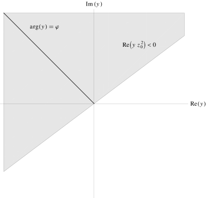
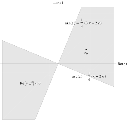
Figure 2: The corresponding sectors in the $y$ and $z$ planes for $z_{0}=1+\mathrm{i}/2$. Note that both shaded regions on the right fulfil $\text{Re}(yz^{2})<0$ for any given $y$ with $\arg(y)=\varphi$.

To extend the function outside one sector, the integral can be analytically continued by deforming the contour, rotating it around a given singularity. Because the contour has to pass through the other singularity, the solution associated with one asymptotics could transform into a combination of both, as shown in figure 3. This is the Stokes phenomenon, and the argument of $\alpha_{1}-\alpha_{2}$ determines the so-called Stokes lines in the $z$ plane, which is customarily given by the condition $\text{Re}(z^{2}(\alpha_{1}-\alpha_{2}))=0$; crossing the line causes the asymptotic expansions to mix. There is the freedom of choosing the starting contour, which corresponds to choosing a particular solution, and the first Stokes line where the deformation is required depends on that choice. But if we continue a full basis increasing the argument of $z$ we eventually need to take into account all of the lines. For the considered case, $\alpha_{1}-\alpha_{2}$ is real, so there are two Stokes lines which pass through the origin and form angles $\pm\pi/4$ with the $x$-axis.

Figure 3: Deformation.

Upon crossing, the original integral decomposes into integrals over new contours, which could be written shortly as

$$\mathcal{A}\int_{C_{i}}=\int_{C^{\prime}_{j}}+\,\int_{C^{\prime}_{i}}-\,e^{2\pi\mathrm{i}\beta_{i}}\int_{C^{\prime}_{j}},$$ (32)

where $\mathcal{A}$ stands for analytic continuation, and primes are used to distinguish between contours in the two regions: $\text{Im}(y)>0$ and $\text{Im}(y)<0$, although their shape remains the same. This could be written using the Stokes matrix as

$$\mathcal{A}(e_{i},e_{j})=(e^{\prime}_{i},e^{\prime}_{j})\begin{pmatrix}1&0\\ 1-e^{2\pi\mathrm{i}\beta_{i}}&1\end{pmatrix},$$ (33)

where $e_{i}$ is the solution obtained with $C_{i}$, hence with fixed asymptotics of $\exp(\alpha_{i}z^{2})$, and likewise for $e^{\prime}_{i}$ and $C^{\prime}_{i}$. By convention, the matrix on the right-hand side is the inverse of the Stokes matrix.

As $\beta_{i}$ is not an integer, whether the additional integral actually contributes, depends on the characteristic exponent of the solution around $\alpha_{j}$. If $\beta_{j}$ is not an integer either, the Stokes multiplier is obviously not zero. On the other hand, for an integer $\beta_{j}$ the contour $C_{j}$ can simply be deformed through the singularity so the integral is identically zero, because

$$\int_{C_{j}}=\left(1-e^{2\pi\mathrm{i}\beta_{j}}\right)\int_{\alpha_{j}}^{\infty}=:\left(1-e^{2\pi\mathrm{i}\beta_{j}}\right)\int_{L_{j}}.$$ (34)

This does not mean that the asymptotic solution $e_{j}$ vanishes, but simply that the contour $L_{j}$, which is a half line from $\alpha_{j}$ to infinity, has to be used instead of $C_{j}$ to define the other asymptotic solution $e_{j}$. The Stokes matrix is then

$$\mathcal{A}(e_{i},e_{j})=(e^{\prime}_{i},e^{\prime}_{j})\begin{pmatrix}1&0\\ 0&1\end{pmatrix}.$$ (35)

For completeness we note that the contour $L_{j}$ can be deformed analogously to the above, this time winding around $\alpha_{i}$. Because $\beta_{i}$ is not an integer, the contour cannot pass through the singular point and the additional path will be exactly $C_{i}$. In terms of the Stokes matrix we have

$$\mathcal{A}(e^{\prime}_{i},e^{\prime}_{j})=(e^{\prime\prime}_{i},e^{\prime\prime}_{j})\begin{pmatrix}1&1\\ 0&1\end{pmatrix}.$$ (36)

In other words, the asymptotics of the solution $e_{i}$ remains unchanged, while the asymptotic series $e_{j}$ actually exhibits the Stokes phenomenon because $\beta_{i}$ is not an integer. The double primes signify contours identical to the original ones for $\text{Im}(y)>0$ but the solutions are not single-valued in general so $e_{i}^{\prime\prime}$ are some multiples of $e_{i}$.

Note, that when $\beta_{j}$ is an integer, $\beta_{i}$ cannot be, since their sum is $-3/2$ or $-1/2$ for the two solutions of $\eqref{lapeq}$, respectively. Thus, the conditions that the contour is suited for the noninteger exponent at $\alpha_{i}$ and that the Stokes multiplier vanishes are consistent. There is no need then to investigate the case of integer $\beta_{i}$, because for any $\rho$ we always have at least one solution with noninteger exponent at each of the singular points. It follows that we always have two different solutions $e_{i}$ with different asymptotic expansions obtained by means of the contours $C$ and, as stated in the previous section, the fundamental solutions have to be expressible by means of those two $e_{i}$ in any sector. In each case then, we know how both asymptotic solutions mix when crossing the Stokes lines and hence, how the growth of any actual solution changes. For the system under consideration the situation is very simple, because only the asymptotic series with smaller $\alpha_{i}$ is suitable, so that all of its Stokes multipliers must be zero to ensure finite norm.

It remains to verify that when $x^{2}<1$ and hence $|\alpha_{i}|=1/2$ the resulting solutions are not normalisable, in close analogy to the $x=1$ case, where the components of the wave function behave like $e^{z^{2}/2}$. The exponential factor in the present case can be written as

$$\exp\left(\frac{1}{2}e^{\mathrm{i}\theta}z^{2}\right),\quad\text{for }\alpha_{j}=\frac{1}{2}e^{\mathrm{i}\theta_{j}},$$ (37)

and since the equation determining $\alpha_{j}$ is real we have $\alpha_{2}=\bar{\alpha_{1}}$ so $\theta_{2}=-\theta_{1}\neq 0$. Together with the Bargmann measure this results in the leading factor of the form

$$\int_{0}^{2\pi}\int_{0}^{\infty}\exp\left(-2r^{2}\sin^{2}\left(\varphi+\frac{\theta}{2}\right)\right)r\text{d}r\text{d}\varphi,$$ (38)

where we took $z=re^{\mathrm{i}\varphi}$. The integral over $r$ converges provided that the sine does not vanish, i.e. in sectors that do not include the directions $\varphi+\theta_{j}/2=k\pi$, $k\in\mathbb{Z}$. If there is no Stokes phenomenon for the solutions with asymptotic factors of $e^{\alpha_{i}z^{2}}$, it follows that the norm is not finite. If the two solutions could interchange, we would necessarily have to construct a solution which has the asymptotics of $\exp(\alpha_{1}z^{2})$ in the vicinity of $\varphi+\theta_{2}/2=0$. But then, continuing it through the angle of $\pi$ in $\arg(z)=\varphi$, we would end up in a sector containing the next problematic line $\varphi+\theta_{2}/2=\pi$. The corresponding contour in the $y$ plane would have to rotate through $2\pi$ and the Stokes phenomenon would cause the asymptotic expansion to now contain also the series with $\exp(\alpha_{2}z^{2})$ whose norm would diverge in the second sector. Thus regardless of the Stokes multipliers, although the solutions are both entire, none of them is normalisable for $-1\leq x\leq 1$. One could interpret this as a continuum spectrum with generalised eigenstates, because to each entire function in the Bargmann space corresponds a well behaved distribution solution of the original problem in the $L^{2}(\mathbb{R})$ space Bargmann:61:: .

Taking the above into account, we can finally give conditions for the original entire function to be normalisable. First, for the desired asymptotics one must have $|\alpha_{i}|<1/2$ so that the solution starts as normalisable within some Stokes sector, and second $\beta_{j}\in\mathbb{N}$, so that it remains such, as it is continued throughout the whole complex plane. The second condition is going to be of the form $\pm\rho-3/4\in\mathbb{N}$ or $\pm\rho-1/4\in\mathbb{N}$ as there are two solutions of (30) to choose from, but these can be written together as $\pm 4\rho=2n+1$, $n\in\mathbb{N}$.

Returning to the spectral parameter $x$, the normalisation, and quantisation, conditions read:

$$\left\{\begin{aligned} |\alpha_{1}|&<\frac{1}{2}\iff x>1,\\ -4\rho&=2n_{+}+1,\quad n_{+}\in\mathbb{N},\end{aligned}\right.$$ (39)

$$\left\{\begin{aligned} |\alpha_{2}|<\frac{1}{2}\iff x<-1,\\ 4\rho=2n_{-}+1,\quad n_{-}\in\mathbb{N}.\end{aligned}\right.$$ (40)

or, equivalently,

$$\mathrm{sgn}(x)\frac{(x-1)\left(\omega(\omega-\omega_{0})+g^{2}(x-1)\right)}{\omega^{2}\sqrt{x^{2}-1}}=2n+1,$$ (41)

for $x^{2}>1$ and $n\in\mathbb{N}$. The energies of these spectra are presented in Fig. 4 and 5; note that the lower levels become denser as $E$ gets closer to the continuous (non-normalisable) region $x^{2}<1$.

It is evident, that with these conditions there will always be one characteristic exponent that is a negative integer. In this case one of the contours $C$ will be equivalent to a circle and the corresponding Laplace integral can be immediately evaluated using Cauchy’s theorem. It will yield a finite number of terms so that the solution will be a polynomial in $z$ with an exponential factor. A change of variables then reveals that each interval of $x$ has its own sets of eigenstates expressible in terms of Hermite polynomials, namely

$$\psi_{1}(z)=c_{1}\exp\left(\frac{-x-\sqrt{x^{2}-1}}{2}z^{2}\right)H_{n_{-}}\left(\sqrt[4]{x^{2}-1}\,z\right),$$ (42)

when $x<-1$, or

$$\psi_{1}(z)=c_{2}\exp\left(\frac{-x+\sqrt{x^{2}-1}}{2}z^{2}\right)H_{n_{+}}\left(\mathrm{i}\sqrt[4]{x^{2}-1}\,z\right),$$ (43)

when $x>1$, and in each case the other component is

$$\psi_{2}(z)=\frac{\omega}{g(x-1)}\left(z\psi_{1}(z)+\psi_{1}^{\prime}(z)\right).$$ (44)

Figure 4: The upper spectrum for $\omega=1$ and $\omega_{0}=1/2$.

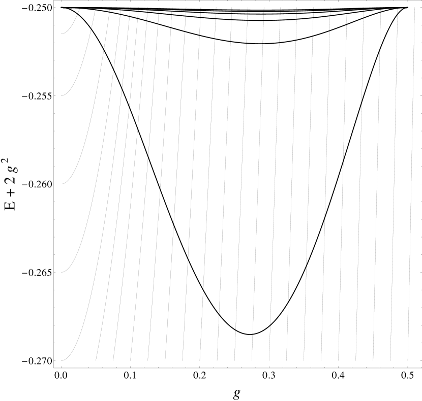
Figure 5: The lower spectrum for $\omega=1$ and $\omega_{0}=1/2$. Thin lines denote constant energy levels.

IV Connection with the Whittaker equation

Let us rewrite system (6) as one equation of the second order. It reads

$$w^{\prime\prime}+2xzw^{\prime}+\left(z^{2}+x-m\sqrt{x^{2}-1}\right)w=0,$$ (45)

where $w(z)=\psi_{1}(z)$, $x$ is defined by (8), and

$$m:=\frac{(x-1)\left[\omega(\omega-\omega_{0})+g^{2}(x-1)\right]}{\omega^{2}\sqrt{x^{2}-1}}.$$ (46)

Now, we introduce new independent variable $y$, and change the depended variable putting $y=z^{2}\sqrt{x^{2}-1}$ and

$$v(y)=y^{1/4}\exp\left[\frac{xy}{2\sqrt{x^{2}-1}}\right]w(z).$$ (47)

We obtain the Whittaker equation

$$v^{\prime\prime}(y)-\left(\frac{1}{4}-\frac{\kappa}{y}+\frac{4\mu^{2}-1}{y^{2}}\right)v(y)=0,$$ (48)

with parameters

$$\kappa=-\frac{1}{4}m,\qquad\mu=\frac{1}{4}.$$ (49)

According to Proposition 2.5 in Morales:99::c , there exists a basis of solutions of this equation such that two Stokes matrices have the form

$$S_{1}=\begin{bmatrix}1&\alpha\\ 0&1\end{bmatrix}\quad\text{and}\quad S_{2}=\begin{bmatrix}1&0\\ \beta&1\end{bmatrix},$$ (50)

where $\alpha$ and $\beta$ are some complex numbers. Moreover, the Stokes multiplier $\alpha$ vanishes if and only if either $\kappa+\mu$, or $\kappa-\mu$ is a non-negative half integer. Similarly, the Stokes multiplier $\beta$ vanishes if and only if either $-\kappa-\mu$, or $-\kappa+\mu$ is a non-negative half integer. The reader can check, that in the considered case these conditions exactly coincide with those given by (9) and (10).

Now, it is interesting to observe that for the Whittaker equation if one of the Stokes multipliers vanishes, then it is solvable in the sense of differential Galois theory—all its solutions are Liouvillian. More precisely, the identity component of its differential Galois group is Abelian, see Corollary 2.1 in Morales:99::c . We have the same conclusions for equation (45) describing our problem. Thus, if $E$ is an eigenvalue then:

1. A Stokes multiplier vanishes;

2. All solution are Liouvillian;

3. The identity component of its differential Galois group is solvable.

These observations are very important for application. If we are able to prove inverse implications, then we have a strong tool for quantisation and finding exactly solvable systems. In fact, for low order equations there exist effective algorithms for studying their differential Galois groups and Liouvillian solutions.

Concerning the original equation, we have the full characterisation of its local Galois group at infinity. Although in this case it coincides with the full global group, the conclusions of Fauvet:10:: suggest, that for systems with other singular points, the Galois group at infinity alone gives quantisation conditions. Namely, for energy values which belong to the spectrum, the group of the corresponding time-independent Schrödinger equation is solvable.

V Conclusions

According to our knowledge, this is the first example of application of conditions deduced from an analysis of the Stokes phenomenon for a quantum system in the Bargmann representation. We only know about application of the finite norm condition for square-integrable functions to determine spectra for one-dimensional quantum systems in position representations. Finiteness of this norm implies some conditions on local solutions containing real $\pm\infty$, see e.g. quantisation of quartic oscillator in Osherov:11:: , and related problem of Stokes phenomena for prolate spheroidal wave equation considered in Fauvet:10:: . In our considerations, asymptotic solutions at all sectors, not just real infinity, are involved. It appears that in some cases these conditions are calculable analytically and then one can obtain the spectrum explicitly.

VI Acknowledgements

The authors wish to thank M. Kuś for stimulating discussions. This research has been supported by grant No. DEC-2011/02/A/ST1/00208 of National Science Centre of Poland.

References

- (1) A. J. Maciejewski, M. Przybylska, T. Stachowiak, Analytical method of spectra calculations in the Bargmann representation, Phys. Lett. A, submitted.
- (2) A. J. Maciejewski, M. Przybylska, T. Stachowiak, Full spectrum of the Rabi model, Phys. Lett. A 378 (1-2) (2014) 16–20.
- (3) V. Bargmann, On a Hilbert space of analytic functions and an associated integral transform, Comm. Pure Appl. Math. 14 (1961) 187–214.
- (4) A. Vourdas, Analytic representations in quantum mechanics, J. Phys. A, Math. Gen. 39 (2006) R65–R141.
- (5) I. I. Rabi, On the process of space quantization, Phys. Rev. 49 (1936) 324–328.
- (6) A. L. Grimsmo, S. Parkins, Cavity-QED simulation of qubit-oscillator dynamics in the ultrastrong-coupling regime, Phys. Rev. A 87 (2013) 033814.
- (7) A. L. Grimsmo, S. Parkins, Open Rabi model with ultrastrong coupling plus large dispersive-type nonlinearity: Nonclassical light via a tailored degeneracy, Phys. Rev. A 89 (2014) 033802.
- (8) W. Wasow, Asymptotic expansions for ordinary differential equations, Dover Publications, Inc., New York, 1987.
- (9) G. D. Birkhoff, Singular points of ordinary linear differential equations, Trans. Amer. Math. Soc. 10 (4) (1909) 436–470.
- (10) M. Kohno, Global analysis in linear differential equations, Vol. 471 of Mathematics and its Applications, Kluwer Academic Publishers, Dordrecht, 1999.
- (11) J. J. Morales Ruiz, Differential Galois theory and non-integrability of Hamiltonian systems, Vol. 179 of Progress in Mathematics, Birkhäuser Verlag, Basel, 1999.
- (12) F. Fauvet, J.-P. Ramis, F. Richard-Jung, J. Thomann, Stokes phenomenon for the prolate spheroidal wave equation, Appl. Numer. Math. 60 (12) (2010) 1309–1319.
- (13) V. I. Osherov, V. G. Ushakov, The Stokes multipliers and quantization of the quartic oscillator, J. Phys. A: Math. Theor. 44 (36) (2011) 365202.