The local stellar luminosity function and mass-to-light ratio in the NIR

Abstract

A new sample of stars, representative of the solar neighbourhood luminosity function, is constructed from the Hipparcos catalogue and the Fifth Catalogue of Nearby Stars. We have cross-matched to sources in the 2MASS catalogue so that for all stars individually determined Near Infrared photometry (NIR) is available on a homogeneous system (typically $K_{\rm s}$). The spatial completeness of the sample has been carefully determined by statistical methods, and the NIR luminosity function of the stars has been derived by direct star counts. We find a local volume luminosity of $0.121\pm 0.004\,L_{K\sun}\mathrm{pc}^{-3}$, corresponding to a volumetric mass-to-light ratio of $M/L_{K}=0.31\pm 0.02\,{\mathcal{M}}_{\sun}/L_{K\sun}$, where giants contribute 80 per cent to the light but less than 2 per cent to the stellar mass. We derive the surface brightness of the solar cylinder with the help of a vertical disc model. We find a surface brightness of $99\,L_{K\sun}\mathrm{pc}^{-2}$ with an uncertainty of approximately 10 per cent. This corresponds to a mass-to-light ratio for the solar cylinder of $M/L_{K}=0.34\,{\mathcal{M}}_{\sun}/L_{K\sun}$. The mass-to-light ratio for the solar cylinder is only 10 per cent larger than the local value despite the fact that the local population has a much larger contribution of young stars. It turns out that the effective scale heights of the lower main sequence carrying most of the mass is similar to that of the giants, which are dominating the NIR light. The corresponding colour for the solar cylinder is $V-K=2.89$ mag compared to the local value of $V-K=2.46$ mag. An extrapolation of the local surface brightness to the whole Milky Way yields a total luminosity of $M_{K}=-24.2$ mag. The Milky Way falls in the range of K band Tully-Fisher (TF) relations from the literature.

1 Introduction

The stellar luminosity function (hereafter LF), i.e. the inventory of stars as a function of their absolute magnitudes, is a fundamental property of a stellar population, and has wide implications for understanding star formation, and the formation and evolution of galaxies. At present, we can determine a complete LF on a star-by-star basis, down to the hydrogen burning limit, for stars in the Milky Way only. Such LFs have been determined for stars in the solar neighbourhood, and also for open clusters, globular clusters and in the Galactic bulge. Conventionally, the LF refers to luminosities of the stars in the optical bands, such as the $V$ band. One of the most influential determinations of the nearby LF is that of Wielen (1974), who based the study on the ’Catalogue of Nearby Stars’ (Gliese, 1969), an extensive compilation of data on all stars within 22 pc of the Sun. More recently, Flynn et al. (2006) have re-determined the LF using modern data, including in particular the Hipparcos data (Perryman et al., 1997), but finding only small corrections to the classic work. Those authors determined not only local star number densities (as in Wielen, 1974), but also derived surface densities of stars (i.e. in a column integrated through the Galactic disc) as a function of absolute magnitude. In surface density terms, light from the Milky Way disc was found to be dominated by emission from main sequence stars with $M_{V}\approx 1$ mag (spectral type A) and by old K- and M-giants with $M_{V}\ga 1$ mag (Houk & Fesen, 1978).

For the analysis of the dynamics and evolution of galaxies, it is necessary to determine the masses of the Galactic components. From population synthesis it is obvious that the mass-to-light ratio (hereafter $M/L$, in solar units) in the optical is very sensitive to the contribution of very young stellar populations and thus the recent star formation due to the dominating light of O and B stars (e.g. Into & Portinari, 2013, for the dependence of $M/L$ on the star formation timescale in different bands). Additionally, dust attenuation reduces the observed light in the optical bands significantly at least in late type galaxies and in the Milky Way. As is well known, the analysis of galactic rotation curves suffers greatly from the uncertainty in $M/L_{\mathrm{V}}$ of the stellar disc. For extragalactic systems this is usually done by adopting or fitting a reasonable $M/L$ value of the components. In a new approach Martinsson et al. (2013) used dynamic disc masses derived by a combination of integral field spectroscopy and a statistical scale height determination to derive $M/L_{\mathrm{K}}$ as a function of galactocentric radius for a set of galaxies.

With the increasing number of spatially resolved observations in the Near Infrared bands (hereafter NIR), NIR luminosities are increasingly used for disc mass determinations, primarily in the K band. The variation of $M/L_{\mathrm{K}}$ for different stellar populations is much smaller than in the optical bands and the extinction is smaller by a factor of 10 compared to the $V$ band. Recently near- and far- infrared observations are used to determine disc masses of extragalactic systems (see Martinsson et al., 2013; McGaugh & Schomberg, 2014, and references therein). But there is still no direct method to determine for the same galaxy the surface mass density and the surface brightness independently. Another particular purpose of using $M/L_{\mathrm{K}}$ is to construct models of the Milky Way’s structure as constrained by star counts in the NIR in various Galactic fields and NIR luminosity functions have been measured in many studies, e.g. Garwood & Jones (1987); Ruelas-Mayorga (1991); Wainscoat et al. (1992); López-Corredoira et al. (2002); Picaud, Cabrera-Lavers & Garzón (2003) to probe the Galaxy’s structure. Star count methods are more tractable in the NIR because of the greatly reduced extinction compared to optical. A local K band LF for main sequence stars can also be obtained by converting the optically determined LF to the NIR using $V\,-\,K$ colours averaged over magnitude bins, as in Mamon & Soneira (1982), but the total brightness in the K band is dominated by giants.

It is expected that observations in the NIR are better suited than those in the optical bands to track the distribution of stars, especially to probe directly the mass-carrying population of late-type main sequence stars (G, K, and M dwarfs). Since the solar neighbourhood is the only place where we can determine directly both the luminosity and the stellar mass density, it is worthwhile to investigate the properties of $M/L_{\mathrm{K}}$ based on the best available data for this part of the Galaxy.

In this paper we present a fresh ‘ab-initio’ determination of the Milky Way LF in the NIR (we use the $K_{\mathrm{s}}$ filter, 2.2 $\mu$m, throughout the paper but skip the index ’s’ for clarity). Our study is primarily based on Hipparcos stars and at the faint end on NIR data to be included in the up-coming Fifth Edition of the Catalogue of Nearby Stars (CNS5; Just et al., in preparation). These data have been obtained by identifying the CNS5 stars in the Two Micron All Sky Survey (2MASS Skrutskie, Cutri & Stiening, 2006). The data set drawn from the CNS5 is augmented by samples of stars selected from the Hipparcos catalogue, for which 2MASS data is also available.

Our paper is organized as follows. In section 2 we describe the construction of our data set and discuss its statistical completeness. In section 3 we derive the K band LF and investigate its implications. We determine the contributions by the stars in the various absolute magnitude bins to the luminosity and mass budgets of the Milky Way disc in the local volume and in the solar cylinder, the principal result being that even in the NIR the light is dominated by early type main sequence stars and late giants. The consequences of this finding and our conclusions are summarized in the last section (4).

2 Data sample

We have constructed our stellar sample by merging two data subsets, in order to probe the bright and faint ends of the LF respectively. For the bright end of the LF we have extracted samples of stars from the revised Hipparcos catalogue (van Leeuwen, 2007), using criteria of absolute magnitude $M_{V}$ and the parallax limits summarized in columns 1 and 2 of Table 1. The first three subsamples fall into the survey part of the Hipparcos catalogue and are thus volume complete by construction. For the last subgroup ($d\leq$ 25 pc), we sampled to apparent magnitude $V=10.3$ mag, based on the determination by Jahreiß & Wielen (1997) that the Hipparcos catalogue is complete down to absolute magnitude $M_{V}$ = 8.3 mag. The numbers of stars in each subgroup are tabulated in the fourth column of Table 1. Stars with relative parallax errors larger than 15 per cent were excluded (except Antares, see below). The numbers of removed stars are also given in Table 1. The vast majority of all the sample stars were then matched to sources in the 2MASS catalogue and their absolute $M_{K}$ magnitudes and $V\,-\,K$ colour were derived. Only 10 stars did not appear in 2MASS: for these stars, $K$ magnitudes were found in the literature or estimated from their known spectral types using the relation of Koorneef (1983). Since the nominal errors for the brightest stars in 2MASS are of the order of 0.2 mag, we have compared the 2MASS magnitudes with literature values. We find that the differences between 2MASS and literature values are so small that they can be ignored for our purposes. The resulting sample of Hipparcos stars is illustrated as a colour-magnitude diagram (CMD) in Fig. 1. It is complete to $M_{K}$ $\leq$ 4 mag with respect to the $V$ band volumes and will be used down to the $M_{K}=3\pm 0.5$ mag bin. Note that the discontinuities in the CMD reflect Poisson statistics, because the subgroups cover significantly different volumes. For the analysis we split the stars brighter than $M_{K}=2.5$ mag into giants and dwarfs by the dividing line $M_{K}=4.75(V-K)-7$ (see Fig. 1). The resulting sample sizes are also given in Table 1.

The removal of stars with poor parallaxes (i.e. parallax errors $>15$ per cent) means that we lose some stars which could significantly contribute to the total luminosity, in particular at the sparse, bright end of the LF. The brightest among the excluded stars are the M1.5 Iab supergiant $\alpha$ Sco A ‘Antares’ (parallax $5.89\pm 1.00$ mas, $M_{K}=-9.93\pm 0.37$ mag), the M3 III giant Hip 12086 ($5.16\pm 0.81$ mas, $M_{K}=-5.72\pm 0.34$ mag), and the K0 III giant Hip 61418 ($7.24\pm 2.74$ mas, $M_{K}=-3.28\pm 0.82$ mag). We add Antares to our sample, because its inclusion corresponds to a factor of two in the star number in the $M_{K}=-10$ mag bin and it adds 7 per cent to the total local luminosity. The contribution of all other stars is below 2 per cent and is therefore not taken into account. The case of Antares also shows, that the sampling of the bright end of the LF has large uncertainties despite the large volume with 200 pc radius.

Table 1: Volume complete samples of Hipparcos stars.

$M_{V}$ [mag]	dlim [pc]	$N_{\mathrm{t}ot}$	$N(0.15)$	$N_{\mathrm{g}}$	$N_{\mathrm{d}}$
$\leq$ 0.8	200	4560	104	2660	1796
]0.8, 2.3]	100	2039	21	541	1477
]2.3, 4.3]	40	707	3	45	659
]4.3, 8.3]	25	694	20	2	672

Note. Column 1 lists the absolute $V$-magnitude ranges, col. 2 the distance limits for completeness, col. 3 gives the total number of stars, col. 4 the number of excluded stars due to the parallax criterion (i.e. the relative parallax error for the stars is greater than 15 per cent, except Antares), and col. 5 and 6 the number of selected giant and dwarf stars (see also Fig. 1).

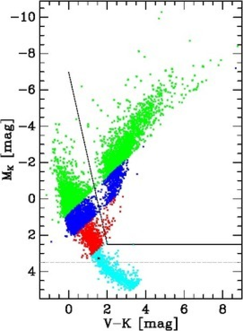
Figure 1: Colour-magnitude diagram of the Hipparcos stars used for this study. The colour coding is as follows – green: stars with $M_{V}\leq$ 0.8 mag and within 200 pc of the Sun; dark blue: stars with 0.8 $<M_{V}\leq$ 2.3 mag and within 100 pc; red: stars with 2.3 $<M_{V}\leq$ 4.3 mag and within 40 pc, and light blue: stars with 4.3 $<M_{V}\leq$ 8.3 mag and within 25 pc, respectively, see also table 1. In the construction of our LF we have used Hipparcos stars with $M_{K}\leq$ 3.5 mag (dashed line). The solid line cuts our giant sample off our dwarf stars. The black cross in the light blue dotted area denotes the Sun.

Since we derive distances and also base our absolute magnitudes on Hipparcos parallaxes the associated error (which we assume to be Gaussian) can affect our sample selection. The skewed error distribution after inverting parallaxes to distances results in the so called parallax bias (Francis, 2013) leading to larger mean distances. Another effect of the parallax error arising from the volume limit of the sample, but of opposite sign, is the Trumpler-Weaver or Lutz-Kelker bias (Trumpler & Weaver, 1953; Lutz & Kelker, 1973) which increases star counts as the error volume outside our limiting distance is larger than inside and more stars should scatter in. In the literature these biases are often corrected statistically but it was shown that the Lutz-Kelker correction depends strongly on the adopted spatial distribution of the sample (usually a homogeneous density is assumed) and the true absolute magnitude distribution (see e.g. Smith, 2003). The latter may be well defined for special stellar types like red clump giants or cepheids. In our case for the bright Hipparcos stars there is no simple way to calculate the Lutz-Kelker correction due to the wide spread in luminosities and stellar types. In order to assess the impact of these biases on our star counts we select all stars in the Hipparcos catalogue. We sample the parallax of each star 100 times randomly as a Gaussian with the mean of the original star’s observed parallax and the standard deviation of its associated error. Then we perform the same cuts as before, divide the counts by 100 and compare them to our sample. The 40 pc sample decreases by 1 per cent, the 100 pc sample increases by 2 per cent, and the 200 pc sample decreases by 2 per cent. Relaxing the parallax error cuts yield similar corrections. In effect the corrections are small and show no clear trend in star counts as well as in the luminosity function so that we can safely neglect them.

A more severe source of error is dust extinction close to the Galactic plane. Due to missing 3D maps of the highly inhomogeneous dust distribution in the solar neighbourhood we cannot correct for this error and only give rough estimates on its magnitude. For that we use the analytic extinction model from Rybizki & Just (2015) based on Vergely et al. (1998) which gives a good estimate for the mean extinction. It represents a slab of constant dust density up to a distance of 55 pc from the midplane with a hole at the solar position representing the local bubble. The resulting extinction vanishes for stars closer than 70 pc (inside the local bubble) and at Galactic latitudes $|b|>52^{o}$. The extinction reaches its maximum of about $A_{V}=0.19$ mag at the limiting distance of 200 pc in the Galactic plane. Applying the same procedure as before but now also correcting for extinction nothing changes for the 40 pc sample. For the 100 pc and 200 pc samples the star counts increase by 2.4 per cent and 6.6 per cent, respectively. Overall, neglecting extinction leads to a slightly underestimated luminosity function for bright stars with $M_{V}<2.3$ mag. This bias is stronger for dwarfs at the upper main sequence, because of their stronger concentration to the midplane. On the other hand the derived luminosity distribution and total brightness in the K band is dominated by giants, which have a larger scale height and therefore being less obscured by extinction.

The faint end of the LF has been determined using an updated version of the Fourth Catalogue of Nearby stars (hereafter CNS5, in prep.; CNS4, Jahreiß & Wielen, 1997). All CNS5 stars within 25 pc were cross matched with the 2MASS catalogue. From the 4622 CNS5 stars within 25 pc 135 stars got K-magnitudes from other sources. Only 6 close binaries were removed at all as well as 9 brown dwarfs and one white dwarf below the magnitude limit of the 2MASS survey. For the missing stars, $K$-magnitudes were obtained from the literature, from spectral types, or applying an $M_{K}$–($V-K$) relation based on CNS5 stars with accurate parallaxes and reliable colours. The resulting CNS5 sample is illustrated in Fig. 2 as a colour-magnitude diagram $M_{K}$ vs ($J-K$).

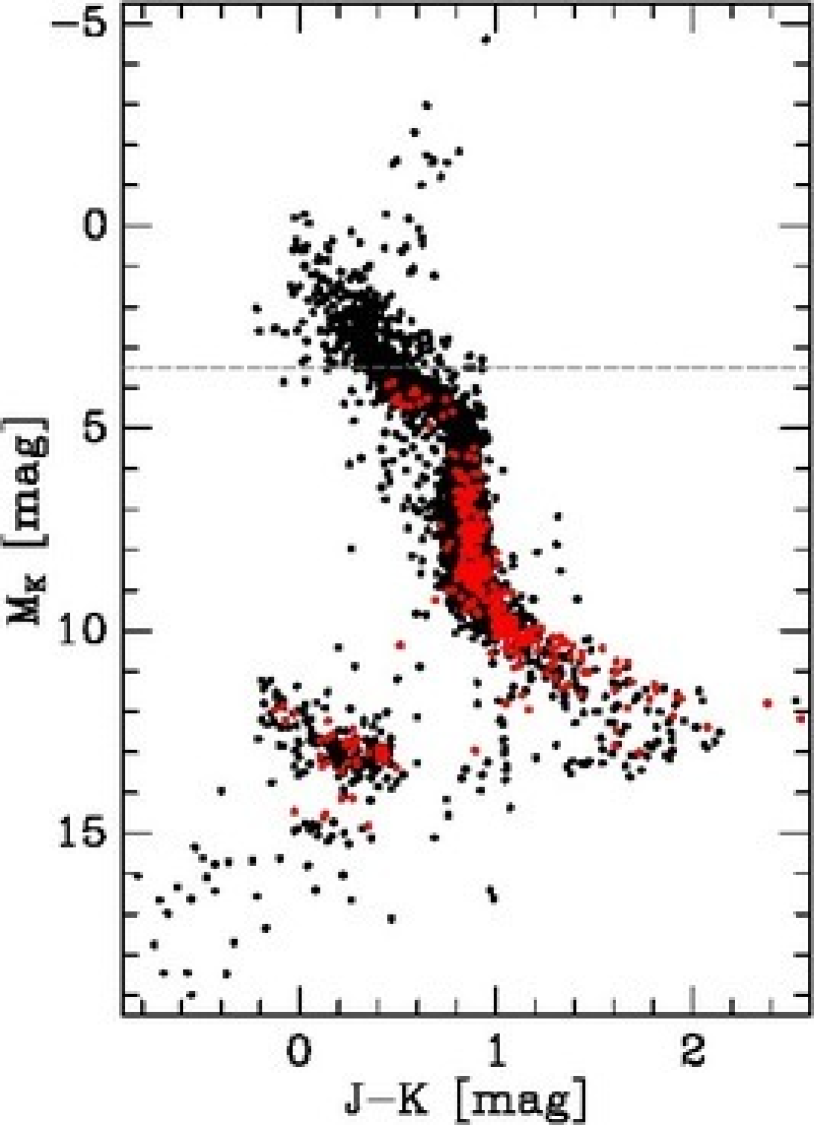
Figure 2: Colour-magnitude diagram representing our CNS5 stars. Shown here are only stars with reliable distance estimates: For 3520 stars (black) trigonometric parallaxes are available, while for the remaining 365 stars photometric distances were adopted (red symbols). In the actual construction of the LF we have used CNS5 stars fainter than $M_{K}=$ 3.5 mag (dashed line).

2.1 Completeness and vertical profiles

Our Hipparcos samples are volume complete by construction. But beyond about $\pm 40$ pc perpendicular to the Galactic plane, stellar densities decline with increasing distance from the plane, and lead to significant correction factors converting the mean luminosity density in the observed volume to the local luminosity density at the Galactic midplane. It can be easily shown that the impact of a (distance dependent) incompleteness, if present, on the cumulative number of stars $N_{\mathrm{z}}$ as function of $z$ is mainly an apparently reduced local density $n_{0}$, but the shape $N_{\mathrm{z}}/n_{0}$ is essentially unaffected. We thus use $N_{\mathrm{z}}$ to determine the vertical density profiles and correct for the local volume density at the midplane for the $r_{0}=$100 pc and the 200 pc samples, separately for both giant and dwarf stars. Within a sphere of radius $r_{0}$, a constant density is obtained if the cumulative number of stars $N_{\mathrm{z}}$ follows the relation $N_{\mathrm{z}}=2\pi n_{0}z(r_{0}^{2}-z^{2}/3)$ (grey dotted lines in Fig. 3). We tested different vertical density profiles (linear, exponential with and without a shallow core or Gaussian) and investigated the impact of an offset of the solar position $z_{\mathrm{\sun}}$ from the midplane. It turns out that the profiles of the dwarfs in both samples can be better fit with $z_{\mathrm{\sun}}=15$ pc.

For the 200 pc sample, the cumulative star counts deviate significantly from the constant density fit of the inner 80 and 50 pc for giants and dwarfs, respectively, which yields a local number density of $8.8\times 10^{-5}\mathrm{pc}^{-3}$ for the giants and 1 per cent less for the dwarfs. Instead the giants are best fit by an exponential profile with a local number density $n_{0}=9.35\times 10^{-5}\mathrm{pc}^{-3}$ and an exponential scale height of 456 pc. The dwarfs are better fit by a cored exponential profile with flat density at the midplane and local density of $n_{0}=9.90\times 10^{-5}\mathrm{pc}^{-3}$ and an exponential scale height of $z_{exp}=44$ pc at large $|z|\gg z_{exp}$. The flat profile near the midplane and the small scale height as well as the corresponding half-thickness of $h=88$ pc are expected for B and early A stars with velocity dispersions $\sigma\approx 5$ km s^-1 (see Fig. 9). The result is also consistent with the vertical density profile of the A star population derived in Holmberg & Flynn (2000). We note that the midplane densities are 5 - 10 per cent larger than the value from the linear fit at small $|z|$. The conversion factors $f_{200}=n_{0}/\langle n\rangle$ from the mean number densities $\langle n\rangle=N_{\mathrm{f}in}/V_{200}$ ($V_{200}$ is the volume of the 200 pc sphere) to the local number densities $n_{0}$ are $f_{200,g}=1.18$ and $f_{200,d}=1.85$ for giants and dwarfs, respectively.

Investigating the 100 pc sample yields an almost constant density for the giants. The best fit with an exponential density profile yields a local density $n_{0}=1.38\times 10^{-4}\mathrm{pc}^{-3}$ and an exponential scale height of 500 pc (see lower panel of Fig. 3). The dwarfs of this sample are best fit by an exponential profile with a local number density $n_{0}=4.34\times 10^{-4}\mathrm{pc}^{-3}$ and an exponential scale height of 173 pc. The corresponding conversion factors are $f_{100,g}=1.07$ and $f_{100,d}=1.23$ for giants and dwarfs, respectively.

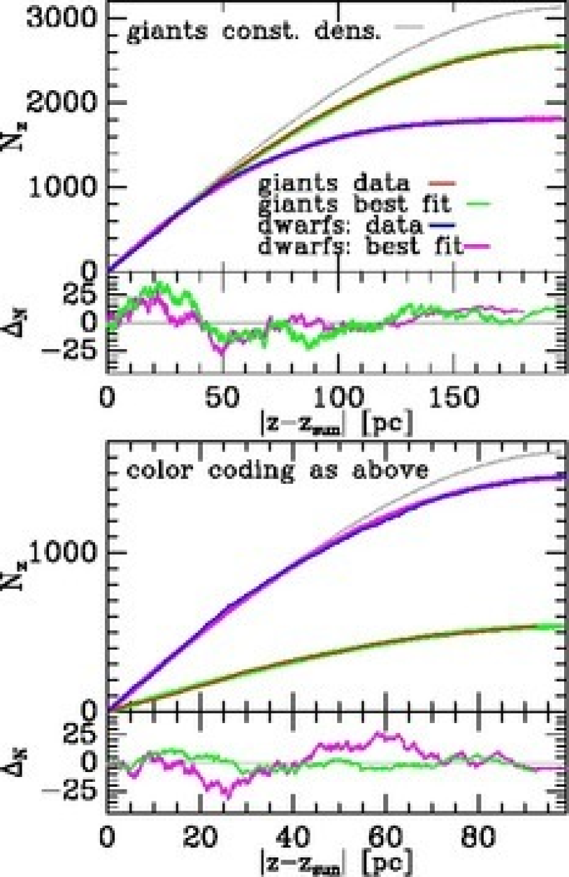
Figure 3: Top panel: Cumulative distributions $N_{z}$ in $|z-z_{\mathrm{\sun}}|$ of the 2 660 giants (red) and 1 796 dwarfs (blue) in the 200 pc-sphere. Best fits of the vertical density profiles are shown in green and pink lines, respectively. For comparison the grey dotted line shows the expectation for a constant density. The differences of model and data $\Delta_{N}$ are also shown in the inset. The slopes at small $z$ of giants and dwarfs determining the local number density differ by a few per cent only, which is by chance due to the sample selection in the 200 pc sphere. The lower panel shows the same for the 100 pc sample with 541 giants and 1477 dwarfs.

Our faint star counts are based on the CNS5 and suffer from incompleteness, which we assume to depend on distance only. We have assessed the completeness of the CNS5 by carrying out radial cumulative star counts in each magnitude bin (with a width of 1 mag). These are shown in Fig. 4. In a spatial homogeneous sample the cumulative number of stars $n$ grows with distance $d$ as $n\,\propto\,d^{3}$. In a double logarithmic log($n$) vs ($-$log($\pi$)) representation of Fig. 4 – where $\pi$ is the stellar parallax – a homogeneous sample would appear as a straight line with slope 3 (green lines).

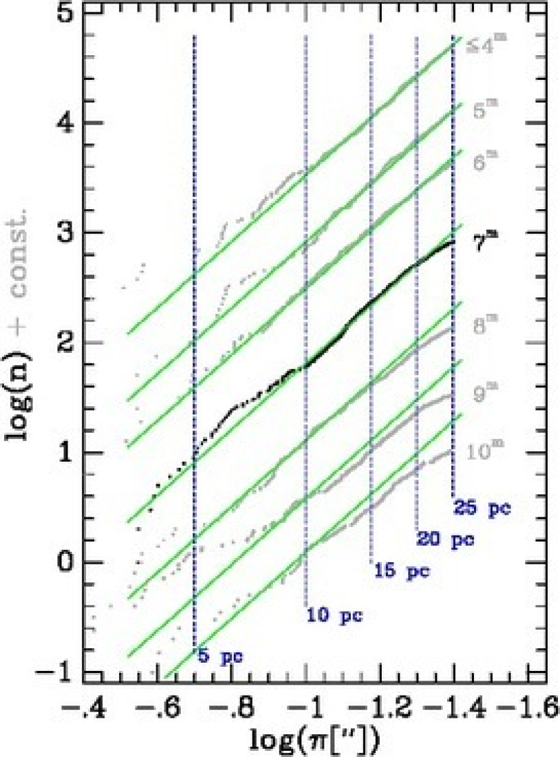
Figure 4: Radial cumulative star counts of CNS5 stars in magnitude bins (bin width 1 mag) ranging from $M_{K}=4$ mag and brighter to $M_{K}=10$ mag (grey points). For clarity log(n) has been shifted arbitrarily along the vertical axis for all but the $M_{K}=7$ mag sample which is plotted in black. The green lines indicate spatially homogeneous samples with the adopted local density.

The completeness limit of the CNS5 in each magnitude bin can be seen by a deviation of the actual star counts from the line of slope 3. From Fig. 4 we read off the completeness limits summarized in Table 2. The magnitude bins $M_{K}$ = 13 and 14 mag are dominated by white dwarfs. For magnitudes fainter than $M_{K}$ = 14 mag the completeness limit cannot be reliably determined. In order to derive a lower limit for the star number densities we have considered a volume with a radius of 10 pc. White dwarfs in the solar neighbourhood are completely sampled out to a distance of $d\sim 13$ pc from the Sun (Holberg et al., 2008). The stellar number densities given in the next section have been determined within each completeness limit and were then converted to a standard (spherical) volume with a radius of 20 pc.

The luminosity function of the CNS5 stars alone is illustrated in Fig. 5. In order to demonstrate how the volume completeness of the CNS5 influences the predictions of the LF, we have split up the original volume of the CNS5 (with a radius of 25 pc) into spherical shells of 5 pc width. The luminosity functions derived from each shell are over-plotted onto each other in Fig. 5. As can be seen here all shells give within statistical errors consistent results up to an absolute magnitude of $M_{K}$ = 5 mag. Beyond that magnitude the outer shells yield reduced star numbers, because they become increasingly incomplete.

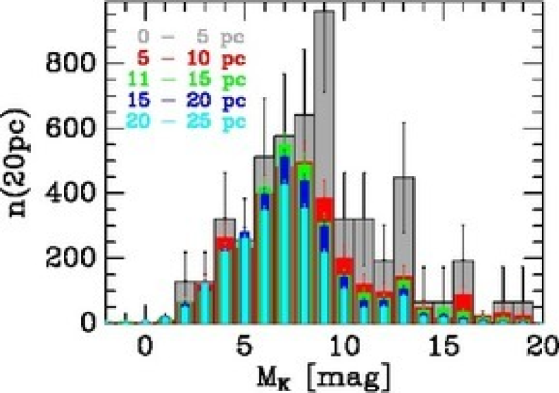
Figure 5: Illustration of the distance effect on the NIR LF. The volume of the CNS5 has been split into spherical shells of 5 pc width. The LFs derived from each shell are over–plotted in colour coding onto each other.

3 Luminosity function and its Implications

We constructed the local NIR luminosity function $\Phi(M_{K})$ in terms of star numbers in the 20 pc sphere $V_{20}=33\,510$ pc³ as described in the previous section by combining the samples of stars brighter than $M_{K}=3.5$ mag drawn from the Hipparcos catalogue and fainter stars from the CNS5. We will now discuss $\Phi(M_{K}$), the luminosity budget, and the mass functions that result.

3.1 Local luminosity function

We show the results of our determination of the local luminosity function in Table 2. Given errors indicate the (usually dominating) Poisson errors. We first note how smoothly the Hipparcos and CNS5 samples join together in the $M_{K}\,$= 2 and 3 magnitude bins, see columns 3 and 5. The Hipparcos sample is volume complete down to $M_{K}\,$= 4 mag. However, binary stars have been treated more carefully in the CNS5 than in the Hipparcos sample as evinced by slightly larger star numbers in these magnitude bins (cf. Table 2). In column 9 of Table 2 the luminosity function of the dwarfs alone (main sequence and turnoff stars) is shown. This was derived by excluding giants according to the dividing line in the CMD as discussed earlier (cf. Fig. 1) and similarly white dwarfs in the bins $M_{K}=$11–14 mag were removed.

Table 2: Stellar luminosity function $\Phi(M_{K})$.

$M_{K}$	Sp	$\Phi_{Hip}$	limits	$\Phi_{CNS}$	err	$\Phi_{comb}$	err	$\Phi_{MS}$	Mass
[mag]	[ ]	(*)	[pc]	(*)	(*)	(*)	(*)	(*)	[${\mathcal{M}}_{\odot}$]
(1)	(2)	(3)	(4)	(5)	(6)	(7)	(8)	(9)	(10)
$-$10	M3,4 I–II	0.0024				0.0024	0.0017
$-$9	K–M2 I–II	0.0012				0.0012	0.0012
$-$8	M8 III	0.0145				0.0145	0.0090
$-$7	A,G I–II, M6,7 III	0.0333				0.0333	0.0101
$-$6	M4,5 III	0.0767				0.0767	0.0095
$-$5	M1–3 III	0.186		0.5	0.9	0.186	0.015
$-$4	M0 III	0.321		0.		0.321	0.020	0.0093	19.6
$-$3	B0,1, K4,5 III	0.699		0.5	0.9	0.699	0.030	0.0389	15.0
$-$2	K2,3 III	2.611		4.1	1.5	2.611	0.098	0.0981	10.8
$-$1	B2,3,G8–K0 III	3.492		1.0	0.8	3.492	0.157	0.531	6.1
0	B5–A0, F8–G2 III	5.512		7.7	2.0	5.512	0.441	3.135	3.46
1	A2–A5	18.49		16.9	3.0	18.49	1.01	15.73	1.98
2	F5	53.95		48.1	5.0	53.95	2.57	51.94	1.47
3	F8–G2 V	112.2		119.8	7.9	112.2	6.8	111.7	1.14
4	G5–K4 V	184.3	25	220.2	10.7	220.2	10.7	220.2	0.80
5	K5–M1 V	76.80	25	261.1	11.6	261.1	11.6	261.1	0.63
6	M2–3 V		20	397.0	20.0	397.0	20.0	397.0	0.48
7	M4–5 V		20	512.0	22.7	512.0	22.7	512.0	0.27
8			10	496.0	63.0	496.0	63.0	496.0	0.16
9			10	384.0	55.5	384.0	55.5	384.0	0.11
10			10	200.0	40.0	200.0	40.0	200.0	0.07
11			10	120.0	31.0	120.0	31.0	112.0
12			10	96.0	27.8	96.0	27.8	80.0
13			10	144.0	34.0	144.0	34.0	48.0
14			10	48.0	19.6	48.0	19.6	16.0
15			10	$>$ 16.0	11.4	$>$ 16.0	11.4	$>$ 16.0
16			10	$>$ 88.0	26.6	$>$ 88.0	26.6	$>$ 88.0
17			10	$>$ 24.0	13.9	$>$ 24.0	13.9	$>$ 24.0
18			10	$>$ 32.0	16.0	$>$ 32.0	16.0	$>$ 32.0

The total LF and the contributions of dwarfs and giants are shown in the top panel of Fig. 6. Since the number of giants is very small, the giant LF is multiplied by a factor of 100 to make it visible. The dwarf LF shows a clear maximum at $M_{K}$ = 7–8 mag beyond which it drops by nearly an order of magnitude at $M_{K}$ = 13 mag. The faint end of the LF in the L, T dwarf regime is unreliable due to the large error bars and incompleteness. The shape of $log(\Phi(M_{K}))$ is roughly consistent with the LF observed in the optical bands as is illustrated in Fig. 6, bottom panel. Both the NIR and V band main-sequence LFs are shown together with the analytical fit by Mamon & Soneira (1982) to the V band LF of Wielen (1974), and its theoretical transformation into the 2.2 $\mu$m filter band. As can be seen from Fig. 6 the analytic models fit very well in the F – K dwarf regime. At the very bright end ($M_{K}\leq 1$ mag) the observed LF falls below the theoretical prediction.

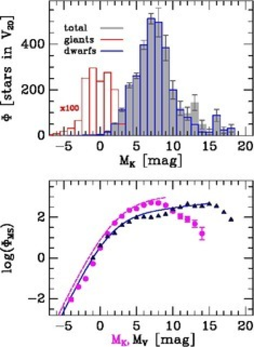
Figure 6: Top panel: Histogram of $\Phi(M_{K})$ for all stars (grey histogram), dwarf stars (blue) and giants (red). For clarity $\Phi(M_{K})$ of the giants has been enhanced by a factor of 100 in the red histogram. The contribution of white dwarfs at $M_{K}\approx 13$ mag is clearly visible. Bottom panel: Comparison of the main sequence LFs in the V band (triangles) and in the NIR (pink circles). The blue line is an analytical fit to the optical data and the pink one a theoretical transformation of it to the K band. $\Phi_{MS}$ is given as number of stars in the 20pc sphere $V_{20}$.

3.2 Local luminosity distribution

In the previous section we have given the luminosity function $\Phi(M_{K})$, i.e. the number of stars in absolute magnitude bins. In order to calculate the contribution of each bin to the total local luminosity in $V_{20}$, we now multiply $\Phi(M_{K})$ with the mean luminosity $L_{K}$ = 10${}^{-0.4({M_{K}}-{M_{K\odot})}}L{{}_{K\odot}}$ of the bin, where $M_{K\odot}$ denotes the absolute $K$-magnitude of the Sun $M_{K\odot}=3.27$ mag (Casagrande et al., 2012). The result is illustrated in Fig. 7 and again the contributions of dwarfs and giants are shown. The dwarf luminosity distribution peaks at $M_{K}=2$ mag corresponding to F type stars and is analogous to the peak at $M_{V}=1$ mag in the optical luminosity distribution (Flynn et al., 2006). The contribution of the faint end with $M_{K}>8$ mag is completely negligible. The luminosity distribution of giants does not show a clear maximum. In contrast, the contribution at the very bright end of supergiants beyond $M_{K}=-5$ mag is dominating in the NIR. Due to the low number statistics at $M_{K}<-8$ mag the contribution of the brightest end is very uncertain. Red clump giants are responsible for the large value at $M_{K}=-2$ mag. In the V band the luminosity distribution of giants strongly declines for $M_{V}<1$ mag (Flynn et al., 2006).

We find for the total K band luminosity $\rho_{K}=0.1205\pm 0.0036\,L_{K\odot}$pc^-3, now converted to the local luminosity density. The uncertainty is dominated by the bright end of the giants. The giants dominate with 0.0971 $\pm$ 0.0036 $L_{K\odot}$pc^-3 (80 per cent) and the dwarfs contribute 20 per cent with $0.0234\pm 0.0005$ $L_{K\odot}$pc^-3. A re–calculation of the V band luminosity of the same sample yields 0.053  $L_{V\odot}$pc^-3 (slightly smaller than the old value $\rho_{V}=0.056\,L_{V\odot}$pc^-3 of Flynn et al., 2006). Combining the local K- and V band luminosity results in $(V-K)=2.46$ mag in the solar neighbourhood (with $(V-K)_{\odot}=1.56$ mag). This colour is slightly bluer than the value of $(V-K)=2.55$ mag determined in model A of Just & Jahreiss (2010) based on a Scalo IMF.

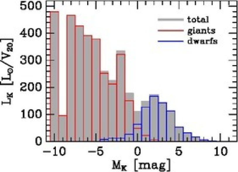
Figure 7: Local luminosity distribution in the NIR (grey histogram). The contribution by giants is shown with the red line, the blue line indicates the contribution by main sequence stars.

3.3 Local mass distribution

We next examine how the NIR luminosity function relates to the mass distribution of the stars. For this purpose we have multiplied the numbers of stars with mean masses of the stars in each $M_{K}$ magnitude bin. For dwarfs, the adopted masses are reproduced in the last column of Table 2. For absolute magnitudes 3.1 $\leq$ $M_{K}$ $\leq$ 9.8 mag we have used directly the absolute magnitude $M_{K}$-mass relation by Henry & McCarthy (1993). For main sequence stars brighter than $M_{K}=$ 3 mag we have used the $M_{V}$-mass relation compiled by Andersen (1991) which we have transformed to $M_{K}$ by applying $V-K$ main sequence colours. For red giants we assume a mass of 1.4 $\pm$ 0.1 ${\mathcal{M}}_{\odot}$ as derived by Stello et al. (2008) from asteroseismic observations. Supergiants may be significantly more massive than that (Schmidt-Kaler, 1982), but are so few that their mass densities are negligible. The resulting mass distributions for giants and main sequence stars, which we have been able to estimate without recourse to population synthesis modeling (Bell & de Jong, 2001; Zibetti, Charlot & Rix, 2009), are illustrated in Fig. 8 as a function of absolute $M_{K}$ magnitude. The small contribution of giants is scaled up by a factor of 10 for visibility. In contrast to the luminosity distribution (see Fig. 7) the local mass density is dominated by the lower main sequence with $M_{K}>2$ mag.

The local mass density of main sequence and giant stars is $0.0315$ and $0.00058\,{\mathcal{M}}_{\odot}$ pc^-3, respectively. For the total stellar mass density we need to add the contribution of brown dwarfs and white dwarfs. For brown dwarfs we add 0.002 ${\mathcal{M}}_{\odot}$ pc^-3 assuming a 50 per cent incompleteness in the observational data of late M, T and L dwarfs. For the local mass density of white dwarfs we use 0.0032 $\pm$ 0.0003 ${\mathcal{M}}_{\odot}$ pc^-3 (Holberg et al., 2008), which is similar to our finding of 0.0030 $\pm$ 0.0009 ${\mathcal{M}}_{\odot}$ pc^-3. This way, we find a total local mass density of $\rho=0.0373\,{\mathcal{M}}_{\odot}$ pc^-3 for the stellar component. The total stellar density is slightly smaller than in earlier determinations (0.039, 0.044, 0.0415 ${\mathcal{M}}_{\odot}$ pc^-3; Jahreiß & Wielen, 1997; Holmberg & Flynn, 2000; Flynn et al., 2006, respectively). In all three publications a larger contribution of white dwarfs was adopted. Additionally, in Holmberg & Flynn (2000) and Flynn et al. (2006) the mass of the upper MS ($M_{V}<2.5$ mag) was overestimated, and in Holmberg & Flynn (2000) the contribution of BDs was too high.

The local mass density implies a mass-to-light ratio of the stellar component in the local volume of $M/L_{K}\,=\,0.31\pm 0.02\,{\mathcal{M}}_{\odot}/L_{K\odot}$. This can be compared with the optical mass-to-light ratio of $0.707\,{\mathcal{M}}_{\odot}/L_{V\odot}$, which is smaller than the value of $0.75\,{\mathcal{M}}_{\odot}/L_{V\odot}$ derived in Flynn et al. (2006) mainly due to the smaller local mass density.

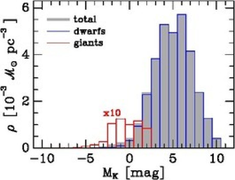
Figure 8: Distribution of the mass density $\rho$ for the stellar part of the Milky Way disc (grey histogram). Stellar mass densities are given as a function of absolute $M_{K}$ magnitudes (blue lines : main sequence stars, red lines : giants). For clarity the mass densities of the giants have been enhanced by a factor of 10 in the red histogram.

3.4 NIR Surface brightness of the local disc

The results presented so far reflect the NIR LF as well as the luminosity and mass distributions as functions of $M_{K}$ for the Milky Way in the solar neighbourhood. More representative for the entire Milky Way disc is the local surface brightness, i.e. the local luminosity distribution multiplied by the vertical scale heights of the stars. The calculations of surface brightness and surface density depend on the adopted disc model, because for most sub–populations there are no direct observations of the vertical density profile available. It was demonstrated in Flynn et al. (2006) that the vertical scale heights $h$ of the various stellar populations can be roughly estimated by their vertical velocity dispersions $\sigma$, because in a given gravitational potential the vertical scale heights are in lowest order directly proportional to the latter. For an improved estimation of the surface brightness we use a higher order fit of the (half-)thickness $h(\sigma)$ defined by $\Sigma=2\,h\,n_{0}$ connecting the local volume density $n_{0}$ and the surface density $\Sigma$ of the tracer. For a non–exponential vertical profile of the tracer the thickness $h$ differs from the exponential scale height. Each stellar subpopulation is approximated by an isothermal component in the total potential characterized by the local density $\rho_{0}=0.102{\mathcal{M}}_{\odot}$ pc^-3 and effective scale height $z_{0}=280$ pc leading to

$$h(\sigma)=\sqrt{\frac{\pi}{2}}\cdot z(\sigma)+\frac{z(\sigma)^{2}}{3\,z_{0}}\quad\mbox{with}\quad z(\sigma)=\frac{\sigma}{\sqrt{4\pi G\rho_{0}}}.$$ (1)

The dotted line in the lower panel of Fig. 9 shows the approximation for the thin disc. The parameters $\rho_{0}$ and $z_{0}$ are chosen to reproduce the values $h(\sigma)$ of the detailed local disc model of Just & Jahreiss (2010) as well as the mass model used in Holmberg & Flynn (2000); Flynn et al. (2006) (triangles in the lower panel of Fig. 9). The parameters are optimized such that the fit function can also be used for the thick disc with velocity dispersion $\sigma\approx 40$ km s^-1.

The upper panel of Fig. 9 shows the measured vertical velocity dispersions in each $M_{K}$ bin and Hipparcos group for the giants. At the bright end the velocity dispersions scatter around a constant value of 17.3 km s^-1, whereas the faint giants in the 40 pc group show a large scatter and a larger mean value of 22.7 km s^-1. Since the outliers do not contribute much to the total luminosity, we will use the same constant $\sigma_{g}=17.3$ km s^-1 for all giants. For the upper main sequence dwarfs in the Hipparcos samples we show the mean values in each $M_{K}$ bin (weighted by the number densities in the 20 pc volume in order to avoid a bias due to the increasing age with increasing $V\,-\,K$). To all lower main sequence stars we have assigned the mean velocity dispersion of G, K dwarfs – falling in the $M_{K}=5$ mag bin – from Table 4 of Jahreiß & Wielen (1997) because the CNS5 is kinematically biased to high proper motion stars at lower magnitudes and we expect – and assume here – the same kinematics for all these stars. Their $\sigma$ values are shown as open symbols in Fig. 9. In this figure the blue line shows the analytic fit, using a shifted error function, of $\sigma(M_{K})$ for the dwarfs, which we use to convert the velocity dispersions to the corresponding thickness $h$.

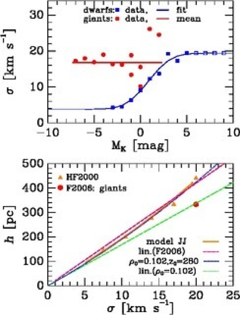
Figure 9: Conversion of velocity dispersion to thickness in 2 steps. Top: Observed vertical velocity dispersions $\sigma$ for dwarfs and giants in each magnitude bin together with the analytic approximations. For the meaning of open symbols, see text. Bottom: Vertical thickness $h$ of the analytic fit used for the transformation (blue dotted line), for the best Just-Jahreiss-model (JJ model A, solid orange line), the values for the mass model used in Holmberg & Flynn (2000) (HF2000, orange triangles) and in Flynn et al. (2006) (red dashed line and F2006 for giants, red circle). For comparison the linear extrapolation based on the total local density is also shown (green dashed line).

Additionally a correction for the thick disc contribution is necessary. Adopting a standard isothermal old thick disc with a velocity dispersion of 40 km s^-1 corresponds to a thickness $h=1031$ pc. In the solar neighbourhood we assume a thick disc fraction of 10 per cent for all giants and for the lower main sequence with $M_{K}>1.5$ mag. Due to the larger thickness this fraction is enhanced accordingly for the surface brightness. The surface brightness of each subpopulation $i$ is given by $\Sigma_{K,i}=2\,h_{i}\,L_{K,i}$.

The resulting surface brightness distribution is shown in Fig. 10, where we find similar features as in the local luminosity distribution (Fig. 7). The distribution is strongly dominated by the bright end of the giants, the red clump giants are visible in the $M_{K}$ =  -2 mag bin, and the dwarfs peak at the F dwarfs. The integrated surface brightness is $\Sigma_{K}=98.7\,L_{K\odot}$pc${}^{-2}=19.9$ mag arcsec^-2 in total, composed by $16.2\,L_{K\odot}$pc^-2 (16 per cent) for dwarfs and $82.5\,L_{K\odot}$pc^-2 (84 per cent) for giants. Antares alone has added 5.3 $L_{K\odot}$pc^-2 demonstrating the uncertainty due to Poisson noise for the brightest supergiants.

A similar determination of the V band surface brightness distribution shows a similar shape, but with a less dominant red giant contribution (cf. discussion above). We find $29.1\,L_{V\odot}$pc${}^{-2}=22.7$ mag arcsec^-2. This value is 19 per cent larger than the value of $24.4\,L_{V\odot}$pc^-2 determined by Flynn et al. (2006) arising from inconsistencies in the earlier transformation to surface brightness as can be seen by comparing their Figures 2, 5 and 6. In the I band, which Flynn et al. (2006) have used to derive the location of the Milky Way with respect to the Tully-Fisher (TF) relation, their Figures 9 and 10 seem to be correct. Combining the K and V band surface brightnesses yields $(V-K)=2.89\,$mag for the solar cylinder.

The corresponding stellar mass surface density derived from the local mass distribution (Fig. 8) including white dwarfs and brown dwarfs is 33.3 ${\mathcal{M}}_{\odot}$ pc^-2, which is slightly smaller than the value 35.5 ${\mathcal{M}}_{\odot}$ pc^-2 of Holmberg & Flynn (2004); Flynn et al. (2006). It implies a K band mass-to-light ratio of $M/L_{K}\,=\,0.34\,{\mathcal{M}}_{\odot}/L_{K\odot}$. The corresponding optical mass-to-light ratio is $M/L_{V}\,=\,1.14\,{\mathcal{M}}_{\odot}/L_{V\odot}$.

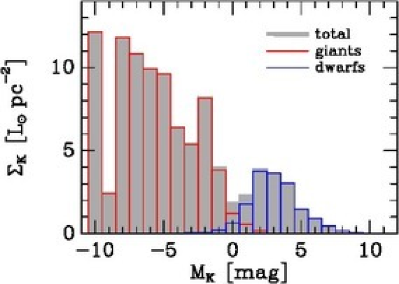
Figure 10: Surface brightness distribution in the NIR. The blue and red lines indicate the contributions by the main sequence stars and giants, respectively.

3.5 Tully-Fisher relation

The surface brightness of the disc in the solar cylinder can be used to estimate the total K band luminosity of the Milky Way and compare it with the observed Tully-Fisher (TF) relation of extragalactic systems. We proceed similar as in Flynn et al. (2006) for the I band. The total disc luminosity is approximately independent of the adopted radial scalelength $h_{R}$ in the range of 2.5–5 kpc. For definiteness we adopt $h_{R}=3.5$ kpc and find with $\Sigma_{K}=98.7\,L_{K\odot}$pc^-2 at the solar radius of $R_{0}=8$ kpc a total disc luminosity of $8.0\times 10^{10}\,L_{K\odot}$. Adding the bulge luminosity of $1.5\times 10^{10}\,L_{K\odot}$ (Drimmel & Spergel, 2001; Portail et al., 2015) yields a total luminosity of $M_{K}=-24.2$ mag. In Fig. 11 the data point adopting a maximum rotation velocity of the Milky Way disc of $220\pm 20$ km s^-1 and an estimated uncertainty in the total luminosity of 0.2 mag is shown. For comparison we plotted two determinations of the TF relation in the K band based on 2MASS data. Karachentsev et al. (2002) used edge-on galaxies to derive the isophotal TF relation in K band using $K_{20}=20$ mag arcsec^-2. We have adapted their TF relation from Fig. 8 to a Hubble constant of $H_{0}=70$ km s^-1 Mpc^-1. For the Milky Way seen edge-on $K_{20}$ is at $R\approx 20$ kpc including more than 98 per cent of the total light. The Milky Way is 0.2 mag brighter than the TF relation. For an alternative TF relation we show in Fig. 11 also the corrected equations of Masters et al. (2008, 2014) applied to an Sbc type galaxy. In this case the Milky Way is 0.2 mag fainter than the TF relation. The systematic differences of the two TFs arise mainly on the inclination dependence of the $K_{20}$ isophotal luminosity (see also Said et al., 2015) and the uncertainties in the extrapolation to the total luminosity. Deeper K band observations may solve this issue in the future. For the Milky Way seen face-on the isophotal luminosity would be 0.4 mag fainter than seen edge-on.

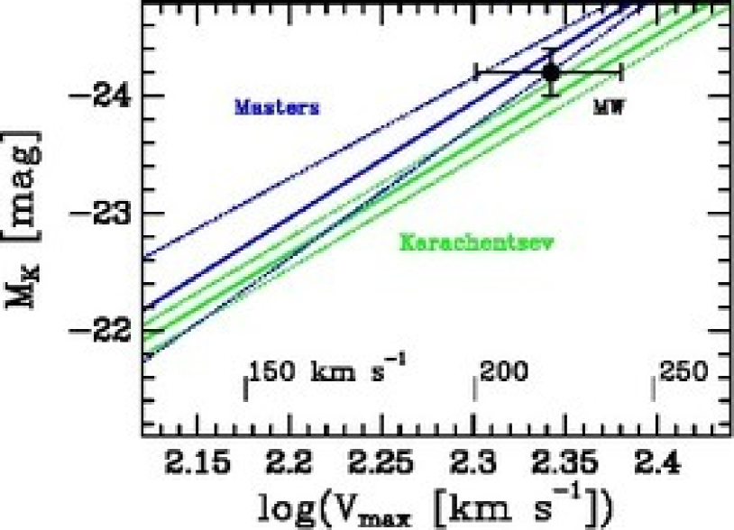
Figure 11: The Milky Way (dot with uncertainty bars, MW) with respect to the TF relations of Karachentsev et al. (2002); Masters et al. (2014), respectively. Dotted lines show the 1-sigma scatter in the TFs.

4 Conclusions

We have constructed a new sample of stars representative for the solar neighbourhood. The data set is based on two subsets separated by the intrinsic brightness of the stars. The bright part comprises stars drawn from the survey part of the Hipparcos catalogue. The faint part $M_{K}>3.5$ mag is based on the CNS5, an updated version of the Fourth Catalogue of Nearby Stars. Each star has been identified in the 2MASS catalogue so that we have individually determined NIR photometry in a homogeneous system for all stars (typically $K_{\rm s}$) available.

For the Hipparcos stars we have selected volume complete samples in $M_{V}$ magnitude bins and corrected for the vertical density profile to determine the midplane density. These subsamples were then resampled in $M_{K}$ magnitude bins for $M_{K}\leq 3.5$ mag. The spatial completeness of the CNS5 sample has been carefully examined by cumulative radial star counts for each $M_{K}$ bin resulting in a reasonable estimate of the local number density as faint as the $M_{K}=14$ mag bin, which is well in the brown dwarf regime. For fainter stars we derived lower limits for the corresponding star numbers per magnitude bin. All star numbers have been converted to a fiducial spherical volume with a radius of 20 pc (centered on the Sun) and constant density as a measure of the local volume density. For a detailed analysis we have separated the giants and white dwarfs from main sequence stars including turnoff stars and brown dwarfs. We have then determined the NIR luminosity function of the stars in the Milky Way disc by direct star counts in our sample. The K band luminosity function shows a strong maximum at $M_{K}=7-8$ mag. At $M_{K}=13-14$ mag the white dwarfs dominate the star counts.

The luminosity function has then been converted to the luminosity distribution of the stars by multiplying the star numbers with the typical luminosities of the stars in each absolute magnitude bin. The resulting (midplane) luminosity distribution is strongly dominated by the very bright end of giants and supergiants. A secondary peak at $M_{K}$ $\approx$ 2 mag is due to A – F type main sequence stars while at $M_{K}=-2$ mag the red clump giants stick out. At the bright end there is no decline measurable, which means that the low number statistics of the brightest supergiants dominate the uncertainty of the total local luminosity in the K band. We find a total luminosity density of $\rho_{K}=0.121\pm 0.004\,L_{K\odot}$pc^-3, where the giants dominate with a contribution of 80 per cent. Combined with the V band luminosity density of $\rho_{V}=0.053\,L_{V\odot}$pc^-3 we find a value of $V-K=2.46$ mag for the colour in the solar neighbourhood.

We have determined the mass distribution of the stars as probed by the NIR luminosity function in the same way. Quite contrary to the NIR light, the mass of the Milky Way is dominated by K and M main sequence stars. We conclude from this discussion that the mass–carrying population of stars in galactic discs cannot be observed directly in the NIR on a star-by-star basis. The total mass density of the stellar component is $\rho=0.0373\,M_{\odot}$pc^-3, which is about 10 percent smaller than earlier determinations due to reduced contributions by white dwarfs and brown dwarfs. The local mass-to-light ratio is then $M/L_{K}\,=\,0.31\,{\mathcal{M}}_{\odot}/L_{K\odot}$. The corresponding corrected value in the optical is $M/L_{V}\,=\,0.71\,{\mathcal{M}}_{\odot}/L_{V\odot}$.

For a comparison to extragalactic systems it is important to determine the surface brightness of the disc. We have used a detailed vertical disc model to derive the effective thickness of the stellar populations in the magnitude bins and took into account a correction for the thick disc contribution with a larger thickness. The resulting surface brightness function shows similar features as the local luminosity distribution. The total surface brightness is $99\,L_{K\odot}$pc${}^{-2}=5.4\times 10^{-6}$ W m^-2 with 84 per cent resulting from giants. This value can be compared to the $K$ band surface brightness of the disc determined from DIRBE data after removing all point sources yielding $68\,L_{K\odot}$pc^-2 (Melchior, Combes & Gould, 2007). The difference corresponds to the contribution of all supergiants with $M_{K}<-8$ mag, which seems reasonable. The mass model yields a surface density of $33.3\,M_{\odot}$pc^-2 and a mass-to-light ratio for the solar cylinder of $M/L_{K}\,=\,0.34\,{\mathcal{M}}_{\odot}/L_{K\odot}$. The corresponding optical surface brightness and mass-to-light ratio is $29.1\,L_{V\odot}$pc^-2 and $M/L_{V}\,=\,1.14\,{\mathcal{M}}_{\odot}/L_{V\odot}$, respectively. With the redetermination of the surface brightness we have corrected a bug in the earlier determination by Flynn et al. (2006), which happened particularly in the V band. An extrapolation of the local surface brightness to the whole Milky Way yields a total K band luminosity of $M_{K}=-24.2$ mag. With standard values of the disc properties the Milky Way falls between the Karachentsev et al. (2002) and Masters et al. (2014) K band TF relations.

The stellar population in the solar neighbourhood is strongly dominated by young stars compared to the population in the solar cylinder due to the much smaller scale heights of the young populations. Nevertheless, the mass-to-light ratio in the K band is only 10 per cent larger in the solar cylinder. The reason for the luminosity of the present day giants – dominating the light in the K band – being a rough measure of stellar mass, carried by F, G, and K stars of the lower main sequence, is the similarity of their age distributions. The birth time distribution for the precursors of the giants – mainly F and G dwarfs – is spread over the age of the disc and similar to that of the F, G, and K dwarfs still on the main sequence. As a consequence, the dynamical evolution is similar and produces comparable scale heights. Thus we conclude that the mass-to-light ratio does not vary strongly in disc populations with a long star formation history and a calibration of the absolute value is provided by the solar neighbourhood properties.

The colours and mass-to-light ratios are consistent with the stellar populations derived in the local disc model of Just & Jahreiss (2010). Into & Portinari (2013) determined mass-to-light ratios and colours for disc populations with exponentially declining star formation histories. Our values are roughly consistent with these models for relatively flat star formation histories. An extrapolation from the solar radius to the whole disc would shift the colour and mass-to-light ratios slightly dependent on the disc growth model. Our K band mass-to-light ratio of the solar cylinder of $0.34\,{\mathcal{M}}_{\odot}/L_{K\odot}$ is very close to the mean value of $0.31\,{\mathcal{M}}_{\odot}/L_{K\odot}$ of 30 disc galaxies derived by Martinsson et al. (2013).

References

- Andersen (1991) Andersen J., 1991, A&ARv, 3, 91
- Bell & de Jong (2001) Bell E. F., de Jong R. S., 2001, ApJ, 550, 212
- Casagrande et al. (2012) Casagrande L., Ramirez I., Melendez J., Asplund M., 2012, ApJ, 761, 16
- Drimmel & Spergel (2001) Drimmel R., Spergel D. N., 2001, ApJ, 556, 181
- Flynn et al. (2006) Flynn C., Holmberg J., Portinari L., Fuchs B., Jahreiß H., 2006, MNRAS, 372, 1149
- Francis (2013) Francis C., 2013, MNRAS, 436, 1343
- Garwood & Jones (1987) Garwood R., Jones T. J., 1987, PASP, 99, 453
- Gliese (1969) Gliese W., 1969, Veröff. ARI, Nr. 22, Braun, Karlsruhe
- Henry & McCarthy (1993) Henry T. J., Mc Carthy D. W., 1993, AJ, 106, 773
- Holberg et al. (2008) Holberg J. B., Sion E. M., Oswalt T., McCook G. P., Foran S., Subasavage J. P., 2008, AJ, 135, 1225
- Holmberg & Flynn (2000) Holmberg J., Flynn C., 2000, MNRAS, 313, 209
- Holmberg & Flynn (2004) Holmberg J., Flynn C., 2004, MNRAS, 352, 440
- Houk & Fesen (1978) Houk N., Fesen R., 1978, IAUS, 80, 91
- Into & Portinari (2013) Into T., Portinari L., 2013, MNRAS 430, 2715
- Jahreiß & Wielen (1997) Jahreiß H., Wielen R., 1997, in Battrick B., Perryman M. A. C., Bernacca P. L., eds., Hipparcos-Venice 97, ESA SP-402, 675
- Just & Jahreiss (2010) Just A., Jahreiß H., 2010, MNRAS, 402, 461
- Karachentsev et al. (2002) Karachentsev I. D., Mitronova S. N., Karachentseva V. E., Kudrya Y. N., Jarrett T. H., 2002, A&A 396, 431
- Koorneef (1983) Koorneef J., 1983, A&A, 128, 84
- van Leeuwen (2007) van Leeuwen F., 2007, A&A, 474, 653
- López-Corredoira et al. (2002) López-Corredoira, M., Cabrera-Lavers A., Garzón F., Hammersley P. L., 2002, A&A, 394, 883
- Lutz & Kelker (1973) Lutz T. E., Kelker D. H., 1973, PASP, 85, 573
- Martinsson et al. (2013) Martinsson T. P. K., Verheijen M. A. W., Westfall K. B., Bershady M. A., Andersen D. R., Swaters R. A., 2013, A&A, 557, A131
- Mamon & Soneira (1982) Mamon G. A., Soneira R. M., 1982, ApJ, 255, 181
- Masters et al. (2008) Masters K. L., Springob C. M., Huchra J. P., 2008, AJ 135, 1738
- Masters et al. (2014) Masters K. L., Springob C. M., Huchra J. P., 2014, ApJ, 147, 124 (erratum to Masters et al., 2008)
- McGaugh & Schomberg (2014) McGaugh S. S., Schombert J. M., 2014, arXiv:1407.1839
- Melchior, Combes & Gould (2007) Melchior A.-L., Combes F., Gould A., 2007, A&A, 462, 965
- Perryman et al. (1997) Perryman M. A. C. et al., 1997, The Hipparcos and Tycho Catalogues, ESA SP-1200
- Picaud, Cabrera-Lavers & Garzón (2003) Picaud S., Cabrera-Lavers A., Garzón F., 2003, A&A, 408, 141
- Portail et al. (2015) Portail M., Wegg C., Gerhard O., Martinez-Valpuesta, I., 2015, MNRAS, 448, 713
- Ruelas-Mayorga (1991) Ruelas-Mayorga R. A., 1991, Rev. Mex. Astron. Astrofis., 22, 43
- Rhoads (1998) Rhoads J. E., 1998, AJ, 115, 472
- Rix & Rieke (1993) Rix H.-W., Rieke M. J., 1993, ApJ, 418, 123
- Rybizki & Just (2015) Rybizki J., Just A., 2015, MNRAS, 447, 3880
- Said et al. (2015) Said K., Kraan-Korteweg R. C., Jarrett T. H., 2015, MNRAS, 447, 1618
- Schmidt-Kaler (1982) Schmidt-Kaler Th., 1982, Landolt-Börnstein, Group 6, Vol. 2, p. 21
- Skrutskie, Cutri & Stiening (2006) Skrutskie M. F., Cutri R. M., Stiening R., 2006, AJ, 131, 1163
- Smith (2003) Smith H. Jr, 2003, MNRAS, 338, 891
- Stello et al. (2008) Stello D., Bruntt H., Preston H., Buzasi D., 2008, ApJ, 674, L53
- Trumpler & Weaver (1953) Trumpler R. J., Weaver H. F., 1953, Statistical Astronomy. Dover Books on Astronomy and Space Topics, Dover Publications, New York
- Vergely et al. (1998) Vergely J.-L., Ferrero R. F., Egret D., Koeppen J., 1998, A&A, 340, 543
- Wainscoat et al. (1992) Wainscoat R. J., Cohen M., Volk K., Walker H. J., Schwartz D. E., 1992, ApJS, 83, 111
- Wielen (1974) Wielen R., 1974, in Highlights of Astronomy, Vol. 3; G. Contopoulos (ed.), Reidel, Dordrecht, p. 395
- Zibetti, Charlot & Rix (2009) Zibetti S., Charlot S., Rix H.-W., 2009, MNRAS, 400, 1181