Identification of Matrices having a Sparse Representation

We consider the problem of recovering a matrix from its action on a known vector in the setting where the matrix can be represented efficiently in a known matrix dictionary. Connections with sparse signal recovery allows for the use of efficient reconstruction techniques such as Basis Pursuit. Of particular interest is the dictionary of time-frequency shift matrices and its role for channel estimation and identification in communications engineering. We present recovery results for Basis Pursuit with the time-frequency shift dictionary and various dictionaries of random matrices.

1 Introduction

Inferring reliable information from limited data is a key task in the sciences. For example, identifying a channel operator from its response to a limited number of test signals is a crucial step in radar and communications engineering [25, 32, 34, 40, 43, 49]. Here we consider the canonical setting where an operator is approximated by a linear map, that is, by a matrix $\bm{\Gamma}\in{\mathbb{C}}^{n\times m}$. While it is clear that $\bm{\Gamma}$ is determined by its action on any $m$ vectors that span ${\mathbb{C}}^{m}$, significantly fewer measurements may be sufficient if a-priori information about the operator is at hand. For instance, one commonly considers the question whether a single test signal $\bm{h}$, referred to also as identifier, can be used to identify $\bm{\Gamma}$ from $\bm{\Gamma}\bm{h}$. A priori information guaranteeing that such an $\bm{h}$ exists is generally deduced from physical considerations which may ensure that $\bm{\Gamma}$ can be efficiently represented or approximated using relatively few basic matrices from a known matrix dictionary.

In wireless communications ([13, 28, 41] and references within) and sonar [39, 50], for example, the narrowband regime of a transmission channel can generally be well approximated by a linear combination of a small number of time-frequency shift matrices. Signals travel from the source to the receiver along a number of different paths, each of which can be modeled by a time shift (delay dependent on the length of the path traveled) and a frequency shift (Doppler effect caused by the motion of the transmitter, of the receiver, and of reflecting objects) [5, 28]. It is frequently assumed, that the number of relevant (but unknown) paths, that is, in slightly simplified terms the number of involved time-frequency shifts is relatively small when compared to the symbol length. For example, for mobile communications the number of paths required to well approximate a channel in rural areas or typical urban regiments does not exceed 10 [41, pages 266,283], see also [10, 13]. In wireless communications the benefit of recovering the operator at the receiver is clear. Knowledge of the operator is necessary to invert it and to recover the information carrying channel input from the channel output.

Complexity regularization has recently seen a resurgence of interest in the signal processing community under the monikers sparse signal recovery and sparse approximation. In sparse signal recovery, one seeks the solution of an underdetermined system of equations $\bm{Ax}=\bm{b}$, $\bm{A}\in{\mathbb{C}}^{n\times N}$, $n<N$, with $\bm{x}$ having the fewest number of non-zero entries from all solutions of $\bm{Ax}=\bm{b}$. We show in Section 2 that the identification of a matrix from its action on a single test signal falls into the same setting as sparse signal recovery when the matrix is known to have a sparse representation. This observation allows us to adopt efficient algorithms from sparse signal recovery for the sparse matrix identification question. Examples of applications include the channel identification, estimation, or sounding problem described in part above, which also have been considered in the case of time-invariant channels in [11, 14, 30]. Numerical results based on Basis Pursuit have been obtained for time-varying channels in [48]. Further, the application of recovery methods of sparsely represented operators to radar measurements is discussed in [32].

In brief, the content of this paper is organized as follows. In Section 2 we formalize the matrix identification problem for matrices with sparse representations. We establish a connection to the recovery problem of vectors with sparse representations and state the main results that are proven and discussed in greater detail in Section 4 and Section 5. In particular, we consider matrix ensembles of random Gaussian or Bernoulli matrices as well as partial Fourier matrices (Section 2.1 and Section 4).

In Section 2.2 and Section 5 we consider matrix dictionaries of time-frequency shift matrices which are of particular interest due to their efficacy in approximating time-varying transmission channels. We would like to emphasize that the common framework of the identification problem for matrices with a sparse representation and the sparse signal recovery problem implies that the results achieved on the recovery of matrices with a sparse representation in the dictionary of time-frequency shift matrices are at the same time results for the recovery of signals with a sparse representation in Gabor frames.

In Section 6 we briefly discuss the use of several test vectors instead of just one, and comment on how this improves corresponding recovery results.

We conclude with numerical experiments in Section 7. They verify our main results concerning sparse representations with time-frequency shift matrices stated in Theorem 2.5, and show that the precise recoverability thresholds follow those proven for Gaussian random matrices in [24]; that is, for matrices having a $k$-sparse representation we observe Basis Pursuit to successfully recover the matrix from its action on a single vector provided $k\leq n/(2\log n)$.

2 Main results and context

Before comparing the matrix identification problem with sparse signal recovery, we formalize the notion of a matrix having a $k$-sparse representation.

Definition 2.1

A matrix $\bm{\Gamma}$ has a $k$-sparse representation in the matrix dictionary $\bm{\Psi}=\{\bm{\Psi}_{j}\}_{j=1}^{N}$ if

$$\bm{\Gamma}=\sum_{j}x_{j}\bm{\Psi}_{j}\quad\quad\mbox{with}\quad\|\bm{x}\|_{0}=k,$$

and $\|\bm{x}\|_{0}$ counts the number of non-zero entries in $\bm{x}$, that is $\|\bm{x}\|_{0}=|{\rm supp}\,\bm{x}|={\rm cardinality}\{x_{j}:\,x_{j}\neq 0\}$.

The set of elementary matrices comprising $\bm{\Psi}$ may form a basis for ${\mathbb{C}}^{n\times m}$ but it may as well only span a subspace of ${\mathbb{C}}^{n\times m}$ and/or contain linearly dependent subsets. In Definition 2.1 we place no restrictions on the dictionary $\bm{\Psi}$.

Identification of matrices having a sparse representation from their action on a single vector (henceforth referred to simply as sparse matrix identification, which is not to be confused with the notion of sparse matrices in numerical analysis) can be formulated as sparse signal recovery problem through the simple observation that the action of $\bm{\Gamma}$ on a test signal $\bm{h}\in{\mathbb{C}}^{m}$ can be expressed as

$$\bm{\Gamma}\bm{h} {=} \Big{(}\sum_{j=1}^{N}x_{j}\bm{\Psi}_{j}\Big{)}\bm{h}=\sum_{j=1}^{N}x_{j}\big{(}\bm{\Psi}_{j}\bm{h}\big{)}=\left(\bm{\Psi}_{1}\bm{h}\,|\,\bm{\Psi}_{2}\bm{h}\,|\,\ldots\,|\,\bm{\Psi}_{N}\bm{h}\right)\bm{x}{=}(\bm{\Psi}\bm{h})\bm{x}$$ (1)

where $\bm{x}=(x_{1},\;x_{2},\;\cdots,\;x_{N})^{T}$ and $(\bm{\Psi}\bm{h})=(\bm{\Psi}_{1}\bm{h}\,|\,\bm{\Psi}_{2}\bm{h}\,|\,\ldots\,|\,\bm{\Psi}_{N}\bm{h}).$

In classical sparse signal recovery the sparsest vector $\bm{x}$ satisfying $\bm{Ax}=\bm{b}$ is sought given $\bm{b}$ and $\bm{A}$; to identify the matrix $\bm{\Gamma}$, $\bm{\Gamma}\bm{h}$ takes the place of $\bm{b}$ and the $j^{th}$ column of $\bm{A}$ is $\bm{\Psi}_{j}\bm{h}$ for $j=1,2,\ldots,N$.

As mentioned above, we note that in case of the $\bm{\Psi}_{j}$ being time-frequency shift matrices, the columns in $\bm{A}=(\bm{\Psi}\bm{h})$ form a Gabor system with window $\bm{h}$ [12, 29, 37]. Consequently, all our identifiability results concerning representations with time-frequency shift matrices are also results for the recovery of signals that are sparse in a Gabor system.

Remark 2.2

Although sparse matrix identification can be cast as sparse signal recovery, two important differences should be noted.

• In most applications, sparse signal recovery is only of interest for $k$-sparse vectors with $k<n$, as the linear dependence of the $N$ columns of $\bm{A}\in{\mathbb{C}}^{n\times N}$, $n<N$, implies that $n$-term solutions $\bm{x}$ for $\bm{Ax}=\bm{b}$ are never unique. However, in some cases an $n$-term solution might be of interest if there is no sparser solution of $\bm{Ax}=\bm{b}$. In contrast, the goal in sparse matrix identification is not to represent $\bm{b}=\bm{\Gamma}\bm{h}$ efficiently, but to recover $\bm{\Gamma}$. The non-uniqueness of $n$-term solutions to $(\bm{\Psi}\bm{h})\bm{x}=\bm{\Gamma}\bm{h}$ implies that there always exist infinitely many $n-$sparse matrices $\bm{\Gamma}^{\prime}$ consistent with the observations $\bm{\Gamma}^{\prime}\bm{h}=\bm{\Gamma}\bm{h}$. As such, the recovery of an $n$-sparse $\bm{x}$ in the sparse matrix identification setting does not give any information about the matrix to be identified, $\bm{\Gamma}$.

• In sparse signal recovery the columns of $\bm{A}$ are used to represent or to approximate $\bm{b}$, whereas for sparse matrix identification the matrices $\bm{\Psi}_{j}$ are used to represent or approximate $\bm{\Gamma}$. However, unlike sparse signal recovery where the columns of $\bm{A}$ appear explicitly in the reconstruction, the $\bm{\Psi}_{j}$ do not appear explicitly when sparse matrix identification is cast as sparse signal recovery (1); rather, only the action of $\bm{\Psi}_{j}$ on the test vector $\bm{h}$ is utilized. The test vector $\bm{h}\in{\mathbb{C}}^{m}$ has no analog in traditional sparse signal recovery, and can be exploited in sparse matrix identification to design desirable characteristics in $\bm{\Psi}_{j}\bm{h}$. This design freedom is utilized extensively in our main results concerning the matrix dictionary of time-frequency shifts, Theorem 2.5.

Note that the computational difficulty in sparse signal recovery, sparse approximation, and our formulation of sparse matrix identification arises from the fact that the support set of the non-zero entries in $\bm{x}$ is unknown. While the direct solution of finding the sparsest representation of $\bm{\Gamma}$ in the dictionary $\bm{\Psi}$

$$\min\|\bm{x}^{\prime}\|_{0}\quad\mbox{subject to}\quad(\bm{\Psi}\bm{h})\bm{x}^{\prime}=\bm{\Gamma}\bm{h},$$ (2)

involves a combinatorial search of the support set and is therefore computationally intractable, a number of computationally efficient algorithms have been shown to recover the sparsest solution if appropriate conditions are met. We concentrate here on recoverability conditions for the canonical sparse signal recovery algorithm Basis Pursuit (BP) where the convex problem

$$\min\|\bm{x}^{\prime}\|_{1}\quad\mbox{subject to}\quad(\bm{\Psi}\bm{h})\bm{x}^{\prime}=\bm{\Gamma}\bm{h},$$ (3)

$\|\bm{x}\|_{1}=\sum_{j}|x_{j}|$, is solved as a proxy to (2).

The convex program (3) can be solved efficiently using well established optimization algorithms for second-order cone programming and linear programming [6, 18, 33], for complex and real valued systems, respectively. We give theoretical and numerical evidence for conditions where the solution of (3) coincides exactly with that of (2). Many other algorithms may also be used as proxys for (2), including Orthogonal Matching Pursuit (OMP) [26, 36, 52], stagewise orthogonal matching pursuit (StOMP) [16], and an algorithm based upon error correcting codes [2]–to name a few. Our principal technical results in Section 5.1 also give results for OMP, but for conciseness we do not state them here, leaving them to the interested reader.

In practice, the measured vector $\bm{\Gamma}\bm{h}$ will be contaminated by noise, and, in addition, the operator $\bm{\Gamma}$ will not be strictly sparse, but will instead be well approximated by a sparse representation; in this case the minimization problem (3) will be replaced by its well known variant

$$\min\|\bm{x}^{\prime}\|_{1}\quad\mbox{subject to}\quad\|(\bm{\Psi}\bm{h})\bm{x}^{\prime}-\bm{\Gamma}\bm{h}\|_{2}\leq\epsilon,$$ (4)

where $\|\bm{z}\|_{2}=\sqrt{\sum_{j}|z_{j}|^{2}}$ as usual.

2.1 Dictionaries of random matrices

Many known results in sparse signal recovery, sparse approximations and their companion theory of compressed sensing involve random matrices [4, 9, 15, 24, 46]. Based on these results, we obtain recovery results for matrix dictionaries where all its member matrices are chosen at random. From a practical point of view such random matrix dictionaries do not seem to be useful in the sparse matrix identification setting; nevertheless, the statements give some insight into the sparse matrix identification question as they give guidance in what kind of results to seek in the mathematical analysis of structured and more application relevant matrix dictionaries.

Theorem 2.3

Let $\bm{h}$ be a non-zero vector in ${\mathbb{\mathbb{R}}}^{m}$.

• Let all entries of the $N$ matrices $\bm{\Psi}_{j}\in{\mathbb{\mathbb{R}}}^{n\times m}$, $j=1,\ldots,N$ be chosen independently according to a standard normal distribution (Gaussian ensemble); or

• let all entries of the $N$ matrices $\bm{\Psi}_{j}\in{\mathbb{\mathbb{R}}}^{n\times m}$, $j=1,\ldots,N$ be independent Bernoulli $\pm 1$ variables (Bernoulli ensemble).

Then there exists a positive constant $c$ so that for $\varepsilon>0$,

$$k\leq c\,\frac{n}{\log\big{(}\frac{N}{n\varepsilon}\big{)}}$$

implies that with probability of at least $1-\varepsilon$ all matrices $\bm{\Gamma}$ having a $k$-sparse representation with respect to $\bm{\Psi}=\{\bm{\Psi}_{j}\}$ can be recovered from $\bm{\Gamma}\bm{h}$ by Basis Pursuit (3).

Using Theorem 3.6, this recovery result can be made stable under perturbation of $\bm{\Gamma}\bm{h}$ by noise, and also applies when $\bm{\Gamma}$ is not exactly $k$-sparse, but can be well approximated by a $k$-sparse operator.

Precise information on the constant $c$ will be given in Section 4. In case of the Gaussian ensemble Donoho and Tanner [17, 19, 20, 23, 24] obtained sharp thresholds separating regions in the ($k/n$, $n/N$) plane where recovery holds or fails with high probability; Section 4.1 recounts these and additional results on Gaussian systems. Theorem 2.3(b) is proven in Section 4.2, and similar results for certain diagonal matrices are proven in Section 4.3.

2.2 The dictionary of time-frequency shift matrices

As outlined in the introduction, the matrix dictionary of time-frequency shifts appears naturally in the channel identification problem in wireless communications [5] or sonar [50]. Due to physical considerations wireless channels may indeed be modeled by sparse linear combinations of time-frequency shifts $\bm{M}_{\ell}\bm{T}_{p}$, where the periodic translation operators $\bm{T}_{p}$ and modulation operator $\bm{M}_{\ell}$ on ${\mathbb{C}}^{n}$ are given by

$$(\bm{T}_{p}\bm{h})_{q}=h_{(p+q)\!\!\!\!\!\mod{n}},\;\;(\bm{M}_{\ell}\bm{h})_{q}=e^{2\pi i\ell q/n}h_{q}.$$ (5)

The system of time-frequency shifts,

$$\bm{\mathcal{G}}=\{\bm{M}_{\ell}\bm{T}_{p}:\ell,p=0,\ldots,n{-}1\},$$ (6)

forms a basis of ${\mathbb{C}}^{n\times n}$ and for any non-zero $\bm{h}$, the vector dictionary $\bm{\mathcal{G}}\bm{h}$ is a Gabor system [29, 35, 37]. Below, we focus on the so-called Alltop window $\bm{h}^{A}$ [3, 51] with entries

$$h^{A}_{q}\,=\,\frac{1}{\sqrt{n}}e^{2\pi iq^{3}/n},\quad q=0,\ldots,n{-}1,$$ (7)

and the randomly generated window $\bm{h}^{R}$ with entries

$$h^{R}_{q}\,=\,\frac{1}{\sqrt{n}}\epsilon_{q},\quad q=0,\ldots,n{-}1,$$ (8)

where the $\epsilon_{q}$ are independent and uniformly distributed on the torus $\{z\in{\mathbb{C}},|z|=1\}$.

Invoking existing recovery results [22, 27, 52, 53] (see Theorems 3.1 and 3.2 below) and our results on the coherence of Gabor systems $\bm{\mathcal{G}}\bm{h}^{A}$ and $\bm{\mathcal{G}}\bm{h}^{R}$ in Section 5.1, see Section 2.4, we will obtain

Theorem 2.4

• Let $n$ be prime and $\bm{h}^{A}$ be the Alltop window defined in (7). If $k<\frac{\sqrt{n}+1}{2}$ then Basis Pursuit recovers from $\bm{\Gamma}\bm{h}^{A}$ all matrices $\bm{\Gamma}\in{\mathbb{C}}^{n\times n}$ having a $k$-sparse representation, $\bm{\Gamma}=\sum_{(p,\ell)\in\Lambda}x_{p\ell}\bm{M}_{\ell}\bm{T}_{p}$, $|\Lambda|=k$, with respect to the time-frequency shift dictionary $\bm{\mathcal{G}}$ given in (6).

• Let $n$ be even and choose $\bm{h}^{R}$ to be the random unimodular window in (8). Let $t>0$ and suppose

  $$k\leq\frac{1}{4}\sqrt{\frac{n}{2\log n+\log 4+t}}+\frac{1}{2}\,.$$ (9)

  Then with probability of at least $1-e^{-t}$ Basis Pursuit recovers from $\bm{\Gamma}\bm{h}^{R}$ all matrices $\bm{\Gamma}\in{\mathbb{C}}^{n\times n}$ having a $k$-sparse representation with respect to the time-frequency shift dictionary $\bm{\mathcal{G}}$ given in (6).

A slight variation of part (b) also holds for $n$ odd, but is omitted for conciseness. Further note that Theorem 2.4 also holds with Basis Pursuit literally being replaced by Orthogonal Matching Pursuit [52]. Moreover, Theorem 3.2 shows that recovery is stable under perturbation of $\bm{\Gamma}\bm{h}^{A}$ and $\bm{\Gamma}\bm{h}^{R}$ by noise.

In contrast with Theorem 2.3 for random matrices, where $k$ is allowed to be of order ${\cal O}(n/\log n)$, Theorem 2.4 requires $k$ to be of order $\sqrt{n}$ or $\sqrt{n/\log n}$. Substantially larger order thresholds, ${\cal O}(n/\log n)$ for $\bm{h}^{A}$ and ${\cal O}(n/\log^{2}(n))$ for $\bm{h}^{R}$, are also possible to identify a matrix $\bm{\Gamma}$ which is the linear combination of a small number of time-frequency shift matrices. However, this larger regime of successful recovery necessitates passing from a worst case analysis for sparse $\bm{\Gamma}$ to an average case analysis in the sense that the coefficient vector $\bm{x}$ is chosen at random. Theorem 2.5 will follow from recent work by Tropp, [54], and our coherence results in Section 5.1, see Section 5.3.

Theorem 2.5

Let $k\geq 3$ and let $\Lambda$ be chosen uniformly at random among all subsets of $\{0,\ldots,n{-}1\}^{2}$ of cardinality $k$. Suppose further that $\bm{x}\in\mathbb{C}^{n}$ has support $\Lambda$ with random phases $({\rm sgn}(x_{\ell p}))_{(\ell,p)\in\Lambda}$ that are independent and uniformly distributed on the torus $\{z,|z|=1\}$. Let

$$\bm{\Gamma}=\sum_{(\ell,p)\in\Lambda}x_{\ell p}\bm{M}_{\ell}\bm{T}_{p}.$$

• Let $n$ be prime and choose the Alltop window $\bm{h}^{A}$ from (7). Assume that for $\epsilon>0$

  $$k\leq\frac{n}{8\log(2n^{2}/\epsilon)}$$ (10)

  and

  $$s := \frac{1}{144}\left(e^{-1/4}/2-\frac{2k}{n}\right)^{2}\frac{n}{k\log(k/2+1)}\geq 1$$ (11)

  Then with probability at least

  $$1-(\epsilon+(k/2)^{-s})$$

  Basis Pursuit (3) recovers $\bm{\Gamma}$ from $\bm{\Gamma}\bm{h}^{A}$.

• Let $n$ be an even number and choose the random window $\bm{h}^{R}$ from (8). Assume

  $$k\leq\frac{n}{32(\sigma+2)\log(n)\log(2n^{2}/\epsilon)}$$

  for some $\sigma>0$ and

  $$s := \frac{1}{576(\sigma+2)}\left(e^{-1/4}/2-\frac{2k}{n}\right)^{2}\cdot\ \frac{n}{k\log(k/2+1)}\geq 1$$

  Then with probability at least

  $$1-(\epsilon+4n^{-\sigma}+(k/2)^{-s})$$

  Basis Pursuit (3) recovers $\bm{\Gamma}$ from $\bm{\Gamma}\bm{h}^{R}$. (A similar result also holds for $n$ odd.)

In simple terms, Theorem 2.5 states that $\bm{\Gamma}$ can be recovered from $\bm{\Gamma}\bm{h}^{A}$ or $\bm{\Gamma}\bm{h}^{R}$ with high probability $1-\varepsilon$ provided that the sparsity of $\bm{\Gamma}$ satisfies $k\leq C_{\varepsilon}n/\log n$ in case of $\bm{h}^{A}$ and $k\leq C^{\prime}_{\varepsilon}n/\log(n)^{2}$ in case of $\bm{h}^{R}$.

In Section 5.4 we use a simple argument from time-frequency analysis to obtain

Corollary 2.6

Theorems 2.4, 2.5, and 5.1, also hold with the windows $\bm{h}^{A}$ and $\bm{h}^{R}$ replaced by their Fourier transforms $\widehat{\bm{h}^{A}}$ and $\widehat{\bm{h}^{R}}$, with entries defined as $\widehat{h}_{j}\,=\,\frac{1}{\sqrt{n}}\sum_{j=0}^{n{-}1}h_{q}e^{2\pi ijq/n}$.

3 Tools in sparse signal recovery

It was shown in (1) that for any test signal $\bm{h}$, we have $\bm{\Gamma}\bm{h}=(\bm{\Psi}\bm{h})\bm{x}$ where $\bm{x}$ is the sparse coefficient vector of $\bm{\Gamma}$. This observation links the sparse matrix identification question with sparse signal recovery where one seeks the sparsest solution (2) to the underdetermined system $\bm{Ax}=\bm{b}$; in the sparse matrix identification setting $(\bm{\Psi}\bm{h})\,=\,(\bm{\Psi}_{1}\bm{h}\,|\,\bm{\Psi}_{1}\bm{h}\,|\,\ldots\,|\,\bm{\Psi}_{N}\bm{h})$ takes the place of $\bm{A}$ and $\bm{\Gamma}\bm{h}$ the place of $\bm{b}$. In contrast to sparse approximation, where the dictionary $\bm{A}$ is usually fixed, for sparse matrix identification we have the additional freedom of designing the test signal $\bm{h}$ in order for $(\bm{\Psi}\bm{h})$ to have desirable properties.

Let us shortly recall known results in sparse signal recovery and sparse approximation that we apply to the sparse matrix identification question. In Section 3.1 we review the notion of coherence (12) and its implications for sparse signal recovery and approximation using Basis Pursuit, (3) and (4), as well as Orthogonal Matching Pursuit. In Section 3.2 we review the restricted isometry property, allowing for improved recoverability results for Basis Pursuit.

3.1 Coherence

The recoverability properties of sparse signal recovery algorithms for an underdetermined system $\bm{Ax}=\bm{b}$ is often measured by the coherence of $\bm{A}$,

$$\mu\,=\,\max_{r\neq s}|\langle\bm{a}_{r},\bm{a}_{s}\rangle|,$$ (12)

where $\bm{a}_{r}$ is the $r^{th}$ column of $\bm{A}$ and $\|\bm{a}_{r}\|_{2}=1$ for all $r$.

Theorem 3.1 (Tropp [52]; Donoho, Elad [21])

Let $\bm{A}$ be a unit norm dictionary with coherence $\mu$. If

$$(2k-1)\mu<1$$

then Basis Pursuit (as well as Orthogonal Matching Pursuit) recovers all $k$-sparse vectors $\bm{x}$ from $\bm{b}=\bm{Ax}$.

Recovery is also stable under perturbation by noise when Basis Pursuit (3) is replaced with (4).

Theorem 3.2 (Donoho et al. [22], Theorem 3.1)

Let $\bm{A}$, $\mu$ be as above and suppose that $(4k-1)\mu<1$. Assume that $\bm{x}$ is $k$-sparse and we have perturbed observations $\bm{b}=\bm{Ax}+\bm{z}$ with $\|\bm{z}\|_{2}\leq\epsilon$. Then the solution $\bm{x}^{\#}$ of the Basis Pursuit variant

$$\min\|\bm{x}^{\prime}\|_{1}\quad\mbox{\rm subject to}\quad\|\bm{Ax}^{\prime}-\bm{b}\|_{2}\leq\delta$$

satisfies

$$\|\bm{x}^{\#}-\bm{x}\|_{2}^{2}\leq\frac{(\epsilon+\delta)^{2}}{1-\mu(4k-1)}.$$

Theorems 3.1 and 3.2 ensure that the solutions of (3) and (4) correspond (exactly and approximately, respectively) to the solution of (2) for all $k$-sparse $\bm{x}$. For a broad class of dictionaries the coherence is of order ${\cal O}(1/\sqrt{n})$, see Sections 4 and 5 for random and Gabor dictionaries, respectively. Hence, Theorems 3.1 and 3.2 ensure (stable) recovery provided $k={\cal O}(\sqrt{n})$.

In contrast to these ${\cal O}(\sqrt{n})$ thresholds, which are valid for all $\bm{x}$, Tropp [54] developed a general framework for the analysis of Basis Pursuit (3), which is still based on the coherence of a general dictionary, but shows that (3) is often successful for substantially larger $k$ than those considered in Theorems 3.1 and 3.2. This comes, however, at the cost of assuming a random model on the sparse signal to be recovered. It allows us to prove order ${\cal O}(n/\log n)$ for $\bm{h}^{A}$ and ${\cal O}(n/\log(n)^{2})$ for $\bm{h}^{R}$ recoverability result for the time-frequency-shift dictionary, Theorem 2.5. We state the results of Tropp, where $\|\,\cdot\,\|_{2,2}$ denotes the operator norm given by $\|\bm{A}\|_{2,2}=\sup_{\|\bm{x}\|_{2}=1}\|\bm{Ax}\|_{2}$, and $\bm{A}_{\Lambda}$ is the restriction of a matrix $\bm{A}$ to the columns indexed by $\Lambda$.

Theorem 3.3 (Tropp [54], Theorem 12)

Let $\bm{A}$ be an $n\times N$ vector dictionary with unit norm columns and coherence $\mu$. Suppose that $\Lambda$ is selected uniformly at random among all subsets of $\{1,\ldots,N\}$ of size $k\geq 3$. Let $s\geq 1$. Then

$$\sqrt{144s\mu^{2}k\log(k/2+1)}+\frac{2k}{N}\|\bm{A}\|_{2,2}^{2}\leq e^{-1/4}\delta$$ (13)

implies

$${\mathbb{P}}\left(\|\bm{A}_{\Lambda}^{*}\bm{A}_{\Lambda}-\bm{Id}\|_{2,2}\geq\delta\right)\leq(k/2)^{-s}.$$

Theorem 3.4 (Tropp [54], Theorem 13)

Let $\bm{A}$ be an $n\times N$ dictionary with coherence $\mu$. Suppose $\Lambda\subseteq\{1,\ldots,N\}$ of cardinality $k$ ($|\Lambda|=k$) is such that

$$\|\bm{A}_{\Lambda}^{*}\bm{A}_{\Lambda}-\bm{Id}\|_{2,2}\leq 1/2.$$

Suppose that $\bm{x}\in\mathbb{C}^{N}$ has support $\Lambda$ with random phases ${\rm sgn}(x_{r})$, $r\in T$, that are independent and uniformly distributed on the torus $\{z,|z|=1\}$. Then with probability at least $1-2Ne^{-1/(8\mu^{2}k)}$ the sparse vector $\bm{x}$ can be recovered from $\bm{b}=\bm{Ax}$ by Basis Pursuit.

3.2 Restricted isometry property

Candès, Romberg and Tao introduced the Restricted Isometry Property (RIP) which is an alternative perspective to coherence [8, 9].

Definition 3.5

Let $\bm{A}\in{\mathbb{C}}^{n\times N}$ and $k<n$. The restricted isometry constant $\delta_{k}=\delta_{k}(\bm{A})$ is the smallest number such that

$$(1-\delta_{k})\|\bm{x}\|_{2}^{2}\leq\|\bm{Ax}\|_{2}^{2}\leq(1+\delta_{k})\|\bm{x}\|_{2}^{2}$$

for all $k$-sparse $\bm{x}$.

$\bm{A}$ is said to satisfy the restricted isometry property if it has small isometry constants, say $\delta_{k}<1/2$; such matrices allow stable sparse recovery by Basis Pursuit.

Theorem 3.6 (Candès, Romberg and Tao [8])

Assume that the restricted isometry constants of $\bm{A}$ satisfy

$$\delta_{3k}+3\delta_{4k}<2.$$

Let $\bm{x}\in\mathbb{C}^{N}$ and assume we have noisy data $\bm{y}=\bm{Ax}+\bm{\eta}$ with $\|\bm{\eta}\|_{2}\leq\epsilon$. Denote by $\bm{x}^{k}$ the truncated vector corresponding to the $k$ largest absolute values of $\bm{x}$. Then the solution $\bm{x}^{\#}$ of (4) satisfies

$$\|\bm{x}^{\#}-\bm{x}\|_{2}\,\leq\,C_{1}\epsilon+C_{2}\frac{\|\bm{x}-\bm{x}^{k}\|_{1}}{\sqrt{k}}.$$

The constants $C_{1}$ and $C_{2}$ depend only on $\delta_{3k}$ and $\delta_{4k}$.

Note that for $\bm{x}$ $k$-sparse and noise level $\epsilon=0$, Theorem 3.6 guarantees exact recovery of $\bm{x}$ by (3).

4 Random matrices

Many of the recent results in sparse signal recovery with recoverability thresholds for $k\leq Cn/\log n$ either assume that $\bm{A}$ is a random Gaussian or Bernoulli matrix [4, 9, 15, 46], or partial random Fourier matrix [7, 36, 45, 44, 47]. Recoverability results in these cases can be obtained by establishing the restricted isometry property, see Definition 3.5, or through a careful analysis of the geometric structure of the convex hull associated with the columns of $\bm{A}$ [17, 19, 20, 23, 24]. We apply these results to the matrix identification problem when the matrix has a sparse representation in terms of certain random matrices.

4.1 Gaussian matrix ensemble

Assume all entries of the $N$ matrices $\bm{\Psi}_{j}\in\mathbb{R}^{n\times m}$ in $\bm{\Psi}$ are independent standard Gaussian random variables and $\bm{h}$ is an arbitrary non-zero vector in $\mathbb{R}^{m}$. Then the entries of the dictionary $\bm{A}=(\bm{\Psi}\bm{h})\in\mathbb{R}^{n\times N}$ whose columns are given by $\bm{\Psi}_{j}\bm{h}$, $j=1,\ldots,N$, are jointly independent and of the form $Z=\sum_{\ell=1}^{n}g_{\ell}h_{\ell}$ where the $g_{\ell}$ are independent standard Gaussian random variables. By rotational invariance of the distribution of the Gaussian vector $(g_{1},\ldots,g_{n})$ the random variable $Z$ has the same distribution as $\|\bm{h}\|_{2}g$ where $g$ is a (scalar-valued) standard Gaussian. Hence, the dictionary $(\bm{\Psi}\bm{h})$ has the same distribution as $\|\bm{h}\|_{2}\bm{A}\in\mathbb{R}^{n\times N},$ where $\bm{A}$ is a random matrix whose entries are independent standard Gaussians. Thus, the existing literature in sparse approximation concerning Gaussian matrices applies, see for instance [4, 9, 15, 24, 46] and additional results discussed in the remainder of this section.

In particular, the restricted isometry property ensures stable recovery with probability at least $1-\varepsilon$ provided [4, 9, 46]

$$k\leq c\frac{n}{\log(\frac{N}{n\varepsilon})}.$$ (14)

Hence, by Theorem 3.6 we have stable recovery by (4) in this regime and the statement of Theorem 2.3(a) follows.

The work of Donoho and Tanner [19, 20] actually allows for a stronger statement than (14) in the context of noise-free and exact $k$-sparse vectors $\bm{x}$. A simple version of their results says that most $k$-sparse $\bm{\Gamma}$ can be recovered with high probability by Basis Pursuit provided $k\leq\frac{n}{2\log(N/n)}$. For details we refer to [19, 20], and for extension to the noisy setting to Wainwright’s work [55].

4.2 Bernoulli matrix ensemble

The recoverability results for Bernoulli matrices in Theorem 2.3(b) are based on establishing the restricted isometry property given in Definition 3.5.

To this end, we assume that the entries of the $N$ matrices $\bm{\Psi}_{j}\in\mathbb{R}^{n\times m}$ in $\bm{\Psi}$ are selected as independent $\pm 1$ Bernoulli variables, that is, $+1$ or $-1$ with equal probability, and let $\bm{h}$ be an arbitrary non-zero vector. Then an entry of the dictionary $\bm{A}=(\bm{\Psi}\bm{h})$ is given by

$$a_{pq}=\sum_{\ell=1}^{n}\epsilon_{\ell}^{pq}h_{\ell},\quad p=1,\ldots,m,~{}q=1,\ldots,N,$$ (15)

where the $\epsilon_{\ell}^{pq}$ are independent Bernoulli variables, that is, the $a_{pq}$ are independent Rademacher series [38]. Theorem 4.1 shows that the matrix $\bm{A}$ has the restricted isometry property with high probability for sparsities $k$ that are nearly linear in $m$. Hence, by Theorem 3.6, for an arbitrary non-zero choice of $\bm{h}$ we can recover any $\bm{\Gamma}$ having a $k$-sparse representation in terms of random Bernoulli matrices from the action of $\bm{\Gamma}\bm{h}$ through Basis Pursuit (3).

Theorem 4.1

Let $\bm{h}\in\mathbb{R}^{m}$ be normalized by $\|\bm{h}\|_{2}=1/\sqrt{m}$. Let $\bm{A}$ be the random matrix with entries defined in (15). Assume $\delta\in(0,1)$ and $t>0$. If

$$n\geq C_{1}\delta^{-2}(k\log(N/k)+\log(2e+24e/\delta)+t).$$ (16)

Then with probability at least $1-e^{-t}$ the restricted isometry property is satisfied, that is, for all $\Lambda\subset\{1,\ldots,N\}$ of cardinality at most $k$ it holds that

$$(1-\delta)\|\bm{x}\|_{2}^{2}\leq\|\bm{Ax}\|_{2}^{2}\leq(1+\delta)\|\bm{x}\|_{2}^{2}$$

for all $\bm{x}$ supported on $\Lambda$. The constant satisfies $C_{1}\leq 23.15$.

Proof. Let $\bm{v}\in\mathbb{R}^{N}$ be an arbitrary vector. We form the inner product of a row of $\bm{A}$ with $\bm{v}$,

$$X_{p}\,=\,\sum_{q=1}^{n}a_{pq}v_{q}\,=\,\sum_{q=1}^{N}\sum_{\ell=1}^{n}\epsilon_{\ell}^{pq}h_{\ell}v_{q}.$$

By independence of the $\epsilon_{\ell}^{pq}$, the $X_{p}$ are similarly independent. By Khintchine’s inequality the even moments of $X$ can be estimated by the moments of a standard Gaussian variable $g$ [38, 42]

$${\mathbb{E}}[|X_{p}|^{2z}] \leq \|\bm{v}\|_{2}\|\bm{h}\|_{2}\frac{(2z)!}{2^{z}z!}=\|\bm{v}\|_{2}\|\bm{h}\|_{2}{\mathbb{E}}[|g|^{2z}],\quad z\in\mathbb{N}.$$

Following Lemma 5 and the proof of Lemma 6 in [1] this implies the concentration inequality,

$${\mathbb{P}}(|\|\bm{Av}\|_{2}^{2}-\|\bm{v}\|_{2}^{2}|\geq\epsilon\|\bm{v}\|_{2}^{2})\leq 2\exp\left(-\tfrac{n}{2}(\epsilon^{2}/2-\epsilon^{3}/3)\right).$$

By Theorem 2.2 in [46], see also Theorem 5.2 in [4], this implies that the restricted isometry property holds under the stated condition on $n$. The estimate of the constant $C_{1}$ follows from [46, Theorem 2.2] as well. $\square$

Note that for fixed $\delta$ and $t$ condition (16) can be rewritten as

$$k\leq cn/\log(N/k)$$

for some constant $c$.

Combining Theorems 3.6 and 4.1 yields Theorem 2.3(b).

4.3 Diagonal matrices

Diagonal matrices act as multiplication operators on $\mathbb{C}^{n}$. Using a Fourier expansion of the diagonal, we observe that any diagonal matrix can be expressed as linear combination of modulation operators $\bm{M}_{\ell}\in\mathbb{C}^{n\times n}$, $\ell=0,\ldots,n{-}1$, defined in (5). We now consider the case that only a small number of components of the output of a diagonal operator $\bm{\Gamma}$ can be measured; the assumption that $\bm{\Gamma}$ is sparse in the dictionary of modulation operators shall be used to recover $\bm{\Gamma}$ from these components.

To this end, let $\Omega$ be a subset of $\{0,\ldots,n{-}1\}$ of cardinality $m$ and denote by $\bm{M}_{\ell}^{\Omega}\in\mathbb{C}^{m\times m}$ the submatrix of $\bm{M}_{\ell}$ with columns and rows restricted to the index set $\Omega$. Let

$$\bm{\Psi}^{\Omega}=\{\bm{M}^{\Omega}_{\ell},\ell=0,\ldots,n{-}1\}$$

and $\bm{h}={\mathbf{1}}=(1,\ldots,1)^{T}$. If $\bm{\Gamma}^{\Omega}=\sum_{\ell=0}^{n{-}1}x_{\ell}\bm{M}_{\ell}^{\Omega}$ then $\bm{\Gamma}^{\Omega}{\mathbf{1}}$ coincides with the restriction of $\bm{\Gamma}{\mathbf{1}}=\sum_{\ell=0}^{n{-}1}x_{\ell}\bm{M}_{\ell}{\mathbf{1}}$ to the indices in $\Omega$.

The matrix $\bm{A}$ whose columns are the elements of the dictionary $(\bm{\Psi}^{\Omega}{\mathbf{1}})=\{\bm{M}_{\ell}^{\Omega}{\mathbf{1}},\ell=0,\ldots,n{-}1\}$ is precisely a row submatrix of the Fourier matrix,

$$\bm{A}\,=\,\bm{A}^{\Omega}\,=\,(e^{2\pi ir\ell})_{r\in\Omega,\ell=0,\ldots,n{-}1}\in\mathbb{C}^{m\times n}.$$

If the subset $\Omega$ is chosen uniformly at random among all subsets of size $m$ then $\bm{A}^{\Omega}$ is a random matrix. This random partial Fourier matrix was studied in [7, 9, 47], see also [45] for a slight variation. Indeed, under the condition

$$k\leq c\,\frac{m}{\log^{4}(n)\log(\varepsilon^{-1})}$$

the restricted isometry property holds with probability at least $1-\varepsilon$ [47] and by Theorem 3.6 we obtain stable recovery of all matrices having a sparse representation in terms of $\bm{\Psi}^{\Omega}$.

5 Time-frequency shift dictionaries

In this section we establish coherence results for the dictionary of time-frequency shift matrices and prove Theorems 2.4 and 2.5.

5.1 Coherence for the time-frequency shift dictionary

We apply known recovery results [22, 27, 52, 53, 54] for dictionaries with small coherence (12). Assuming $\|\bm{h}\|_{2}=1$, the coherence, (12), of Gabor systems is

$$\mu\,=\,\max_{(\ell,p)\neq(\ell^{\prime},p^{\prime})}|\langle\bm{M}_{\ell}\bm{T}_{p}h,\bm{M}_{\ell^{\prime}}\bm{T}_{p^{\prime}}\bm{h}\rangle|.$$ (17)

Based on results by Alltop in [3], Strohmer and Heath showed in [51] that the coherence (17) of $\bm{\mathcal{G}}\bm{h}^{A}$ given in (7) satisfies

$$\mu\,=\,\frac{1}{\sqrt{n}}$$ (18)

for $n$ prime. This is almost optimal since the general lower bound in [51] for the coherence of frames with $n^{2}$ elements in $\mathbb{C}^{n}$ yields $\mu\geq\frac{1}{\sqrt{n+1}}$.

Unfortunately, the coherence (17) of $\bm{h}^{A}$ applies only for $n$ prime. For arbitrary $n$ we consider the random window $\bm{h}^{R}$.

Theorem 5.1

Let $n\in\mathbb{N}$ and choose a random window $\bm{h}^{R}$ with entries

$$h^{R}_{q}\,=\,\frac{1}{\sqrt{n}}\epsilon_{q},\quad q=0,\ldots,n{-}1,$$

where the $\epsilon_{q}$ are independent and uniformly distributed on the torus $\{z\in{\mathbb{C}},|z|=1\}$. Let $\mu$ be the coherence of the associated Gabor dictionary (17), then for $\alpha>0$ and $n$ even,

$${\mathbb{P}}\big{(}\mu\geq\frac{\alpha}{\sqrt{n}}\big{)}\leq 4n(n{-}1)e^{-\alpha^{2}/4},$$

while for $n$ odd,

$${\mathbb{P}}\big{(}\mu\geq\frac{\alpha}{\sqrt{n}}\big{)}\leq 2n(n{-}1)\left(e^{-\frac{n{-}1}{n}\alpha^{2}/4}+e^{-\frac{n+1}{n}\alpha^{2}/4}\right).$$ (19)

Up to the constant factor $\alpha$, the coherence in Theorem 5.1 comes close to the lower bound $\mu\geq\frac{1}{\sqrt{n+1}}$ with high probability. Theorems 2.4 and 2.5 will follow from these order ${\cal O}(1/\sqrt{n})$ coherence results in this section and the Theorems 3.1 and 3.2 of [22, 27, 52, 53] and Theorems 3.3 and 3.4 of Tropp [54] respectively.

Proof of Theorem 5.1. The technical details for $n$ even and odd are slightly different, for conciseness we only state the proof for $n$ even, and outline the proof for $n$ odd.

A direct computation shows that

$$|\langle\bm{M}_{\ell^{\prime}}\bm{T}_{p^{\prime}}\bm{h}^{R},\bm{M}_{\ell}\bm{T}_{p}\bm{h}^{R}\rangle|=|\langle\bm{M}_{\ell-\ell^{\prime}}\bm{T}_{p-p^{\prime}}\bm{h}^{R},\bm{h}^{R}\rangle|$$

and, therefore, it suffices to consider $\langle\bm{M}_{\ell}\bm{T}_{p}\bm{h}^{R},\bm{h}^{R}\rangle$, $\ell,p=0,\ldots,n{-}1$; furthermore, as $\langle\bm{M}_{\ell}\bm{h}^{R},\bm{h}^{R}\rangle=\langle\bm{M}_{\ell}{\mathbf{1}},|\bm{h}^{R}|^{2}\rangle=0$ for $\ell\neq 0$, we consider only the case $p\neq 0$.

Writing $\epsilon_{q}=e^{2\pi iy_{q}}$ with $y_{q}\in[0,1)$ we obtain

$$\langle\bm{M}_{\ell}\bm{T}_{p}\bm{h}^{R},\bm{h}^{R}\rangle = \frac{1}{n}\sum_{q=0}^{n{-}1}e^{2\pi i\frac{q\ell}{n}}\epsilon_{q-p}\overline{\epsilon_{q}}=\frac{1}{n}\sum_{q=0}^{n{-}1}e^{2\pi i\left(y_{q-p}-y_{q}+\frac{q\ell}{n}\right)},$$

where $\epsilon_{q-p}=\epsilon_{n+q-p}$ if $q-p<0$, that is, the indices are understood modulo $n$. Set

$$\delta_{q}^{(p,\ell)}\,=\,e^{2\pi i\left(y_{q-p}-y_{q}+\frac{q\ell}{n}\right)},$$

and note that $\delta_{q}^{(p,\ell)}$ is uniformly distributed on the torus $\mathbb{T}$. However, the $\delta_{q}^{(p,\ell)}$, $q=1,\ldots,n$, are no longer jointly independent. But nevertheless, as we demonstrate in the following, we can split all variables into two subsets of independent variables.

If $p=1$, $p=n{-}1$, or if neither $p$ nor $n-p$ divide $n$, then the $n/2$ random variables $\epsilon_{0}\overline{\epsilon_{p}},\epsilon_{p}\overline{\epsilon_{2p}},\ldots,\epsilon_{p(n/2-1)}\overline{\epsilon_{pn/2}}$ are jointly independent, as well as the remaining $n/2$ variables $\epsilon_{pn/2}\overline{\epsilon_{p(n/2+1)}},\ldots,\epsilon_{p(n{-}1)}\overline{\epsilon_{0}}$. The indices are again understood modulo $n$. If $p\geq 2$ or $n-p\geq 2$ divides $n$, then we form the $p$ random vectors

$$\bm{Y}_{1}= (\epsilon_{0}\overline{\epsilon_{p}},\epsilon_{p}\overline{\epsilon_{2p}},\ldots,\epsilon_{n-p}\overline{\epsilon_{0}}),$$

$$\bm{Y}_{2}= (\epsilon_{1}\overline{\epsilon_{p+1}},\epsilon_{p+1}\overline{\epsilon_{2p+1}},\ldots,\epsilon_{n-p+1}\overline{\epsilon_{1}}),$$

$$\vdots$$

$$\bm{Y}_{p}= (\epsilon_{p-1}\overline{\epsilon_{2p-1}},\epsilon_{2p-1}\overline{\epsilon_{3p-1}},\ldots,\epsilon_{n{-}1}\overline{\epsilon_{p-1}}).$$

These vectors are jointly independent. Moreover, $p\leq n/2$ allows partitioning the entries of a single vector $\bm{Y}$ into two sets $\Lambda_{p}^{1}$ and $\Lambda_{p}^{2}$ with $|\Lambda_{p}^{1}|,|\Lambda_{p}^{2}|\geq 1$ and the elements of each set are jointly independent. Indeed, this can be seen by forming subsets of two adjacent elements of the form $\{\epsilon_{k+jp}\overline{\epsilon_{k+(j+1)p}},\epsilon_{k+(j+1)p}\overline{\epsilon_{k+(j+2)p}}\}$ with possibly a remaining single element subset. Then all subsets are jointly independent and the two elements inside a subset are independent as well.

Now by forming unions $\cup_{i=1}^{p}\Lambda_{i}^{1}$ and $\cup_{i=1}^{p}\Lambda_{i}^{2}$ we can always partition the index set $\{0,\ldots,n{-}1\}$ into two subsets $\Lambda_{1}$, $\Lambda_{2}\subset\{0,\ldots,n{-}1\}$ with $|\Lambda_{1}|=|\Lambda_{2}|=n/2$ such that the random variables $\{\delta_{q}^{(p,\ell)},q\in\Lambda^{i}\}$ are jointly independent for both $i=1,2$.

In the following, we will use the complex Bernstein inequality, see for example [54, Proposition 15] and [42]. It states that for an independent sequence $\epsilon_{q},q=1,\ldots,n$, of random variables which are uniformly distributed on the torus,

$${\mathbb{P}}\left(\left|\sum_{q=1}^{n}\epsilon_{q}\right|\geq nu\right)\,\leq\,2e^{-nu^{2}/2}.$$ (20)

Using the pigeonhole principle and the inequality (20) we obtain

$${\mathbb{P}}\left(|\langle\bm{M}_{\ell}\bm{T}_{p}\bm{h}^{R},\bm{h}^{R}\rangle|\geq t\right) = {\mathbb{P}}\big{(}\big{|}\sum_{q=0}^{n{-}1}\delta_{q}^{(p,\ell)}\big{|}\geq nt\big{)}$$

$$\leq {\mathbb{P}}\big{(}\big{|}\sum_{q\in\Lambda^{1}}\delta_{q}^{(p,\ell)}\big{|}\geq nt/2\big{)}+\ {\mathbb{P}}\big{(}\big{|}\sum_{q\in\Lambda^{2}}\delta_{q}^{(p,\ell)}\big{|}\geq nt/2\big{)}$$

$$\leq 4\exp(-nt^{2}/4).$$

Forming the union bound over all possible $(p,\ell)\in\{0,\ldots,n{-}1\}^{2}\setminus\{(0,0)\}$ and choosing $t=\alpha/\sqrt{n}$ yields the statement of Theorem 5.1 for $n$ even.

The proof of Theorem 5.1 for $n$ odd uses essentially the same technique as for $n$ even, with the difference that the random variables $\delta_{k}^{(m,\ell)}$ are grouped into sets of unequal cardinality, $|\Lambda^{1}|=(n{-}1)/2$ and $|\Lambda^{2}|=(n+1)/2$. For large $n$ the probability tail bounds are nearly the same for $n$ even (26) and $n$ odd (19). $\square$

5.2 Proof of Theorem 2.4

Part (a) follows directly from Theorem 3.1 and the coherence of $\bm{\mathcal{G}}\bm{h}^{A}$ (18).

Part (b) follows from Theorem 3.1 and Theorem 5.1. In fact, the probability that the condition $\mu<(2k-1)^{-1}$ of Theorem 3.1 does not hold for $\bm{\mathcal{G}}\bm{h}^{R}$ is estimated by

$${\mathbb{P}}(\mu\geq(2k-1)^{-1})\leq 4n^{2}\exp\left(-\frac{n}{4(2k-1)^{2}}\right).$$

Requiring that the latter term is less than $e^{-t}$ and solving for $k$ gives (9). $\square$

5.3 Proof of Theorem 2.5

Having established coherence results for $\bm{\mathcal{G}}\bm{h}^{A}$ and $\bm{\mathcal{G}}\bm{h}^{R}$ in Section 5.1, Theorem 2.5 follows from Theorems 3.3 and 3.4 of Tropp [54] as shown below.

(a) Recall from (18) that the coherence for $\bm{\mathcal{G}}\bm{h}^{A}$ satisfies $\mu=n^{-1/2}$. Next, observe that $\bm{h}^{A}$ unimodular implies that the columns of $\bm{\mathcal{G}}\bm{h}^{A}$ form $n$ orthonormal bases, and, hence, $n=\|(\bm{\mathcal{G}}\bm{h}^{A})^{\ast}\|_{2,2}^{2}=\|\bm{\mathcal{G}}\bm{h}^{A}\|_{2,2}^{2}$. Plugging this into condition (13) of Tropp’s theorem with $\delta=1/2$ we require that

$$\sqrt{144s}\,\sqrt{\frac{k\log(k/2+1)}{n}}+\frac{2k}{n}=e^{-1/4}/2.$$

Solving for $s$ yields (11). Applying Theorem 3.4, which requires $s\geq 1$, shows that condition (13) in Theorem 3.3 holds for $\bm{A}=\bm{\mathcal{G}}\bm{h}^{A}$ and we conclude that $\|\bm{A}_{\Lambda}^{*}\bm{A}_{\Lambda}-\bm{Id}\|_{2,2}\leq 1/2$ with probability at least $1-(k/2)^{-s}$.

Now let $\delta=\|\bm{A}_{\Lambda}^{*}\bm{A}_{\Lambda}-\bm{Id}\|_{2,2}$. Then

$${\mathbb{P}}(\text{BP does not recover }\bm{\Gamma}\text{ from }\bm{\Gamma}\bm{h}^{A})$$

$$\leq\,{\mathbb{P}}(\text{BP does not recover }\bm{\Gamma}\text{ from }\bm{\Gamma}\bm{h}^{A}|\delta\leq 1/2)+{\mathbb{P}}(\delta>1/2).$$

Thus by Theorem 3.4 we can lower bound the probability that recovery is successful by

$$1-((k/2)^{-s}+2n^{2}\exp(-\frac{n}{8k})).$$

Furthermore, observe that $2n^{2}\exp(-\frac{n}{8k})\leq\epsilon$ under condition (10).

(b) Let $\mu$ be the coherence associated with the random Gabor window $\bm{h}^{R}$. Setting $\alpha^{2}=p\log n$ in Theorem 5.1 we obtain that the probability that $\mu$ exceeds $\sqrt{\frac{p\log n}{n}}$ is smaller than

$$4n(n-1)\exp(-\alpha^{2}/4)\leq 4n^{-p/4+2}\,.$$

Set $\sigma=p/4-2$, i.e., $p=4(\sigma+2)$, and assume for the moment that $\mu\leq\sqrt{\frac{p\log n}{n}}$. Then condition (13) with $\delta=1/2$ of Theorem 3.4 is satisfied if

$$\sqrt{144s}\sqrt{4(\sigma+2)\frac{k\log n}{n}}+\frac{2k}{n}=e^{-1/4}/2.$$

Requiring $s\geq 1$ yields condition (27). Invoking Theorem 3.4 we obtain that $\|\bm{A}_{\Lambda}^{*}\bm{A}_{\Lambda}-\bm{Id}\|_{2,2}\leq 1/2$, $A=(\bm{\mathcal{G}}\bm{h}^{R})$, with probability at least $1-(k/2)^{-s}$.

Similarly to the proof of part (a), we estimate the probability of successful recovery by

$${\mathbb{P}}(\text{BP recovers }\bm{\Gamma}\text{ from }\bm{\Gamma}\bm{h}^{R})$$

$$\geq 1-\Big{(}\ {\mathbb{P}}\big{(}\text{BP does not recover }\bm{\Gamma}\text{ from }\bm{\Gamma}\bm{h}^{R}|\delta\leq 1/2\ \&\ \mu^{2}\leq\frac{p\log n}{n}\big{)}$$

$$\qquad\qquad\qquad\qquad+\ {\mathbb{P}}\big{(}\delta>1/2|\mu^{2}\leq\frac{p\log n}{n}\big{)}+\ {\mathbb{P}}\big{(}\mu^{2}>\frac{p\log n}{n}\big{)}\ \Big{)}\,.$$

By Theorem 3.3, the probability that $\bm{\Gamma}$ can be reconstructed from $\bm{\Gamma}\bm{h}^{R}$ by Basis Pursuit (3) exceeds

$$1-(2n^{2}\exp(-\frac{n}{8p\log(n)k})+(k/2)^{-s}+4n^{-\sigma}).$$

Finally, observe that the term $2n^{2}\exp(-\frac{n}{p\log(n)k})$ is less than $\epsilon$ provided

$$k\leq\frac{n}{32(\sigma+2)\log(n)\log(2n^{2}/\epsilon)}.$$

5.4 Proof of Corollary 2.6

Plancherel’s theorem and $\widehat{\bm{M}_{\ell}\bm{T}_{p}\bm{h}}=\bm{T}_{\ell}\bm{M}_{n-p}\widehat{\bm{h}}=\sigma\bm{M}_{n-p}\bm{T}_{\ell}\widehat{\bm{h}}$ with $|\sigma|=1$ implies that the coherence remains the same under Fourier transform of the window, that is,

$$\mu_{h} =\sup_{(\ell,p)\neq(\ell^{\prime},p^{\prime})}|\langle\bm{M}_{\ell}\bm{T}_{p}\bm{h},\bm{M}_{\ell^{\prime}}\bm{T}_{p^{\prime}}h\rangle|=\sup_{(\ell,p)\neq(\ell^{\prime},p^{\prime})}|\langle\widehat{\bm{M}_{\ell}\bm{T}_{p}\bm{h}},\widehat{\bm{M}_{\ell^{\prime}}\bm{T}_{p^{\prime}}\bm{h}}\rangle|$$

$$=\,\sup_{(\ell,p)\neq(\ell^{\prime},p^{\prime})}|\langle\bm{M}_{n-p}\bm{T}_{\ell}\hat{\bm{h}},\bm{M}_{n-p^{\prime}}\bm{T}_{\ell^{\prime}}\hat{\bm{h}}\rangle|\,=\,\mu_{\hat{h}}.$$

Since all of the results concerning the dictionary of time-frequency shift matrices stated above are based on the coherence this proves the claim.

6 Multiple test vectors

In addition to the goal of recovering the operator $\bm{\Gamma}$ from the operator output caused by a single test signal, we may also consider using two or more test signals $\bm{h}_{1},\ldots,\bm{h}_{r}$ to identify $\bm{\Gamma}$. In this case, the vector of concatenated observations $\bm{\Gamma}\bm{h}_{1},\ldots,\bm{\Gamma}\bm{h}_{r}$ is given as

$$\left(\begin{matrix}\bm{\Gamma}\bm{h}_{1}\\ \vdots\\ \bm{\Gamma}\bm{h}_{r}\end{matrix}\right)\,=\,\left(\begin{matrix}\bm{\Psi}_{1}\bm{h}_{1}&\ldots&\bm{\Psi}_{N}\bm{h}_{1}\\ \vdots&&\vdots\\ \bm{\Psi}_{1}\bm{h}_{r}&\ldots&\bm{\Psi}_{N}\bm{h}_{r}\end{matrix}\right)\bm{x}=\left(\begin{matrix}\bm{\Psi}\bm{h}_{1}\\ \vdots\\ \bm{\Psi}\bm{h}_{r}\end{matrix}\right)\bm{x},$$

and our sparse matrix identification task is again reduced to a sparse signal recovery problem. Although we will not pursue this task in depth here, we will make some remarks and state extensions of our results to this more general setting.

Intuitively, using several test vectors instead of a single one should increase the maximal sparsity $k$ that allows for perfect reconstruction as more information can be exploited. However, it is only interesting to consider $r<m$ since any operator $\bm{\Gamma}\in\mathbb{C}^{n\times m}$ can be characterized by its action on $m$ basis vectors. The following lemma on coherence of concatenated measurement matrices suggests that the maximal recoverable sparsity does not decrease. Its proof is straightforward and therefore omitted.

Lemma 6.1

Let $\bm{h}_{1},\ldots,\bm{h}_{r}\in\mathbb{C}^{m}$ such that the matrices $(\bm{\Psi}\bm{h}_{j})$ have coherence $\mu_{j}$. Then the coherence $\mu$ of the normalized concatenated matrix

$$\bm{A}_{\bm{h}_{1},\ldots,\bm{h}_{r}} =\frac{1}{\sqrt{r}}\left(\begin{array}[]{c}(\bm{\Psi}\bm{h_{1}})\\ (\bm{\Psi}\bm{h}_{2})\\ \vdots\\ (\bm{\Psi}\bm{h}_{r})\end{array}\right)=\,\frac{1}{\sqrt{r}}\left(\begin{matrix}\bm{\Psi}_{1}\bm{h}_{1}&\ldots&\bm{\Psi}_{N}\bm{h}_{1}\\ \vdots&&\vdots\\ \bm{\Psi}_{1}\bm{h}_{r}&\ldots&\bm{\Psi}_{N}\bm{h}_{r}\end{matrix}\right)$$ (25)

satisfies $\mu\leq\frac{1}{r}(\mu_{1}+\mu_{2}+\cdots+\mu_{r})\leq\max_{j=1,\ldots,r}\mu_{j}$.

A straightforward extension of the proof of Theorem 5.1 yields the following result in the setting of time-frequency shifts and several randomly chosen $\bm{h}^{R}_{j}$, $j=1,\ldots,r$.

Theorem 6.2

Let $n\in\mathbb{N}$ be even and choose random windows $\bm{h}^{R}_{j}$, $j=1,\ldots,r$, with entries

$$(\bm{h}^{R}_{j})_{q}\,=\,\frac{1}{\sqrt{n}}\epsilon_{qj},\quad q=0,\ldots,n{-}1,$$

where the $\epsilon_{qj}$ are independent and uniformly distributed on the torus $\{z\in{\mathbb{C}},|z|=1\}$. Let $\mu$ be the coherence of the concatenated matrix

$$\frac{1}{\sqrt{r}}\left(\begin{matrix}(\bm{\mathcal{G}}\bm{h}^{R}_{1})\\ \vdots\\ (\bm{\mathcal{G}}\bm{h}^{R}_{r})\end{matrix}\right)$$

where $\bm{\mathcal{G}}$ is defined in (6). Then for $\alpha>0$

$${\mathbb{P}}\big{(}\mu\geq\frac{\alpha}{\sqrt{rn}}\big{)}\leq 4n(n{-}1)e^{-\alpha^{2}/4}.$$ (26)

Similarly as in Theorem 2.4(b) we deduce that the condition

$$k\leq\frac{1}{4}\sqrt{\frac{rn}{2\log n+\log 4+t}}$$

implies that Basis Pursuit (or Orthogonal Matching Pursuit) recovers all $k$-sparse $\bm{\Gamma}$ from $\bm{\Gamma}\bm{h}_{1}^{R},\ldots,\bm{\Gamma}\bm{h}_{r}^{R}$ with probability at least $1-e^{-t}$. Hence, the maximal provable sparsity increases at least by a factor of $\sqrt{r}$.

Of course, we may as well apply Tropp’s result based on random support sets and phases to arrive at a statement analogous to Theorem 2.5.

Theorem 6.3

Let $n$ be even and $k\geq 3$ and let $\Lambda$ be chosen uniformly at random among all subsets of $\{0,\ldots,n{-}1\}^{2}$ of cardinality $k$. Suppose further that $\bm{x}\in\mathbb{C}^{n}$ has support $\Lambda$ with random phases $({\rm sgn}(x_{\ell p}))_{(\ell,p)\in\Lambda}$ that are independent and uniformly distributed on the torus $\{z,|z|=1\}$. Let

$$\bm{\Gamma}=\sum_{(\ell,p)\in\Lambda}x_{\ell p}\bm{M}_{\ell}\bm{T}_{p}.$$

Choose $r$ independent random windows $\bm{h}^{R}_{1},\ldots,\bm{h}^{R}_{r}$ according to (8). Assume

$$k\leq\frac{rn}{32(\sigma+2)\log n\log(2n^{2}/\epsilon)}$$

for some $\sigma>0$ and

$$s := \frac{1}{576(\sigma+2)}\left(e^{-1/4}/2-\frac{2k}{n}\right)^{2}\cdot\ \frac{rn}{k\log(k/2+1)}\geq 1\,.$$ (27)

Then with probability at least

$$1-(\epsilon+4n^{-\sigma}+(k/2)^{-s})$$

Basis Pursuit (3) recovers $\bm{\Gamma}$ from $\bm{\Gamma}\bm{h}^{R}_{1},\ldots,\bm{\Gamma}\bm{h}^{R}_{r}$.

Roughly speaking, with the chosen probabilistic model on the sparse coefficient vector $\bm{x}$, the provable maximal sparsity $k$ that allows for recovery, increases by a factor of $r$ when taking $r$ test vectors instead of only one. This fact is illustrated in Figure 5 in Section 7.

7 Numerical results

Theorem 2.5 can be tested empirically for various values of $n$ by trying a number of sparsity levels $k$ and recording the fraction of times (3) recovers the true $k$-sparse coefficient vector $\bm{x}$.

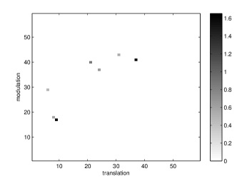
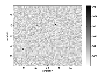
But before doing so, we illustrate in Figure 1 the recovery method for matrices which have a sparse representation in the dictionary of time–frequency shift matrices as considered in Theorem 2.5. A $7$-sparse coefficient vector $\bm{x}$ in the time-frequency plane is chosen and reconstructed from $\bm{\Gamma}\bm{h}^{A}=\sum_{\ell,p}x_{\ell p}\bm{M}_{\ell}\bm{T}_{p}\bm{h}^{A}$ by Basis Pursuit. As comparison, $\bm{x}$ is reconstructed by a traditional reconstruction by $\ell_{2}$-minimization,

$$\min\|\bm{x}\|_{2}\text{ subject to }(\bm{\Psi}\bm{h}^{A})x=\bm{\Gamma}\bm{h}^{A}\,.$$ (28)

(a)

(b)

(c)

Figure 1: (a) Original $7$-sparse coefficient vector ($n=59$) in the time-frequency plane. (b) Reconstruction by Basis Pursuit using the Alltop window $\bm{h}^{A}$. (c) For comparison, the reconstruction by traditional $\ell_{2}$-minimization (28).

For the Alltop window $\bm{h}^{A}$ in (7) we consider the values of $n$ prime from 11 to 59, for the random window $\bm{h}^{R}$ in equation (8) we consider the values of $n$ prime from 11 to 59 as well as $n=10+4j$ for $j=0,1,\ldots,12$. Each empirical test consists of generating a random $k$-sparse $x\in{\mathbb{C}}^{n^{2}}$ with non-zero entries $x_{q}=r_{q}\exp(2\pi i\theta_{q})$, with $r_{q}$ drawn independently from the Gaussian $N(0,1)$ distribution, and $\theta_{q}$ drawn independently and uniformly from $[0,1)$.

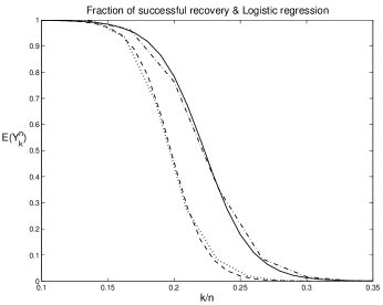
For each value of $n$, 1000 tests are computed per value of $k=1,2,\ldots,n{-}1$. A test is considered successful if Basis Pursuit (3) recovers all components of the coefficient vector $\bm{x}$ with $10^{-10}$ error tolerance. The successful recovery of $\bm{x}$, and, hence, of $\bm{\Gamma}$ from $\bm{\Gamma}\bm{h}^{A}$ or $\bm{\Gamma}\bm{h}^{R}$ is recorded in $Y_{k}^{n}$ as a 1, and failure to recover as a 0. Following the empirical examination of phase transitions in [18], we approximate the observed probability distribution by fitting the mean response of $Y_{k}^{n}$ using the logistic regression model, [31],

$$E(Y_{k}^{n})=\frac{\exp(\beta_{0}(n)+\beta_{1}(n)k)}{1+\exp(\beta_{0}(n)+\beta_{1}(n)k)}.$$ (29)

For illustration purposes, the fitted response for windows $\bm{h^{A}}$ with $n=43$ and $\bm{h^{R}}$ with $n=30$ is shown in Figure 2 along with the mean response of $Y_{k}^{n}$.

Figure 2: Empirical verification of Theorem 2.5 without noise. For the random window $\bm{h}^{R}$ with $n=30$ the mean response of $Y_{k}^{n}$ (dash-dot) and fitted logistic regression model $E(Y^{n}_{k})$, (solid), plotted against the fractional sparsity $k/n$. For the Alltop window $\bm{h}^{A}$ with $n=43$ the mean response of $Y_{k}^{n}$ (dot) and fitted logistic regression model $E(Y^{n}_{k})$, (dash), plotted against the fractional sparsity $k/n$.

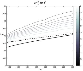
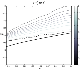
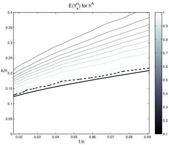
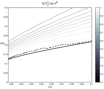
The phase transition behaviors are often observed through the fractional sparsity ratio $k/n$, and the matrix so-called undersampling rate $n/N$, here $1/n$ for $\bm{\mathcal{G}}\bm{h}^{A}$ and $\bm{\mathcal{G}}\bm{h}^{R}$ [24]. Contours of the fitted logistic regression models for time-frequency shift dictionaries with identifiers $\bm{h}^{A}$ and $\bm{h}^{R}$ are shown in Figure  3 (a) and (b) respectively. To facilitate a quantitative inspection of the contours in Figure 3 and the theoretical results of [24] we overlay the contours in Figure 3 with the level curve for $93\%$ success rate (dash) and $1/(2\log n)$ (solid). The curve $1/(2\log n)$ is known to be the threshold for overwhelming probability of successful recovery in the case of Gaussian random matrices for large $n$ [24]. It is observed in Figure 3 that the curve $1/(2\log n)$ remains below the $93\%$ success rate level curve, indicating consistence of the empirical results with the phase transition $1/(2\log n)$ conjectured for the class of time-frequency shift matrices applied to identifiers $\bm{h}^{A}$ and $\bm{h}^{R}$. Moreover, the curve $1/(2\log n)$ increasingly falls below the $93\%$ success rate level curve as $n$ increases, indicating improved agreement in the large $n$ limit. Note that this conjectured phase transition $1/(2\log n)$ is larger than that proven in the main Theorem  2.5, both in order (as $u=0$ here), as well as in the constant.

(a)

(b)

Figure 3: Empirical verification of Theorem 2.5 for $\bm{h}^{A}$ (a) and $\bm{h}^{R}$ (b) without noise. Contours of the fitted logistic regression model (gray), the $93\%$ success rate contour (dashed), and $1/(2\log n)$ (solid). Figure 2 shows vertical slices for $1/43$ (a) and $1/30$ (b).

As stated earlier, in practice the measurements $\bm{\Gamma}\bm{h}$ are observed with noise and although $\bm{\Gamma}$ can be well approximated by a $k$-sparse representation, it is rarely strictly $k$-sparse. For both of these reasons, the recovery algorithm (3) is not often used in practice, rather (4) is used to allow for an inexact fit of the measurements.

In Figure 4 we empirically test Theorem 2.5 using (4) rather than (3) for the reconstruction algorithm. We choose the same values of $k$ and $n$, and the same number of tests were performed as for Figure 3. The non-zero entries in $\bm{x}$ are also selected from the same distribution as was used to generate Figure 3. Additive noise is simulated at a level of 25 dB signal to noise ratio; that is, $\bm{\eta}$ is added to $\bm{\Gamma}\bm{h}$ with the entries in $\bm{\eta}$ drawn independently from the Gaussian $N(0,1)$ and $\bm{\eta}$ is normalized to $\|\bm{\eta}\|_{2}=\|\bm{\Gamma}\bm{h}\|_{2}\cdot 10^{-5/4}$.

(a)

(b)

Figure 4: Empirical verification of Theorem 2.5 for $\bm{h}^{A}$ (a) and $\bm{h}^{R}$ (b) in the noisy setting, with (3) replaced by (4) and additive noise of $25$ dB signal to noise ratio. Contours of the fitted logistic regression model (gray), the $93\%$ success rate contour (dash), and $1/(2\log n)$ (solid).

Unlike the solution of (3) for which the exact solution can be exactly $k$-sparse, and for which numerical algorithms can compute approximations of arbitrary precision, the solution of (4) from noisy measurements will not recover the solution exactly. For our numerical experiments involving noisy measurements, the vector $\bm{x}$ associated with $\bm{\Gamma}$ resulting from the solution of (4) is only considered to have been successfully recovered if the largest $k$ entries of the recovered $\bm{x}^{\prime}$ have the same support set $\Lambda$ as $\bm{x}$. Alternative metrics of successful recovery, such as $\ell^{2}$ error or Signal to Noise Ratio (SNR), are less demanding than requiring a match of the support set; moreover, the support set metric was previously examined in this setting by Wainwright [55] and following this convention allows for a more direct comparison. The inequality fit parameter $\epsilon$ in (4) is selected to be at the noise level $10^{-5/4}$.

As in the noiseless setting, we approximate the probability distribution of the empirical observations $Y_{k}^{n}$ using the logistic regression model (29). Contours of the fitted logistic regression models for time-frequency shift dictionaries with identifiers $\bm{h}^{A}$ and $\bm{h}^{R}$ are shown in Figure 4 (a) and (b) respectively. Overlaying these contours is the level curve for $93\%$ success rate (dash) and $1/(2\log n)$ (solid). Unlike the noiseless case (3), it was shown that the threshold for overwhelming probability of successful recovery in the case of Gaussian random $n\times n^{2}$ matrices with noise using (4) is $1/(4\log n)$, [55]; however, we observe in Figure 4 that $1/(2\log n)$ fits the empirical data better in this instance. As Wainwright considered the Gaussian setting, this empirical observation for the Gabor system does not contradict results in [55], but the difference is noteworthy.

In Figure 5 we illustrate the performance of Basis Pursuit when using multiple test signals as discussed in Section 6, in particular in Theorem 6.3. Figure 5 was obtained using the same procedure that provided Figure 2.

Figure 5: Empirical verification of Theorem 6.3 without noise. For the random windows $\bm{h}_{1}^{R},\bm{h}_{2}^{R},\bm{h}_{3}^{R}$ with $n=30$ the fraction of successful recovery based on $\bm{\mathcal{G}}\bm{h}_{1}^{R}$ (dash-dot), $\bm{\mathcal{G}}\bm{h}_{1}^{R}$ and $\bm{\mathcal{G}}\bm{h}_{2}^{R}$ (solid), and $\bm{\mathcal{G}}\bm{h}_{1}^{R}$, $\bm{\mathcal{G}}\bm{h}_{2}^{R}$ and $\bm{\mathcal{G}}\bm{h}_{3}^{R}$ (dash) test vectors.

References

- [1] D. Achlioptas. Database-friendly random projections. In Proc. 20th Annual ACM SIGACT-SIGMOD-SIGART Symp. on Principles of Database Systems, pages 274–281, 2001.
- [2] M. Akcakaya and V. Tarokh. Performance bounds on sparse representations using redundant frames. Preprint, 2007.
- [3] W. O. Alltop. Complex sequences with low periodic correlations. IEEE Trans. Inf. Theory, 26(3):350–354, 1980.
- [4] R. Baraniuk, M. Davenport, R. DeVore, and M. Wakin. A simple proof of the restricted isometry property for random matrices. Constr. Approx., to appear.
- [5] P. Bello. Characterization of randomly time-variant linear channels. IEEE Trans. Commun., 11:360–393, 1963.
- [6] S. Boyd and L. Vandenberghe. Convex Optimization. Cambridge Univ. Press, 2004.
- [7] E. Candès, J. Romberg, and T. Tao. Robust uncertainty principles: exact signal reconstruction from highly incomplete frequency information. IEEE Trans. Inf. Theory, 52(2):489–509, 2006.
- [8] E. Candès, J. Romberg, and T. Tao. Stable signal recovery from incomplete and inaccurate measurements. Comm. Pure Appl. Math., 59(8):1207–1223, 2006.
- [9] E. Candès and T. Tao. Near optimal signal recovery from random projections: universal encoding strategies? IEEE Trans. Inf. Theory, 52(12):5406–5425, 2006.
- [10] I. Cavdar. Performance analysis in non-Rayleigh and non-Rician communication channels. Computers & Electrical Engineering, 28.
- [11] M. Cetin and B. Sadler. Semi–blind sparse channel estimation with constant modulus symbols. In Proc. IEEE ICASSP 05, volume 3, pages iii/561– iii/564, Atlanta (GA), 2005.
- [12] O. Christensen. An introduction to frames and Riesz bases. Applied and Numerical Harmonic Analysis. Birkhäuser Boston Inc., Boston, MA, 2003.
- [13] L. M. Correia. Wireless Flexible Personalized Communications. John Wiley & Sons, Inc., New York, NY, USA, 2001.
- [14] S. Cotter and B. Rao. Sparse channel estimation via matching pursuit with applications to equalization. IEEE Trans. on Comm., 50(3):374–377, 2002.
- [15] D. Donoho. Compressed sensing. IEEE Trans. Inf. Theory, 52(4):1289–1306, 2006.
- [16] D. Donoho, I. Drori, J.-L. Starck, and Y. Tsaig. Sparse solution of underdetermined linear equations by stagewise orthogonal matching pursuit. Preprint, 2006.
- [17] D. Donoho and J. Tanner. Sparse nonnegative solutions of underdetermined linear equations by linear programming. Proc. Nat. Acad. Sci., 102(27):9446–9451, 2005.
- [18] D. Donoho and Y. Tsaig. Fast solution of l1-norm minimization problems when the solution may be sparse. Preprint, 2006.
- [19] D. L. Donoho. Neighborly polytopes and sparse solutions of underdetermined linear equations. Preprint, 2005.
- [20] D. L. Donoho. High-dimensional centrally symmetric polytopes with neighborliness proportional to dimension. Discrete Comput. Geom., 35(4):617–652, 2006.
- [21] D. L. Donoho and M. Elad. Optimally sparse representations in general (non-orthogonal) dictionaries via minimization. Proc. Nat. Acad. Sci., 100:2197–2202, 2002.
- [22] D. L. Donoho, M. Elad, and V. N. Temlyakov. Stable recovery of sparse overcomplete representations in the presence of noise. IEEE Trans. Inf. Theory, 52(1):6–18, 2006.
- [23] D. L. Donoho and J. Tanner. Neighborliness of randomly projected simplices in high dimensions. Proc. Natl. Acad. Sci. USA, 102(27):9452–9457, 2005.
- [24] D. L. Donoho and J. Tanner. Counting faces of randomly-projected polytopes when the projection radically lowers dimension. Preprint, 2006.
- [25] P. Georgiev and A. Ralescu. Clustering on subspaces and sparse representation of signals. Circuits and Systems, 2:1843–1846, 2005.
- [26] A. Gilbert and J. Tropp. Signal recovery from random measurements via orthogonal matching pursuit. IEEE Trans. Inform. Theory, to appear.
- [27] R. Gribonval and P. Vandergheynst. On the exponential convergence of matching pursuits in quasi-incoherent dictionaries. IEEE Trans. Inform. Theory, 52(1):255–261, 2006.
- [28] N. Grip and G. Pfander. A discrete model for the efficient analysis of time-varying narrowband communication channels. Multidim Syst Sign P, to appear.
- [29] K. Gröchenig. Foundations of Time-Frequency Analysis. Applied and Numerical Harmonic Analysis. Birkhäuser, Boston, MA, 2001.
- [30] D. Han, S.-P. Kim, and J. Principe. Sparse channel estimation with regularization method using convolution inequality for entropy. In Proc. IJCNN’05, International Joint Conf. on Neural Networks, volume 4, pages 2359–2362, August 2005.
- [31] T. Hastie, R. Tibshirani, and J. Friedman. The Elements of Statistical Learning. Springer, 2001.
- [32] M. Herman and T. Strohmer. High resolution radar via compressed sensing. Preprint, 2007.
- [33] S. Kim, K. Ksh, M. Lustig, S. Boyd, and D. Gorinevsky. A method for large-scale l1-regularized least squares problems with applications in signal processing and statistics. Preprint, 2007.
- [34] W. Kozek and G. Pfander. Identification of operators with bandlimited symbols. SIAM J. Math. Anal., 37(3):867–888, 2006.
- [35] F. Krahmer, G. Pfander, and P. Rashkov. Uncertainty principles for time–frequency representations on finite abelian groups. 2006.
- [36] S. Kunis and H. Rauhut. Random sampling of sparse trigonometric polynomials II - orthogonal matching pursuit versus basis pursuit. Found. Comput. Math., to appear.
- [37] J. Lawrence, G. Pfander, and D. Walnut. Linear independence of Gabor systems in finite dimensional vector spaces. J. Fourier Anal. Appl., 11(6):715–726, 2005.
- [38] M. Ledoux and M. Talagrand. Probability in Banach Spaces. Isoperimetry and Processes. Springer-Verlag, Berlin, Heidelberg, New York, 1991.
- [39] D. Middleton. Channel modeling and threshold signal processing in underwater acoustics: An analytical overview. IEEE J. Oceanic Eng., 12(1):4–28, 1987.
- [40] J. Parsons, D. Demery, and A. Turkmani. Sounding techniques for wideband mobile radio channels: a review. IEE Proceedings-1, 138(5):437–446, 1991.
- [41] M. Pätzold. Mobile Fading Channels: Modelling,Analysis and Simulation. John Wiley & Sons, Inc., New York, NY, USA, 2001.
- [42] G. Pevskir and A. Shiryaev. The Khintchine inequalities and martingale expanding sphere of their action. Russ. Math. Surv., 50(5):849–904, 1995.
- [43] G. Pfander and D. Walnut. Measurement of time–variant channels. IEEE Trans. Info. Theory, 52(11):4808–4820, 2006.
- [44] H. Rauhut. Stability results for random sampling of sparse trigonometric polynomials. Preprint, 2006.
- [45] H. Rauhut. Random sampling of sparse trigonometric polynomials. Appl. Comput. Harm. Anal., 22(1):16–42, 2007.
- [46] H. Rauhut, K. Schnass, and P. Vandergheynst. Compressed sensing and redundant dictionaries. Preprint, 2006.
- [47] M. Rudelson and R. Vershynin. Sparse reconstruction by convex relaxation: Fourier and Gaussian measurements. In Proc. CISS 2006 (40th Annual Conference on Information Sciences and Systems), 2006.
- [48] S. Sanyal, S. Kukreja, E. Perreault, and D. Westwick. Identification of linear time varying systems using basis pursuit. In Proceedings of the IEEE EMBS 2005.
- [49] M. Skolnik. Introduction to Radar Systems. McGraw-Hill Book Company, New York, 1980.
- [50] M. Stojanovic. Underwater Acoustic Communications, volume 22, pages 688–698. John Wiley & Sons, 1999.
- [51] T. Strohmer and R. W. Heath. Grassmannian frames with applications to coding and communication. Appl. Comput. Harmon. Anal., 14(3):257–275, 2003.
- [52] J. Tropp. Greed is good: Algorithmic results for sparse approximation. IEEE Trans. Inf. Theory, 50(10):2231–2242, 2004.
- [53] J. A. Tropp. Just relax: Convex programming methods for identifying sparse signals. IEEE Trans. Inf. Theory, 51(3):1030–1051, 2006.
- [54] J. A. Tropp. On the conditioning of random subdictionaries. Appl. Comput. Harmon. Anal., to appear.
- [55] M. J. Wainwright. Sharp thresholds for noisy and high-dimensional recovery of sparsity using -constrained quadratic programming. Preprint, 2006.