Noise Robust Online Inference for Linear Dynamic Systems

Abstract

We revisit the Bayesian online inference problems for the linear dynamic systems (LDS) under non-Gaussian environment. The noises can naturally be non-Gaussian (skewed and/or heavy tailed) or to accommodate spurious observations, noises can be modeled as heavy tailed. However, at the cost of such noise robustness, the performance may degrade when such spurious observations are absent. Therefore, any inference engine should not only be robust to noise outlier, but also be adaptive to potentially unknown and time varying noise parameters; yet it should be scalable and easy to implement.

To address them, we envisage here a new noise adaptive Rao-Blackwellized particle filter (RBPF), by leveraging a hierarchically Gaussian model as a proxy for any non-Gaussian (process or measurement) noise density. This leads to a conditionally linear Gaussian model (CLGM), that is tractable. However, this framework requires a valid transition kernel for the intractable state, targeted by the particle filter (PF). This is typically unknown. We outline how such kernel can be constructed provably, at least for certain classes encompassing many commonly occurring non-Gaussian noises, using auxiliary latent variable approach. The efficacy of this RBPF algorithm is demonstrated through numerical studies.

I Introduction

Many applications of interest to the signal processing community (e.g., tracking, autonomous navigation and surveillance) require that the inference must be performed on near real-time (online) using the streaming sensor data. The stability and the performance of the underlying inference engines however depend crucially on the sensor data quality. Usually, any spurious sensor data needs to be detected and discarded before passing to the inference engine, so that the latter is not susceptible to permanent failure. In recent times, the sensors are becoming cheaper, however at the expense of their performance reliability. The proliferation of such inexpensive sensors has opened up the possibility to explore many complex and high dimensional problems (e.g., motion tracking, road traffic monitoring), which are hitherto impossible with a limited number of costly sensors. This trend for using inexpensive sensors has in turn, laid greater emphasis on the processing algorithms to the extent that any inference algorithm (presumably with more computing prowess) is required to be robust and stable against such spurious sensor data; yet simple to implement and vastly scalable to the high dimensional problems. Against this backdrop, we consider the online inference problems for the discrete time LDS.

I-A Problem Background

Consider the following discrete time LDS relating the latent state $x_{k}\in\mathbb{R}^{n_{x}}$ at time step $k$ to the observation $y_{k}\in\mathbb{R}^{n_{y}}$ as

$$x_{k} =A_{k}\ x_{k-1}+B_{k}\ w_{k},$$ (1a)

$$y_{k} =C_{k}\ x_{k}+e_{k},$$ (1b)

where $w_{k}$ and $e_{k}$ are the process and measurement noise respectively. The noises are assumed to be independent and also independent of each other. The model parameters $\{A_{k},B_{k},C_{k}\}$ are considered to be known here. Given this model, an initial state prior (i.e., $p(x_{0})$) and a stream of observations up to time $k$, $y_{0:k}\triangleq\{y_{0},y_{1},\dots,y_{k}\}$, one typical inference task is to optimally estimate the sequence of (posterior) densities $p(x_{k}|y_{1:k})$, in an online fashion over time. This is known as the online Bayesian filtering problem for the LDS, and the density $p(x_{k}|y_{1:k})$ is called as the filtering density. When the noises above are Gaussian, the filter density can be obtained recursively in closed form using the celebrated Kalman filter (KF)[West_h97, Bagchi, Anderson_79]. However, this analytical tractability is lost if any noise deviates from such nominal Gaussian assumptions.

In reality, many noise sources naturally appear to be non-Gaussian (characterized by their heavy tails and/or skewness). For example, noise with an impulsive nature (sharp spikes and/or occasional bursts) appears in many applications such as speech and audio signal processing, astrophysical imaging, underwater navigations, multi-user radar communications, kick detection in oil drilling, finance and insurance among others [Chenssp14, Jordi14, ZoubirSPM, Mila_stable, Hawary95, Godsill96, Fruhwirth07, Adler98]. This impulsive nature can be modeled e.g., by a noise distribution that has heavier tails than the Gaussian distribution. Heavy tailed distributions are also used to model the presence of so called outliers, which are data points, that do not appear to follow the pattern of the other data points [Ross]. Data from the visual sensors, GPS devices, sonar, and radar are often contaminated by such outliers. The root causes of such outlying observations are often unknown or are excluded deliberately from the model due to the complexity and the computational issues. So under such simplified modeling of complex real world processes, these unusual observations can be taken care by noise outliers. This in turn, requires heavy tailed distributions for the noises[Pearson02].

In the filtering context, when a nominal model with specified Gaussian noises cannot account for the outliers or sudden change in unknown input signals, the filter becomes unstable. Since for the real world applications, often we have weak knowledge on the systems and outliers are frequent, naturally, the filtering problems under heavy tailed noises have attracted considerable research attentions [Agamennoni11, Piche_SS_JH12, Roth_Lic, Ting_ecml07]. We note that in the context of filtering, the process and/or the observation noise can have heavy tails. Although heavy tailed observation noise have received much attention, in applications like maneuvering target tracking, modeling occasional pilot induced changes requires a heavy tailed process noise [Sinha_TAES]. In contrast, although skewness appears in many applications [Kok_Lic], the associated online inference problem has not been well explored .

Non-Gaussian noise can also appear due to the modeling artifact. We illustrate the last point through the following example:

I-A1 Stochastic volatility model

We consider the following discrete time model [Shephard96]

$$h_{k+1} =\gamma_{0}+\gamma_{1}h_{k}+\eta_{k},$$ (2a)

$$y_{k} =\epsilon_{k}exp(h_{k}/2),$$ (2b)

where $h_{k}$ and $y_{k}$ are the latent log-volatility and observed asset return at time step $k$ with $|\gamma_{1}|<1$, $h_{0}\sim\mathcal{N}(0,\frac{\sigma_{n}^{2}}{1-\gamma_{1}^{2}})$, $\eta_{k}\stackrel{{\scriptstyle iid}}{{\sim}}\mathcal{N}(0,\sigma_{n}^{2})$ and $\epsilon_{k}\stackrel{{\scriptstyle iid}}{{\sim}}\mathcal{N}(0,1)$, where iid means independent and identically distributed. $\gamma_{0},\gamma_{1}$ and $\sigma_{n}$ are assumed to be known. Here $\eta_{k}$ is uncorrelated to $\epsilon_{k}$, i.e. no leverage effect is considered. Note that the measurement noise is multiplicative. The above dynamic model can equivalently be cast as a linear state space model:

$$h_{k+1} =\gamma_{0}+\gamma_{1}h_{k}+\eta_{k},$$ (3a)

$$log(y_{k}^{2}) =h_{k}+log(\epsilon_{k}^{2}).$$ (3b)

However the observation noise $e_{k}\equiv log(\epsilon_{k}^{2})$, being log of a $\chi^{2}$ random variable, is no more Gaussian. In fact, the density of this noise is available analytically, given by (see e.g.,[Douc14])

$$f(e_{k})=\frac{1}{\sqrt{2\pi}}{exp\big{\{}-0.5\big{(}exp(e_{k})-e_{k}\big{)}\big{\}}},\ -\infty<e_{k}<\infty.$$ (4)

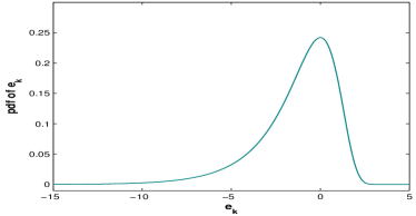
Figure 1: Density plot for the observation noise in (4).

From Figure (1), it is evident that the density is highly skewed. Thus, we have a LDS driven by a non-Gaussian (measurement) noise.

While the noise distribution is certainly a key factor for the inference task, the other equally important aspect for practical considerations is the knowledge on the noise statistics. In many practical contexts, although prior knowledge on the noise distributions is fairly available, the corresponding noise parameters are often unknown. Thus additionally, the noise parameters need to be estimated on the fly as well. This is known as online noise adaptive filtering. When the noise parameters are stationary, the online Bayesian estimation of the parameters is known to be difficult and one practical solution is to assume the noise parameters to be slowly varying in time[OzkanSSLG13]. However, this assumption easily breaks down in the presence of any potential outlier. To get rid of the outliers, some mechanisms are usually placed to detect and immediately discard them. However such outlying observations may carry important information about e.g., any unmodeled system characteristics and model degradation and as such, as pointed out in [Cappe05], ”Routinely ignoring unusual observations is neither wise nor statistically sound”. On the other hand, eventhough such outliers can be accommodated by using e.g., a properly specified heavy tailed noise distribution from a known parametric family, the performance of the filter can be degraded severely when the outliers are absent. This happens due to the use of fixed form of distribution. To alleviate this problem in noise adaptive filtering, essentially what we need is to use a heavy tailed noise, whose parameters are time varying. However, coping with nonstationary noise parameters in online setting is very challenging as the corresponding dynamics for the parameters cannot be easily specified a priori in practice.

I-B Prior works

There is a long history on the efforts of improving the KF algorithm under the non-Gaussian environments. The earlier attempts were mainly based on the robustification arguments in the presence of outliers. These were primarily addressed either by analytical approximations using elliptical noise distributions or by heuristic cost functions in the update step of KF. The elliptical noise based approaches [Meinhold89, Giron94] were not robust, as the posterior mean is unbounded as a function of the residuals, whereas the approaches based on the ad-hoc cost functions (e.g., [Masreliez75, Durovic]) requires tuning of parameters and their implementations were very involved as compared to KF. Later, the simulation based approaches (e.g., PF)[DelMoral04, Cappe05] became popular due to their ease of implementations. However, the major disadvantages were their non-scalability together with computational costs[Snyder08]. Several recent articles have addressed the filtering problem using variational Bayes (VB) [Ting_ecml07, Agamennoni11, Piche_SS_JH12] and convex optimization based methods [Boyd]. Although VB method is quite scalable, in general, it requires fairly involved mathematical derivations and is known to consistently underestimate the posterior covariance. Common to all these recent studies is the assumption of outliers in the observation noise only. The methods by [Ting_ecml07, Piche_SS_JH12, Boyd] do not accommodate any persistence (time correlated) noise outliers. Moreover, [Piche_SS_JH12] considers a heuristic transition model for the noise parameter (as observed by [Agamennoni11], the filter is not stable under abrupt change in noise) whereas [Agamennoni11, Boyd] require additional input parameter from the user. More recently, observing that the VB based algorithms are very sensitive to process noise outlier, [Roth_Lic] proposed an analytical approximation based t filter, where both the process and observation noises are Students’ t. The approximations here require that the estimated state and process/observation noise is jointly t with a common degree of freedom (dof) parameter. To maintain these hypotheses and to prevent the growth of dof parameters in filter recursion, again careful tuning is required at each step. For all the cases, the noise class is implicitly assumed to be symmetric and Students’ t.

From the literature above, we see that many of the existing approaches require manual tuning of the parameters and also their implementations are substantially involved as compared to well understood KF. Thus any future inference framework should ideally be free of such heuristic tuning and the implementation should be simple to understand. Also, any future framework should be able to handle-(a) asymmetric noise and (b) symmetric heavy tailed noise other than Students’ t.

I-C Sketch of our contributions

Keeping in view the points above, we consider the online inference for the LDS under a fairly general and realistic scenario. This is addressed here in two stages by successively dropping the following common assumptions: (a) noises are Gaussian and (b) noise parameters are known.

In the first stage, we consider the LDS under (known) stationary non-Gaussian environment. The corresponding inference task is analytically intractable. In our approach, we envisage a hierarchically Gaussian model (HGM) as a proxy for any non-Gaussian noise. This model can represent the skewness and/or heavy tail that are typical characteristics of the non-Gaussian noise. Such representation allows us to exploit a CLGM, which is analytically tractable using a KF. This in turn, leads to a RBPF framework for the online inference task. Since within the RBPF framework, PF is confined to a space of lower dimension, it acts as an enabler for scaling to high dimensional problems. The proposed framework here uses a bank of KFs, which is simple to understand; the sophistication comes in the way how we mix and propagate the output of different KFs to get the target filter density. Although this RBPF framework is not entirely new [chen:liu:00:mixture], a proper specification of the transition kernel for the state, targeted by PF is often difficult and this technical aspect has received little attention. We elaborate this issue in details and address the proper transition kernel for certain class of noises (where widely used Students’ t is a special case).

For the second stage, we point how this RBPF framework is already doing a noise adaptive filtering. However to make the filter robust against any large noise deviation, we need prior knowledge about such deviation. Often this is reasonably well known for many practical applications. For such cases, we outline how this information can be encoded in the noise prior. This completes our noise robust online inference framework.

I-D Organization of the article

The rest of the article is organized as follows. We start with brief descriptions on HGM in section II and simulation based online filtering in section III. This is then followed by the development of the proposed inference framework for LDS under stationary non-Gaussian environment in section LABEL:LDS_inf. We then describe how the above framework can be used for robust noise adaptive filtering in section LABEL:rob_noise_adap. Subsequently, the numerical experiments are shown in LABEL:num_experiment, which is followed by concluding remarks in section LABEL:conclusion.

II Hierarchical Gaussian model (HGM) for non-Gaussian density

Non-Gaussian densities are often characterized by the presence of heavy tail and/or skewness. Many such densities can often be modeled as hierarchically Gaussian. That is, the density can be represented as Gaussian, conditionally on an auxiliary random variable, known as the ’mixing parameter’. We outline below a brief description for such hierarchical Gaussian representation. For the clarity of the presentation, we consider two separate classes based on the symmetry of underlying density. When the density is symmetric, HGM is represented as scale mixture of normal (SMN), also known as normal variance mixture (NVM). For the non symmetric density, it is represented as normal variance-mean mixture (NVMM) model.

II-A Scale mixtures of normal

A random vector $X$ has a scale mixtures of normal density, if it can be expressed as follows

$$X=\mu+\kappa^{\frac{1}{2}}(\Lambda)Z,$$ (5)

where $\mu$ is a location vector, $Z$ is distributed according to a zero mean multivariate normal with covariance matrix $\Sigma$ and $\kappa$ is a positive weight function. $\Lambda$ is a random variable, known as mixing parameter and is distributed on the positive real line, independent of $Z$. Note here that conditioned on $\Lambda=\lambda$, $X$ follows a multivariate normal distribution with mean vector $\mu$ and covariance matrix $\kappa(\lambda)\Sigma$, i.e., $(X|\Lambda=\lambda)\sim{\cal N}(x|\mu,\kappa(\lambda)\Sigma)$. Then, the probability density function (pdf) of $X$ can be expressed as

$$p(x)=\int_{0}^{\infty}{\cal N}(x|\mu,\kappa(\lambda)\Sigma)p(\lambda)d\lambda,$$ (6)

where $p(\lambda)$ is the density function of $\Lambda$. $p(\lambda)$ is referred to as the mixing density of SMN representation.

The symmetrical class of SMN includes among others, the popular Students’ t, the Pearson type VII family, the Slash and the variance gamma distributions. All these distributions are characterized by their heavy tails as compared to the normal distribution. Although there exists many other important SMN distributions (e.g., exponential power, symmetric $\alpha$ -stable, logistic, horse shoe, symmetric generalized hyperbolic distribution)[ChoyChan08, carvalho2010], in the sequel, we present only the above mentioned special cases, as the associated mixing densities have computationally attractive form.

II-A1 Multivariate Students’ t distribution

When $X$ follows a multivariate Students’ t distribution with location $\mu$, scale $\Sigma$ and degrees of freedom $\nu$ (i.e., $X\sim\mathcal{T}(\mu,\Sigma;\nu)$), the pdf of $X$ can be expressed in the following SMN form

$$p(x)=\int_{0}^{\infty}{\cal N}(x|\mu,\frac{\Sigma}{\lambda})Ga(\lambda|\frac{\nu}{2},\frac{\nu}{2})d\lambda,$$ (7)

where $Ga(\cdot|a,b)$ is the gamma density function of the form

$$Ga(\lambda|a,b)=\frac{b^{a}}{\Gamma(a)}\lambda^{a-1}e^{-b\lambda},\ \ \lambda,a,b>0,$$ (8)

and $\Gamma(a)$ is the gamma function with argument $a>0$. Consequently, $X$ can be presented in the following hierarchical form

$$X|(\mu,\Sigma,\nu,\lambda)\sim{\cal N}(\mu,\lambda^{-1}\Sigma),\ \ \lambda|\nu\sim Ga(\frac{\nu}{2},\frac{\nu}{2}).$$ (9)

II-A2 Pearson type VII distribution

If $X$ belongs to the Pearson type VII family, the associated density is given by

$$p(x|\mu,\Sigma,\nu,\delta)=\frac{1}{B(\frac{\delta}{2},\frac{1}{2})\sqrt{\nu\Sigma}}\big{(}1+\frac{(x-\mu)^{2}}{\nu\Sigma}\big{)}^{-(\delta+1)/2},$$ (10)

where $\mu$ and $\Sigma$ are the location and scale parameters, $\nu>0$ and $\delta>0$ are the shape parameters and $B(a,b)$ is the beta function with arguments $a>0$ and $b>0$. The Pearson type VII density can be expressed hierarchically as

$$X|(\mu,\Sigma,\nu,\delta,\lambda)\sim{\cal N}(\mu,\lambda^{-1}\Sigma),\ \ {\lambda}|(\nu,\delta)\sim Ga(\frac{\nu}{2},\frac{\delta}{2}).$$ (11)

We get back to Students’t distribution when $\nu=\delta$ and Cauchy if $\nu=\delta=1$.

II-A3 Multivariate slash distribution

The Slash distribution can be hierarchically represented as

$$X|(\mu,\Sigma,\nu)\sim{\cal N}(\mu,\lambda^{-1}\Sigma),\ \ \lambda|\nu\sim Be(\nu,1),$$ (12)

with $0<\lambda<1$ and $\nu>0$, where $Be(\cdot)$ denotes the Beta distribution.

II-A4 Multivariate variance gamma distribution

When $X$ follows a multivariate variance gamma (VG) distribution with location $\mu$, scale $\Sigma$ and degrees of freedom $\nu>0$ (i.e., $X\sim\mathcal{VG}(\mu,\Sigma;\nu)$), the density can be represented in the following hierarchical form

$$X|(\mu,\Sigma,\nu,\lambda)\sim{\cal N}(\mu,\lambda^{-1}\Sigma),\ \ \lambda|\nu\sim IG(\frac{\nu}{2},\frac{\nu}{2}),$$ (13)

where $IG(a,b)$ is the inverse gamma density given by

$$IG(\lambda|a,b)=\frac{b^{a}}{\Gamma(a)}\lambda^{-(a+1)}e^{-b/\lambda}.$$ (14)

When $\nu=2$, VG turns into a Laplace distribution.

II-B Normal variance-mean mixture

A random vector $X$ is following a normal variance-mean mixture distribution, if it can be expressed as follows [Nielsen82]

$$X=\mu+\beta\Lambda+\sqrt{\Lambda}Z,$$ (15)

where $\Lambda$ is independent of $Z$ and $Z$ is distributed according to a zero mean multivariate normal with covariance matrix $\Sigma$. The random variable $\Lambda$ is the mixing parameter and is distributed on the positive real line and $\mu,\beta\in\mathbb{R}$. The distribution of $X$ conditioned on $\Lambda=\lambda$ is multivariate normal given as $(X|\Lambda=\lambda)\sim{\cal N}(x|\mu+\beta\lambda,\Sigma\lambda)$. Note that when $\beta=0$, the NVMM turns into a SMN with $\kappa(\lambda)=\lambda$. We describe below some special cases of this class of distributions:

II-B1 Generalized hyperbolic distribution

$X$ in (15) follows a generalized hyperbolic (GH) distribution, if $\Lambda$ is distributed according to a generalized inverse Gaussian (GIG) distribution as

$$p(\lambda)=\frac{(a/b)^{p/2}}{2K_{p}(\sqrt{ab})}\lambda^{p-1}exp\{-\frac{a\lambda+b/\lambda}{2}\},\ \lambda>0,$$ (16)

where $K_{p}$ is the modified Bessel function of the second kind, $a,b\in\mathbb{R}^{+}$, and $p\in\mathbb{R}$.

II-B2 GH skew Students’ t distribution

The hierarchical structure of GH skew Students’ t distribution is given as [Nakajima:csda12]

$$(X|\Lambda=\lambda)\sim{\cal N}(x|\mu+\beta\lambda,\Sigma\lambda),\ \lambda|\nu\sim IG(\nu/2,\nu/2),$$ (17)

where inverse-gamma density is given by (14). Note that the GH skew Students’ t is a special case of the GH distribution, where the parameters for the GIG are selected as $a=-\nu/2\ (\nu>0)$, $b=\sqrt{\nu}$ and $p=0$. Moreover, when $\beta=0$, this turns to a symmetric Students’ t distribution and if $\nu\rightarrow\infty$, this becomes a skew normal distribution.

II-B3 GH variance gamma distribution

The hierarchical structure of GH variance gamma distribution is given as

$$(X|\Lambda=\lambda)\sim{\cal N}(x|\mu+\beta\lambda,\Sigma\lambda),\ \lambda|\nu\sim Ga(\nu/2,\nu/2),$$ (18)

where the gamma density is given by (8).

Remark 1

note that the mixing parameter $\Lambda$ in II-A and II-B being a random variable, dimension of $\Lambda$ is always less than or equal to that of random vector $X$. This observation is important, as we will see later that the PF can be used to target the low dimensional $\Lambda$ in a RBPF framework.

III Simulation based online filtering

When a dynamic system (state space model) is nonlinear and/or driven by non-Gaussian noises, the filter density $p(x_{k}|y_{1:k})$ is in general, analytically intractable. To deal with, many approximated methods have been proposed over time [Murphy_book]. Particle filtering (PF) is one such method, which uses Monte Carlo simulations to address the filtering problem. In this section, we give a very brief overview of PF and RBPF.

III-A Particle filtering (PF)

In PF, the posterior distribution associated with the density $p(x_{0:k}|y_{1:k})$ is approximated by an empirical distribution induced by a set of $N(\gg 1)$ weighted particles (samples) as

$$\widehat{P}_{N}(dx_{0:k}|y_{1:k})=\sum_{i=1}^{N}\widetilde{w}_{k}^{(i)}\delta_{x_{0:k}^{(i)}}(dx_{0:k});\ \ \widetilde{w}_{k}^{(i)}\geq 0,$$ (19)

where $\delta_{x_{0:k}^{(i)}}(A)$ is a Dirac measure for a given $x_{0:k}^{(i)}$ and a measurable set $A$, and $\widetilde{w}_{k}^{(i)}$ is the associated weight attached to each particle $x_{0:k}^{(i)}$, such that $\sum_{i=1}^{N}\widetilde{w}_{k}^{(i)}=1$. Even though the distribution $\widehat{P}_{N}(dx_{0:k}|y_{1:k})$ does not admit a well defined density with respect to the Lebesgue measure, we use notational abuse to represent the associated empirical density as

$$\widehat{p}_{N}(x_{0:k}|y_{1:k})=\sum_{i=1}^{N}\widetilde{w}_{k}^{(i)}\delta(x_{0:k}-{x_{0:k}^{(i)}}).$$ (20)

Although (20) is not mathematically rigorous, it is intuitively easier to follow than the stringent measure theoretic notations, especially if we are not concerned with the theoretical convergence studies.

Note that the posterior $p(x_{0:k}|y_{1:k})$, which we target using a PF, is unknown. The empirical distribution $\widehat{P}_{N}(dx_{0:k}|y_{1:k})$ in (19) is obtained by first generating samples $x_{0:k}^{(i)}$ from a proposal distribution $\pi(x_{0:k}|y_{1:k})$ and then the corresponding weights are obtained using the idea of importance sampling as

$${w}_{k}^{(i)}=\frac{p(x_{0:k}^{(i)}|y_{1:k})}{\pi(x_{0:k}^{(i)}|y_{1:k})};\ \widetilde{w}_{k}^{(i)}=\frac{{w}_{k}^{(i)}}{\sum_{j=1}^{N}{w}_{k}^{(j)}}.$$ (21)

Given this PF output, one can now approximate the marginal distribution $p(x_{k}|y_{1:k})$ as $\widehat{P}_{N}(dx_{k}|y_{1:k})=\sum_{i=1}^{N}\widetilde{w}_{k}^{(i)}\delta_{x_{k}^{(i)}}(dx_{k})$. Suppose at time $(k-1)$, we have a weighted particle approximation of the posterior $p(x_{0:k-1}|y_{1:k-1})$ as $\widehat{P}_{N}(dx_{0:k-1}|y_{1:k-1})=\sum_{i=1}^{N}\widetilde{w}_{k-1}^{(i)}\delta_{x_{0:k-1}^{(i)}}(dx_{0:k-1})$. Now with a new measurement $y_{k}$, we wish to approximate $p(x_{0:k}|y_{1:k})$ with a new set of particles (samples). A standard PF uses the following posterior path-space recursion

$$p(x_{0:k}|y_{1:k})\propto p(y_{k}|x_{0:k},y_{1:k-1})p(x_{k}|x_{0:k-1},y_{1:k-1})\,p(x_{0:k-1}|y_{1:k-1}).$$ (22)

Now for the Markovian state space model, this becomes

$$p(x_{0:k}|y_{1:k})\propto p(y_{k}|x_{k})\,p(x_{k}|x_{k-1})\,p(x_{0:k-1}|y_{1:k-1}).$$ (23)

Assuming that the proposal distribution can be decomposed as $\pi(x_{0:k}|y_{1:k})=\pi(x_{k}|x_{0:k-1},y_{1:k})\pi(x_{0:k-1}|y_{1:k-1})$, we can now implement a sequential importance sampling, where the particles are propagated to time $k$ by sampling a new state $x_{k}^{(i)}$ from the marginal proposal kernel $\pi(x_{k}|x_{0:k-1}^{(i)},y_{1:k})$ and setting $x_{0:k}^{(i)}\triangleq\left(x_{0:k-1}^{(i)},x_{k}^{(i)}\right)$. Subsequently using (23), the corresponding weights of the particles can be given by

$$w_{k}^{(i)} \propto\frac{p(y_{k}|x_{k}^{(i)})p(x_{k}^{(i)}|x_{k-1}^{(i)})}{\pi(x_{k}^{(i)}|x_{0:k-1}^{(i)},y_{1:k})}\widetilde{w}_{k-1}^{(i)};\ \ \widetilde{w}_{k}^{(i)}=\frac{{w}_{k}^{(i)}}{\sum_{j=1}^{N}{w}_{k}^{(j)}}.$$ (24)

To avoid carrying trajectories with small weights and to concentrate upon the ones with large weights, the particles need to be resampled regularly. The effective sample size $N_{eff}$, a measure of how many particles that actually contributes to the approximation of the distribution, is often used to decide when to resample. When $N_{eff}$ drops below a specified threshold, resampling is performed. Many efficient resampling schemes have been proposed in the literature. Instead of going into the details, we refer the interested readers to [DelMoral04, Doucet:Johansen11, Cappe05, Gustafsson:10, Djuric_SPM_PF] for a more general introduction to PF.