On the Paramagnetic Impurity Concentration of Silicate Glasses from Low-Temperature Physics

Abstract

The concentration of paramagnetic trace impurities in glasses can be determined via precise SQUID measurements of the sample’s magnetization in a magnetic field. However the existence of quasi-ordered structural inhomogeneities in the disordered solid causes correlated tunneling currents that can contribute to the magnetization, surprisingly, also at the higher temperatures. We show that taking into account such tunneling systems gives rise to a good agreement between the concentrations extracted from SQUID magnetization and those extracted from low-temperature heat capacity measurements. Without suitable inclusion of such magnetization contribution from the tunneling currents we find that the concentration of paramagnetic impurities gets considerably over-estimated. This analysis represents a further positive test for the structural inhomogeneity theory of the magnetic effects in the cold glasses.

1 Introduction

Multi-component silicate glasses are technologically important insulating structural materials, usually containing trace paramagnetic impurities (typically Fe²⁺ and Fe³⁺ from the fabrication process). Such dilute impurities give rise to nearly-ideal Langevin paramagnetism that can be exploited in low-temperature thermometry [1]. A by-product of the magnetization measurements (usually through SQUID magnetometry) is the determination of the impurity concentration (in the atomic ppm region). For example: commercial borosilicate glasses BK7 (optical glass) and Schott’s Duran (laboratory glass) have (reportedly [1, 2, 3]) about 6 ppm and 120 ppm (or 180 ppm [1]) of diluted iron impurities, respectively, according to SQUID-magnetometry.

Knowledge of such paramagnetic impurity concentration is important also where the fundamental physics of disordered solids is concerned. At low temperatures (below 1 K, normally) the physics of a disordered solid is known to be dominated by low-energy excitations that go under the name of tunneling systems (TSs) [4]. These TSs are dynamical defects that give rise to quasi-universal physical properties that can also be exploited in low-temperature thermometry [5]. A celebrated example is the excess TS contribution to the real part $\epsilon^{\prime}$ of the dielectric constant at low frequency, which depends logarithmically on the temperature $T$ [6, 7, 8]. After 40 years of research, however, the precise microscopic nature of the TSs is still a mystery. More recently, this dielectric constant $\epsilon^{\prime}$ has been discovered to be sensitive to weak magnetic fields ($B\sim$ 10² to 10³ G) [9] for some multi-component silicate glasses and possible explanations for this unexpected magnetic effect (observed also in other physical properties [2, 3]) that have been proposed involve nuclear quadrupole moments [10], structural inhomogeneities [11] and also paramagnetic impurities [12]. Therefore, a precise determination of the impurity concentration is essential also in order to decide among different explanations for the magnetic effects.

Research on the ultimate nature of the TSs is, moreover, receiving renewed interest in view of the fact that the TSs have been recognized to be the cause of decoherence in Josephson-junction based quantum computing devices (the tunneling JJ barrier being typically amorphous) [13]. Moreover, studies of aging [14] in glasses (hard and polymeric) [15] at very low temperatures depend on a more complete description of the physics of the TSs. The issue of the origin of the magnetic effects therefore helps in improving knowledge about the nature of the TSs so as to minimize [16, 17] (or exploit [18]) their decoherence (or coherence) effect in SCJJ qubits. The study of the structure of real glasses at low temperatures provides, in turn, alternative information on the mechanism for the glass transition (normally investigated from the liquid state [19, 20]).

In this paper we investigate mainly the issue of the determination via SQUID magnetization of the concentration $n_{J}$ of paramagnetic impurities [1], also in view of the fact that the theoretical analysis [11] of the magnetic effect [2, 21] in the heat capacity $C_{p}$ of some multi-silicate glasses produced values of $n_{J}$ systematically much lower than those quoted in the literature [1, 2, 3, 9] (and obtained from SQUID measurements). We briefly review the analysis of some $C_{p}(T,B)$ data in the range 0.6 to 1.3 K [2], then apply our model to the calculation of the TS contribution to the magnetization $M$ and analyze the available magnetization $M(T,B)$ data in the range 4 to 300 K  [1, 2, 3] with our formula added to Langevin’s contribution from the paramagnetic impurities. We find that the concentrations $n_{J}$ of such impurities extracted from both types of measurements will get to agree with each other only when the TS contributions (from our model, e.g.) to both $C_{p}(T,B)$ and $M(T,B)$ get to be added to Langevin’s known expressions for the paramagnetic impurities’ contributions. We apply our analysis to available data for the borosilicate Duran glass and for the multi-silicate glass of composition Al₂O₃-BaO-SiO₂ (in short AlBaSiO, or BAS, reported concentration $\bar{n}_{Fe}\simeq$ 100 ppm  [2, 3, 9]) since these glasses have shown the most remarkable magnetic effects [3]. The concentrations $n_{J}$ that we find for the Fe impurities are, however, about 60 to 80% lower than those quoted in the literature for these glasses, so the correct description of the magnetic-sensitive TSs becomes important also for the applications of low-temperature physics.

This paper is organized as follows: in Section 2 we present the foundations of the extended tunneling model that we use, then in Section 3 we apply the model to the explanation of the magnetic effect in the $C_{p}(T,B)$ data. In Section 4 we derive the contribution from the TSs in our model to the magnetization $M(T,B)$ and analyze the available data with our formula. The values of $n_{J}$ extracted from both quantities $C_{p}$ and $M$ are compared in Section 5, which also contains our conclusions. In the Appendix we present some preliminary results for the analysis of some measurements in BK7 glass.

2 The Extended Tunneling Model

The modern justification for the tunneling model is based on the belief that glasses at sufficiently low temperatures are characterized by a potential energy landscape (PEL), that can be investigated only by means of classical computer simulations of atomic configurations. Out of the many local minima of the PEL some local potentials, normally thought to be double-welled (DWP), give rise to TSs, normally replaced by two-level systems (2LSs) that at low temperatures are characterized by the tunneling Hamiltonian [6]:

$${\cal H}_{2LS}=-\frac{1}{2}\left(\begin{array}[]{cc}\Delta&\Delta_{0}\cr\Delta_{0}&-\Delta\end{array}\right).$$ (1)

Here the parameters $\Delta$ (the energy asymmetry) and $\Delta_{0}$ (twice the tunneling parameter) are typically characterized by a probability distribution that views $\Delta$ and $\ln(\Delta_{0})$ (the latter linked to the DWP energy barrier) broadly (in fact uniformly) distributed throughout the disordered solid [6]:

$${\cal P}_{2LS}(\Delta,\Delta_{0})=\frac{\bar{P}}{\Delta_{0}}$$ (2)

where some cutoffs are introduced when needed and where $\bar{P}$ is a material-dependent parameter, like the cutoffs. In this justification of the TSs clearly the tunneling “particle” cannot be typically a real atom/ion of the glass, but rather an effective, fictitious particle: jumps between contiguous low-lying minima of the PEL correspond to the rearrangements of several atoms/ions, if not large parts of the entire atomic configuration.

Much progress has been done in understanding the physics of glasses at low temperatures with the help of the above simple model (the standard tunneling model, STM) [4], which has however important limitations. The recently discovered magnetic effects in non-magnetic glasses [2, 3, 9, 10], for example, cannot be explained without a suitable extension of the STM. Our own extension brings three realistic considerations in the modeling of the structure of real glasses. The first is that glasses can be no longer considered fully homogeneously disordered solids at the intermediate atomic scales, for there is mounting experimental evidence that the structure is spatially inhomogeneous with “better ordered” regions being inter-dispersed in an otherwise featureless homogeneously disordered matrix. One way to look at these regions of enhanced atomic ordering is that they are the thermal-history continuation to temperatures below the glass transition temperature $T_{g}$ [22] of the slower-particles regions present, within the sea of faster-particle regions, in the dynamical-heterogeneity picture [23] of the supercooled liquid phase, between $T_{g}$ and the melting temperature $T_{m}>T_{g}$. These slower-particle regions are in fact also better ordered, as expected. We name these regions in the glassy phase regions of enhanced regularity (RERs), but some other names have been proposed in the literature: cybotactic groupings from a critical analysis of the X-ray and neutron scattering data in amorphous solids [24], para-crystals from combined electron-diffraction and fluctuation electron microscopy of a-Si films [25]. Similar conclusions about partial devitrification have been reported for the metallic glass Zr₅₀Cu₄₅Al₅ using combined Monte Carlo simulation and fluctuation electron microscopy [26]. Besides, the amorphous solids of general composition (MgO)_x(Al₂O₃)_y(SiO₂)_1-x-y are termed ceramic glasses and are even known to contain embedded micro-crystals [27]. The evidence from X-ray analysis for crystalline-like ordering in quenched network glasses is in fact most compelling in the case of multi-component materials [24]. For these glasses the distribution (2) of the 2LS parameters should be partially abandoned in favour of a different distribution, for a subsystem of TSs nesting within the RERs, having a form favouring the near-symmetry of the local wells of the DWP, e.g.:

$${\cal P}_{2LS}^{\ast}(\Delta^{\ast},\Delta_{0}^{\ast})=\frac{P^{\ast}}{\Delta_{0}^{\ast}\Delta^{\ast}}$$ (3)

where the parameters $\Delta^{\ast},\Delta_{0}^{\ast}$ and $P^{\ast}$ now refer to that subsystem. One should then use at the very least [11] a collection of the two types of TSs described above when dealing with multi-component glasses (for which the strongest magnetic effects have been observed).

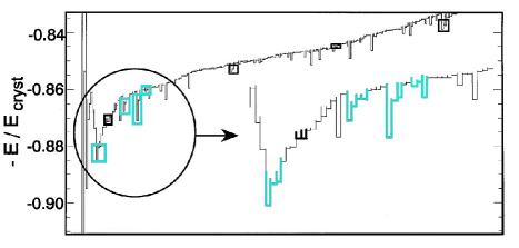
Figure 1: The PEL for a BLJ mixture of 32 particles, mapped in 1D according to the procedure by Heuer. Highlighted in black are the 2LSs, then in blue the 3LSs, 4LSs, … ensuing from multi-welled local potentials. Adapted from [29]

The second consideration is that the computer-generated PEL typically contains more complicated, local multi-welled potentials (MWPs) as well as DWPs (indeed, a representation of the PEL solely by means of DWPs and 2LSs seems rather oversimplified, though of obvious practical theoretical advantage [28]). In Fig. 1 the one-dimensional map of a molecular dynamics-generated PEL for a system of 32 particles interacting through a binary mixture Lennard-Jones potential in the glassy phase has been reproduced [29]. There are clearly DWPs, but also MWPs as we have highlighted. The tunneling Hamiltonian of a MWPs is easily written down as [11]:

$${\cal H}_{3LS}=\left(\begin{array}[]{ccc}E_{1}&D_{0}&D_{0}\cr D_{0}&E_{2}&D_{0}\cr D_{0}&D_{0}&E_{3}\end{array}\right)$$ (4)

where $E_{1},E_{2},E_{3}$ are the energy asymmetries between the wells (we have chosen the simplest case, having three wells) and $D_{0}$ is the most relevant tunneling amplitude (through saddles of the PEL, in fact). This 3LS Hamiltonian has the advantage of readily allowing for the inclusion of a magnetic field $B>0$, when coupling orbitally with a tunneling “particle” having charge $q$ ($q$ being some multiple of the electron’s charge $-e$) [11]:

$${\cal H}_{3LS}(B)=\left(\begin{array}[]{ccc}E_{1}&D_{0}e^{i\varphi/3}&D_{0}e^{-i\varphi/3}\cr D_{0}e^{-i\varphi/3}&E_{2}&D_{0}e^{i\varphi/3}\cr D_{0}e^{i\varphi/3}&D_{0}e^{-i\varphi/3}&E_{3}\end{array}\right)$$ (5)

where $\varphi/3$ is the Peierls phase for the tunneling particle through a saddle in the field, and $\varphi$ is the Aharonov-Bohm phase for a tunneling loop and is given by the usual formula:

$$\varphi=2\pi\frac{\Phi}{\Phi_{0}},\qquad\Phi_{0}=\frac{h}{|q|}$$ (6)

$\Phi_{0}$ being the appropriate flux quantum ($h$ is Planck’s constant) and $\Phi={\bf B}\cdot{\bf S}$ the magnetic flux threading the area $S$ formed by the tunneling paths of the particle in this simple model. The energy asymmetries $E_{1},E_{2},E_{3}$ typically enter through their combination $D\equiv\sqrt{E_{1}^{2}+E_{2}^{2}+E_{3}^{2}}$. One can easily convince oneself that if such a MWP is used with the standard parameter distribution, Eq. (2) with $D,D_{0}$ replacing $\Delta,\Delta_{0}$, for the description of the TS, one would then obtain essentially the same physics as for the STM 2LS-description. In other words, there is no need to complicate the minimal 2LS-description in order to study glasses at low temperatures, unless structural inhomogeneities of the RER-type and a magnetic field are present. Without the RERs, hence no distribution of the type (3), the interference from separate tunneling paths is only likely to give rise to a very weak Aharonov-Bohm effect. Hence, it will be those TSs nesting within the RERs that will give rise to an enhanced A-B effect and these TSs can be minimally described – for example – through Hamiltonian (5) and with distribution (3) thus modified to favour near-degeneracy [11]:

$${\cal P}_{3LS}^{*}(E_{1},E_{2},E_{3};D_{0})=\frac{P^{\ast}}{D_{0}(E_{1}^{2}+E_{2}^{2}+E_{3}^{2})}.$$ (7)

We remark that the incipient “crystallinity” of the RERs calls for near-degeneracy in $E_{1},E_{2},E_{3}$ simultaneously and not in a single one of them, hence the correlated form of (7). Other descriptions, with four-welled potentials or modified three-dimensional DWPs are possible for the TSs nested in the RERs and lead to the same physics as from Eqs. (5) and (7) above [30] (which describe what we call the anomalous tunneling systems, or ATSs, nesting within the RERs).

The final and most important consideration is that the TSs appear to be rather diluted defects in the glass (indeed their concentration is of the order of magnitude of that for trace paramagnetic impurities, as we shall see), hence the tunneling “particles” are embedded in a medium otherwise characterized only by simple acoustic-phonon degrees of freedom. This embedding, however, means that the rest of the material takes a part in the making of the tunneling potential for the TS’s “particle”, which itself is not moving quantum-mechanically in a vacuum. Sussmann [31] has shown that this leads to local trapping potentials that (for the case of triangular and tetrahedral perfect symmetry) must be characterized by a degenerate ground state. This means that, as a consequence of this TS embedding, our minimal model (5) must be chosen with a positive tunneling parameter [11]:

$$D_{0}>0$$ (8)

where of course perfect degeneracy is always removed by weak disorder in the asymmetries. The intrinsic near-degeneracy of (7) implies that this model should be used in its $D/D_{0}\ll 1$ limit, which in turn reduces the ATSs to effective magnetic-field dependent 2LSs and greatly simplifies the analysis together with the limit $\varphi\to 0$ which we always take for relatively weak magnetic fields. Our extended tunneling model (ETM) consists then in a collection of independent, non-interacting 2LSs described by the STM and 3LSs described by Eqs. (5) and (7) above in the said $D/D_{0}\ll 1$ and $\varphi\to 0$ limits, the 3LSs nested within the RERs and the magnetic-field insensitive 2LSs distributed in the remaining homogeneously-disordered matrix.

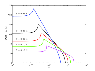
Figure 2: The magnetic-sensitive part of the density of states (DOS) as a function of the A-B phase $\varphi$ (proportional to the magnetic field $B$) and different energies ($n_{ATS}P^{\ast}$ has been set to 1). The shape of this part of the DOS (coming from the MWPs with a parameter distribution (7) favouring near-degeneracy) is the ultimate source of all the magnetic effects. The cusp is an artifact of the effective 2LS approximation [11], but also of the existence of upper and lower bounds for $D_{0}$ owing to the nature of the RER atomic structure.

Our ETM has been able to explain the magnetic effects in the heat capacity [11], in the real [32] and imaginary [33] parts of the dielectric constant and in the polarization echo amplitude [33] measurements reported to date for various glasses at low temperatures, as well as the composition-dependent anomalies [8, 34]. The new physics is provided by the magnetic-field dependent TS density of states (DOS) which acquires a term due to the near-degenerate MWPs [11] that gets added up to the (nearly) constant DOS from the STM 2LSs (having density $n_{2LS})$:

$$g_{tot}(E,B)=n_{2LS}\bar{P}+n_{ATS}\frac{P^{\ast}}{E}f_{ATS}(E,B)\theta(E-E_{c})$$ (9)

where $n_{ATS}$ is the ATSs’ concentration, $f_{ATS}$ is a magnetic-field dependent dimensionless function, already described in previous papers [11], and $E_{c}$ is a material and $B$-dependent cutoff. The $1/E$ dependence is a consequence of the chosen tunneling parameter distribution, Eq. (7) (or, to the same effect, Eq. (3)), and gives rise to a peak in $g_{tot}$ near $E_{c}$ that is rapidly eroded away as soon as a weak magnetic field is switched on. The form and evolution of the magnetic part of the DOS is shown in Fig. 2 for some typical parameters, as a function of $B$ for different values of $E$. This behaviour of the DOS with $B$ is, essentially, the underlying mechanism for all of the experimentally observed magnetic field effects in the cold glasses within this model: the measured physical properties are convolutions of this DOS (with appropriate $B$-independent functions) and in turn reproduce its shape as functions of $B$. As an example, the total TS heat capacity is given by

$$C_{pTS}(T,B)=\int_{0}^{\infty}dE~{}g_{tot}(E,B)C_{p0}(E,T)$$

where

$$C_{p0}(E,T)=k_{B}\left(\frac{E}{2k_{B}T}\right)^{2}\cosh^{-2}\left(\frac{E}{2k_{B}T}\right)$$

is the heat capacity contribution from a single TS having energy gap $E$.

We end this Section by mentioning that in model simulation studies of the 2LSs generated by defects in perfect crystals, Churkin, Barash, and Schechter [35] found non-uniform behaviour for the $g(E)$ DOS very similar to what we advocate in Eq. (9) for the ATS part (see Ref. [11], Fig. 6 for $B$=0). The (near-) crystallinity is thus the common theme between the RERs in glasses and the twin-caged defects in crystals.

A much deeper justification for our ATS model and for the nature of the TSs in general (of two types only: the 2LSs and the three- or four-fold ATSs) will be presented elsewhere, for glasses (papers in preparation).

3 Heat Capacity

3.1 Summary of previous work [11]

In this Section we re-analyze the available data [2] for the magnetic effect in the heat capacity of two multi-component glasses, commercial borosilicate Duran and barium-allumo-silicate (BAS) glass, in order to better estimate the concentration of trace Fe-impurities in this way. The presence of a magnetic effect in the Pyrex glass was reported long ago by Stephens [21] and attributed solely to paramagnetic iron impurities even though the maximum effect was for $B\simeq 0$. A systematic experimental study of $C_{p}(T,B)$ around and below 1 K in some multi-silicate glasses was carried out by Siebert [2] and those data have been used, upon permission, by one of us [11] as the very first test of the above (Section 2) ETM [11]. That earlier analysis best-fitted the $C_{p}$ data by Siebert with the sum of Einstein’s $\gamma_{ph}T^{3}$ phonon term plus the 2LS $\gamma_{2LS}T$ non-magnetic contributions, as well as with Langevin’s paramagnetic and the ATS contributions (see below). The analysis came up with concentrations $\bar{n}_{J}\simeq$48 ppm and, respectively, $\bar{n}_{J}\simeq$ 20 ppm instead of the quoted [2] 126 ppm (or 180 ppm in a different study [1]) and 102 ppm for Duran and for BAS glass, respectively.

In order to better understand this large discrepancy we begin with by re-analysing Siebert’s data for $C_{p}(T,B)$, after subtraction of the data taken at the same temperatures for the same glass, but in the presence of the strongest applied magnetic field (8 T). In this way only the magnetic-field dependent contributions should remain in the data for $\bar{C}_{p}(T,B)\equiv C_{p}(T,B)-C_{p}(T,\infty)$. It should be remarked that use of these data for $C_{p}$ is marred by the question of the many relaxation times in a glass, since the data are obtained indirectly (like in all $C_{p}$ measurements in glasses at low $T$), from a heat-pulse experiment where the change with time of the sample’s temperature is fitted with a single relaxation time involving $C_{p}$. The data thus obtained for $C_{p}$, however, strongly resemble those obtained earlier on by Stephens (at $B$=0 and 3.3 T only) [21] and there is theoretical evidence that the width of the relaxation times’ distribution narrows considerably in a magnetic field for a multi-component glass [36]. Still, we use the data of [2] tentatively.

Fig. 3 presents the data for the heat capacity after subtraction of the magnetic field independent data at $B$=8 T for the BAS glass (Fig. 3) and for Duran (Fig. 3). The parameters to be determined are the cutoff $D_{min}$ and combinations of cutoffs, charge and area $D_{0min}qS$ and $D_{0max}qS$ [11], as well as:

$n_{Fe^{2+}}$	Fe2+ impurity concentration
$n_{Fe^{3+}}$	Fe3+ impurity concentration
$n_{ATS}$	ATS concentration (always multiplied by $P^{\ast}$)

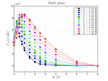
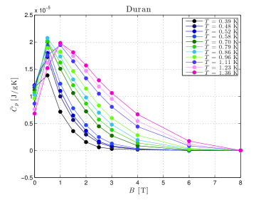
Figure 3: The heat capacity data $\bar{C}_{p}=C_{p}-C_{p}$(8 T) as a function of the magnetic field $B$ for different temperatures: a) for the BAS and b) Duran glasses. Data from [2] (also reproduced, upon permission, in [11]).

The data of Fig. 3 and Fig. 3 (we have restricted the best fit to the three temperatures having the most data points around the peak of $C_{p}(B)$) have been best-fitted by using the following magnetic-dependent contributions:

1. the known Langevin contribution of the paramagnetic Fe impurities (Fe²⁺ and Fe³⁺) having concentration $n_{J}$:

   $$C_{J}(T,B)=n_{J}\frac{k_{B}z^{2}}{4}\bigg{(}\bigg{(}\frac{1}{\sinh\frac{z}{2}}\bigg{)}^{2}-\bigg{(}\frac{2J+1}{\sinh\frac{(2J+1)z}{2}}\bigg{)}^{2}\bigg{)}$$ (10)

   where $z=\frac{g\mu_{B}JB}{k_{B}T}$ and where $g$ is Landè’s factor for the paramagnetic ion in that medium, $\mu_{B}$ is Bohr’s magneton and $J$ the ion’s total angular momentum (in units $\hbar$=1); $k_{B}$ is Boltzmann’s constant. We have assumed the same values the parameters $g$ and $J$ take for Fe²⁺ and Fe³⁺ in crystalline SiO₂: $J$=2 with $g$=2 and, respectively, $J=5/2$ with $g$=2 (we have adopted, in other words, complete quenching of the orbital angular momentum [37], consistent with other Authors’ analyses [2, 3]).

2. the averaged contribution of the ATSs [11], written in terms of a sum of individual contributions from each ATS of lowest energy gap $E$

   $$\begin{split}&C_{ATS}(T,\varphi)=\frac{\pi}{4}\frac{P^{\ast}~{}n_{ATS}}{k_{B}T^{2}}\\ &\times\Big{\{}\int_{E_{c1}}^{E_{c2}}~{}dE~{}\frac{E}{\cosh^{2}(\frac{E}{2k_{B}T})}~{}\ln\Big{[}\frac{(E^{2}-D_{0min}^{2}\varphi^{2})(E^{2}-D_{min}^{2})}{D_{min}^{2}D_{0min}^{2}\varphi^{2}}\Big{]}\\ &+\int_{E_{c2}}^{\infty}~{}dE~{}\frac{E}{\cosh^{2}(\frac{E}{2k_{B}T})}~{}\ln\Big{[}\big{(}\frac{D_{0max}}{D_{0min}}\big{)}^{2}\frac{E^{2}-D_{0min}^{2}\varphi^{2}}{E^{2}-D_{0max}^{2}\varphi^{2}}\Big{]}\Big{\}}\\ \end{split}$$ (11)

   or, re-written in a dimensionless form as

   $$\begin{split}&C_{ATS}(T,\varphi)=\widetilde{C}_{0}(T,\varphi)+2\pi P^{\ast}n_{ATS}k_{B}\Big{\{}\big{[}I(x_{c1})-I(x_{c2})\big{]}\ln(x_{min}x_{0min}\varphi)\\ &+\frac{1}{2}\big{[}\mathcal{I}(x_{c1},x_{min})-\mathcal{I}(x_{c2},x_{min})+\mathcal{I}(x_{c1},x_{0min}\varphi)-\mathcal{I}(x_{c2},x_{0max}\varphi)\Big{\}}\\ \end{split}$$ (12)

   where:

   • $E_{c1}=\sqrt{D_{min}^{2}+D_{0min}^{2}\varphi^{2}}$ and $E_{c2}=\sqrt{D_{min}^{2}+D_{0max}^{2}\varphi^{2}}$;

   • $x_{c1,2}=\frac{E_{c1,2}}{2k_{B}T}$, $x_{min}=\frac{D_{min}}{2k_{B}T}$, etc.;

   • $I(x)\equiv x\tanh x-\ln\cosh x$;

   • $\mathcal{I}(x,a)\equiv\int_{x}^{\infty}\mathrm{d}y\frac{y}{\cosh^{2}y}\ln(y^{2}-a^{2})$.

   and the following expression:

   $$\widetilde{C}_{0}(T,\varphi)=2\pi P^{\ast}n_{ATS}k_{B}\ln\bigg{(}\frac{D_{0max}}{D_{0min}}\bigg{)}\big{\{}\ln(2)-I(x_{c2}).\big{\}}\\$$ (13)

   The angular average over the ATS orientations is performed by replacing $\varphi\rightarrow\frac{\varphi}{\sqrt{3}}$ (in other words averaging $\cos^{2}\theta$, $\theta$ being the orientation of ${\bf S}$ with respect to ${\bf B}$).

3.2 Extracted parameters from best-fitting the heat capacity data

3.2.1 BAS glass

The concentrations of the ATSs and Fe-impurities extracted from the best fit of the heat capacity as a function of $B$, for the BAS glass, are reported in Table 1; having fixed the concentrations, it was possible to extract the other parameters for the BAS glass (Table 2). The best fit of the chosen data is reported in Fig. 4.

BAS glass	Concentration $\mathrm{[g^{-1}]}$	Concentration [ppm]
$n_{Fe^{2+}}$	1.06$\times 10^{17}$	14.23
$n_{Fe^{3+}}$	5.00$\times 10^{16}$	6.69
$P^{\ast}n_{ATS}$	5.19$\times 10^{16}$	-

Table 1: Extracted parameters (from the heat capacity data) for the concentrations of ATSs and Fe-impurities for the BAS glass.

Temperature [K]	$D_{min}$ [K]	$D_{0min}|\frac{q}{e}|S$ [K$\AA^{2}$]	$D_{0max}|\frac{q}{e}|S$ [K$\AA^{2}$]
0.60	0.49	4.77$\times 10^{4}$	3.09$\times 10^{5}$
0.90	0.53	5.07$\times 10^{4}$	2.90$\times 10^{5}$
1.36	0.55	5.95$\times 10^{4}$	2.61$\times 10^{5}$

Table 2: Extracted tunneling parameters (from the $C_{p}$ data) for the BAS glass.

3.2.2 Duran

The concentrations of the ATSs and Fe-impurities extracted from the best fit of the heat capacity as a function of $B$, for Duran, are reported in Table 3; having fixed the concentrations, it was possible to extract the other parameters for Duran (Table 4). The fit of the chosen data is reported in Fig. 4.

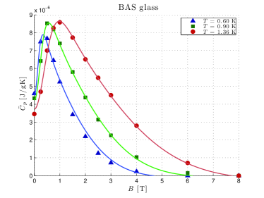
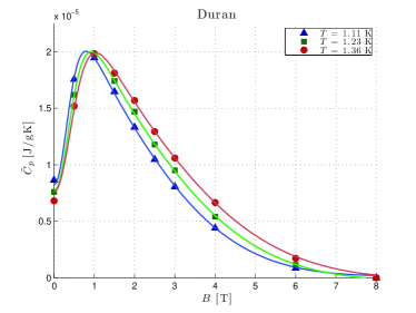
Figure 4: The heat capacity best fit for the a) BAS and b) Duran glasses.

The first comment we make is that these good fits, with a smaller set of fitting parameters, repropose concentrations and tunneling parameters very much in agreement with those previously obtained by one of us [11]. The problem with the concentrations of the Fe-impurities reported in the literature is that they do not allow for a good fit of the $\bar{C}_{p}(B)=C_{p}(B)-C_{p}(\infty)$ data in the small field region when the Langevin contribution alone is employed (Eq. (10) without Eq. (12)). See for instance Section 5, Fig. 7. The Langevin contribution drops to zero below the peak, whilst both Siebert’s and Stephens’ data definitely point to a non-zero value of $\bar{C}_{p}(0)=C_{p}(0)-C_{p}(\infty)$ at $B=0$ for any $T>0$. This non-zero difference is well accounted for by our ETM and it comes from the ATS contribution to the DOS in Eq. (9).

Duran	Concentration $\mathrm{[g^{-1}]}$	Concentration [ppm]
$n_{Fe^{2+}}$	3.21$\times 10^{17}$	33.01
$n_{Fe^{3+}}$	2.11$\times 10^{17}$	21.63
$P^{\ast}n_{ATS}$	8.88$\times 10^{16}$	-

Table 3: Extracted parameters (from the heat capacity data) for the concentration of ATSs and Fe-impurities for Duran.

Temperature [K]	$D_{min}$ [K]	$D_{0min}|\frac{q}{e}|S$ [K$\AA^{2}$]	$D_{0max}|\frac{q}{e}|S$ [K$\AA^{2}$]
1.11	0.34	4.99$\times 10^{4}$	2.68$\times 10^{5}$
1.23	0.32	5.30$\times 10^{4}$	2.50$\times 10^{5}$
1.36	0.32	5.54$\times 10^{4}$	2.46$\times 10^{5}$

Table 4: Extracted tunneling parameters (from the $C_{p}$ data) for Duran.

The results of our $C_{p}$ analysis definitely indicate that the concentration of paramagnetic impurities in the multi-silicate glasses is much lower than previously thought and extracted from SQUID-magnetometry measurements of the magnetization $M(T,B)$ at moderate to strong field values and as a function of $T$. Therefore we now turn our attention to a re-analysis of the SQUID-magnetometry data.

4 Magnetization

4.1 Theory

The second comment we make, having obtained a qualitatively (and also quantitatively, barring the multiple relaxation-times issue) good fit to the $C_{p}(B)$ data with the ATS contribution added to the Langevin’s, is that the ATSs now appear to carry considerably high magnetic moments $\mu_{ATS}$. Estimating from the definition ($T=0$) $\mu_{ATS}=-\frac{\partial}{\partial B}\big{(}-\frac{1}{2}E\big{)}$, where $E=\sqrt{D^{2}+D_{0}^{2}\varphi^{2}}$ is the ATS lower energy gap, we get for not too small fields $B$ ($\mu_{ATS}$ vanishes linearly with $B$ when $B\to 0$, but saturates at high enough $B$):

$$\mu_{ATS}\simeq\frac{\pi}{\Phi_{0}}SD_{0}=\frac{\pi}{\phi_{0}}\left(\big{|}\frac{q}{e}\big{|}SD_{0}\right).$$ (14)

Thus the very same combination $\frac{q}{e}SD_{0}$ of parameters appears, whilst $\phi_{0}\equiv h/e$ is the electronic magnetic flux quantum. Using the values extracted from the $C_{p}$ best fit (e.g. Table 4) we deduce from Eq. (14) that (for Duran) $\mu_{ATS}$ ranges from about 3.8$\mu_{B}$ to 27.1$\mu_{B}$. This fact alone indicates that a large group of correlated charged atomic particles is involved in each single ATS and that an important ATS contribution to the sample’s magnetization is to be expected (Fe²⁺ and Fe³⁺ have magnetic moment $\mu_{J}=4\mu_{B}$ and, respectively, $5\mu_{B}$).

The magnetization $M$ of a sample containing dilute paramagnetic impurities as well as dilute magnetic-field sensitive ATSs is, like $C_{p}$, also given by the sum of two different contributions:

1. Langevin’s well-known paramagnetic impurities’ contribution (Fe²⁺ and Fe³⁺, with $n_{J}$ concentration of one species having spin $J$), given by the standard expression [38]

   $$M_{J}=n_{J}g\mu_{B}JB_{J}(z),~{}~{}~{}\bigg{(}z=\frac{g\mu_{B}BJ}{k_{B}T}\bigg{)}$$ (15)

   where the Brillouin function $B_{J}$ is defined by:

   $$B_{J}(z)=\frac{2J+1}{2J}\coth\bigg{(}\frac{(2J+1)}{2J}z\bigg{)}-\frac{1}{2J}\coth\bigg{(}\frac{1}{2J}z\bigg{)}$$ (16)

   and its low-field susceptibility is the known Curie law:

   $$\frac{M}{B}\cong\frac{n_{J}g^{2}\mu_{B}^{2}J(J+1)}{3k_{B}T}$$ (17)

2. the ATS tunneling currents’ contribution, given by the following novel expression as the sum of contributions from ATSs of lowest gap $E$:

   $$\begin{split}M_{ATS}=\pi~{}P^{\ast}n_{ATS}\frac{1}{B}\bigg{\{}&\int_{E_{c1}}^{E_{c2}}\mathrm{d}E\tanh\bigg{(}\frac{E}{2k_{B}T}\bigg{)}\ln\bigg{(}\frac{E^{2}-D_{0min}^{2}\varphi^{2}}{D_{min}^{2}}\bigg{)}\\ +&\int_{E_{c2}}^{\infty}\mathrm{d}E\tanh\bigg{(}\frac{E}{2k_{B}T}\bigg{)}\ln\bigg{(}\frac{E^{2}-D_{0min}^{2}\varphi^{2}}{E^{2}-D_{0max}^{2}\varphi^{2}}\bigg{)}\bigg{\}}\end{split}$$ (18)

   and which can be also re-expressed (like in the case of $C_{ATS}$) using $y=\frac{E}{2k_{B}T}$ in the following form:

   $$\begin{split}M_{ATS}=2\pi~{}P^{\ast}n_{ATS}k_{B}T\frac{1}{B}\bigg{\{}&\int_{x_{c1}}^{x_{c2}}\mathrm{d}y\tanh y\ln\bigg{(}\frac{y^{2}-x_{0min}^{2}\varphi^{2}}{x_{min}^{2}}\bigg{)}\\ +&\int_{x_{c2}}^{\infty}\mathrm{d}y\tanh y\ln\bigg{(}\frac{y^{2}-x_{0min}^{2}\varphi^{2}}{y^{2}-x_{0max}^{2}\varphi^{2}}\bigg{)}\bigg{\}}\end{split}$$ (19)

   with, as before:

   • $E_{c1}=\sqrt{D_{min}^{2}+D_{0min}^{2}\varphi^{2}}$ and $E_{c2}=\sqrt{D_{min}^{2}+D_{0max}^{2}\varphi^{2}}$;

   • $x_{c1,2}=\frac{E_{c1,2}}{2k_{B}T}$, $x_{min}=\frac{D_{min}}{2k_{B}T}$, etc.;

We present this expression here for the first time, also motivated by the fact that we expect a contribution to the measured magnetization $M$ from the ATSs that is comparable to, or even greater than, Langevin’s paramagnetism of the diluted Fe impurities. The above expression follows from a straightforward application of standard quantum statistical mechanics, with

$${\bf M}_{ATS}=n_{ATS}\langle-\frac{\partial{\cal H}_{3LS}}{\partial{\bf B}}\rangle,$$

$n_{ATS}$ being the ATSs’ concentration (a parameter always lumped together with $P^{\ast}$) and with ${\cal H}_{3LS}$ given by Eq. (5). The angular brackets $\langle\cdots\rangle$ denote quantum, statistical and disorder averaging.

The above formula for $M_{ATS}$ is in fact correct for weak magnetic fields. For higher fields a correction has to be introduced, owing to the fact that an improved analytic expression [39] for the lowest ATS energy gap must be used:

$$E=\sqrt{D^{2}+D_{0}^{2}\varphi^{2}(1-\frac{1}{27}\varphi^{2})}.$$

A full derivation and the study of the $B$- and $T$-dependence of $M_{ATS}$ will be presented elsewhere.

4.2 Extracted parameters for the magnetization data

4.2.1 BAS glass

The magnetization data [2] were best-fitted with Eq. (15) (for the Fe²⁺ and Fe³⁺ contributions) as well as with Eq. (19) (for the ATSs’), using the parameters from the $C_{p}$-fits as input. The best fit for the BAS glass is reported in Fig. 5 and the extracted parameters in Table 5.

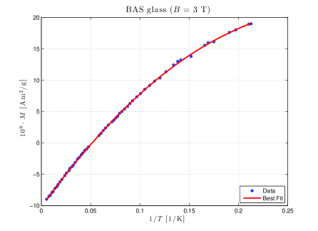
Figure 5: The best fit of the magnetization data [2] for the BAS glass, using Eq. (15) (for the Fe²⁺ and Fe³⁺ impurities) and Eq. (19) (for the ATSs).

Parameter	BAS glass
$n_{Fe^{2+}}$ $\mathrm{[g^{-1}]}$	1.08$\times 10^{17}$
$n_{Fe^{3+}}$ $\mathrm{[g^{-1}]}$	5.01$\times 10^{16}$
$P^{\ast}n_{ATS}$ $\mathrm{[g^{-1}]}$	5.74$\times 10^{16}$
$D_{min}$ [K]	8.01$\times 10^{-2}$
$D_{0min}|\frac{q}{e}|S$ [K$\AA^{2}$]	1.31$\times 10^{5}$
$D_{0max}|\frac{q}{e}|S$ [K$\AA^{2}$]	2.44$\times 10^{5}$
$\mathrm{vert.offset}$ [Am2g-1]	-1.04$\times 10^{-5}$

Table 5: Extracted parameters (from the magnetization data of [2]) for the concentration of ATS and Fe-impurities of the BAS glass. The vertical offset represents the residual Larmor diamagnetic contribution.

4.2.2 Duran

The best fit for Duran is reported in Fig. 6 and the extracted parameters in Table 6.

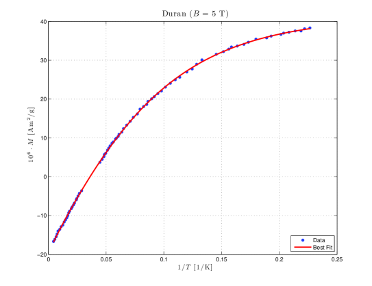
Figure 6: The best fit of the magnetization data [2] of Duran, using Eq. (15) (for the Fe²⁺ and Fe³⁺ impurities) and Eq. (19) (for the ATSs).

Parameter	Duran
$n_{Fe^{2+}}$ $\mathrm{[g^{-1}]}$	3.07$\times 10^{17}$
$n_{Fe^{3+}}$ $\mathrm{[g^{-1}]}$	2.13$\times 10^{17}$
$P^{\ast}n_{ATS}$ $\mathrm{[g^{-1}]}$	8.68$\times 10^{16}$
$D_{min}$ [K]	5.35$\times 10^{-2}$
$D_{0min}|\frac{q}{e}|S$ [K$\AA^{2}$]	2.00 $\times 10^{5}$
$D_{0max}|\frac{q}{e}|S$ [K$\AA^{2}$]	2.81$\times 10^{5}$
$\mathrm{vert.offset}$ [Am2g-1]	-1.97$\times 10^{-5}$

Table 6: Extracted parameters (from the magnetization data of [2]) for the concentration of ATS and Fe impurities of Duran.

4.3 Concentration conversion

We now explain how we convert the Fe-concentrations thus obtained to atomic ppm concentrations (ppma). $n_{J}$, the mass density of a Fe species with spin $J$ in the sample, is given by:

$$n_{J}=\frac{N_{J}}{M}=\frac{N_{J}}{N_{at}}\frac{N_{A}}{\sum_{i}\xi_{i}A_{i}}$$ (20)

where

$$M=\sum_{i}\xi_{i}\frac{N_{at}}{N_{A}}A_{i}$$ (21)

is the sample’s mass, and where:

$N_{J}$	number of Fe-ions in the sample with spin $J$
$\xi_{i}$	molar fraction of the i-$th$ species
$A_{i}$	molar mass of the i-$th$ species
$N_{at}$	total number of atoms in the sample
$N_{A}$	Avogadro’s number (6.022$\times$1023 mol-1)

for the Fe²⁺ ($J$=2) and Fe³⁺ ($J$=5/2) impurities. Table 7 shows parameters related to the chemical and molar composition [2] of the two multi-component silicate glasses. Therefore, using the parameters reported in Table 7, one has:

$$\sum_{i}\xi_{i}A_{i}=\left\{\begin{array}[]{ll}80.530\mathrm{\frac{g}{mol}}&\mathrm{for~{}BAS~{}glass}\\ 61.873\mathrm{\frac{g}{mol}}&\mathrm{for~{}Duran}\\ \end{array}\right.$$

Oxide Element	Molar Mass ($A_{i}$)	$\xi_{i,\%}$ BAS glass	$\xi_{i,\%}$ Duran
SiO2	60.084	72.7	83.4
B2O3	69.620	0.72	11.6
Al2O3	101.961	8.8	1.14
Na2O	61.979	0.28	3.4
K2O	94.196	0.064	0.41
BaO	153.326	17.0	0.005
Li2O	29.881	0.014	0.004
PbO	223.199	0.48	$<$0.01

Table 7: Molar mass $A_{i}$ and percentage fraction $\xi_{i,\%}$ of the various oxides making up the BAS (third column) and Duran (fourth column) glasses, as reported in [2, 3].

We interpret $N_{J}/N_{at}\equiv\bar{n}_{J}$ as the atomic concentration of the spin-$J$ Fe species (to be multiplied by 10⁶ to obtain the ppm) and thus we have the conversion formula:

$$n_{J}=\bar{n}_{J}\frac{N_{A}}{\sum_{i}\xi_{i}A_{i}}$$ (22)

5 Conclusions: Extracted Concentrations for Iron Impurities and ATSs

5.1 BAS glass

The nominal concentration of Fe³⁺ for the BAS glass is (using Eq. (20) or (22)):

$$\begin{split}\bar{n}_{Fe^{3+}_{nom}}&=102~{}\mathrm{ppm}\\ n_{Fe^{3+}_{nom}}&=\frac{10^{-6}\cdot 102\cdot 6.022\times 10^{23}~{}\mathrm{mol}^{-1}}{80.530\mathrm{\frac{g}{mol}}}=7.63\cdot 10^{17}\mathrm{g^{-1}}\\ \end{split}$$ (23)

which is inadequate (as in Duran’s case below) to explain the behaviour of the heat capacity as a function of $B$, here presented (Fig. 4) and as a function of $T$ (studied in [11]). Table 8 summarizes the concentrations found from our best fits of heat capacity and magnetization data, for the BAS glass. The parameters found in [11] were $P^{\ast}n_{ATS}$=6.39$\times 10^{16}$ g^-1 and $\bar{n}_{Fe}$=20.44 ppm where this latter was for the Fe²⁺ concentration only. The present study confirms that most of the Fe-impurities in these two glasses are of the Fe²⁺ type [11].

BAS glass
Heat Capacity fit
$n_{Fe^{2+}}$	1.06$\times 10^{17}~{}\mathrm{g^{-1}}$ = 14.23 ppm
$n_{Fe^{3+}}$	5.00$\times 10^{16}~{}\mathrm{g^{-1}}$ = 6.69 ppm
$P^{\ast}n_{ATS}$	5.19$\times 10^{16}~{}\mathrm{g^{-1}}$
Magnetization fit
$n_{Fe^{2+}}$	1.08$\times 10^{17}~{}\mathrm{g^{-1}}$ = 14.38 ppm
$n_{Fe^{3+}}$	5.01$\times 10^{16}~{}\mathrm{g^{-1}}$ = 6.70 ppm
$P^{\ast}n_{ATS}$	5.74$\times 10^{16}~{}\mathrm{g^{-1}}$

Table 8: Comparison between the concentrations extracted from the two different best-fitted experimental data sets for the BAS glass.

5.2 Duran

The nominal concentration of Fe³⁺ for Duran is (using Eq. (20) or (22)):

$$\begin{split}\bar{n}_{Fe^{3+}_{nom}}&=126~{}\mathrm{ppm}\\ n_{Fe^{3+}_{nom}}&=\frac{10^{-6}\cdot 126\cdot 6.022\times 10^{23}~{}\mathrm{mol}^{-1}}{61.873\mathrm{\frac{g}{mol}}}=1.23\cdot 10^{18}\mathrm{g^{-1}}\\ \end{split}$$ (24)

which again is inadequate to explain the behaviour of the heat capacity as a function of $B$ (see Fig. 7). Table 9 summarizes the concentrations found from our best fits of heat capacity and magnetization data, for Duran. The parameters found in [11] were $P^{\ast}n_{ATS}$=6.92$\times 10^{16}$ g^-1 and $\bar{n}_{Fe}$=47.62 ppm where this latter was the Fe²⁺ concentration only.

Fig. 7 presents the behaviour of the different contributions to the heat capacity as a function of $B$ for Duran; $C_{Fe^{2+}}$ and $C_{Fe^{3+}}$ are given by Eq. (10), respectively with the Fe²⁺ and Fe³⁺ parameters, $C_{param}$ is the sum of these latter two, C_ATS is given by Eq. (12) and the green line represents the result of the best fit. The dashed line corresponds to the $\bar{C}_{p}(B)$ one would get from the nominal concentration $\bar{n}_{Fe}$ of 126 ppm [2] as extracted from the SQUID magnetization measurements fitted with the Langevin contribution only (no ATS contribution). Likewise Fig. 8 presents the behaviour of the different contributions (Eq.(15) and Eq.(19)) to the magnetization as a function of $B$, also for Duran. It can be seen that the ATS contribution is in both cases dominant, also (in the case of the magnetization) at the higher temperatures.

Duran
Heat Capacity fit
$n_{Fe^{2+}}$	3.21$\times 10^{17}~{}\mathrm{g^{-1}}$ = 33.01 ppm
$n_{Fe^{3+}}$	2.11$\times 10^{17}~{}\mathrm{g^{-1}}$ = 21.63 ppm
$P^{\ast}n_{ATS}$	8.88$\times 10^{16}~{}\mathrm{g^{-1}}$
Magnetization fit
$n_{Fe^{2+}}$	3.07$\times 10^{17}~{}\mathrm{g^{-1}}$ = 31.58 ppm
$n_{Fe^{3+}}$	2.13$\times 10^{17}~{}\mathrm{g^{-1}}$ = 21.86 ppm
$P^{\ast}n_{ATS}$	8.68$\times 10^{16}~{}\mathrm{g^{-1}}$

Table 9: Comparison between the concentrations extracted from the two different best-fitted experimental data sets for Duran.

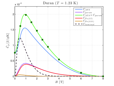
Figure 7: The curves represent the different terms that contribute to the heat capacity of Duran in our best fit of the data from [2]. The dashed curve is for Langevin’s contribution only, but with the nominal concentration of $\bar{n}_{Fe^{3+}}$=126 ppm (no ATS).

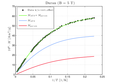
Figure 8: The curves represent the different contributions to the magnetization of Duran in our best fit of the data from [2].

5.3 Conclusions and outlook

In conclusion, by allowing a contribution to the magnetization from the ATS tunneling currents as evaluated from our ETM we have been able to show that the concentrations of Fe impurities (of type Fe²⁺ as well as Fe³⁺) are in much better agreement when extracted from SQUID magnetization data or from heat capacity data with the samples in a magnetic field. We have aimed at a semi-quantitative agreement, but inclusion of a possible contribution to $C_{p}$ from Kramers-doublets’ splitting for the $J=5/2$ Fe³⁺ species [2] (which we confirm, however, to be the minority one [11]) could possibly further improve the quantitative agreement.

We reach the surprising conclusion that the ATSs and the ETM employed keep giving a good description of the glass magnetization till the highest temperatures in the SQUID-magnetometry measurements, about 300 K (the glass-transition temperature $T_{g}$ being, however, 1123 K for BAS glass and 803 K for Duran, respectively [2]). This new finding is interpreted with the consideration that no phonon-TS interactions are involved in the measurement of the magnetization, contrary to the case of AC dielectric-constants and polarization-echo measurements, or to the case of the acoustic measurements, or that of the heat capacity, where phonons do contribute and in a complicated way well above 1 K [4, 6]. The SQUID magnetization measurement in a magnetic field is thus an ideal arena where to study the TSs in general and to test our ETM, proposed for the explanation of the magnetic effects in the multi-component glasses as manifestations of the inhomogeneous structure of the glassy state. Therefore a systematic experimental study of SQUID magnetization as a function of $T$ and $B$ from multi-component glasses with very low paramagnetic impurity concentration (e.g. BK7) would be most welcome to test our model. Moreover, also the tunneling parameters and the concentration of the ATSs here obtained turn out to be similar when extracted from the $C_{p}$- and from the $M$-data, with the tunneling parameters $D_{min}$, $D_{0min}|\frac{q}{e}|S$ and $D_{0max}|\frac{q}{e}|S$ extracted from the $M$-data being as anomalously large as from best-fits of all data in the other experiments [11, 32, 33, 34]. These large values have been interpreted by one of us [8] as deriving from the correlated tunneling of a large, but not yet mesoscopic or macroscopic, number $N\sim$ 200 to 600 of atomic-scale TSs, the ATS being only a fictitious tunneling particle involving in fact the correlated rearrangement of a large group of (charged) atoms. There appears to be a weak temperature dependence $N(T)$ of this number of correlated atomic tunnelers, since the parameters quoted above change slightly (or even significantly, yet remaining large) from experiment to experiment carried out at different temperature ranges. About this revealing $T$-dependence will be expanded in future publications.

We remark that the concentration $n_{J}$ of paramagnetic impurities turns out to be significantly lower, up to 80% less, than the concentrations reported in the literature for the analysed glasses and as extracted from SQUID-measurements of the magnetization [1, 2, 9]. Our point of view is that without the inclusion of the contribution from the ATSs the extracted SQUID-measurement concentration of paramagnetic impurities will be considerably overestimated. This happened already in the case of Stephens’ data [21], which have led to the Langevin-only estimate [11] $\bar{n}_{Fe}\simeq$ 50 ppm in Pyrex from the $C_{p}$ measurement data in a magnetic field, when in fact the mass-spectrometry analysis had given [21] $\bar{n}_{Fe}$=12 ppm. The fact that we have established, that Langevin-only fitted SQUID-magnetization measurements considerably overestimate the concentration of paramagnetic impurities in a glassy matrix, would appear to cast serious doubts about the trace Fe-impurities and associated paramagnetic-TSs as possible sources of the magnetic effects in the cold glasses [12]. Indeed, Fe³⁺ would enter substitutionally to Si⁴⁺ only in a crystal (e.g. quartz), whilst in a multi-silicate glass the overwhelming majority of Fe-impurities would enter as network-modifiers of the SiO₄ glassy matrix [40]. This means that the amplitude of the [FeO₄]^- paramagnetic-TS contribution should be reduced considerably more than the 80% we claim from the overestimate of the Fe-concentration from Langevin-fitted SQUID-measurements. We note in passing that the paramagnetic-TS explanation of the magnetic effect in $C_{p}$ requires concentrations $n_{Fe}$ already some 40% greater than the nominal, Langevin-only SQUID-extracted values [12]. The paramagnetic-TS approach may nevertheless retain some validity in the case of the heavily Fe- and Cr-doped multi-silicate glasses [41].

Appendix

Here we present our preliminary study of the SQUID magnetization data (also available from [2]) for the borosilicate glass BK7, for which however no substantial magnetic effect in the heat capacity $C_{p}$ has been reported [2]. This glass has a nominal Fe-impurity concentration of $\bar{n}_{Fe^{3+}}$=6 ppm [2, 3, 9], yet our best fit in Fig. A1 with both Langevin (Eq. (15)) and ATS (Eq. (19)) contributions produces the concentrations and parameters given in Table A1. The best fit was carried out with knowledge of ATS parameters from our own theory [33] for the magnetic effect in the polarization-echo experiments at mK temperatures [3]. We conclude that our main contention is once more confirmed, in that the concentration of Fe in BK7 we extract in this way is only about 1.1 ppm and the bulk of the SQUID magnetization is due to the ATSs. Table A1 reports our very first estimate of $n_{ATS}P^{\ast}$ for BK7. Assuming $P^{\ast}$ to be of order 1 and about the same for all glasses, we conclude that the concentration $n_{ATS}$ of the ATSs nesting in the RERs is very similar for all of the multi-silicate glasses by us studied for their remarkable magnetic effects. From the present SQUID-magnetization best fits we have obtained 5.74$\times 10^{16}$ g^-1 (BAS glass), 8.68$\times 10^{16}$ g^-1 (Duran) and 1.40$\times 10^{16}$ g^-1 (BK7). The almost negligible magnetic effect in $C_{p}$ for BK7 is due, in our approach, to the low values of the cutoffs $D_{0min}$ and $D_{0max}$ for this system (these parameters appearing in the prefactor and in the integrals’ bounds determining the ATS contribution to $C_{p}$ [8]).

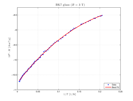
Figure A1: The best fit of the magnetization data [2] for BK7, using Eq. (15) (for the Fe²⁺ and Fe³⁺ impurities) and Eq. (19) (for the ATSs). Data from [2].

Parameter	BK7
$n_{Fe^{2+}}$ $\mathrm{[g^{-1}]}$	6.69$\times 10^{15}$ = 0,71 ppm
$n_{Fe^{3+}}$ $\mathrm{[g^{-1}]}$	3.43$\times 10^{15}$ = 0.36 ppm
$P^{\ast}n_{ATS}$ $\mathrm{[g^{-1}]}$	1.40$\times 10^{16}$
$D_{min}$ [K]	5.99$\times 10^{-2}$
$D_{0min}|\frac{q}{e}|S$ [K$\AA^{2}$]	8.87$\times 10^{4}$
$D_{0max}|\frac{q}{e}|S$ [K$\AA^{2}$]	1.20$\times 10^{5}$
$\mathrm{vert.offset}$ [Am2g-1]	-1.08$\times 10^{-5}$

Table A1: Extracted parameters (from the magnetization data of [2]) for the concentration of ATSs and Fe impurities of the BK7 ($\sum_{i}\xi_{i}A_{i}$= 63.530 g mol^-1 [2]). The vertical offset represents the residual Larmor diamagnetic contribution.

References

- [*] email: giancarlo.jug@uninsubria.it (corresponding author)
- [1] T. Herrmannsdörfer and R. König: Magnetic Impurities in Glass and Silver Powder at Milli- and Microkelvin Temperatures, J. Low Temp. Phys. 118(1-2): 45–57 (2000).
- [2] L. Siebert: Ph.D. Thesis Heidelberg University (2001), www.ub.uni-heidelberg.de/archiv/1601
- [3] S. Ludwig, P. Nagel, S. Hunklinger and C. Enss: Magnetic Field Dependent Coherent Polarization Echoes in Glasses, J. Low Temp. Phys. 131(1-2): 89–111 (2003).
- [4] P. Esquinazi (Ed.): Tunneling Systems in Amorphous and Crystalline Solids (Springer, Berlin, 1998).
- [5] G. Schuster, G. Hechtfischer, D. Buck and W. Hoffmann: Thermometry below 1 K, Rep. Prog. Phys. 57(2), 187–230 (1994).
- [6] W.A. Phillips: Two-level States in Glasses, Rep. Prog. Phys. 50(12): 1657–1708 (1987).
- [7] H.M. Carruzzo, E.R. Grannan, and C.C. Yu: Nonequilibrium Dielectric Behavior in Glasses at low Temperatures: Evidence for Interacting Defects, Phys. Rev. B 50(10), 6685–6695 (1994).
- [8] G. Jug and M. Paliienko: Multilevel Tunneling Systems and Fractal Clusters in the Low-Temperature Mixed Alkali-Silicate Glasses, Sci. World J. 2013, 1–20 (2013).
- [9] M. Wohlfahrt, P. Strehlow, C. Enss, and S. Hunklinger: Magnetic-Field Effects in non-magnetic Glasses, Europhys. Lett. 56, 690–694 (2001).
- [10] A. Würger, A Fleischmann and C. Enss: Dephasing of Atomic Tunneling by Nuclear Quadrupoles Phys. Rev. Lett. 89(23), 37601 (2002).
- [11] G. Jug: Theory of the Thermal Magnetocapacitance of Multi-component Silicate Glasses at Low Temperature, Phil. Mag. 84(33), 3599–3615 (2004).
- [12] A. Borisenko: Hole-compensated Fe3+ Impurities in Quarz Glasses: a Contribution to sub-Kelvin Thermodynamics, J. Phys.: Cond. Matter 19(41), 416102 (2007).
- [13] R. W. Simmonds, K. M. Lang, D. A. Hite, S. Nam, D. P. Pappas, and John M. Martinis: Decoherence in Josephson Phase Qubits from Junction Resonators, Phys. Rev. Lett. 93(7), 077003 (2004).
- [14] A. Amir, Y. Oreg and Y. Imry: On Relaxations and Aging in Various Glasses, Proc. Nat. Acad. Sci. 109(6), 1850–1855 (2012)
- [15] S. Ludwig and D. D. Osheroff: Field-Induced Structural Aging in Glasses at Ultralow Temperatures Phys. Rev. Lett. 91(10), 105501 (2003).
- [16] H. Paik and K.D. Osborn: Reducing quantum-regime Dielectric Loss of Silicon Nitride for Superconducting Quantum Circuits, Appl. Phys. Lett. 96, 072505(1–3) (2010)
- [17] Xiao Liu, D.R. Queen, T.H. Metcalf, J.E. Karel, and F. Hellman: Hydrogen-Free Amorphous Silicon with No Tunneling States, Phys. Rev. Lett. 113, 025503 (2014)
- [18] A. M. Zagoskin, S. Ashhab, J. R. Johansson, and F. Nori: Quantum Two-Level Systems in Josephson Junctions as Naturally Formed Qubits, Phys. Rev. Lett., 97, 077001 (2006).
- [19] E.-J. Donth, The Glass Transition (Springer, Berlin 2001)
- [20] L. Berthier and G. Biroli: Theoretical Perspective on the Glass Transition and Amorphous Materials, Rev. Mod. Phys., 83(2) 587–645
- [21] R.B. Stephens: Intrinsic Low-Temperature Thermal Properties of Glasses Phys. Rev. B 13(2), 852 (1976)
- [22] K. Vollmayr-Lee and A. Zippelius: Heterogeneities in the Glassy State, Phys. Rev. E 72(4), 041507 (2005)
- [23] L. Berthier, G. Biroli, J.-P. Bouchaud, L. Cipelletti and W. van Saarloos (Eds.): Dynamical Heterogeneities in Glasses, Colloids and Granular Media, (Oxford UP, 2011)
- [24] A.C. Wright, Crystalline-like Ordering in Melt-quenched Network Glasses? J. Non-cryst. Solids 401 4–26 (2014)
- [25] M.M.J. Treacy, K.B. Borisenko: The Local Structure of Amorphous Silicon, Science 335(6071) 950–953 (2012)
- [26] J. Hwang, Z.H. Melgarejo, Y.E. Kalay, I. Kalay, M.J. Kramer, D.S. Stone, P.M. Voyles: Nanoscale Structure and Structural Relaxation in ZrCuAl5 Bulk Metallic Glass, Phys. Rev. Lett. 108(19) 195505 (2012)
- [27] H. Bach and D. Krause: Analysis of the Composition and Structure of Glass and Glass Ceramics (Springer, New York 1999)
- [28] Yu, C. C., and A. J. Leggett: Low Temperature Properties of Amorphous Materials: Through a Glass Darkly, Comments on Condensed Matter Physics 14(4) 231–251 (1988)
- [29] A. Heuer: Properties of a Glass-Forming System as Derived from Its Potential Energy Landscape, Phys. Rev. Lett. 78(21) 4051–4054 (1997)
- [30] S. Bonfanti and G. Jug: to be published (2015)
- [31] J. A. Sussmann, Electric Dipoles due to Trapped Electrons, Proc. Phys. Soc. 79 758–774 (1962)
- [32] G. Jug: Multiple-well Tunneling Model for the Magnetic-field Effect in Ultracold Glasses Phys. Rev. B 79(18), 180201 (2009)
- [33] G. Jug, M. Paliienko and S. Bonfanti: The Glassy State — Magnetically Viewed from the Frozen End, J. Non-Crys. Solids 401 66–72 (2014)
- [34] G. Jug and M. Paliienko: Evidence for a Two-component Tunnelling Mechanism in the Multicomponent Glasses at low Temperatures, Europhys. Lett. 90 36002 (2010)
- [35] A. Churkin, D. Barash, and M. Schechter: Non-homogeneity of the Density of States of Tunneling Two-level Systems at low Energies, Phys. Rev. B 89, 104202 (2014)
- [36] G. Jug: to be published (2015)
- [37] A. Abragam and B. Bleaney The Physical Principles of Electron Paramagnetic Resonance (Clarendon, Oxford 1970)
- [38] N.W. Ashcroft and N.D. Mermin, Solid State Physics (Saunders College, Philadelphia 1976)
- [39] M. Paliienko: Multiple-welled Tunnelling Systems in Glasses at low Temperatures (Ph.D. Thesis, Università degli Studi dell’Insubria, 2011) http://insubriaspace.cineca.it/handle/10277/420
- [40] B. Henderson and G.F. Imbush, Optical Spectroscopy of Inorganic Solids (Oxford UP, NY 1989)
- [41] A. Borisenko and G. Jug, Paramagnetic Tunneling Systems and their Contribution to the Polarization Echo in Glasses, Phys. Rev. Lett. 107 075501 (2011)