Estimation of Zero Intelligence Models by L1 Data

Abstract

A unit volume zero intelligence (ZI) model is defined and the distribution of its L1 process is recursively described. Further, a generalized ZI (GZI) model allowing non-unit market orders, shifts of quotes and general in-spread events is proposed and a formula for the conditional distribution of its quotes is given, together with a formula for price impact. For both the models, MLE estimators are formulated and shown to be consistent and asymptotically normal. Consequently, the estimators are applied to data of six US stocks from nine electronic markets. It is found that more complex variants of the models, despite being significant, do not give considerably better predictions than their simple versions with constant intensities.

Keywords: Limit Order Market, Stochastic Models, Econometric Methods,

1 Introduction

With the recent wide expansion of trading according to continuous double auction (CDA), the importance of mathematical modelling of this trading mechanism grows.

A number of models of CDA exist which assume a rational behaviour of agents involved (see, e.g., Parlour and Seppi (2008) and the references therein); these models are, however, dependent on many arbitrary assumptions and do not give much better empirical results than models assuming a purely random behaviour of agents (see Gode and Sunder (1993) for a discussion). Thus, as an alternative to the “rational” approach, zero intelligence (ZI) models of the CDA started to be studied: out of a number of similar models of that kind, let us name Stigler (1964); Maslov (2000); Challet and Stinchcombe (2001); Luckock (2003); Smith et al. (2003); Mike and Farmer (2008) or Cont et al. (2010). All these models assume unit order sizes, Poisson arrivals of market and limit orders and locally constant cancellation rates depending on the distance to the quotes. For a survey of the ZI models and their characteristics, see Chakraborti et al. (2011a) and Chakraborti et al. (2011b), especially Section II of the latter paper. For the recent developments, see Abergel et al. (2011).

Although, according to their advocates, the ZI models are able to mimic many stylised empirical facts such as fat tails or non-Gaussianity (Slanina (2001, 2008); Šmíd (2008); Cont (2011)), no rigorous statistical evidence in that respect has been presented yet due to intractability of these models. In Šmíd (2012), a conditional distribution given L1 data is described; however, the model considered in this paper is too general to ensure consistency of statistical estimators.

The present paper simplifies the approach of Šmíd (2012) by assuming only a finite number of prices so that it is possible to construct consistent asymptotically normal estimators of the models’ parameters.

The exposition is started by introducing a sufficiently general setting covering a wide range of existing zero intelligence (ZI) models, e.g., an early work of Stigler (1964), the model by Cont et al. (2010), a discretised version of Luckock (2003) and a slightly modified version of Smith et al. (2003). After demonstrating ergodicity of the covered models, a conditional density of jumps of the L1 process (i.e., the bid, the ask, and the corresponding offered volumes) given its history is formulated.

Further, in order to treat the most obvious discrepancies between the ZI models and reality, a generalised (GZI) setting is proposed, which allows shifts of the quotes, non-unit market orders and general distributions of inside-the-spread events. A formula for a conditional density of the out-of-spread jumps of the quotes, later used in estimating the in-book parameters, is given.

Subsequently, Maximum Likelihood estimators are formulated and several variants of both the ZI and GZI models are estimated by means of L1 data for six stocks on nine US electronic markets. Further, for each stock-market pair, the variants of the models are compared by their ability to forecast magnitudes of the quotes’ jumps. It is found that more complicated variants of the models do not bring significant improvements in comparison with the simple variant with constant intensities, which itself, however, nearly always performs significantly better than a naive prediction of the jumps. It is also found that GZI variants of the models do not perform significantly better than their ZI counterparts.

This paper is organised as follows: First, the ZI setting is defined (Section 2) and the distribution of the L1 process given its history is derived. Consequently, the GZI setting is introduced and a formula for the density of the out-of-spread jumps and volume changes is given (Section 3). Finally, the empirical evidence is discussed (Section 4) and the paper is concluded (Section 5). The Appendix includes a proof of Theorem 2.2 (Appendix A), a proof of asymptotic properties of the MLE estimator (Appendix B), and detailed results on the estimation (Appendix C).

2 Zero Intelligence Model

2.1 Definition

Consider a general discrete-price continuous-time zero intelligence model with unit order sizes described by a pure jump type process

$$\Xi_{t}=(A_{t},B_{t}),\qquad t\geq 0,$$

where

$$A_{t}=(A^{1}_{t},A^{2}_{t},\dots,A^{n}_{t})\in\mathbb{N}^{n}_{0},$$

and

$$B_{t}=(B^{1}_{t},B^{2}_{t},\dots,B^{n}_{t})\in\mathbb{N}^{n}_{0},$$

are the sell limit order book and buy limit order book, respectively; here, $n$ is a number of possible prices (ticks) and, for any $p$, $A^{p}_{t}$ ($B^{p}_{t}$) stands for the number of the sell (buy) limit orders with price $p$ waiting at time $t$. Further, denote by

$$a_{t}:=\inf\left\{p:\,A_{t}(p)>0\right\}\vee 0,\qquad b_{t}:=\sup\left\{p:\,B_{t}(p)>0\right\}\wedge n+1,$$

the (best) ask and bid respectively. The list of possible events causing jumps of $\Xi$ together with the notation for their intensities is given in the following table:

code - $e$	intensity - $I_{t}(e)$	description
$\mathrm{BMO}$	$\theta_{t}=\theta(a_{t},b_{t})$	An arrival of a buy market order, causing $A^{a_{t}}$ to decrease by one (if the sell limit order book is empty then the arrival of the market order has no effect).
$\mathrm{SLO}(p)$	$\kappa_{t,p}=\kappa(a_{t},b_{t},p)$	An arrival of a sell limit order with limit price $p>b_{t}$ causing an increase of $A^{p}$ by one.
$\mathrm{CA}(p)$	$\rho_{t,p}=A^{p}_{t}\rho(a_{t},b_{t},p)$	A cancellation of a pending sell limit order with a limit price $p$ causing a decrease of $A^{p}$ by one.
$\mathrm{SMO}$	$\vartheta_{t}=\vartheta(a_{t},b_{t})$	An arrival of a sell market order, causing $B^{b_{t}}$ to decrease by one (if the buy limit order book is empty then the arrival of a market order has no effect).
$\mathrm{BLO}(p)$	$\lambda_{t,p}=\lambda(a_{t},b_{t},p)$	An arrival of a buy limit order with limit price $p<a_{t}$ causing an increase of $B^{p}$ by one.
$\mathrm{CB}(p)$	$\sigma_{t,p}=B^{p}_{t}\sigma(a_{t},b_{t},p)$	A cancellation of a pending buy limit order with a limit price $p$ causing a decrease of $B^{p}$ by one.

Here, all $\theta,\kappa,\rho,\vartheta,\lambda,\sigma$ are measurable functions.

It is assumed that all the flows of the market orders, and the flows of limit orders as well as their cancellations are mutually independent in the sense that the conditional distribution of the relative time of the first event following $t\in\mathbb{R}^{+}_{0}$ given the history of $\Xi$ up to $t$ is exponential with parameter

$$\Lambda_{t}=\theta_{t}+\vartheta_{t}+\sum_{p=b_{t}+1}^{n}\kappa_{p,t}+\sum_{p=0}^{a_{t}-1}\lambda_{p,t}+\sum_{p=a_{t}}^{n}A_{t}^{p}\rho_{p,t}+\sum_{p=0}^{b_{t}}B_{t}^{p}\sigma_{p,t}$$ (1)

and that

the probability that the next event will be of type $$e I_{t}(e)/\Lambda_{t}$$ equals to (2)

where $I_{t}(e)$ is the intensity of event $e$ at $t$. It is obvious that $\Xi$ is then a Markov chain in a countable state space.

Finally, it is assumed that $a_{0},b_{0}$ are deterministic and

$$\text{$A^{a_{0}+1}_{0},A^{a_{0}+2}_{0},\dots$ are Poisson with parameters $\iota_{a_{0}+1},\iota_{a_{0}+2},\dots$,}\\ \text{mutually independent and independent of $B_{0}$}$$ (3)

where $\iota_{\bullet}\geq 0$ are constants, and that a symmetric assumption holds for $B$.

2.2 Relation to Existing Models

The following table shows how some of the models mentioned in the Introduction comply with our setting. When speaking about Luckock (2003), we have its discretised version (see Šmíd (2012), Sec 3.3) in mind. When speaking about Smith et al. (2003), we are considering its bounded version (i.e., contrary to Smith et al. (2003) we assume zero arrival intensities for prices smaller than one and greater than $n$ ).

model	$\theta$	$\vartheta$	$\kappa$	$\rho$	$\lambda$	$\sigma$
Luckock (2003)	$K(b_{t})$	$1-L(a_{t}-1)$	$\kappa^{l}_{p}$	$0$	$\lambda^{l}_{p}$	$0$
Smith et al. (2003)	$\theta^{s}$	$\theta^{s}$	$\kappa^{s}$	$\rho^{s}$	$\kappa^{s}$	$\rho^{s}$
Cont et al. (2010)	$\theta^{c}$	$\theta^{c}$	$\kappa^{c}(p-b_{t})$	$\rho^{c}(p-b_{t})$	$\kappa^{c}(a_{t}-p)$	$\rho^{c}(a_{t}-p)$

Here, $\kappa^{l}_{p}=K(p)-K(p-1)$, $\lambda^{l}_{p}=L(p)-L(p-1)$ where $K$, $L$ are (continuous) cumulative distribution functions, $\kappa^{c},\rho^{c}$ are measurable functions and the rest of the symbols are constants.

Some of the models from the Introduction were not mentioned in the table: We did not include either Maslov (2000) or Challet and Stinchcombe (2001) because they both consider discrete time and are very similar to Smith et al. (2003) with $\rho=\sigma=0$, Cont et al. (2010), respectively. The model by Mike and Farmer (2008) was not included because of its complicated cancellation sub-model and because, apart from the cancellations, it is similar to that of Cont et al. (2010). Finally, we did not include Stigler (1964) because it is a special version of Luckock (2003) (with $K(x)=L(x)=x$).

2.3 Distribution

Let us start with a result which will guarantee that sampling from the model will give enough information to a statistician.

Proposition 2.1.

If $\rho(\bullet)>0$, $\sigma(\bullet)>0$, $\theta(\bullet)>0$ and $\vartheta(\bullet)>0$. then $\Xi_{t}$ is ergodic.

Proof.

The Proposition may be proved analogously to Cont et al. (2010), Proposition 2, where the ergodicity is verified by finding a Markov chain in $\mathbb{N}_{0}$ dominating the total number of orders with a recurrent zero state. In particular, it suffices to replace the definition of $\lambda$ and $\mu_{i}$ from Cont et al. (2010) by

$$\lambda=\sum_{p=1}^{n}[\max_{a,b,p}\kappa(a,b,p)+\max_{a,b,p}\lambda(a,b,p)],$$

and

$$\mu_{i}=\min_{a,b}\theta(a,b)+\min_{a,b}\vartheta(a,b)+i\min_{a,b,p}[\min(\rho(a,b,p),\sigma(a,b,p)].$$

∎

Our next goal is to derive a recursive analytic expression of the distribution of

$$x_{\tau}=(a_{\tau},b_{\tau},q_{\tau},r_{\tau})_{\tau\geq 0},\qquad q_{\tau}=A^{a_{\tau}}_{\tau},\quad r_{\tau}=B^{b_{\tau}}_{\tau},\quad\tau\geq 0$$

(the L1 process). To do so, let us denote by $t_{1},t_{2},\dots$ the jumps of $x$ and, in order to avoid frequent double indexing, let us write $y_{[i]}$ instead of $y_{t_{i}}$ and $y_{[i-]}$ instead of $y_{t_{i}-}$ for any process $y$. For each $i$, we want to evaluate

$$\mathbb{P}[(\Delta t_{i},x_{[i]})\in\bullet|\xi_{[i-1]}],\qquad\xi_{[k]}=(x_{[k]},\Delta t_{k},x_{[k-1]},\dots,x_{0}),\quad k\geq 0,$$

starting with

$$\mathbb{P}[(\Delta t_{i},a_{[i]},q_{[i]})\in\bullet|\xi_{[i-1]}].$$

To this end, note that

• $a$ jumps down if and only if a limit order arrives into the spread, in which case a limit price of the new order becomes a new value of $a$.

• $a$ jumps up if and only if the offered volume of the ask decreases to zero due to either a market order arrival or a cancellation, in which case the closest occupied tick becomes a new value of $a$.

Formally,

$$(a_{[i]},q_{[i]})=\begin{cases}(b_{[i-1]}+1,1)&e_{i}=\mathrm{SLO}(b_{[i-1]}+1)\\ (b_{[i-1]}+2,1)&e_{i}=\mathrm{SLO}(b_{[i-1]}+2)\\ \dots&\\ (a_{[i-1]}-1,1)&e_{i}=\mathrm{SLO}(a_{[i-1]}-1)\\ (a_{[i-1]},q_{[i-1]}+1)&e_{i}=\mathrm{SLO}(a_{[i-1]})\\ (a_{[i-1]},q_{[i-1]}-1)&e_{i}\in\{\mathrm{BMO},\mathrm{CA}(a_{[i-1]})\},q_{[i-1]}>1\\ (d_{i},A^{d_{i}}_{[i-]})&e_{i}\in\{\mathrm{BMO},\mathrm{CA}(a_{[i-1]})\},q_{[i-1]}=1\\ (a_{[i-1]},q_{[i-1]})&\text{otherwise}\end{cases}$$ (4)

$$d_{i}=\inf\{\pi:\pi>a_{[i-1]},A^{\pi}_{[i-]}>0\}\wedge n+1$$

where $e_{i}$ is the type of an event happening at $t_{i}$ and where $A^{n+1}\equiv 0$ by definition. Thus, to determine the conditional distribution of $(\Delta t_{i},a_{[i]},q_{[i]})$, it suffices to know a joint distribution of $(\Delta t_{i},e_{i},A_{[i-]})$ which is described by the following Theorem in three steps:

Theorem 2.2.

(i) For any $\tau$ and $e$,

$$\mathbb{P}[\Delta t_{i}>\tau,e_{i}=e|\xi_{[i-1]}]=\exp\{-\gamma_{i-1}\tau\}\pi_{i}(e),$$

where

$$\pi_{i}(e)=\gamma^{-1}_{i-1}\times\begin{cases}\kappa_{p,[i-1]},&e=\mathrm{SLO}(p),b_{[i-1]}<p\leq a_{[i-1]},\\ \theta_{[i-1]},&e=\mathrm{BMO},\\ \rho_{[i-1]},&e=\mathrm{CA}(a_{[i-1]}),\\ \lambda_{p,[i-1]},&e=\mathrm{BLO}(p),b_{[i-1]}\leq p<a_{[i-1]},\\ \vartheta_{[i-1]},&e=\mathrm{SMO},\\ \sigma_{[i-1]}&e=\mathrm{CB}(b_{[i-1]}),\end{cases}$$

and, for any $k$,

$$\gamma_{k}=\theta_{[k]}+\vartheta_{[k]}+\rho_{[k]}+\sigma_{[k]}+\sum_{p=b_{[k]}+1}^{a_{[k]}}\kappa_{p,[k]}+\sum_{p=b_{[k]}}^{a_{[k]}-1}\lambda_{p,[k]}.$$

(ii) Denote by $\mathrm{\boldsymbol{\delta}}_{c}$ the Dirac measure concentrated in $c$ (i.e., the distribution of constant $c$) and write $\circ$ for convolution (i.e., summation of two independent variables). For any $i$ and $p$,

$$A^{p}_{[i-]}|\xi_{[i-]}\sim\begin{cases}0&\text{on $[1\leq p<a_{[i-1]}]$}\\ \mathrm{\boldsymbol{\delta}}_{q_{[i-1]}}&\text{on $[p=a_{[i-1]}]$}\\ \mathrm{Bi}\left(\nu_{p,i},\varpi_{p,i}\right)\circ\mathrm{Po}\left(\epsilon_{p,i}+\iota_{p,i}\right)&\text{on $[a_{[i-1]}<p\leq n]$}\end{cases}$$

where

$$\xi_{[i-]}=(e_{i},\Delta t_{i},\xi_{[i-1]}),\qquad\nu_{p,i}=\begin{cases}A^{p}_{[k_{i}(p)-]}&k_{i}(p)>0,\\ 0&k_{i}(p)=0,\end{cases}\qquad\varpi_{p,i}=\begin{cases}\prod_{j=k_{i}(p)}^{i-1}\delta_{p,j}&k_{i}(p)<i\\ 1&k_{i}(p)=i\end{cases}$$

$$\epsilon_{p,i}=\sum_{j=k_{i}(p)}^{i-1}\phi_{p,j}(1-\delta_{p,j})\prod_{m=j+1}^{i-1}\delta_{p,m},\qquad\iota_{p,i}=\begin{cases}0&k_{i}(p)>0,\\ \iota_{p}\prod_{j=0}^{i-1}\delta_{p,j}&k_{i}(p)=0,\end{cases}$$

$$k_{i}(p)=\min\{k\geq 0,a_{[k]}<p\}\vee i$$

and, for any $k$,

$$\phi_{p,k}=\frac{\kappa_{p,[k]}}{\rho_{p,[k]}},\qquad\delta_{p,k}=\exp\{-\rho_{p,[k]}\Delta t_{k+1}\}$$

(iii) $A^{1}_{[i-]},A_{[i-]}^{2},\dots,A_{[i-]}^{n}$ are mutually conditionally independent given $\xi_{[i-]}$.

Proof.

See Appendix A. ∎

Before proceeding further, let us illustrate point (ii) of the Theorem, which is somewhat opaque, by an example.

Exapmle 2.3.

Consider model by Smith et al. (2003) with $\iota_{\bullet}\equiv 0$ (implying $\iota_{\bullet,3}\equiv 0$). Let $i=3$, $a_{0}=2$, $q_{0}=1$, $a_{[1]}=3$, $q_{[1]}=2$, $a_{[2]}=1$, $q_{[2]}=3$ (see Figure 1 for an illustration).

Let us start with $p=2$: as no orders could be present in tick $2$ before $t_{2}$ (the ask was above 2 that time), all the in-book orders present in the tick $t_{3}$ are those having arrived between $t_{2}$ and $t_{3}$ and not being cancelled. According to Appendix A, number of those orders is $\mathrm{Po}(\epsilon_{i,3})$ (to check it, note that $k_{i}(3)=2$ so $\nu_{i,2}=A^{2}_{[2-]}=0$ and $\epsilon_{i,3}=\frac{\kappa}{\rho}[1-\exp\{-\rho\Delta t_{3}\}]$ which, according to Appendix A, is actually the distribution of the immigration and death process of length $\Delta t_{3}$).

For $p=3$, the situation is the same with the difference that number of initial orders having survived until $t_{3}$, which is distributed according to $\mathrm{Bi}(2,\exp\{-\rho\Delta t_{3}\})=\mathrm{Bi}(A^{3}_{[3-]},\delta_{i,3})$, has to be added to $A^{p}_{[i-]}$.

Further, as the orders present in tick 4 at $t_{3}$ are exactly those having arrived from the start and not being cancelled, $A^{4}_{[i-]}|\xi_{[i-]}\sim\mathrm{Po}\left(\frac{\kappa}{\rho}[1-\exp\{-\rho t_{3}\}\right)$ - it is easy to check that (ii) gives the same result.

Finally, because $k_{i}(1)=3$, we have $\epsilon_{1,i}=0$, $\omega_{1,i}=1$ and $\nu_{1,i}=3$ so, according to (ii), $A^{1}_{[i-]}\sim\mathrm{Bi}(3,1)=\mathrm{\boldsymbol{\delta}}_{3}$.

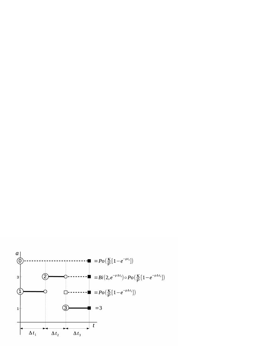
Figure 1: Illustration of Example 2.3

From the Theorem and (4), we get that

Corollary 2.4.

(i) Conditional density of $(e_{i},\Delta t_{i}|\xi_{[i-1]})$ is given by

$$f_{i}(\tau,e|\xi_{[i-1]})=\gamma_{i-1}^{-1}\exp\{-\gamma_{i-1}\tau\}\pi_{i}(e),$$

(ii) conditional density of $(a_{[i]},q_{[i]})|\xi_{[i-]}$ is given by

$$g_{i}(a,q|\xi_{[i-]})\\ =\begin{cases}\mathbf{1}[q=A^{a}_{[i-1]}+1]&\text{on $[b_{[i-1]}<a\leq a_{[i-1]},e_{i}=\mathrm{SLO}(a)]$}\\ \mathbf{1}[q=q_{[i-1]}-1]&\text{on $[a=a_{[i-1]},e_{i}\in\{\mathrm{CA}(a_{[i-1]}),\mathrm{BMO}\},q_{[i-1]}>1]$}\\ \omega_{a,q,i}\prod\limits_{\pi=a_{[i-1]}+1}^{a-1}(1-\varpi_{\pi,i})^{\nu_{\pi,i}}e^{-\epsilon_{\pi,i}-\iota_{\pi,i}}&\text{on $[a_{[i-1]}<a,e_{i}\in\{\mathrm{CA}(a_{[i-1]}),\mathrm{BMO}\},q_{[i-1]}=1]$}\\ \mathbf{1}[q=q_{[i-1]},a=a_{[i-1]}]&\text{otherwise},\end{cases}$$

where $\mathbf{1}$ denotes indicator function and

$$\omega_{p,q,i}=\begin{cases}\mathbb{P}[\mathrm{Bi}(\nu_{p,i},\varpi_{p,i})\circ\mathrm{Po}(\epsilon_{p,i}+\iota_{p,i})=q]&a_{[i-1]}<p\leq n,\\ \mathbf{1}[q=0]&a=n+1.\end{cases}$$

(iii) conditional density of $(a_{[i]},q_{[i]},e_{i},\Delta t_{i})$ given $\xi_{[i-1]}$ is given by

$$h_{i}(a,q,e,t|\xi_{[i-1]})=g_{i}(a,q|e,t,\xi_{[i-1]})f_{i}(e,t|\xi_{[i-1]}).$$

Remark 1.

As the definitions of $B$ and $A$ are symmetric, formulas for the (conditional) distribution of $(b,r)$ are symmetric to those for $(a,q)$. Moreover, as changes of $(a,q)$ and $(b,r)$ are mutually exclusive almost sure, i.e.,

$$[\text{$(a,q)$ changes at $t$}]\Rightarrow[\text{$(b,r)$ does not change at $t$}]$$

almost sure and vice versa, $(b,r)$ is conditionally constant given events which cause changes of $(a,q)$ (and vice versa) so the conditional distribution of $x_{[i]}|\xi_{[i-]}$ is uniquely determined by Corollary 2.4 and a formula for $(b,r)$.

In the rest of the paper, we shall deal only with the ask side, i.e., with $(A,a,q)$, leaving $(B,b,q)$ aside due to the symmetry.

Because density $h_{i}$ depends on all the parameters related to $A$ (i.e., $\kappa,\rho,\theta,\iota$), it is straightforward to estimate these parameters by Maximum Likelihood based on $h_{i}$ and a sample from ($\Delta t_{[i]},e_{[i]},a_{[i]},q_{[i]}$). Moreover, if we put

$$\iota\equiv 0$$ (5)

and, quite realistically, assume that $\kappa$ and $\rho$ depend only on a distance to the ask, i.e.,

$$\kappa(a,b,p)=\tilde{\kappa}(a-p),\qquad\rho(a,b,p)=\tilde{\rho}(a-p)$$ (6)

for some $\tilde{\kappa}$ and $\tilde{\rho}$, and that the “inside-the-book” intensities

$$\tilde{\kappa}|_{\{1,2,\dots\}},\quad\tilde{\rho}|_{\{1,2,\dots\}},$$ (7)

depend on different parameters than the “spread” intensities

$$\theta,\quad\tilde{\kappa}|_{\{0,-1,-2,\dots\}},\quad\tilde{\rho}|_{\{0,-1,-2,\dots\}},$$ (8)

then the estimation of the “ask-side” parameters could be split into the estimation of the parameters underlying (8), based on $f_{i}(\Delta t_{i},e_{i})_{i\in\mathbb{N}}$, and that of the parameters underlying (LABEL:eq:parssob), based on $g_{i}(a_{[i]},q_{[i]})_{i\in\mathbb{N}}$. In the present paper, only the latter case of an estimation is discussed.

3 Generalised Model

Despite the popularity of the ZI models, there is no doubt that they are too rough and neglect many aspects of real-life trading. The most obvious issues in this respect are two:

1. the volumes are non-unit in reality,

2. agents, at least sometimes, act strategically rather than in a random way.

To deal with (i), authors of ZI models usually argue that the sizes of a majority of orders are one-lot and, when an order is larger, it may be imagined that several subsequent one-lot orders have been issued. However, this simplification may be tolerable only in the case of limit orders (if the order book is observed only at certain time instants then larger orders are indeed interchangeable with several subsequent unit ones) but it is unacceptable for non-unit market orders which could not be imaginatively split without a serious violation of the assumption that their arrival intensity is constant.

To justify the ZI models against (ii), it is usually argued that the strategic reasoning is so complex that taking it as random is less evil than constructing wrong models. This argument, however, has a drawback, too: no matter how reasonable it may sound, one still has to deal with empirical phenomena stemming from (bounded) rationality, such as shifts and rapid insertions and cancellations of orders (especially quotes) in response to changes of the book.

To meet those issues, the setting defined in Section 2.1 might be generalised by assuming tbat

M

volumes of market orders are possibly non-unit,

S1

once a (unit) limit order stops to be a quote due to an in-spread sell limit order, it is, with probability $1-\eta$, immediately cancelled or shifted to the position of the new quote,

S2

once a quote jumps out of the spread, there is a non-zero probability that the move was caused not by a market order or cancellation but by a shift of the quote.

Moreover, to give more freedom to modelling of (possibly complex) behaviour of the quotes, it is allowed that

D

the distribution of $\Delta t_{i},e_{i}|\xi_{[i-1]}$ is arbitrary and, moreover, $q$ and $r$ may jump by more than one unit.

The list of events potentially changing $x$ at $t_{i}$ is newly as follows:

code	description
$\mathrm{BMO}(z)$	a buy market order of volume $z$
$\mathrm{SLO}(p,z)$	a sell limit order with price $b_{[i-1]}<p\leq a_{[i-1]}$ and size $z$ put into the spread
$\mathrm{CA}(a_{[i-1]},z)$	a cancellation of $z$ orders of the ask
$\mathrm{SAL}(z,a)$]	a shift of $z$ orders with price $a_{[i-1]}$ to tick $a_{[i-1]}-a$, $a>0$
$\mathrm{SAR}(z,a)$]	a shift of $z$ orders with price $a_{[i-1]}$ to tick $a_{[i-1]}+a$, $a>0$

plus symmetric events concerning $b$.

Even though, given this generalisation, (i) of Theorem 2.2 ceases to be true, its Assertions (ii) and (iii) would keep holding with $\eta\varpi_{p,i}$ instead of $\varpi_{p,i}$ if it is additionally assumed that

• the volumes of market orders are i.i.d. random, independent of all the past and the present events on the market

• the (Bernoulli) variables indicating the shifts are mutually independent, independent of the past and the present events on the market.

What does change, however, is the distribution of quote jumps outside of the spread after the ask is depleted, which are now non-zero if and only if

$$[e_{i}\in\{\mathrm{BMO}(z),\mathrm{CA}(q_{[i-1]}),\mathrm{SAR}(z,a)\},z\geq q_{[i-1]},a>0],$$ (9)

in which case

$$(a_{[i]},q_{[i]})=(a,q)\Leftrightarrow\begin{cases}M_{a,i}\leq s_{i},M_{a,i}+A^{a}_{[i-]}=s_{i}+q,&a\leq n,\\ M_{n+1,i}\leq s_{i}&a=n+1,q=0,\end{cases}$$

where

$$M_{a,i}=\sum_{j=a_{[i-1]}+1}^{a-1}A^{j}_{[i-]}$$

is the total number of the orders in the book between the former and the present value of the ask and

$$s_{i}=\begin{cases}z-q_{[i-1]}&\text{if $e_{i}=\mathrm{BMO}(z)$,}\\ -z&\text{if $e_{i}=\mathrm{SAR}(z,a)$ for some $a$,}\\ 0&\text{if $e_{i}=\mathrm{CA}(a_{[i-1]}).$}\end{cases}$$

is the number of the orders the particular change would like to “eat” from the inside of the book.

As, by (ii) and (iii) of (the modified version of) Theorem 2.2,

$$M_{a,i}|\xi_{[i-]}\sim\mathrm{Bi}(\nu_{a_{[i-1]}+1,i},\eta\varpi_{a_{i-1}+1,i})\circ\dots\circ\mathrm{Bi}(\nu_{a-1,i},\eta\varpi_{a-1,i})\circ\mathrm{Po}\left(\sum_{j=a_{[i-1]}+1}^{a-1}[\epsilon_{j,i}+\iota_{j,i}]\right)$$

and, by (iii) of the Theorem, $A^{a}_{[i-]}$ is conditionally independent of $M_{a,i}$ given $\xi_{[i-]}$, we are getting

Corollary 3.1.

On set (9), the distribution of $(a_{[i]},q_{[i]})|\xi_{[i-]}$ is given by density

$$\tilde{g}_{i}(a,q|\xi_{[i-]})=\begin{cases}\sum_{j=0}^{s_{i}}\mathbb{P}[M_{i}=j|\xi_{[i-]}]\mathbb{P}[A^{a}_{[i-]}=s_{i}+q-j|\xi_{[i-]}]&a_{[i-1]}<a\leq n,\\ \mathbb{P}[M_{i}\leq s_{i}|\xi_{[i-]}]&a=n+1,q=0.\end{cases}$$

Remark 2.

As both the value of the ask and its volume are uniquely determined by $\xi_{[i-]}$ outside set (9), the distribution of $(a_{[i]},q_{[i]})|\xi_{[i-]}$ is Dirac outside set (9).

Thus, if we keep assuming (5) and (6), we may estimate parameters underlying $\tilde{\kappa}|_{\{1,2,\dots\}}$ and $\tilde{\rho}|_{\{1,2,\dots\}}$ together with $\eta$ by means of MLE based on $\tilde{g}_{i}$; as it could be checked in Appendix B, the asymptotic properties of the estimator are not harmed by the generalisation provided that the generalised process is ergodic, which may be guaranteed, e.g., by requiring that

E

$q_{t}+r_{t}$ is stochastically dominated by a Markov chain with a zero recurrent state.

Under this assumption, Proposition 2.1 keeps holding because none of the generalisations, except for D, which is treated by E, increase the total number of orders in $\Xi$ in comparison with the ZI.

Remark 3.

Unlike in the unit-volume ZI model, price impact may be predicted in the GZI model: denoting $m_{i}$ the impact of a trade with volume $z$ at time $t$, we have

$$\mathbb{P}[m_{i}(z)=m|\xi_{[i-1]}=\xi,t_{i}=t,,e_{i}=\mathrm{BMO}(z)]=\mathbb{P}[\Delta a_{[i]}=m|\xi_{[i-1]}=\xi,t_{i}=t,e_{i}=\mathrm{BMO}(z)]\\ =\sum_{q=0}^{\infty}\tilde{g}_{i}(a_{[i-1]}+m,q|\xi_{[i-1]}=\xi,t_{i}=t,e_{i}=\mathrm{BMO}(z)).$$

4 Empirical Evidence

4.1 Data

For our empirical analysis, tick-by-tick trade and quote data was used, i.e., values

$$(x_{[i]},\tau_{[i]})_{i\in\mathbb{N}}$$

where $\tau_{[i]}$ is an amount traded at $t_{i}$, defined by

$$\tau_{[i]}=\begin{cases}z&e_{i}=\mathrm{SMO}(z)\\ -z&e_{i}=\mathrm{BMO}(z)\\ 0&\text{otherwise}.\end{cases}$$

In particular, data of six stocks

• Exxon Mobile (XOM)

• Microsoft (MSFT),

• General Electric (GE)

• MarketAxess Holdings (MKTX)

• J2 Global (JCOM)

• American Realty Investors (ARL)

from nine US electronic markets

• NASDAQ OMX BX

• NSE

• Chicago

• NYSE

• ARCA

• NASDAQ T

• CBOE

• BATS

• ISE

from ten months starting from March $2009$ were analysed.

Our choice of the titles was done so as to cover both “large” and the “smaller” stocks. The first three ones - XOM, MSFT and GE - belong to the top ten companies by market capitalization and usually exhibit large trading volumes. MKTX and JCOM, on the ather hand, are usually ranked as “small caps” (having market capitalization around $1 bilion) with moderate trading volumes. Company ARL, belonging to the category of “micro caps” (capitalisation around $100 million), could be counted among illiquid stocks.

As to the markets, we did not pre-select which of them to analyse; contrarily, all the markets were included on which the examined stocks were traded and for which at least some data were available- the only exception is NASDAQ ADF, which is a platform for recording trades rather than a limit order market (see FINRA (2015)).

As the trade data (process $\tau$) came from a different data source than the quote data (process $x$), it was necessary to algorithmically match individual trades with the L1 data changes in which our algorithm, designed for that purpose, succeeded in about 70 percent of trades (the rest could not be uniquely attributed to any L1 change ). This fact, however, did not harm the estimation other way than by decreasing the sample size.

4.2 Estimation

For the actual estimation, only records originating between 9:40 a.m. and 3:30 p.m. were used when the process could be assumed to be near its stationary distribution; the inclusion of the ten-minute “warm-up” period following the opening at 9:30 also partially justifies our assumption (5).

When estimating within the ZI models, all the jumps of $a$ up could serve as a sample while, in the case of the GZI models, only the jumps of $a$ matched with trades were included; the reason for this restriction is that the jumps of $a$ caused by unpaired trades, shifts and cancellations could not be distinguished from each other in the L1 data, so the corresponding values of $s_{i}$ could not be determined. For each paired trade record, on the other hand, the value of $s_{i}$ may be obtained from the volume of the trade and from the (known) volume of the former ask.

For both the ZI and the GZI settings, and for each stock-market pair, the following estimation procedure was run: as its first step, a simple version of the model with

$$\tilde{\kappa}(\bullet)\equiv\kappa_{0},\quad\tilde{\rho}(\bullet)\equiv\rho_{0},\quad\rho_{0}>0,\quad\kappa_{0}>0\qquad(S)$$

(Smith et al. (2003) in its ZI variant), which we later call basic model, was estimated. Subsequently, three power tail models with $\tilde{\kappa}$ and $\tilde{\rho}$, defined by

$$\tilde{\kappa}(i)=\begin{cases}\kappa_{i-1}&i\leq n\\ \kappa_{n-1}(i-n)^{\alpha_{\kappa}}&i>n\end{cases}\quad\tilde{\rho}(i)=\begin{cases}\rho_{i-1}&i\leq n\\ \rho_{n-1}(i-n)^{\alpha_{\rho}}&i>n,\end{cases}\qquad(T_{n})\qquad\qquad n=1,2,3,$$

were estimated gradually. As a “true” model, the one was chosen in which all the parameters came out significant while the likelihood ratio comparing this model with the subsequent one came out insignificant.

Each estimation procedure was run on a sample of at most $5,000$ observations; even though there were many more observations available for a majority of the stock-market pairs, a restriction had to be made due to the large time requirement of the estimation, caused by complex formulas for conditional densities involved. In case that the optimisation algorithm could not find maximum of the ML function within a time limit of $2,500$ sec (approx. $42$ min) for none of the four variants of the model, the procedure was repeated once more with a sample of size $1,000$.

The prediction power of each model $m$ was evaluated by

$$P_{m}=1-\frac{\sum_{i=N}^{N+M}|a_{[i]}^{+}-\mathbb{E}(a_{[i]}^{+}|\xi_{[i-]})|}{\sum_{i=N}^{N+M}|a_{[i]}^{+}-\bar{a^{+}}_{N}|}$$

where $N$ is a sample size, $M\doteq N/10$ is the number of out-of-sample observations, $a^{+}_{1},\dots,a^{+}_{M+N}$ are the magnitudes of the jumps of $a$ up, $\bar{a}^{+}_{N}$ is their average and where the conditional expectation in the numerator was computed by means of the estimated parameters. By its construction, $P_{m}$ can be understood as a percentage improvement in comparison with a naive prediction of the out-of-spread jumps by their mean. In the GZI setting, $P_{m}$ may also be seen as a measure of accuracy of the market impact prediction.

For automation of the whole procedure including matching of trades, and the model selection, a C++ package has been developed by the author, using the NLOPT library, namely LBFGS and BOBYQUA optimisation algorithms, to compute maxima of the ML functions. A source code of the package is available at https://github.com/cyberklezmer/fepp under branch qf15.

4.3 Results

Results of the estimation procedure of the ZI modelsd for the “big-cap” stocks XOM, MSFT and GE are summarised in Table 1. It may be seen that 21 out of all the 27 estimations were successful in the sense that a significant model was found, which exhibits a positive improvement (measured by $P_{m}$). Out of the “failed” cases, four times a significant model was found giving a negative $P_{m}$, once the time limit was reached even with a reduced sample, and once no data was available.

Out of all the 21 successful instances, the basic model $(S)$ was chosen nine times, the simplest tail model $(T_{1})$ six times and model $(T_{2})$ six times; model $(T_{3})$ never came out significant within the time limit. Higher $P_{m}$’s values in comparison with a basic model were reached in only seven out of the 12 cases when a tail model was selected, while the basic model came out better in two cases; in the three remaining cases, the $P_{m}$ was identical up to two decimal digits. Even though, on average, the tail model performed better, the difference was not found statistically significant according to a Wilcoxon test. Detailed results of this estimation can be found in Appendix C.1.

Summary results for the GZI model for big-caps may be found in Table 2. Here, the estimation was successful in 21 out of 25 cases with at least some data, three times the time-out was reached; $P_{m}$ came out negative in one case.

In order to answer the question whether it is worth using the more complicated GZI model rather than the ZI one, the estimation procedure was run for ZI models once more using the same samples as those used for the GZI ones (i.e., only the changes with trades matched); the corresponding results are displayed in the second column below each stock. Out of the 20 cases when both estimations were successful, eight times the GZI model reached a higher $P_{m}$ while three times $P_{m}$ was higher for the ZI model; nine times $P_{m}$ was the same up to two decimal digits. Again, it could not be statistically proved that the GZI model performs significantly better.

Detailed results of the GZI estimation may be found in Appendix C.2 (the GZI models) and Appendix C.3 (their ZI counterparts).

Tables 3 and 4 summarise estimates of tail exponents of $\tilde{\kappa}$ and $\tilde{\rho}$. It may be seen that a dispersion of the values of $\alpha_{\kappa}$ is great; however, their average $-2.3(0.41)$ is not far from present empirical evidence (see, e.g., Chakraborti et al. (2011a), III.C). The results for tail exponents of $\tilde{\rho}$, which have never been statistically estimated yet to the best of the author’s knowledge, are similar to the case of $\alpha_{\kappa}$, with average value $-2.48(0.42)$.

Results of the estimation of the small caps MKTX, JCOM and the micro-cap ARL may be found in Table 5 and Table 6. For the small caps, the ZI model was successful for 10 of 13 pairs with sample size at least $N>20$, once a negative $P_{m}$ was reached, two times the optimization failed. For ARL, the procedure was successful only once (with a disappointing prediction power) with all of the failures due to failed optimizations. A closer look to the results suggests two possible causes of the failures: small sample sizes and/or large average jumps of $a$, causing large evaluation times of the densities (see Appendix C for detailed values). The situation is not much better in the case of GZI models either: small caps are successful in 7 out of 9 cases, ARL is only once half-way successful out of three cases. Results of a comparison of more complex ZI models with their basic variant are similar to those of the big-caps: out of 8 cases when the comparison is possible, more complex models won three times, four times the basic model was more successful, once the results were the same. Similarly, from 8 comparisons of GZI and ZI variants of the model, the GZI variant was more successful four times, the ZI one three times, once the results were equal.

	XOM	MSFT	GE
NASDAQ OB	$T_{1}(<0)$	$T_{1}(0.70,0.70)$	$S(0.48)$
NSE	$T_{2}(0.91,0.90)$	$T_{2}(0.89,0.87)$	$T_{1}(0.76,0.76)$
Chicago	$T_{2}(0.47,n/a)^{-}$	$S(0.93)$	$T_{1}(0.76,0.71)$
NYSE	$S(0.33)$	$\times$	$S(0.53)$
ARCA	$T_{1}(0.92,0.91)$	$S(-\infty)^{\star}$	$t$
NASDAQ T	$T_{1}(0.53,0.53)$	$S(1.00)^{\star}$	$S(-\infty)^{\star}$
CBOE	$S(<0)$	$T_{2}(0.35,0.36)$	$S(0.67)$
BATS	$T_{2}(0.86,0.83)$	$S(1.00)$	$S(0.00)^{\star}$
ISE	$T_{2}(0.66,0.67)$	$S(0.66)$	$T_{1}(0.94,0.93)^{\star}$

Table 1: Results for ZI. Notation: $m(p,p_{0})$ - model $m$ was selected with $P_{m}=p$ and with $P_{S}=p_{0}$, minus sign - sample less than $5000$ was available, $\star$ - a reduced sample used, $t$ - time limit reached when without finding a result, $\times$ - less than $20$ observations were available.

	XOM		MSFT		GE
	GZI	ZI	GZI	ZI	GZI	ZI
NASDAQ OB	$T_{2}(0.19)$	$T_{2}(0.17)$	$T_{1}(0.68)$	$T_{1}(0.66)$	$T_{1}(0.74)$	$S(0.74)$
NSE	$T_{1}(0.70)^{\star}$	$T_{1}(0.69)^{\star}$	$T_{2}(0.38)$	$T_{2}(0.29)$	$S(0.33)$	$t$
Chicago	$T_{2}(0.35)^{-}$	$T_{2}(0.34)^{-}$	$T_{2}(0.49)^{-}$	$T_{1}(0.51)$	$T_{1}(0.79)$	$T_{1}(0.79)$
NYSE	$S(0.17)$	$S(0.13)$	$\times$	$\times$	$S(1.00)^{\star}$	$S(1.00)^{\star}$
ARCA	$T_{2}(0.84)$	$T_{2}(0.84)$	$t$	$S(0.00)^{\star}$	$t$	$t$
NASDAQ T	$S(0.74)$	$T_{1}(0.74)$	$\times$	$\times$	$t$	$t$
CBOE	$T_{2}(<0)^{-}$	$T_{2}(<0)^{-}$	$T_{2}(0.72)^{-}$	$S(0.68)^{-}$	$T_{2}(0.23)$	$T_{2}(0.23)$
BATS	$T_{1}(0.31)$	$T_{1}(0.60)$	$S(0.00)^{\star}$	$S(0.00)^{\star}$	$S(0.00)^{\star}$	$S(0.00)^{\star}$
ISE	$T_{1}(0.44)^{\star}$	$S(0.42)^{\star}$	$T_{1}(0.96)^{\star}$	$T_{1}(0.96)^{\star}$	$S(0.36)^{\star}$	$S(0.42)^{\star}$

Table 2: Results for GZI. Notation: $m(p)$ model $m$ was used with $P_{m}=p$, minus sign - sample with less than $5,000$ available, $\star$ - a reduced sample used, $t$ - time limit reached without finding a result, $\times$ - less than $20$ observations were available

	XOM		MSFT		GE
	ZI	GZI	ZI	GZI	ZI	GZI
NASDAQ OB	$-5.49$	$-2.60$	$-0.38$	$-0.48$	$n/a$	$-4.15$
NSE	$-1.11$	$-2.83$	$-1.30$	$-2.64$	$-0.12$	$n/a$
Chicago	$-2.31$	$-2.28$	$n/a$	$-0.75$	$-9.72$	$-1.47$
NYSE	$n/a$	$n/a$	$\times$	$\times$	$n/a$	$n/a$
ARCA	$-2.18$	$-1.75$	$n/a$	$t$	$t$	$t$
NASDAQ T	$-0.84$	$n/a$	$n/a$	$\times$	$n/a$	$t$
CBOE	$n/a$	$-1.70$	$-0.97$	$-0.34$	$n/a$	$-2.12$
BATS	$-1.15$	$-4.84$	$n/a$	$n/a$	$n/a$	$n/a$
ISE	$-1.18$	$-2.76$	$n/a$	$-6.76$	$-0.26$	$n/a$

Table 3: Estimated values of $\alpha_{\kappa}$. Notation: $n/a$ - only model $S$ came out significant, $t$ - time limit reached, $\times$ - no data available.

	XOM		MSFT		GE
	ZI	GZI	ZI	GZI	ZI	GZI
NASDAQ OB	$-5.37$	$-2.60$	$-0.26$	$-0.60$	$n/a$	$-4.22$
NSE	$-1.84$	$-2.89$	$-0.89$	$-2.31$	$-0.61$	$n/a$
Chicago	$-2.13$	$-3.22$	$n/a$	$-1.94$	$-8.28$	$-1.77$
NYSE	$n/a$	$n/a$	$\times$	$\times$	$n/a$	$n/a$
ARCA	$-1.77$	$-0.77$	$n/a$	$t$	$t$	$t$
NASDAQ T	$-0.67$	$n/a$	$n/a$	$\times$	$n/a$	$t$
CBOE	$n/a$	$-2.21$	$-0.03$	$-9.24$	$n/a$	$-3.39$
BATS	$-0.38$	$-4.59$	$n/a$	$n/a$	$n/a$	$n/a$
ISE	$-0.94$	$-2.43$	$n/a$	$-3.56$	$-0.66$	$n/a$

Table 4: Estimated values of $\alpha_{\rho}$. Notation: $n/a$ - only model $S$ came out significant, $t$ - time limit reached, $\times$ - no data available.

	MKTX	JCOM	ARL
NASDAQ OB	$f^{\star}$	$T_{1}(0.06,0.06)$	$\times$
NSE	$\times$	$f^{\star}$	$\times$
Chicago	$\times$	$\times$	$\times$
NYSE	$\times$	$\times$	$f$
ARCA	$T_{2}(0.40,0.45)$	$T_{2}(0.18,0.17)$	$f^{\star}$
NASDAQ T	$T_{2}(0.44,0.46)$	$T_{2}(0.38,0.37)$	$S(0.08)^{-}$
CBOE	$S(0.92)^{\star}$	$T_{2}(<0,<0)$	$f^{-}$
BATS	$T_{2}(0.13,0.35)$	$T_{2}(0.60,0.52)$	$f^{-}$
ISE	$S(0.31)^{\star}$	$T_{2}(0.39,0.49)$	$f^{-}$

Table 5: Results for ZI of the small caps. Notation: $f$ - optimization failed, for the rest, see Table 1.

	MKTX		JCOM		ARL
	GZI	ZI	GZI	ZI	GZI	ZI
NASDAQ OB	$\times$	$\times$	$T_{2}(0.78)^{-}$	$T_{1}(0.79)^{-}$	$\times$	$\times$
NSE	$\times$	$\times$	$\times$	$\times$	$\times$	$\times$
Chicago	$\times$	$\times$	$\times$	$\times$	$\times$	$\times$
NYSE	$\times$	$\times$	$\times$	$\times$	$S(<0)^{-}$	$T_{2}(<0)^{-}$
ARCA	$T_{2}(0.31)^{-}$	$T_{2}(0.25)^{-}$	$S(0.08)$	$T_{2}(0.04)$	$f^{-}$	$f^{-}$
NASDAQ T	$\times$	$\times$	$\times$	$\times$	$S(<0)^{-}$	$T_{1}(0.49)^{-}$
CBOE	$S(1.00)^{-}$	$S(1.00)^{-}$	$T_{1}(0.29)^{-}$	$T_{1}(0.25)^{-}$	$\times$	$\times$
BATS	$S(0.41)^{-}$	$S(0.39)^{-}$	$T_{2}(0.65)$	$S(0.66)$	$\times$	$\times$
ISE	$S(<0)^{-}$	$S(<0)^{-}$	$S(<0)^{-}$	$S(<0)^{-}$	$\times$	$\times$

Table 6: Results for GZI of the small caps. Notation: $f$ - optimization failed, for the rest, see Table 2

5 Conclusions

A setting covering many of the existing zero intelligence (ZI) models and its generalisation allowing for non-unit market orders and shifts of quotes (GZI) were introduced. Several variants of both the ZI and GZI settings, differing in their complexity, were tested on trade and quote data for 54 real-life stock-market pairs. It was found that, especially for liquid stocks, both the ZI and GZI models came out significant with a substantial prediction power; however, their more complicated variants did not produce significantly better predictions in comparison with a simple model with constant intensities. Finally, as the rewults of the ZI and the GZI variants are comparable, our suggestion is to use the GZI models which are more realistic and are capable of predictions of market impact.

Appendix A Proof of Theorem 2.2

Before starting the proof, recall that that a Markov chain $X$ on $\mathbb{R}^{+}$ is called immigration and death process with immigration intensity $\kappa$ and death intensity $\rho$ and with initial population $A$ (we abbreviate this by $\mathcal{I}(\kappa,\rho,A)$) if its transition matrix $\Lambda=(\lambda_{i,j})$ has zero components except of $\lambda_{j,j+1}=\kappa$, $\lambda_{j,j-1}=j\rho$, $j>0$ and if $X_{0}=A$. Notice also that number of customers in an $M/M/\infty$ in queuing theory model follows an $\mathcal{I}$ process. It is well known (see, e.g., Mandjes and Żuraniewski (2011), Section 2) that, for any positive $t$,

$$\mathcal{I}(\kappa,\rho,A)_{t}\sim\mathrm{Po}\left(\frac{\kappa}{\rho}[1-\exp\{-\rho t\}]\right)\circ\mathrm{Bi}(A,\exp\{-\rho s\}).$$ (10)

Further, let us introduce the following (re)formulation of process $\Xi$ restricted to time interval $(0,t_{1}]$, which will be used repeatedly in the subsequent proof: Let $u^{1},v^{1},u^{2},v^{2},\dots,u^{n},v^{n}$ be independent uniform variables, independent of $\Xi_{0}$. By Kallenberg (2002), Theorem 6.10, there exist mappings $U^{1},V^{1},\dots,U^{n},V^{n}$ from $\mathbb{N}_{0}^{n}\times[0,1]$ to the space of stochastic processes on $\mathbb{R}^{+}$ such that, for each $\pi$, $U^{\pi}(A_{0},u^{\pi})|\Xi_{0}\sim\mathcal{I}(\kappa_{\pi,0},\rho_{\pi,0},A^{\pi}_{0})$ and $V^{\pi}(B_{0},v^{\pi})|\Xi_{0}\sim\mathcal{I}(\lambda_{\pi,0},\sigma_{\pi,0},B^{\pi}_{0})$. By Kallenberg (2002), Proposition 6.13., $U^{1},V^{1},U^{2},V^{2},\dots,U^{n},V^{n}$ are mutually conditionally independent given $\Xi_{0}$, so we may assume, without a change of distributions,

$$A_{t}=(U_{t}^{1},\dots,U_{t}^{n}),\qquad B=(V_{t}^{1},\dots,V_{t}^{n})\qquad\text{on $[t\leq t_{1}]$}.$$ (11)

(to see it, check definitions (1) and (2)).

Using this reformulation and noting that both $e_{1}$, $\Delta t_{1}$ are functions of $(U^{\pi},V^{\pi})_{\pi\leq a_{0}}$, we see that

$$(t_{1},e_{1}){\perp\perp}_{\Xi_{0}}(U^{\pi})_{\pi>a_{i}}$$ (12)

where $A{\perp\perp}_{C}B$ denotes conditional indepdence of $A$ and $B$ given $C$.

Because, by the definition of the ask, $A^{1}_{[i-]}=A^{2}_{[i-]}=\dots=A^{a_{0}-1}_{[i-]}=0$ and $A^{a_{0}}_{[i-]}=q_{0}$, i.e, $A^{1}_{[i-]},\dots,A^{a_{0}}_{[i-]}$ are conditionally constant, we have, for any $s_{1},s_{2},\dots,s_{n}$,

$$\mathbb{P}[A^{1}_{[1-]}=s_{1},A^{2}_{[1-]}=s_{2},\dots,A^{n}_{[1-]}=s_{n}|e_{1},t_{1},\Xi_{0}]\\ =\mathbf{1}[s_{1}=s_{2}=\dots=s_{a_{0}-1}=0,s_{a_{0}}=q_{0}]\cdot\mathbb{P}[U^{a_{0}+1}_{t_{1}-}=s_{a_{0}+1},\dots,U^{n}_{t_{1}-}=s_{n}|e_{1},t_{1},\Xi_{0}]\\ =\mathbf{1}[s_{1}=s_{2}=\dots=s_{a_{0}-1}=0,s_{a_{0}}=q_{0}]\cdot\prod_{\pi=a_{0}+1}^{n}\mathbb{P}[U^{\pi}_{t_{1}}=s_{\pi}]$$ (13)

where the last “=” follows from Hoffmann-Jørgenson (1994), (6.8.14) (with $R=(u^{a_{0}+1},u^{a_{0}+2},\dots,u^{n})$ and $S=(e_{1},t_{1},\Xi_{0})$) and from the fact that the jumps of $U$’s do not coincide with probability one (which guarantees that $U^{\pi}_{t_{1}}=U^{\pi}_{t_{1}-}$, $\pi>a_{0}$, almost sure).

As a first step of proving the assertions of the Theorem, let us deal with one-step-ahead distribution $\mathbb{P}[(\Delta t_{i},e_{i},A_{[i-]})\in\bullet|\Xi_{[i-1]}]$:

Proposition A.1.

(i) For any $\tau$ and $e$,

$$\mathbb{P}[\Delta t_{i}>\tau,e_{i}=e|\Xi_{[i-1]}]=\exp\{-\gamma_{i-1}\tau\}\pi_{i}(e).$$

(ii) For any $p$,

$$A^{p}_{[i-]}|e_{i},\Delta t_{i},\Xi_{[i-1]}\sim\begin{cases}\mathrm{\boldsymbol{\delta}}_{0}&\text{on $[1\leq p<a_{[i-1]}]$}\\ \mathrm{\boldsymbol{\delta}}_{q_{[i-1]}}&\text{on $[p=a_{[i-1]}]$}\\ \mathrm{Po}\left(\phi_{p,i-1}(1-\delta_{p,i-1})\right)\circ\mathrm{Bi}\left(A_{[i-1]}^{p},\delta_{p,i-1}\right)&\text{on $[a_{[i-1]}<p\leq n]$}.\\ \end{cases}$$

(iii) For any $p$,

$$A^{p}_{[i]}|e_{i+1},\Delta t_{i+1},x_{[i]},\Delta t_{i},\Xi_{[i-1]}\\ \sim\begin{cases}\mathrm{\boldsymbol{\delta}}_{A_{[i]}}&\text{on $[1\leq p\leq\max(a_{[i]},a_{[i-1]})]$}\\ \mathrm{Po}\left(\phi_{p,[i-1]}(1-\delta_{p,i-1})\right)\circ\mathrm{Bi}\left(A_{[i-1]}^{p},\delta_{p,i-1}\right)&\text{on $[\max(a_{[i]},a_{[i-1]})<p\leq n]$}.\end{cases}$$

Proof.

Thanks to the homogeneity of the process, we may assume $i=1$.

(i) It follows from textbook knowledge that $\Delta t_{1}$, being the first jump time of Markov chain $(V^{b_{0}},U^{b_{0}+1},V^{a_{0}+1},\dots,U^{a_{0}})$, is exponential with rate $\gamma_{0}$, while $e_{i}$, coding a type of the chain’s first jump, is (conditionally w.r.t. $\Xi_{0}$) independent of $\Delta t_{1}$ with probabilities of particular events being equal to the rates of the events’ intensities to $\gamma_{0}$, which is formally expressed by (i).

(ii) The formula follows from (13) and (10).

(iii) Let $1\leq j,k\leq n$ and put $S_{j,k}=[a_{[1]}=j,a_{0}=k]$. Clearly,

$$x_{[1]}=\tilde{x}_{[1]}\qquad\text{on $S_{j,k}$},$$ (14)

where

$$\qquad\tilde{x}_{[1]}=(j,A^{j}_{[1]},\tilde{b},B^{\tilde{b}}_{[1]}),\qquad\tilde{b}=\max\{\pi<j:B^{\pi}_{[1]}>0\}.$$

Further, it follows from the dynamics of the process and from the almost sure exclusivity of jumps of $\Xi$ that

$$A_{[1]}=\tilde{A}\quad\text{on $S_{j,k}$},\qquad\tilde{A}=(r_{j,k},A^{j\vee k+1}_{[1-]},\dots,A^{n}_{[1-]}),\\ r_{j,k}=\begin{cases}(\underbrace{0,\dots,0}_{j\times},q_{[1]})&j\geq k\\ (\underbrace{0,\dots,0}_{j\times},q_{[1]},\underbrace{0,\dots,0}_{(k-j-1)\times},q_{0})&j<k.\\ \end{cases}$$ (15)

Now, because $(\Delta t_{1},\tilde{x}_{[1]})$ are functions of $U^{1},V^{1},\dots,U^{j},V^{j},\Xi_{0}$, we have $(\Delta t_{1},\tilde{x}_{[1]})\in\sigma(U^{1},V^{1},\dots,U^{j},V^{j},\Xi_{0})$ so we may use the Law of Iterated Expectation to get

$$\mathbb{P}[\tilde{A}\in\bullet|\tilde{x}_{[1]},\Delta t_{1},\Xi_{0}]=\mathbb{E}(\mathbb{P}[\tilde{A}\in\bullet|U^{1},V^{1},\dots,U^{j},V^{j},\Xi_{0}]|\tilde{x}_{[1]},\Delta t_{1},\Xi_{0})\\ =\mathbb{E}(\mathbb{P}[\tilde{A}\in\bullet|\Xi_{0}]|\tilde{x}_{[1]},\Delta t_{1},\Xi_{0})=\mathbb{P}[\tilde{A}\in\bullet|\Xi_{0}]=p_{j,k}(\bullet;t_{1},\Xi_{0},r_{j,k})\quad\text{on $S_{j,k}$},\\ p_{j,k}(s_{1},\dots,s_{n};t,\Xi,r)=\mathbf{1}[r_{1}=s_{1},\dots,r_{j\vee k}=s_{j\vee k}]\prod_{\pi=j\vee k+1}^{n}\mathbb{P}[U^{\pi}(\Xi)_{t}=s_{\pi}].$$ (16)

(at the third “=”, we have used Proposition 6.6 of Kallenberg (2002), the fourth one is due to measurability of the inner term w.r.t. the condition of the expectation, the fifth one is due to (13)).

Now, by Local Property (Kallenberg (2002), Lemma 6.2) applied to (14), (15) and (16), we are getting that

$$\mathbb{P}[A_{[1]}\in\bullet|x_{[1]},\Delta t_{1},\Xi_{0}]=p_{a_{[1]},a_{0}}(\bullet;t_{1},\Xi_{0},(A^{1}_{[1]},A^{2}_{[1]},\dots,A_{[1]}^{a_{[1]}\vee a_{0}}))$$ (17)

on each $S_{j,k}$ and, as the $S_{j,k}$’s cover all the underlying probability space, the relation holds universally.

Finally, by the strong Markov property of $\Xi$ (guaranteed, e.g., by Kallenberg (2002), Theorem 12.14.), we get

$$\mathbb{P}[\Delta t_{2}>\tau,e_{2}=e|\Xi_{[1]},x_{[1]},\Delta t_{1},\Xi_{0}]=\mathbb{P}[\Delta t_{2}>\tau,e_{2}=e|\Xi_{[1]}]$$

which is, by Proposition 6.6. of Kallenberg (2002), equivalent to

$$\Delta t_{2},e_{2}{\perp\perp}_{x_{[1]},\Delta t_{1},\Xi_{0}}\Xi_{[1]}$$

implying, by the same Proposition with switched variables,

$$\mathbb{P}[\Xi_{[1]}\in\bullet|e_{2},\Delta t_{2},x_{[1]},\Delta t_{1},\Xi_{0}]=\mathbb{P}[\Xi_{[1]}\in\bullet|x_{[1]},\Delta t_{1},\Xi_{0}]$$

which, together with (17), proves (iii). ∎

Proof of the Theorem

Ad (i)

By the Law of Iterated Expectation, the strong Markov property of $\Xi$, and Proposition A.1 (i), it follows

$$\mathbb{P}[\Delta t_{i}>\tau,e_{i}=e|\xi_{[i-1]}]=\mathbb{E}[\mathbb{P}[\Delta t_{i}>\tau,e_{i}=e|\Xi_{[i-1]},\xi_{[i-1]}]|\xi_{[i-1]}]\\ =\mathbb{E}[\mathbb{P}[\Delta t_{i}>\tau,e_{i}=e|\Xi_{[i-1]}]|\xi_{[i-1]}]=\mathbb{E}(\exp\{-\gamma_{i-1}\tau\}\pi_{i}(e)|\xi_{[i-1]})=\exp\{-\gamma_{i-1}\tau\}\pi_{i}(e)$$ (18)

(we could get rid of the outer conditional expectation at the last equality because its integrand is measurable with respect to its condition).

Ad (ii)

Before deriving the distribution of $A_{[i-]}$, let us formulate an auxiliary result:

Lemma A.2.

Let $A,B$ be random variables, let $\mathcal{F}$ be as $\sigma$-algebra and let $S\in\mathcal{F}$. If $B|\mathcal{F}\sim\mathrm{Po}(\epsilon)\circ\mathrm{Bi}(\nu,\varpi)$ on $S$ and $A|B,\mathcal{F}\sim\mathrm{Po}(\zeta)\circ\mathrm{Bi}(B,\delta)$ on $S$ for some $\mathcal{F}$-measurable variables $\epsilon,\nu,\varpi,\zeta,\delta$ then $A|\mathcal{F}\sim\mathrm{Po}(\zeta+\delta\epsilon)\circ\mathrm{Bi}(\nu,\delta\varpi)$ on $S$.

Proof.

Let $A_{0},B_{0},C_{1},D_{1},E_{1},C_{2},D_{2},E_{2}\dots$ be variables mutually conditionally independent given $\mathcal{F}$, such that, on $S$, $A_{0}|\mathcal{F}\sim\mathrm{Po}(\zeta)$, $B_{0}|\mathcal{F}\sim\mathrm{Po}(\epsilon)$, and, for each $i\in\mathbb{N}$, $C_{i}|\mathcal{F}\sim\mathrm{Bernoulli}(\delta)$, $D_{i}|\mathcal{F}\sim\mathrm{Bernoulli}(\delta)$, $E_{i}|\mathcal{F}\sim\mathrm{Bernoulli}(\varpi)$ (outside $S$, all the variables could be e.g., zero). Assume, without a change of the examined distributions, that $B=B_{0}+E_{1}+E_{2}+\dots+E_{\nu}$ and $A=A_{0}+A_{1}+A_{2}$ where $A_{1}=\sum_{i=1}^{B_{0}}C_{i}$, $A_{2}=\sum_{i=1}^{\nu}D_{i}E_{i}$. Clearly, $A_{2}$ is (conditionally) Binomial with parameters $\nu$ and $\delta\varpi$. Further, by Daley and Vere-Jones (2003), 2.3.4, $A_{1}|\mathcal{F}\sim\mathrm{Po}(\delta\epsilon)$. As $A_{0},A_{1},A_{2}$ are mutually conditionally independent given $\mathcal{F}$ (which is because each of them depends on independent variables) we get that $A=\mathrm{Po}(\zeta)\circ\mathrm{Po}(\delta\epsilon)\circ\mathrm{Bi}(\nu,\delta\varpi)$. The Lemma now follows from the fact that a convolution of two Poisson variables is again Poisson. ∎

Let $1\leq p\leq n$. First we prove, by induction, that, for any $k$,

$$A^{p}_{[k]}|\xi_{[(k+1)-]}\sim\mathrm{Po}(\epsilon_{p,k}+\iota_{p,k})\circ\mathrm{Bi}(\nu_{p,k},\varpi_{p,k}),\qquad\text{on $[a_{[k]}<p\leq n]$}.$$ (19)

First, we show that (19) holds for $k=0$: indeed, by Proposition A.1 (i) and Kallenberg (2002), Proposition 6.6., we get that $(t_{1},e_{1}){\perp\perp}_{x_{0}}\Xi_{0}$ (recall that $\xi_{[1-]}=x_{0}$), which, by the Proposition 6.6. and by (3), gives (19) for $k=0$.

Now, assume (19) to hold for $k-1$. Similarly as in (18), we get, by Proposition A.1, (iii), that

$$\mathbb{P}[A^{p}_{[k]}\in\bullet|A^{p}_{[k-1]},\xi_{[(k+1)-]}]\\ =\mathbb{E}(\mathbb{P}[A^{p}_{[k]}\in\bullet|A^{p}_{[k-1]}]|A^{p}_{[k-1]},\xi_{[(k+1)-]})=\mathbb{E}(\mathbb{P}[A^{p}_{[k]}\in\bullet|\Xi_{[k-1]},e_{k},\Delta t_{k}]|A^{p}_{[k-1]},\xi_{[k-]})\\ =\mathbb{P}\left[\mathrm{Po}\left(\phi_{p,k-1}(1-\delta_{p,k-1})\right)\circ\mathrm{Bi}\left(A_{[k-1]}^{p},\delta_{p,k-1}\right)\in\bullet\right]$$ (20)

giving, by Lemma A.2 applied to the induction hypothesis and (20), validity of (19) on $[a_{[k-1]}<p\leq n]$. As, on $[a_{[i-1]}=p]$, $A^{p}_{[k]}=q_{[k]}$ is conditionally constant, i.e.,

$$\mathbb{P}[A^{p}_{[k]}=\alpha|\xi_{[(k+1)-]}]=\mathbf{1}[\alpha=q_{[k]}]=\mathbb{P}[\mathrm{Bi}(A^{p}_{[k]},1)\circ\mathrm{Po}(0)=\alpha]$$

(19) is proved on $[a_{[i-1]}=p]$ because $k_{k}(p)=k$ on the set so $\epsilon_{p,k}=\iota_{p,k}=0$, $\varpi_{p,k}=1$ and $\nu_{p,k}=A^{p}_{[k]}$ on the set. As (19) on $[a_{[i-1]}>p]$ follows similarly (here, $A^{p}_{[k]}=0$), (19) is proved for $k$.

Having proved (19) for any $k$, we may proceed to (ii) of the Theorem: Let $1\leq p\leq n$. Similarly as above we get, using Proposition A.1 (ii),

$$\mathbb{P}[A^{p}_{[i-]}\in\bullet|A^{p}_{[i-1]},\xi_{[i-]}]=\mathbb{E}(\mathbb{P}[A^{p}_{[i-]}\in\bullet|\Xi_{[i-1]},\Delta t_{i},e_{i}]|A^{p}_{[i-1]},\xi_{[i-]})\\ =\mathbb{P}\left[\mathrm{Po}\left(\phi_{p,i-1}(1-\delta_{p,i-1})\right)\circ\mathrm{Bi}\left(A_{[i-1]}^{p},\delta_{p,i-1}\right)\in\bullet\right]\qquad\text{on $[a_{[i-1]}<p\leq n]$}$$

which implies (ii) on $[a_{[i-1]}<p\leq n]$ by Lemma A.2. Validity of (ii) on set $[p<a_{[i-1]}]$ on which $A^{p}_{[i-]}$ is conditionally constant, follows similarly as in the proof of (19).

Ad (iii)

Let $i\in\mathbb{N}$, $1\leq p\leq n$, denote $A^{\neg p}=(A^{\pi})_{\pi\neq p}$, and assume that $A^{p}_{[i-1]},A^{\neg p}_{[i-1]}$ are conditionally independent given $\xi_{[i-]}$, i.e., that

$$\mathbb{P}[A^{p}_{[k-1]}=r,A^{\neg p}_{[k-1]}=R|\xi_{[k-]}=\xi]\\ =\mathbb{P}[A^{p}_{[k-1]}=r|\xi_{[k-]}=\xi]\mathbb{P}[A^{\neg p}_{[k-1]}=R|\xi_{[k-]}=\xi]$$ (21)

holds for any $r,R,\xi$ and for $k=i$.

Let $I\subseteq\mathbb{N}_{0}^{n}$ and put

$$q(s,e,\tau,\Xi)=\mathbb{P}[A_{[1-]}\in I|e_{1}=e,\Delta t_{1}=\tau,\Xi_{0}=\Xi].$$

From (13), we have that

$$q(I,e,\tau,\Xi_{0})=\prod_{\{1\leq\pi\leq n,I_{\pi}\neq\mathbb{N}_{0}\}}q_{\pi}(I_{\pi},e,\tau,A^{\pi}_{0})$$

for some $q_{1},\dots,q_{n}$. So, by the Law of Iterated Expectation, strong Markov property and the homogeneity, applied gradually,

$$\mathbb{P}[A_{[i-]}\in I|\xi_{[i-]},A_{[i-1]}]=\mathbb{E}(\mathbb{P}[A_{[i-]}\in I|\xi_{[i-]},\Xi_{[i-1]}]|\xi_{[i-]},A_{[i-1]})\\ =\mathbb{E}(\mathbb{P}[A_{[i-]}\in I|e_{i},\Delta t_{i},\Xi_{[i-1]}]|\xi_{[i-]},A_{[i-1]})\\ =\mathbb{E}(q(I,e_{i},\Delta t_{i},\Xi_{[i-1]})|\xi_{[i-]},A_{[i-1]})=\prod_{\{1\leq\pi\leq n,I_{\pi}\neq\mathbb{N}_{0}\}}q_{\pi}(I_{\pi},e_{i},\Delta t_{1},A^{p}_{[i-1]})$$ (22)

(we could get rid of the expectation on the RHS because its integrand is measurable).

Let $1\leq p\leq n$, let $J\subseteq\mathbb{N}_{0}$ and $K\subseteq\mathbb{N}^{n-1}_{0}$. By evaluating (22) with $I=\mathbb{N}_{0}\times\dots\times J\times\dots\times\mathbb{N}_{0}$ and with $I=K_{0}\times\dots\times\mathbb{N}_{0}\times\dots\times K_{p}$, we get

$$\mathbb{P}[A^{p}_{[i-]}\in J,A^{\neg p}_{[i-]}\in K|\xi_{[i-]},A_{[i-1]}]\\ =\mathbb{P}[A^{p}_{[i-]}\in J|\xi_{[i-]},A_{[i-1]}]\mathbb{P}[A^{\neg p}_{[i-]}\in K|\xi_{[i-]},A_{[i-1]}]\\ =\mathbb{P}[A^{p}_{[i-]}\in J|\xi_{[i-]},A^{p}_{[i-1]}]\mathbb{P}[A^{\neg p}_{[i-]}\in K|\xi_{[i-]},A^{\neg p}_{[i-1]}]$$

(we could write the last “=” because the right-hand side of (22) does not depend on no $A^{\pi}$ with $I_{\pi}=\mathbb{N}_{0}$). Thus, by the Complete Probability Theorem,

$$\mathbb{P}[A^{p}_{[i-]}\in J,A^{\neg p}_{[i-]}\in K|\xi_{[i-]}=\xi]\\ =\sum_{r}\sum_{R}\mathbb{P}[A^{p}_{[i-]}\in J,A^{\neg p}_{[i-]}\in K|A^{p}_{[i-1]}=r,A^{\neg p}_{[i-1]}=R,\xi_{[i-]}=\xi]\\ \qquad\qquad\qquad\qquad\qquad\qquad\qquad\qquad\qquad\times\mathbb{P}[A^{p}_{[i-1]}=r,A^{\neg p}_{[i-1]}=R|\xi_{[i-]}=\xi]\\ =\left(\sum_{r}\mathbb{P}[A^{p}_{[i-]}\in J|A^{p}_{[i-1]}=r,\xi_{[i-]}=\xi]\mathbb{P}[A^{p}_{[i-1]}=r|\xi_{[i-]}=\xi]\right)\\ \qquad\times\left(\sum_{R}\mathbb{P}[A^{\neg p}_{[i-]}\in K|A^{\neg p}_{[i-1]}=R,\xi_{[i-]}=\xi]\mathbb{P}[A^{\neg p}_{[i-1]}=R|\xi_{[i-]}=\xi]\right)\\ =\mathbb{P}[A^{p}_{[i-]}\in J|\xi_{[i-]}=\xi]\mathbb{P}[A^{\neg p}_{[i-]}\in K|\xi_{[i-]}=\xi]$$ (23)

proving conditional independence of $A^{p}_{[i-]}$ of $A^{\neg p}_{[i-]}$ given $\xi_{[i-]}$ for any $p$, which implies mutual conditional independence of $A^{1}_{[i-]},A^{2}_{[i-]},\dots,A^{n}_{[i-]}$ given $\xi_{[i-]}$ (see Kallenberg (2002), p. 109 below).

It remains to prove (21) for $k=i+1$. To this end, put $S_{j,k,r,s}=[a_{[i]}=j,a_{[i-1]}=k,q_{[i]}=r,q_{[i-1]}=s]$ for any $j,k$, and observe that, on each $S_{j,k,r,s}$, $A^{1}_{[i]},\dots,A^{j\vee k}_{[i]}$ are conditionally constant while $A^{\pi}_{[i]}=A^{\pi}_{[i-]}$, for $\pi>j\vee k$. As $A^{j\vee k}_{[i-]},\dots,A^{n}_{[i-]}$ are mutually conditionally independent given $\xi_{[i]}$ by (23) and as (conditional) constants are trivially (conditionally) independent of any random element, we get that $A^{1}_{[i]},\dots,A^{n}_{[i]}$ are mutually conditionally independent given $\xi_{[i]}$ on $S_{j,k,r,s}$ by Local Property (Kallenberg (2002), Lemma 6.2), and, as $S$’s cover all the underlying space, the conditional independence holds universally. Relation (21) now follows from (i) of Proposition A.1 (the same way as in proof of (iii) of the Proposition).

Finally, as (21) holds for $k=1$ by (3), we have just proved (iii) by induction.

Appendix B MLE Estimation

In the present Section, asymptotic properties of the MLE estimator are proved both for the ZI and the GZI model.

Before starting, let us formulate an auxiliary result:

Lemma B.1.

If $X$ is a continuous time stationary ergodic Markov chain in countable space $S$ then $Y=(\Delta\tau_{i},X_{\tau_{i}})_{i\in\mathbb{N}}$, where $\tau_{1},\tau_{2},\dots$ are the jump times of $X$, is a stationary ergodic stochastic process.

Proof.

Denote $\Lambda(x)$ the intensity of the first jump of $X$ given that $X_{0}=x$. From the strong Markov property (Theorem 12.14 of Kallenberg (2002)), from Lemma 12.16 of Kallenberg (2002) and from the scalability of exponential distribution we have that $U_{1},U_{2},\dots$, where $U_{i}=\Delta\tau_{i}\quad/\quad\Lambda(X_{\tau_{i-1}})$, $i\in\mathbb{N}$, is a sequence of i.i.d. (unit exponentially) distributed variables, independent of $X_{0},X_{\tau_{1}},\dots$. As $U_{n}$ - being an i.i.d. sequence - is a strong mixing and $X_{\tau_{n}}$ is a strong mixing by Bradley (2005), process $Z_{n}:=(X_{\tau_{n}},U_{n})$ is a strong mixing (note that, for any $A=A^{1}\times A^{2}$, $B=B^{1}\times B^{2}$, $A^{1},B^{1}\in S^{\mathbb{Z}}$, $A^{2},B^{2}\in\mathbb{R}^{\mathbb{Z}}$, it holds that $\mathbb{P}(Z\in A\cap T_{n}B)=\mathbb{P}(Z^{1}\in(A^{1}\cap T_{n}B^{1}))\mathbb{P}(Z^{2}\in(A^{2}\cap T_{n}B^{2}))\rightarrow\mathbb{P}(Z^{1}\in A^{1})\mathbb{P}(Z^{1}\in T_{n}B^{1})\mathbb{P}(Z^{2}\in A^{2})\mathbb{P}(Z^{2}\in T_{n}B^{2})=\mathbb{P}(Z\in A)\mathbb{P}(Z\in B)$ where $T_{n}$ is a shift operator; the case of general $A,B$ follows from their approximation by rectangles) we get the ergodicity of $Z$ by the well known fact that strong mixing implies ergodicity. Finally, as $Y_{n}$ is a function of $Z_{n}$, the Lemma is proved. ∎

It follows from the Lemma that, once $\Xi_{t}$ is understood as a process with $t\in(-\infty,\infty)$ then, thanks to its ergodicity (see Proposition 2.1) process $\xi_{[i-]}$, $i\in\mathbb{Z}$, is also ergodic. Hence by Birkhoff-Khinchin theorem (Cornfeld et al. (1982), Appendix 3), for any measurable function $f$,

$$\frac{1}{n}\sum_{i=1}^{n}f(\xi_{[i-]})\rightarrow\mathbb{E}f(\xi_{[0-]})$$ (24)

in probability given that the expression written on the RHS exists.

Now, let $\theta_{0}\in\mathbb{R}^{k}$ be a vector of true parameters. Denote

$$B_{N}=\mathbb{E}\left[L_{N}(\theta_{0})\right],\qquad L_{N}(\theta)=\sum_{i=1}^{N}\left(\frac{g_{i}^{(m)}(\theta)g^{(n)}_{i}(\theta)}{g^{2}_{i}(\theta)}\right)_{m=1,\dots,k,n=1,\dots,k},$$

($B_{N}$ being called Fischer information matrix) where $g^{(m)}$ stands for $\frac{\partial}{\partial\theta^{m}}g$. Substituting mappings assigning $\xi_{[i-]}\rightarrow g_{i}$ and $\xi_{[i-]}\rightarrow\nabla g_{i}$ for $f$ in (24), we get, by (24), that

$$\frac{1}{N}L_{N}=M(\theta_{0})$$ (25)

for some non-random matrix $M$ which, being a limit of positive semidefinite matrices, is also positive semidefinite. By taking expectations on both sides of (25), we further get

$$\frac{1}{N}B_{N}=M(\theta_{0}).$$ (26)

Now put

$$I_{N}(\theta)=\sum_{i=1}^{N}\nabla^{2}_{\theta}\log(g_{i}(\theta))$$

and observe that

$$I_{N}(\theta)=K_{N}(\theta)-L_{N}(\theta),\qquad K_{N}=\sum_{i=1}^{N}\frac{1}{g_{i}(\theta)}\nabla^{2}_{\theta}g_{i}(\theta)$$

As $\int g_{i}(\theta)=1$ by the definition of density, any of the integral’s first or second derivatives has to be zero, and, in particular, $\nabla^{2}\int g(\theta)=\int\nabla^{2}g(\theta)=0$ (we may interchange the integral and derivative in our discrete case) so

$$\mathbb{E}K_{N}(\theta_{0})=\int\frac{1}{g_{i}(\theta_{0})}\nabla^{2}g_{i}(\theta_{0})g_{i}(\theta_{0})=\int\nabla^{2}g_{i}(\theta_{0})=0$$

implying

$$-\frac{1}{N}I_{N}(\theta_{0})\rightarrow M(\theta_{0}).$$ (27)

If we now, as usual, assume $M(\theta_{0})$ to be regular, then, by (26) and (27),

$$-N^{-1/2}B_{N}^{-1/2}I_{N}(\theta_{0})=[(N^{-1}B_{N})^{-1}(-N^{-1}I_{N}(\theta_{0}))]^{1/2}[N^{-1}(-I_{N}(\theta_{0}))]^{1/2}\rightarrow M(\theta_{0})^{-1/2}.$$ (28)

Let $\|\theta-\theta_{0}\|=\delta$ for some $\delta$ and, for any matrix $J$, denote $F_{N}(J)=-(\theta-\theta_{0})^{T}[N^{-1/2}B_{N}^{-1/2}J](\theta-\theta_{0})$. By (28) and basic linear algebra,

$$\lim_{N}F_{N}(I_{N}(\theta_{0}))=(\theta-\theta_{0})^{T}M(\theta_{0})^{-1/2}(\theta-\theta_{0})\geq\delta^{2}\lambda_{\min}$$ (29)

where $\lambda_{\min}$ is the smallest eigenvalue of $M(\theta_{0})^{1/2}$. If, in addition, the parameter space is open and both $\kappa$ and $\rho$ are twice continuously differentiable with respect to all the parameters (which is true for all the versions of the model we use), then $\frac{1}{N}I_{N}(\theta)$ is asymptotically Lipschitz on $\{\theta:\|\theta-\theta_{0}\|\leq\delta\}$ so

$$\lim_{N}\left|F_{N}(I_{N}(\theta)-I_{N}(\theta_{0}))\right|\\ \leq\lim_{N}\|\theta-\theta_{0}\|\|N^{-1/2}B_{N}^{-1/2}\|\|I_{N}(\theta)-I_{N}(\theta_{0})\|\|\theta-\theta_{0}\|\leq K_{\delta}\|M(\theta_{0})^{-1/2}\|\delta^{3}$$ (30)

where $\|\bullet\|$ is a suitable norm and $K_{\delta}$ is a Lipschitz constant, further implying, by using the fact that $|a+b|>|a|-|b|$ together with (29) and (29), we get

$$\lim_{N}F_{N}(I_{N}(\theta))\geq\lim_{N}F_{N}(I_{N}(\theta_{0}))-\lim_{N}|F_{N}(I_{N}(\theta)-I_{N}(\theta_{0}))|\geq\delta^{2}g(\delta).$$

where $g(\delta)=(\lambda_{\min}-K_{\delta}\|M(\theta_{0})^{-1/2}\|\delta)$. From the differentiability it follows that $K_{\delta}\rightarrow K$ as $\delta\rightarrow 0$ for some $K$ so there has to exist $\Delta$ and $g_{0}>0$ such that $g(\delta)\geq g_{0}$ for all $\delta\leq\Delta$. Weak consistency now follows from (2.3) of Crowder (1976) with $c_{n}=n^{\beta}$ for suitable $\beta<1$.

For the asymptotic normality it suffices, by Crowder (1976), (4.13) and the considerations explained below, that the absolute $k$-th moments of the observations are bounded for a certain $k>2$. This, however, can be easily achieved by determining a large enough constant $L$ and excluding from the sample any observation $(x_{[i]},\tau_{[i]})$ with $\mathbb{E}(\|(x_{[i]},\tau_{[i]})\|^{k}|\xi_{[i-]})>L$.

Appendix C Detailed Results

Notation

$N$ - sample size, $\overline{\Delta}a^{+}$ - average jump of $a$ up, $\bar{q}$ - average market order volume. The number of stars stands for signification on levels $0.05$, $0.01$ and $0.001$, respectively.

C.1 ZI Model

XOM on NASDAQ OB $N=5000$, $\overline{a}^{+}=1.308000$, $\overline{q}=1.000000$ $P_{S}=-0.150$ $P_{m}=-0.147$ $\kappa_{0}=568.7488(140.9081)^{***}$ $\alpha_{\kappa}=-5.4933(0.3325)^{***}$ $\rho_{0}=510.4026(126.1866)^{***}$ $\alpha_{\rho}=-5.3680(0.3256)^{***}$

XOM on NSE $N=5000$, $\overline{a}^{+}=48.6565$ $P_{S}=0.897$ $P_{m}=0.910$ $\kappa_{0}=0.5002(0.0227)^{***}$ $\kappa_{1}=0.0029(0.0007)^{***}$ $\alpha_{\kappa}=-1.1057(0.0741)^{***}$ $\rho_{0}=6.8241(0.1139)^{***}$ $\rho_{1}=0.4923(0.0244)^{***}$ $\alpha_{\rho}=-1.8369(0.0464)^{***}$

XOM on Chicago $N=119$, $\overline{a}^{+}=6.9466$ $P_{m}=0.466$ $\kappa_{0}=0.0187(0.0018)^{***}$ $\kappa_{1}=0.0800(0.0093)^{***}$ $\alpha_{\kappa}=-2.3140(0.0786)^{***}$ $\rho_{0}=0.0128(0.0013)^{***}$ $\rho_{1}=0.1151(0.0131)^{***}$ $\alpha_{\rho}=-2.1322(0.0710)^{***}$

XOM on NYSE $N=5000$, $\overline{a}^{+}=1.6307$ $P_{S}=0.332$ $\kappa_{0}=4.6981(0.0163)^{***}$ $\rho_{0}=0.9183(0.0029)^{***}$

XOM on ARCA $N=5000$, $\overline{a}^{+}=1.1156$ $P_{S}=0.915$ $P_{m}=0.917$ $\kappa_{0}=50.8499(0.4649)^{***}$ $\alpha_{\kappa}=-2.1805(0.0213)^{***}$ $\rho_{0}=8.1381(0.0680)^{***}$ $\alpha_{\rho}=-1.7708(0.0192)^{***}$

XOM on NASDAQ T $N=5000$, $\overline{a}^{+}=1.0544$ $P_{S}=0.532$ $P_{m}=0.532$ $\kappa_{0}=339.0192(6.6030)^{***}$ $\alpha_{\kappa}=-0.8425(0.1939)^{***}$ $\rho_{0}=52.1695(0.9973)^{***}$ $\alpha_{\rho}=-0.6747(0.1931)^{***}$

XOM on CBOE $N=5000$, $\overline{a}^{+}=64.8869$ $P_{S}=-0.019$ $\kappa_{0}=0.0000(0.0000)^{***}$ $\rho_{0}=0.0000(0.0000)^{***}$

XOM on BATS $N=5000$, $\overline{a}^{+}=1.0255$ $P_{S}=0.827$ $P_{m}=0.859$ $\kappa_{0}=649.2523(12.7981)^{***}$ $\kappa_{1}=7.6678(0.7012)^{***}$ $\alpha_{\kappa}=-1.1529(0.1952)^{***}$ $\rho_{0}=97.1699(1.8800)^{***}$ $\rho_{1}=1.2875(0.1017)^{***}$ $\alpha_{\rho}=-0.3755(0.2070)^{*}$

XOM on ISE $N=5000$, $\overline{a}^{+}=8.1611$ $P_{S}=0.674$ $P_{m}=0.656$ $\kappa_{0}=3.6649(0.0790)^{***}$ $\kappa_{1}=0.1846(0.0062)^{***}$ $\alpha_{\kappa}=-1.1812(0.0154)^{***}$ $\rho_{0}=8.7439(0.1230)^{***}$ $\rho_{1}=0.6432(0.0117)^{***}$ $\alpha_{\rho}=-0.9377(0.0122)^{***}$

MSFT on NASDAQ OB $N=5000$, $\overline{a}^{+}=1.0820$ $P_{S}=0.703$ $P_{m}=0.700$ $\kappa_{0}=4.7416(0.0174)^{***}$ $\alpha_{\kappa}=-0.3883(0.0325)^{***}$ $\rho_{0}=0.1427(0.0005)^{***}$ $\alpha_{\rho}=-0.2643(0.0319)^{***}$

MSFT on NSE $N=5000$, $\overline{a}^{+}=1.3504$ $P_{S}=0.866$ $P_{m}=0.889$ $\kappa_{0}=0.0088(0.0004)^{***}$ $\kappa_{1}=0.0129(0.0020)^{***}$ $\alpha_{\kappa}=-1.3047(0.0966)^{***}$ $\rho_{0}=0.0094(0.0002)^{***}$ $\rho_{1}=0.0050(0.0004)^{***}$ $\alpha_{\rho}=-0.8890(0.0653)^{***}$

MSFT on Chicago $N=5000$, $\overline{a}^{+}=3.6887$ $P_{S}=0.929$ $\kappa_{0}=0.0020(0.0000)^{***}$ $\rho_{0}=0.0007(0.0000)^{***}$

MSFT on NYSE $N=0$, $\overline{a}^{+}=0.0000$ No data

MSFT on ARCA $N=1000^{\star}$, $\overline{a}^{+}=1.000000$ $P_{S}=-inf$ $\kappa_{0}=1.2963(0.0034)^{***}$ $\rho_{0}=0.0105(0.0000)^{***}$

MSFT on NASDAQ T $N=1000^{\star}$, $\overline{a}^{+}=1.000909$ $P_{S}=1.000$ $\kappa_{0}=1.1965(0.0028)^{***}$ $\rho_{0}=0.0064(0.0000)^{***}$

MSFT on CBOE $N=5000$, $\overline{a}^{+}=19.3225$ $P_{S}=0.359$ $P_{m}=0.346$ $\kappa_{0}=0.2417(0.0026)^{***}$ $\kappa_{1}=0.0606(0.0006)^{***}$ $\alpha_{\kappa}=-0.9796(0.0050)^{***}$ $\rho_{0}=0.0825(0.0009)^{***}$ $\rho_{1}=0.0168(0.0002)^{***}$ $\alpha_{\rho}=-0.0336(0.0055)^{***}$

MSFT on BATS $N=5000$, $\overline{a}^{+}=1.0002$ $P_{S}=1.000$ $\kappa_{0}=1.3741(0.0010)^{***}$ $\rho_{0}=0.0245(0.0000)^{***}$

MSFT on ISE $N=5000$, $\overline{a}^{+}=1.3325$ $P_{S}=0.656$ $\kappa_{0}=1.9125(0.0027)^{***}$ $\rho_{0}=0.0551(0.0001)^{***}$

GE on NASDAQ OB $N=5000$, $\overline{a}^{+}=1.0411$ $P_{S}=0.481$ $\kappa_{0}=1.3310(0.0064)^{***}$ $\rho_{0}=0.0872(0.0003)^{***}$

GE on NSE $N=5000$, $\overline{a}^{+}=1.0415$ $P_{S}=0.763$ $P_{m}=0.757$ $\kappa_{0}=0.5888(0.0024)^{***}$ $\alpha_{\kappa}=-0.1178(0.0061)^{***}$ $\rho_{0}=0.0425(0.0001)^{***}$ $\alpha_{\rho}=-0.6079(0.0051)^{***}$

GE on Chicago $N=5000$, $\overline{a}^{+}=2.8520$ $P_{S}=0.714$ $P_{m}=0.758$ $\kappa_{0}=77.0015(0.1864)^{***}$ $\alpha_{\kappa}=-9.7247(0.0177)^{***}$ $\rho_{0}=1.4404(0.0035)^{***}$ $\alpha_{\rho}=-8.2762(0.0164)^{***}$

GE on NYSE $N=5000$, $\overline{a}^{+}=1.0289$ $P_{S}=0.534$ $\kappa_{0}=1.4353(0.0019)^{***}$ $\rho_{0}=0.0432(0.0000)^{***}$

GE on ARCA $N=5000$, $\overline{a}^{+}=1.0031$ Timeout reached.

GE on NASDAQ T $N=1000^{\star}$, $\overline{a}^{+}=1.000000$ $P_{S}=-inf$ $\kappa_{0}=1.4767(0.0050)^{***}$ $\rho_{0}=0.0475(0.0000)^{***}$

GE on CBOE $N=5000$, $\overline{a}^{+}=5.2058$ $P_{S}=0.672$ $\kappa_{0}=0.2249(0.0007)^{***}$ $\rho_{0}=0.1067(0.0005)^{***}$

GE on BATS $N=1000^{\star}$, $\overline{a}^{+}=1.000000$ $P_{S}=1.00$ $\kappa_{0}=1.3314(0.0028)^{***}$ $\rho_{0}=0.0343(0.0000)^{***}$

GE on ISE $N=1000^{\star}$, $\overline{a}^{+}=3.272727$ $P_{S}=0.930$ $P_{m}=0.943$ $\kappa_{0}=32.9135(0.0937)^{***}$ $\alpha_{\kappa}=-0.2634(0.0164)^{***}$ $\rho_{0}=0.2761(0.0007)^{***}$ $\alpha_{\rho}=-0.6564(0.0156)^{***}$

MKTX on NASDAQ OB $N=1303$, $\overline{a}^{+}=16.015342$ Optimization failed

MKTX on NSE $N=16$, $\overline{a}^{+}=7.4444$ No data

MKTX on Chicago $N=0$, $\overline{a}^{+}=0.0000$ No data

MKTX on NYSE $N=0$, $\overline{a}^{+}=0.0000$ No data

MKTX on ARCA $N=5000$, $\overline{a}^{+}=5.0324$ $P_{S}=0.450$ $P_{m}=0.403$ $\kappa_{0}=0.2160(0.0018)^{***}$ $\kappa_{1}=0.0393(0.0007)^{***}$ $\alpha_{\kappa}=-0.5419(0.0075)^{***}$ $\rho_{0}=0.1022(0.0006)^{***}$ $\rho_{1}=0.1463(0.0019)^{***}$ $\alpha_{\rho}=-1.1451(0.0065)^{***}$

MKTX on NASDAQ T $N=5000$, $\overline{a}^{+}=3.3373$ $P_{S}=0.457$ $P_{m}=0.442$ $\kappa_{0}=0.0307(0.0008)^{***}$ $\kappa_{1}=0.0340(0.0012)^{***}$ $\alpha_{\kappa}=-0.8618(0.0284)^{***}$ $\rho_{0}=0.0475(0.0006)^{***}$ $\rho_{1}=0.0587(0.0018)^{***}$ $\alpha_{\rho}=-0.7235(0.0261)^{***}$

MKTX on CBOE $N=1000$, $\overline{a}^{+}=208.296364$ $P_{S}=0.928$ $\kappa_{0}=0.0000(0.0000)^{***}$ $\rho_{0}=0.0000(0.0000)^{***}$

MKTX on BATS $N=5000$, $\overline{a}^{+}=14.3535$ $P_{S}=0.352$ $P_{m}=0.134$ $\kappa_{0}=1.4282(0.0185)^{***}$ $\kappa_{1}=0.0056(0.0001)^{***}$ $\alpha_{\kappa}=-0.0300(0.0072)^{***}$ $\rho_{0}=1.7276(0.0180)^{***}$ $\rho_{1}=0.0311(0.0006)^{***}$ $\alpha_{\rho}=-0.9594(0.0081)^{***}$

MKTX on ISE $N=5000$, $\overline{a}^{+}=12.6251$ $P_{S}=0.308$ $\kappa_{0}=0.0050(0.0000)^{***}$ $\rho_{0}=0.0048(0.0000)^{***}$

JCOM on NASDAQ OB $N=5000$, $\overline{a}^{+}=2.7002$ $P_{S}=0.055$ $P_{m}=0.056$ $\kappa_{0}=0.5804(0.0379)^{***}$ $\alpha_{\kappa}=-0.4535(0.0879)^{***}$ $\rho_{0}=1.5632(0.0984)^{***}$ $\alpha_{\rho}=-0.4486(0.0870)^{***}$

JCOM on NSE $N=40$, $\overline{a}^{+}=9.1136$ Optimization failed

JCOM on Chicago $N=0$, $\overline{a}^{+}=505.0000$ No data

JCOM on NYSE $N=0$, $\overline{a}^{+}=0.0000$ No data

JCOM on ARCA $N=5000$, $\overline{a}^{+}=1.7622$ $P_{S}=0.169$ $P_{m}=0.177$ $\kappa_{0}=9.0255(0.3157)^{***}$ $\kappa_{1}=15.3048(1.4759)^{***}$ $\alpha_{\kappa}=-2.6170(0.0562)^{***}$ $\rho_{0}=7.4636(0.2667)^{***}$ $\rho_{1}=12.9801(1.2344)^{***}$ $\alpha_{\rho}=-2.4110(0.0565)^{***}$

JCOM on NASDAQ T $N=5000$, $\overline{a}^{+}=2.0356$ $P_{S}=0.376$ $P_{m}=0.382$ $\kappa_{0}=0.4405(0.0081)^{***}$ $\kappa_{1}=0.3113(0.0067)^{***}$ $\alpha_{\kappa}=-1.0299(0.0226)^{***}$ $\rho_{0}=0.3510(0.0053)^{***}$ $\rho_{1}=0.2242(0.0042)^{***}$ $\alpha_{\rho}=-1.3310(0.0243)^{***}$

JCOM on CBOE $N=5000$, $\overline{a}^{+}=113.4504$ $P_{S}=-0.196$ $P_{m}=-0.221$ $\kappa_{0}=0.0007(0.0001)^{***}$ $\kappa_{1}=0.0876(0.0012)^{***}$ $\alpha_{\kappa}=-1.6064(0.0057)^{***}$ $\rho_{0}=0.0993(0.0170)^{***}$ $\rho_{1}=0.1877(0.0025)^{***}$ $\alpha_{\rho}=-0.6117(0.0052)^{***}$

JCOM on BATS $N=5000$, $\overline{a}^{+}=2.6493$ $P_{S}=0.526$ $P_{m}=0.605$ $\kappa_{0}=50.9194(1.6604)^{***}$ $\kappa_{1}=25.2161(1.6422)^{***}$ $\alpha_{\kappa}=-3.1496(0.0218)^{***}$ $\rho_{0}=47.6554(1.5239)^{***}$ $\rho_{1}=22.8284(1.4636)^{***}$ $\alpha_{\rho}=-2.6040(0.0205)^{***}$

JCOM on ISE $N=5000$, $\overline{a}^{+}=23.2402$ $P_{S}=0.487$ $P_{m}=0.390$ $\kappa_{0}=0.0167(0.0003)^{***}$ $\kappa_{1}=0.0095(0.0002)^{***}$ $\alpha_{\kappa}=-0.4696(0.0063)^{***}$ $\rho_{0}=0.0068(0.0001)^{***}$ $\rho_{1}=0.1036(0.0010)^{***}$ $\alpha_{\rho}=-0.7617(0.0034)^{***}$

ARL on NASDAQ OB $N=0$, $\overline{a}^{+}=0.0000$ No data

ARL on NSE $N=0$, $\overline{a}^{+}=0.0000$ No data

ARL on Chicago $N=0$, $\overline{a}^{+}=0.0000$ No data

ARL on NYSE $N=5000$, $\overline{a}^{+}=7.3767$ Optimization failed

ARL on ARCA $N=1000$, $\overline{a}^{+}=38.241818$ Optimization failed

ARL on NASDAQ T $N=3639$, $\overline{a}^{+}=5051.364227$ $P_{S}=0.083$ $\kappa_{0}=0.0000(0.0000)^{***}$ $\rho_{0}=0.0000(0.0000)^{***}$

ARL on CBOE $N=283$, $\overline{a}^{+}=501008.022436$ Optimization failed

ARL on BATS $N=97$, $\overline{a}^{+}=9354.074766$ Optimization failed

ARL on ISE $N=283$, $\overline{a}^{+}=72545.182254$ Optimization failed

C.2 GZI Model

XOM on NASDAQ OB $N=5000$, $\overline{a}^{+}=1.928909$, $\overline{q}=1.005368$ $P_{S}=0.225$ $P_{m}=0.194$ $\kappa_{0}=17.2408(1.3449)^{***}$ $\kappa_{1}=0.7506(0.0773)^{***}$ $\alpha_{\kappa}=-2.6031(0.1214)^{***}$ $\rho_{0}=17.9548(1.3943)^{***}$ $\rho_{1}=1.0378(0.1075)^{***}$ $\alpha_{\rho}=-2.6008(0.1272)^{***}$ $\eta=0.9230(0.0107)^{***}$

XOM on NSE $N=1000^{\star}$, $\overline{a}^{+}=36.201818$, $\overline{q}=1.433895$ $P_{m}=0.704$ $\kappa_{0}=0.3677(0.0160)^{***}$ $\alpha_{\kappa}=-2.8310(0.0348)^{***}$ $\rho_{0}=3.0327(0.0771)^{***}$ $\alpha_{\rho}=-2.8919(0.0279)^{***}$ $\eta=0.9845(0.0012)^{***}$

XOM on Chicago $N=46$, $\overline{a}^{+}=7.4118$, $\overline{q}=2.3594$ $P_{m}=0.346$ $\kappa_{0}=0.0256(0.0051)^{***}$ $\kappa_{1}=0.0210(0.0095)^{*}$ $\alpha_{\kappa}=-2.2872(0.2175)^{***}$ $\rho_{0}=0.0081(0.0016)^{***}$ $\rho_{1}=0.2698(0.0721)^{***}$ $\alpha_{\rho}=-3.2243(0.1371)^{***}$ $\eta=0.9895(0.0118)^{***}$

XOM on NYSE $N=5000$, $\overline{a}^{+}=1.8062$, $\overline{q}=1.9048$ $P_{S}=0.168$ $\kappa_{0}=2.1825(0.0094)^{***}$ $\rho_{0}=0.4998(0.0021)^{***}$ $\eta=0.8044(0.0012)^{***}$

XOM on ARCA $N=5000$, $\overline{a}^{+}=1.0658$, $\overline{q}=1.2073$ $P_{S}=0.838$ $P_{m}=0.837$ $\kappa_{0}=40.9699(0.6556)^{***}$ $\kappa_{1}=44.1512(2.9864)^{***}$ $\alpha_{\kappa}=-1.7462(0.1082)^{***}$ $\rho_{0}=5.4837(0.0888)^{***}$ $\rho_{1}=7.7849(0.5395)^{***}$ $\alpha_{\rho}=-0.7655(0.1062)^{***}$ $\eta=0.7761(0.0029)^{***}$

XOM on NASDAQ T $N=5000$, $\overline{a}^{+}=1.0445$, $\overline{q}=1.2832$ $P_{S}=0.738$ $\kappa_{0}=128.2530(2.4351)^{***}$ $\rho_{0}=18.3973(0.3463)^{***}$ $\eta=0.7620(0.0057)^{***}$

XOM on CBOE $N=662$, $\overline{a}^{+}=65.5720$, $\overline{q}=1.4527$ $P_{S}=-0.220$ $P_{m}=-0.054$ $\kappa_{0}=0.2861(0.0419)^{***}$ $\kappa_{1}=0.0676(0.0100)^{***}$ $\alpha_{\kappa}=-1.6968(0.0410)^{***}$ $\rho_{0}=4.4734(0.5142)^{***}$ $\rho_{1}=6.9722(0.9634)^{***}$ $\alpha_{\rho}=-2.2068(0.0468)^{***}$ $\eta=0.9361(0.0033)^{***}$

XOM on BATS $N=5000$, $\overline{a}^{+}=1.0104$, $\overline{q}=1.1257$ $P_{S}=0.335$ $P_{m}=0.313$ $\kappa_{0}=133.1251(2.4196)^{***}$ $\alpha_{\kappa}=-4.8374(0.1596)^{***}$ $\rho_{0}=16.8156(0.3043)^{***}$ $\alpha_{\rho}=-4.5862(0.1486)^{***}$ $\eta=0.7135(0.0038)^{***}$

XOM on ISE $N=1000^{\star}$, $\overline{a}^{+}=17.153636$, $\overline{q}=1.333631$ $P_{S}=0.453$ $P_{m}=0.439$ $\kappa_{0}=2.3030(0.0567)^{***}$ $\alpha_{\kappa}=-2.7609(0.0150)^{***}$ $\rho_{0}=6.1707(0.0873)^{***}$ $\alpha_{\rho}=-2.4294(0.0119)^{***}$ $\eta=0.7971(0.0039)^{***}$

MSFT on NASDAQ OB $N=5000$, $\overline{a}^{+}=1.0331$, $\overline{q}=4.1941$ $P_{S}=0.671$ $P_{m}=0.679$ $\kappa_{0}=0.6863(0.0039)^{***}$ $\alpha_{\kappa}=-0.4756(0.0199)^{***}$ $\rho_{0}=0.0487(0.0003)^{***}$ $\alpha_{\rho}=-0.6009(0.0192)^{***}$ $\eta=0.8249(0.0006)^{***}$

MSFT on NSE $N=5000$, $\overline{a}^{+}=1.0675$, $\overline{q}=1.7971$ $P_{S}=0.433$ $P_{m}=0.381$ $\kappa_{0}=0.0099(0.0003)^{***}$ $\kappa_{1}=0.2286(0.0105)^{***}$ $\alpha_{\kappa}=-2.6446(0.0807)^{***}$ $\rho_{0}=0.0079(0.0001)^{***}$ $\rho_{1}=0.1003(0.0040)^{***}$ $\alpha_{\rho}=-2.3066(0.0740)^{***}$ $\eta=0.9666(0.0011)^{***}$

MSFT on Chicago $N=1092$, $\overline{a}^{+}=7.4010$, $\overline{q}=6.0947$ $P_{S}=0.543$ $P_{m}=0.490$ $\kappa_{0}=0.0020(0.0001)^{***}$ $\kappa_{1}=0.0022(0.0000)^{***}$ $\alpha_{\kappa}=-0.7520(0.0076)^{***}$ $\rho_{0}=0.0028(0.0000)^{***}$ $\rho_{1}=0.0014(0.0000)^{***}$ $\alpha_{\rho}=-1.9361(0.0256)^{***}$ $\eta=0.9214(0.0006)^{***}$

MSFT on NYSE $N=0$, $\overline{a}^{+}=0.0000$, $\overline{q}=0.0000$ No data.

MSFT on ARCA $N=5000$, $\overline{a}^{+}=1.0005$, $\overline{q}=2.9264$ Timeout reached

MSFT on NASDAQ T $N=0$, $\overline{a}^{+}=0.0000$, $\overline{q}=0.0000$ No data

MSFT on CBOE $N=296$, $\overline{a}^{+}=315.9969$, $\overline{q}=1.5671$ $P_{S}=0.683$ $P_{m}=0.718$ $\kappa_{0}=0.0090(0.0012)^{***}$ $\kappa_{1}=0.0091(0.0007)^{***}$ $\alpha_{\kappa}=-0.3375(0.0483)^{***}$ $\rho_{0}=0.0234(0.0022)^{***}$ $\rho_{1}=0.0253(0.0023)^{***}$ $\alpha_{\rho}=-9.2445(0.0873)^{***}$ $\eta=0.8491(0.0034)^{***}$

MSFT on BATS $N=1000^{\star}$, $\overline{a}^{+}=1.000000$, $\overline{q}=1.637273$ $P_{S}=1.00$ $\kappa_{0}=3.0505(0.0067)^{***}$ $\rho_{0}=0.0407(0.0001)^{***}$ $\eta=0.9397(0.0004)^{***}$

MSFT on ISE $N=1000^{\star}$, $\overline{a}^{+}=1.503636$, $\overline{q}=4.573843$ $P_{S}=0.959$ $P_{m}=0.959$ $\kappa_{0}=899.9914(6.3647)^{***}$ $\alpha_{\kappa}=-6.7585(0.0391)^{***}$ $\rho_{0}=17.2797(0.1224)^{***}$ $\alpha_{\rho}=-3.5550(0.0268)^{***}$ $\eta=1.0000(0.0031)^{***}$

GE on NASDAQ OB $N=5000$, $\overline{a}^{+}=1.0480$, $\overline{q}=3.5815$ $P_{S}=0.736$ $P_{m}=0.737$ $\kappa_{0}=10.3450(0.0536)^{***}$ $\alpha_{\kappa}=-4.1472(0.0266)^{***}$ $\rho_{0}=0.7183(0.0035)^{***}$ $\alpha_{\rho}=-4.2231(0.0290)^{***}$ $\eta=0.8351(0.0005)^{***}$

GE on NSE $N=5000$, $\overline{a}^{+}=1.0847$, $\overline{q}=9.0287$ $P_{S}=0.329$ $\kappa_{0}=1.3172(0.0026)^{***}$ $\rho_{0}=0.0543(0.0001)^{***}$ $\eta=0.9654(0.0003)^{***}$

GE on Chicago $N=1311$, $\overline{a}^{+}=2.4913$, $\overline{q}=6.9945$ $P_{S}=0.790$ $P_{m}=0.790$ $\kappa_{0}=0.4598(0.0024)^{***}$ $\alpha_{\kappa}=-1.4734(0.0039)^{***}$ $\rho_{0}=0.0184(0.0001)^{***}$ $\alpha_{\rho}=-1.7745(0.0059)^{***}$ $\eta=0.7351(0.0009)^{***}$

GE on NYSE $N=1000^{\star}$, $\overline{a}^{+}=1.009091$, $\overline{q}=12.854730$ $P_{S}=1.000$ $\kappa_{0}=40.2572(0.1865)^{***}$ $\rho_{0}=0.6672(0.0030)^{***}$ $\eta=0.9157(0.0006)^{***}$

GE on ARCA $N=5000$, $\overline{a}^{+}=1.0024$, $\overline{q}=4.7237$ Timeout reached

GE on NASDAQ T $N=5000$, $\overline{a}^{+}=1.0007$, $\overline{q}=6.1216$ Timeout reached

GE on CBOE $N=413$, $\overline{a}^{+}=2.9824$, $\overline{q}=11.6940$ $P_{S}=0.218$ $P_{m}=0.227$ $\kappa_{0}=1.6704(0.0167)^{***}$ $\kappa_{1}=4.1414(0.2666)^{***}$ $\alpha_{\kappa}=-2.1172(0.0500)^{***}$ $\rho_{0}=0.1456(0.0018)^{***}$ $\rho_{1}=9.4944(0.5865)^{***}$ $\alpha_{\rho}=-3.3851(0.0461)^{***}$ $\eta=0.8420(0.0028)^{***}$

GE on BATS $N=1000^{\star}$, $\overline{a}^{+}=1.000000$, $\overline{q}=2.263397$ $P_{S}=1.00$ $\kappa_{0}=2.1701(0.0040)^{***}$ $\rho_{0}=0.0373(0.0000)^{***}$ $\eta=0.9770(0.0003)^{***}$

GE on ISE $N=1000^{\star}$, $\overline{a}^{+}=1.456364$, $\overline{q}=6.700976$ $P_{S}=0.360$ $\kappa_{0}=0.4013(0.0011)^{***}$ $\rho_{0}=0.0018(0.0000)^{***}$ $\eta=0.6216(0.0003)^{***}$

MKTX on NASDAQ OMX BX $N=1$, $\overline{a}^{+}=61.500000$, $\overline{q}=1.000000$ $P_{m}=-0.007$ $\kappa_{0}=0.1442(0.0000)^{***}$ $\alpha_{\kappa}=0.0000(-nan)$ $\rho_{0}=168187.2977(-nan)$ $\alpha_{\rho}=-9.6653(-nan)$ $\eta=1.0000(-nan)$

MKTX on NSE $N=4$, $\overline{a}^{+}=6.0000$, $\overline{q}=1.0000$ No data

MKTX on Chicago $N=0$, $\overline{a}^{+}=0.0000$, $\overline{q}=0.0000$ No data

MKTX on NYSE $N=0$, $\overline{a}^{+}=0.0000$, $\overline{q}=0.0000$ No data

MKTX on ARCA $N=4379$, $\overline{a}^{+}=5.5327$, $\overline{q}=1.2060$ $P_{S}=0.314$ $P_{m}=0.311$ $\kappa_{0}=0.0042(0.0001)^{***}$ $\kappa_{1}=0.0027(0.0001)^{***}$ $\alpha_{\kappa}=-0.0393(0.0096)^{***}$ $\rho_{0}=0.0042(0.0001)^{***}$ $\rho_{1}=0.0110(0.0001)^{***}$ $\alpha_{\rho}=-0.4967(0.0067)^{***}$ $\eta=0.6193(0.0016)^{***}$

MKTX on NASDAQ T $N=0$, $\overline{a}^{+}=0.0000$, $\overline{q}=0.0000$ No data

MKTX on CBOE $N=100$, $\overline{a}^{+}=1049.7568$, $\overline{q}=1.3153$ $P_{S}=0.998$ $\kappa_{0}=0.0000(0.0000)^{***}$ $\rho_{0}=0.0012(0.0004)^{***}$ $\eta=1.0000(0.0138)^{***}$

MKTX on BATS $N=1623$, $\overline{a}^{+}=18.0118$, $\overline{q}=1.1758$ $P_{S}=0.411$ $\kappa_{0}=0.0004(0.0000)^{***}$ $\rho_{0}=0.0005(0.0000)^{***}$ $\eta=0.8852(0.0017)^{***}$

MKTX on ISE $N=590$, $\overline{a}^{+}=26.6271$, $\overline{q}=1.2500$ $P_{S}=-1.121$ $\kappa_{0}=0.0010(0.0000)^{***}$ $\rho_{0}=0.0011(0.0000)^{***}$ $\eta=0.3867(0.0031)^{***}$

JCOM on NASDAQ OMX BX $N=1900$, $\overline{a}^{+}=51.474163$, $\overline{q}=1.203507$ $P_{S}=0.904$ $P_{m}=0.772$ $\kappa_{0}=0.0050(0.0004)^{***}$ $\kappa_{1}=0.0014(0.0002)^{***}$ $\alpha_{\kappa}=-1.8681(0.1083)^{***}$ $\rho_{0}=0.0193(0.0007)^{***}$ $\rho_{1}=0.0256(0.0028)^{***}$ $\alpha_{\rho}=-2.2825(0.1025)^{***}$ $\eta=0.9998(0.0001)^{***}$

JCOM on NSE $N=13$, $\overline{a}^{+}=8.2667$, $\overline{q}=1.0769$ $P_{S}=-0.439$ $P_{m}=-0.400$ $\kappa_{0}=2.0000(nan)$ $\kappa_{1}=2.0000(nan)$ $\alpha_{\kappa}=0.0000(nan)$ $\rho_{0}=2.0000(nan)$ $\rho_{1}=1.0000(nan)$ $\alpha_{\rho}=0.0000(nan)$ $\eta=1.0000(nan)$

JCOM on Chicago $N=0$, $\overline{a}^{+}=0.0000$, $\overline{q}=0.0000$ No data

JCOM on NYSE $N=0$, $\overline{a}^{+}=0.0000$, $\overline{q}=0.0000$ No data

JCOM on ARCA $N=5000$, $\overline{a}^{+}=3.0464$, $\overline{q}=1.1506$ $P_{S}=0.082$ $\kappa_{0}=0.1442(0.0027)^{***}$ $\rho_{0}=0.1998(0.0037)^{***}$ $\eta=0.5970(0.0062)^{***}$

JCOM on NASDAQ T $N=0$, $\overline{a}^{+}=0.0000$, $\overline{q}=0.0000$ No data

JCOM on CBOE $N=118$, $\overline{a}^{+}=42.8000$, $\overline{q}=1.1923$ $P_{S}=0.295$ $P_{m}=0.291$ $\kappa_{0}=0.0271(0.0029)^{***}$ $\alpha_{\kappa}=-0.4791(0.0330)^{***}$ $\rho_{0}=0.0380(0.0045)^{***}$ $\alpha_{\rho}=-0.3331(0.0354)^{***}$ $\eta=0.9490(0.0051)^{***}$

JCOM on BATS $N=5000$, $\overline{a}^{+}=15.0924$, $\overline{q}=1.1036$ $P_{S}=0.690$ $P_{m}=0.653$ $\kappa_{0}=0.0044(0.0002)^{***}$ $\kappa_{1}=0.0102(0.0003)^{***}$ $\alpha_{\kappa}=-0.9379(0.0086)^{***}$ $\rho_{0}=0.0041(0.0001)^{***}$ $\rho_{1}=0.0635(0.0013)^{***}$ $\alpha_{\rho}=-1.4285(0.0100)^{***}$ $\eta=0.7080(0.0022)^{***}$

JCOM on ISE $N=2224$, $\overline{a}^{+}=46.0266$, $\overline{q}=1.1379$ $P_{S}=-0.839$ $\kappa_{0}=0.0000(0.0000)^{***}$ $\rho_{0}=0.0000(0.0000)^{***}$ $\eta=0.4636(0.0011)^{***}$

ARL on NASDAQ OMX BX $N=0$, $\overline{a}^{+}=0.000000$, $\overline{q}=0.000000$ No data

ARL on NSE $N=0$, $\overline{a}^{+}=0.000000$, $\overline{q}=0.000000$ No data

ARL on Chicago $N=0$, $\overline{a}^{+}=0.000000$, $\overline{q}=0.000000$ No data

ARL on NYSE $N=299$, $\overline{a}^{+}=7.793313$, $\overline{q}=1.310448$ $P_{S}=-7.992$ $\kappa_{0}=0.0000(0.0000)^{***}$ $\rho_{0}=0.0001(0.0000)^{***}$ $\eta=0.8833(0.0089)^{***}$

ARL on ARCA $N=78$, $\overline{a}^{+}=16204.7558$, $\overline{q}=1.5889$ Optimization failed

ARL on NASDAQ T $N=90$, $\overline{a}^{+}=17.1500$, $\overline{q}=1.1569$ $P_{S}=-0.246$ $\kappa_{0}=0.0000(0.0000)^{***}$ $\rho_{0}=4.8238(0.4067)^{***}$ $\eta=1.0000(0.0494)^{***}$

ARL on CBOE $N=0$, $\overline{a}^{+}=150.0000$, $\overline{q}=1.0000$ No data

ARL on BATS $N=7$, $\overline{a}^{+}=78.8750$, $\overline{q}=1.1250$ $P_{S}=0.997$ $\kappa_{0}=0.0219(0.0019)^{***}$ $\rho_{0}=0.1378(0.0279)^{***}$ $\eta=1.0000(0.0789)^{***}$

ARL on ISE $N=6$, $\overline{a}^{+}=28469.4286$, $\overline{q}=1.8571$ $P_{S}=0.994$ $P_{m}=0.994$ $\kappa_{0}=2.0000(nan)$ $\kappa_{1}=2.0000(nan)$ $\alpha_{\kappa}=0.0000(nan)$ $\rho_{0}=2.0000(nan)$ $\rho_{1}=1.0000(nan)$ $\alpha_{\rho}=0.0000(nan)$ $\eta=1.0000(nan)$

ARL on NASDAQ OMX BX $N=0$, $\overline{a}^{+}=0.000000$, $\overline{q}=0.000000$ No data

ARL on NSE $N=0$, $\overline{a}^{+}=0.000000$, $\overline{q}=0.000000$ No data

ARL on Chicago $N=0$, $\overline{a}^{+}=0.000000$, $\overline{q}=0.000000$ No data

ARL on NYSE $N=299$, $\overline{a}^{+}=7.793313$, $\overline{q}=1.310448$ $P_{S}=-7.992$ $\kappa_{0}=0.0000(0.0000)^{***}$ $\rho_{0}=0.0001(0.0000)^{***}$ $\eta=0.8833(0.0089)^{***}$

ARL on ARCA $N=78$, $\overline{a}^{+}=16204.7558$, $\overline{q}=1.5889$ $P_{S}=0.998$ $P_{m}=0.998$ $\kappa_{0}=2.0000(nan)$ $\kappa_{1}=2.0000(nan)$ $\alpha_{\kappa}=0.0000(nan)$ $\rho_{0}=2.0000(nan)$ $\rho_{1}=1.0000(nan)$ $\alpha_{\rho}=0.0000(nan)$ $\eta=1.0000(nan)$

ARL on NASDAQ T $N=90$, $\overline{a}^{+}=17.1500$, $\overline{q}=1.1569$ $P_{S}=-0.246$ $\kappa_{0}=0.0000(0.0000)^{***}$ $\rho_{0}=4.8238(0.4067)^{***}$ $\eta=1.0000(0.0494)^{***}$

ARL on CBOE $N=0$, $\overline{a}^{+}=150.0000$, $\overline{q}=1.0000$ No data

ARL on BATS $N=7$, $\overline{a}^{+}=78.8750$, $\overline{q}=1.1250$ $P_{S}=0.997$ $\kappa_{0}=0.0219(0.0019)^{***}$ $\rho_{0}=0.1378(0.0279)^{***}$ $\eta=1.0000(0.0789)^{***}$

ARL on ISE $N=6$, $\overline{a}^{+}=28469.4286$, $\overline{q}=1.8571$ $P_{S}=0.994$ $P_{m}=0.994$ $\kappa_{0}=2.0000(nan)$ $\kappa_{1}=2.0000(nan)$ $\alpha_{\kappa}=0.0000(nan)$ $\rho_{0}=2.0000(nan)$ $\rho_{1}=1.0000(nan)$ $\alpha_{\rho}=0.0000(nan)$ $\eta=1.0000(nan)$

C.3 ZI Model with Trades

XOM on NASDAQ OB $N=5000$, $\overline{a}^{+}=1.928909$ $P_{S}=0.183$ $P_{m}=0.170$ $\kappa_{0}=42.3316(4.0871)^{***}$ $\kappa_{1}=1.3307(0.1302)^{***}$ $\alpha_{\kappa}=-2.8164(0.1107)^{***}$ $\rho_{0}=44.2052(4.2340)^{***}$ $\rho_{1}=1.8553(0.1773)^{***}$ $\alpha_{\rho}=-2.6764(0.1054)^{***}$

XOM on NSE $N=1000^{\star}$, $\overline{a}^{+}=36.201818$ $P_{S}=0.649$ $P_{m}=0.695$ $\kappa_{0}=0.3855(0.0167)^{***}$ $\alpha_{\kappa}=-2.7543(0.0340)^{***}$ $\rho_{0}=3.0505(0.0657)^{***}$ $\alpha_{\rho}=-2.6481(0.0156)^{***}$

XOM on Chicago $N=46$, $\overline{a}^{+}=7.4118$ $P_{m}=0.340$ $\kappa_{0}=0.0265(0.0048)^{***}$ $\kappa_{1}=0.0188(0.0079)^{**}$ $\alpha_{\kappa}=-2.2116(0.2067)^{***}$ $\rho_{0}=0.0084(0.0015)^{***}$ $\rho_{1}=0.2206(0.0529)^{***}$ $\alpha_{\rho}=-3.0384(0.1210)^{***}$

XOM on NYSE $N=5000$, $\overline{a}^{+}=1.8062$ $P_{S}=0.133$ $\kappa_{0}=3.5635(0.0135)^{***}$ $\rho_{0}=0.9331(0.0030)^{***}$

XOM on ARCA $N=5000$, $\overline{a}^{+}=1.0658$ $P_{S}=0.835$ $P_{m}=0.836$ $\kappa_{0}=122.6212(1.3671)^{***}$ $\kappa_{1}=48.9888(3.6449)^{***}$ $\alpha_{\kappa}=-1.5287(0.0914)^{***}$ $\rho_{0}=17.0316(0.1812)^{***}$ $\rho_{1}=9.6314(0.7186)^{***}$ $\alpha_{\rho}=-0.5917(0.0862)^{***}$

XOM on NASDAQ T $N=5000$, $\overline{a}^{+}=1.0445$ $P_{S}=0.739$ $P_{m}=0.739$ $\kappa_{0}=328.9379(5.7143)^{***}$ $\alpha_{\kappa}=-1.0492(0.2231)^{***}$ $\rho_{0}=47.4101(0.8032)^{***}$ $\alpha_{\rho}=-1.0763(0.2234)^{***}$

XOM on CBOE $N=662$, $\overline{a}^{+}=65.5720$ $P_{S}=-0.335$ $P_{m}=-0.069$ $\kappa_{0}=0.2892(0.0431)^{***}$ $\kappa_{1}=0.0698(0.0109)^{***}$ $\alpha_{\kappa}=-1.6006(0.0429)^{***}$ $\rho_{0}=4.6186(0.5197)^{***}$ $\rho_{1}=6.4110(0.8990)^{***}$ $\alpha_{\rho}=-1.9299(0.0365)^{***}$

XOM on BATS $N=5000$, $\overline{a}^{+}=1.0104$ $P_{S}=0.599$ $P_{m}=0.598$ $\kappa_{0}=4547.3608(195.8280)^{***}$ $\alpha_{\kappa}=-3.3412(0.3168)^{***}$ $\rho_{0}=584.8992(25.1806)^{***}$ $\alpha_{\rho}=-2.9657(0.3183)^{***}$

XOM on ISE $N=1000^{\star}$, $\overline{a}^{+}=17.153636$ $P_{S}=0.417$ $\kappa_{0}=0.0529(0.0006)^{***}$ $\rho_{0}=0.3351(0.0020)^{***}$

MSFT on NASDAQ OB $N=5000$, $\overline{a}^{+}=1.0331$ $P_{S}=0.665$ $P_{m}=0.664$ $\kappa_{0}=3.2470(0.0128)^{***}$ $\alpha_{\kappa}=-0.0807(0.0286)^{**}$ $\rho_{0}=0.2541(0.0008)^{***}$ $\alpha_{\rho}=-0.3001(0.0270)^{***}$

MSFT on NSE $N=5000$, $\overline{a}^{+}=1.0675$ $P_{S}=0.303$ $P_{m}=0.288$ $\kappa_{0}=0.0167(0.0005)^{***}$ $\kappa_{1}=0.1939(0.0095)^{***}$ $\alpha_{\kappa}=-2.4091(0.0680)^{***}$ $\rho_{0}=0.0135(0.0001)^{***}$ $\rho_{1}=0.0823(0.0037)^{***}$ $\alpha_{\rho}=-2.0423(0.0669)^{***}$

MSFT on Chicago $N=1092$, $\overline{a}^{+}=7.4010$ $P_{S}=0.463$ $P_{m}=0.512$ $\kappa_{0}=0.0012(0.0000)^{***}$ $\alpha_{\kappa}=-0.3006(0.0072)^{***}$ $\rho_{0}=0.0024(0.0000)^{***}$ $\alpha_{\rho}=-0.9152(0.0049)^{***}$

MSFT on NYSE $N=0$, $\overline{a}^{+}=0.0000$ No data

MSFT on ARCA $N=1000^{\star}$, $\overline{a}^{+}=1.000000$ $P_{S}=1.0$ $\kappa_{0}=1.4199(0.0037)^{***}$ $\rho_{0}=0.0124(0.0000)^{***}$

MSFT on NASDAQ T $N=0$, $\overline{a}^{+}=0.0000$ No data

MSFT on CBOE $N=296$, $\overline{a}^{+}=315.9969$ $P_{S}=0.680$ $\kappa_{0}=0.0146(0.0004)^{***}$ $\rho_{0}=0.0199(0.0006)^{***}$

MSFT on BATS $N=1000$, $\overline{a}^{+}=1.000000$ $P_{S}=1.0$ $\kappa_{0}=1664.8294(16.2923)^{***}$ $\rho_{0}=16.1257(0.1567)^{***}$

MSFT on ISE $N=1000^{\star}$, $\overline{a}^{+}=1.503636$ $P_{S}=0.959$ $P_{m}=0.959$ $\kappa_{0}=899.9914(6.1338)^{***}$ $\alpha_{\kappa}=-6.7585(0.0389)^{***}$ $\rho_{0}=17.2797(0.1171)^{***}$ $\alpha_{\rho}=-3.5550(0.0267)^{***}$

GE on NASDAQ OB $N=5000$, $\overline{a}^{+}=1.0480$ $P_{S}=0.742$ $\kappa_{0}=68.1041(0.2727)^{***}$ $\rho_{0}=5.0341(0.0183)^{***}$

GE on NSE $N=5000$, $\overline{a}^{+}=1.0847$ Timeout reached

GE on Chicago $N=1311$, $\overline{a}^{+}=2.4913$ $P_{S}=0.790$ $P_{m}=0.790$ $\kappa_{0}=3.4210(0.0154)^{***}$ $\alpha_{\kappa}=-2.5542(0.0051)^{***}$ $\rho_{0}=0.1435(0.0006)^{***}$ $\alpha_{\rho}=-2.9388(0.0073)^{***}$

GE on NYSE $N=1000^{\star}$, $\overline{a}^{+}=1.009091$ $P_{S}=1.000$ $\kappa_{0}=67.4131(0.2748)^{***}$ $\rho_{0}=1.1715(0.0046)^{***}$

GE on ARCA $N=5000$, $\overline{a}^{+}=1.0024$ Timeout reached

GE on NASDAQ T $N=5000$, $\overline{a}^{+}=1.0007$ Timeout reached

GE on CBOE $N=413$, $\overline{a}^{+}=2.9824$ $P_{S}=0.222$ $P_{m}=0.233$ $\kappa_{0}=1.9455(0.0178)^{***}$ $\kappa_{1}=4.4616(0.2844)^{***}$ $\alpha_{\kappa}=-1.8417(0.0465)^{***}$ $\rho_{0}=0.1828(0.0017)^{***}$ $\rho_{1}=8.6946(0.5419)^{***}$ $\alpha_{\rho}=-2.8376(0.0460)^{***}$

GE on BATS $N=1000^{\star}$, $\overline{a}^{+}=1.000000$ $P_{S}=1.0$ $\kappa_{0}=1.4835(0.0031)^{***}$ $\rho_{0}=0.0392(0.0000)^{***}$

GE on ISE $N=1000^{\star}$, $\overline{a}^{+}=1.456364$ $P_{S}=0.417$ $\kappa_{0}=1.1043(0.0026)^{***}$ $\rho_{0}=0.0093(0.0000)^{***}$

MKTX on NASDAQ OB $N=1$, $\overline{a}^{+}=61.500000$ No data

MKTX on NSE $N=4$, $\overline{a}^{+}=6.000000$ No data

MKTX on Chicago $N=0$, $\overline{a}^{+}=0.0000$ No data

MKTX on NYSE $N=0$, $\overline{a}^{+}=0.0000$ No data

MKTX on ARCA $N=4379$, $\overline{a}^{+}=5.5327$ $P_{S}=0.269$ $P_{m}=0.250$ $\kappa_{0}=0.0666(0.0010)^{***}$ $\kappa_{1}=0.0167(0.0003)^{***}$ $\alpha_{\kappa}=-0.4550(0.0080)^{***}$ $\rho_{0}=0.1096(0.0011)^{***}$ $\rho_{1}=0.0708(0.0006)^{***}$ $\alpha_{\rho}=-0.8269(0.0048)^{***}$

MKTX on NASDAQ T $N=0$, $\overline{a}^{+}=0.0000$ No data

MKTX on CBOE $N=100$, $\overline{a}^{+}=1049.7568$ $P_{S}=0.996$ $\kappa_{0}=0.0000(0.0000)^{***}$ $\rho_{0}=0.0018(0.0002)^{***}$

MKTX on BATS $N=1623$, $\overline{a}^{+}=18.0118$ $P_{S}=0.394$ $\kappa_{0}=0.0005(0.0000)^{***}$ $\rho_{0}=0.0012(0.0000)^{***}$

MKTX on ISE $N=590$, $\overline{a}^{+}=26.6271$ $P_{S}=-1.942$ $\kappa_{0}=8.5760(0.2158)^{***}$ $\rho_{0}=27.1661(0.6893)^{***}$

JCOM on NASDAQ OB $N=1900$, $\overline{a}^{+}=51.4742$ $P_{S}=0.903$ $P_{m}=0.789$ $\kappa_{0}=0.0054(0.0004)^{***}$ $\alpha_{\kappa}=-2.5172(0.0804)^{***}$ $\rho_{0}=0.0248(0.0007)^{***}$ $\alpha_{\rho}=-2.0220(0.0440)^{***}$

JCOM on NSE $N=13$, $\overline{a}^{+}=8.2667$ No data

JCOM on Chicago $N=0$, $\overline{a}^{+}=0.0000$ No data

JCOM on NYSE $N=0$, $\overline{a}^{+}=0.0000$ No data

JCOM on ARCA $N=5000$, $\overline{a}^{+}=3.0464$ $P_{S}=0.024$ $P_{m}=0.039$ $\kappa_{0}=0.9528(0.0247)^{***}$ $\kappa_{1}=0.7065(0.0241)^{***}$ $\alpha_{\kappa}=-0.1111(0.0271)^{***}$ $\rho_{0}=1.5036(0.0341)^{***}$ $\rho_{1}=1.1213(0.0359)^{***}$ $\alpha_{\rho}=-0.2881(0.0260)^{***}$

JCOM on NASDAQ T $N=0$, $\overline{a}^{+}=0.0000$ No data

JCOM on CBOE $N=118$, $\overline{a}^{+}=42.8000$ $P_{S}=0.270$ $P_{m}=0.251$ $\kappa_{0}=0.0250(0.0021)^{***}$ $\alpha_{\kappa}=-0.3670(0.0301)^{***}$ $\rho_{0}=0.0362(0.0044)^{***}$ $\alpha_{\rho}=-0.1593(0.0367)^{***}$

JCOM on BATS $N=5000$, $\overline{a}^{+}=15.0924$ $P_{S}=0.662$ $\kappa_{0}=0.0027(0.0000)^{***}$ $\rho_{0}=0.0138(0.0001)^{***}$

JCOM on ISE $N=2224$, $\overline{a}^{+}=46.0266$ $P_{S}=-1.287$ $\kappa_{0}=0.0007(0.0000)^{***}$ $\rho_{0}=0.0048(0.0000)^{***}$

ARL on NASDAQ OB $N=0$, $\overline{a}^{+}=0.0000$ No data

ARL on NSE $N=0$, $\overline{a}^{+}=0.0000$ No data

ARL on Chicago $N=0$, $\overline{a}^{+}=0.0000$ No data

ARL on NYSE $N=299$, $\overline{a}^{+}=7.7933$ $P_{S}=-6.946$ $P_{m}=-6.262$ $\kappa_{0}=0.0001(0.0000)^{***}$ $\kappa_{1}=0.0000(0.0000)^{***}$ $\alpha_{\kappa}=-0.1784(0.0485)^{***}$ $\rho_{0}=0.0006(0.0001)^{***}$ $\rho_{1}=0.0006(0.0001)^{***}$ $\alpha_{\rho}=-1.1138(0.0814)^{***}$

ARL on ARCA $N=78$, $\overline{a}^{+}=16204.7558$ Optimization failed

ARL on NASDAQ T $N=90$, $\overline{a}^{+}=17.1500$ $P_{S}=0.426$ $P_{m}=0.489$ $\kappa_{0}=0.0037(0.0014)^{**}$ $\alpha_{\kappa}=-1.7762(0.1290)^{***}$ $\rho_{0}=0.0418(0.0151)^{**}$ $\alpha_{\rho}=-1.5838(0.1053)^{***}$

ARL on CBOE $N=0$, $\overline{a}^{+}=0.0000$ No data

ARL on BATS $N=7$, $\overline{a}^{+}=78.8750$ No data

ARL on ISE $N=6$, $\overline{a}^{+}=28469.4286$ No data

References

• Abergel et al. (2011) Abergel, F., Chakrabarti, B.K., Chakraborti, A. and Mitra, M., Econophysics of order-driven markets, 2011, Springer Science & Business Media.
• Bradley (2005) Bradley, R.C., Basic properties of strong mixing conditions. A survey and some open questions. Probability surveys, 2005, 2, 37.
• Chakraborti et al. (2011a) Chakraborti, A., Toke, I.M., Patriarca, M. and Abergel, F., Econophysics review: I. Empirical facts. Quantitative Finance, 2011a, 11, 991–1012.
• Chakraborti et al. (2011b) Chakraborti, A., Toke, I.M., Patriarca, M. and Abergel, F., Econophysics review: II. Agent-based models. Quantitative Finance, 2011b, 11, 1013–1041.
• Challet and Stinchcombe (2001) Challet, D. and Stinchcombe, R., Analyzing and modeling 1+ 1¡ i¿ d¡/i¿ markets. Physica A: Statistical Mechanics and its Applications, 2001, 300, 285–299.
• Cont (2011) Cont, R., Statistical modeling of high-frequency financial data. Signal Processing Magazine, IEEE, 2011, 28, 16–25.
• Cont et al. (2010) Cont, R., Stoikov, S. and Talreja, R., A Stochastic Model for Order Book Dynamics. Operations Research, 2010, 56, 549–563.
• Cornfeld et al. (1982) Cornfeld, I.P., Fomin, S.V. and Sinai, Y.G., Ergodic theory, 1982 (Springer: New York).
• Crowder (1976) Crowder, M.J., Maximum likelihood estimation for dependent observations. Journal of the Royal Statistical Society. Series B (Methodological), 1976, pp. 45–53.
• Daley and Vere-Jones (2003) Daley, D.J. and Vere-Jones, D., An Introduction to the Theory of Point Processes, second , 2003 (Springer: New York).
• FINRA (2015) FINRA, Alternative Display Facility (ADF). http://www.finra.org/industry/adf Accessed: 2015-04-17, 2015.
• Gode and Sunder (1993) Gode, D.K. and Sunder, S., Allocative efficiency of markets with zero-intelligence traders: Market as a partial substitute for individual rationality. Journal of political economy, 1993, pp. 119–137.
• Hoffmann-Jørgenson (1994) Hoffmann-Jørgenson, J., Probability with a View Towards to Statistics I., 1994 (Chapman and Hall: New York).
• Johnson (2012) Johnson, S.G., The NLopt nonlinear-optimization package (Version 2.3). URL http://ab-initio. mit. edu/nlopt, 2012.
• Kallenberg (2002) Kallenberg, O., Foundations of Modern Probability, second , 2002 (Springer: New York).
• Luckock (2003) Luckock, H., A Steady-State Model of the Continuous Double Auction. Quantitative Finance, 2003, 3, 385–404.
• Mandjes and Żuraniewski (2011) Mandjes, M. and Żuraniewski, P., M/G/∞ transience, and its applications to overload detection. Performance Evaluation, 2011, 68, 507–527.
• Maslov (2000) Maslov, S., Simple Model of a Limit Order Driven Market. Physica A, 2000, 278, 571–578.
• Mike and Farmer (2008) Mike, S. and Farmer, J.D., An empirical behavioral model of liquidity and volatility. Journal of Economic Dynamics & Control, 2008, 32, 200–234.
• Parlour and Seppi (2008) Parlour, C.A. and Seppi, D.J., Limit order markets: A survey. Handbook of financial intermediation and banking, 2008, 5, 63–95.
• Slanina (2001) Slanina, F., Mean-Field Approximation for a Limit Order Driven Market. Phys. Rev., 2001, 64, 056136 Preprint at http://xxx.sissa.it/abs/cond-mat/0104547.
• Slanina (2008) Slanina, F., Critical comparison of several order-book models for stock-market fluctuations. The European Physical Journal B-Condensed Matter and Complex Systems, 2008, 61, 225–240.
• Šmíd (2008) Šmíd, M., Price Tails in the Smith and Farmer’s Model. Bulletin of the Czech Econometric Society, 2008, 25.
• Šmíd (2012) Šmíd, M., Probabilistic Properties of the Continuous Double Auction. Kybernetika, 2012, 48, 50–82 Available at: http://www.kybernetika.cz/content/2012/1/50/paper.pdf.
• Smith et al. (2003) Smith, E., Farmer, J.D., Gillemot, L. and Krishnamurthy, S., Statistical Theory of the Continuous Double Auction. Quantitative finance, 2003, 3, 481–514.
• Stigler (1964) Stigler, G., Public regulation of the securities markets. Journal of Business, 1964, pp. 117–142.