Physical conditions of the interstellar medium in star-forming galaxies at $z\sim$1.5

Abstract

We present results from Subaru/FMOS near-infrared (NIR) spectroscopy of 118 star-forming galaxies at $z\sim 1.5$ in the Subaru Deep Field. These galaxies are selected as [OII]$\lambda$3727 emitters at $z\approx$ 1.47 and 1.62 from narrow-band imaging. We detect H$\alpha$ emission line in 115 galaxies, [OIII]$\lambda$5007 emission line in 45 galaxies, and H$\beta$, [NII]$\lambda$6584, and [SII]$\lambda\lambda$6716,6731 in 13, 16, and 6 galaxies, respectively. Including the [OII] emission line, we use the six strong nebular emission lines in the individual and composite rest-frame optical spectra to investigate physical conditions of the interstellar medium in star-forming galaxies at $z\sim$1.5. We find a tight correlation between H$\alpha$ and [OII], which suggests that [OII] can be a good star formation rate (SFR) indicator for galaxies at $z\sim 1.5$. The line ratios of H$\alpha$/[OII] are consistent with those of local galaxies. We also find that [OII] emitters have strong [OIII] emission lines. The [OIII]/[OII] ratios are larger than normal star-forming galaxies in the local Universe, suggesting a higher ionization parameter. Less massive galaxies have larger [OIII]/[OII] ratios. With evidence that the electron density is consistent with local galaxies, the high ionization of galaxies at high redshifts may be attributed to a harder radiation field by a young stellar population and/or an increase in the number of ionizing photons from each massive star.

1 Introduction

Recent studies indicate that HII regions in star-forming galaxies at $z\approx$ 1–3 differ from those in local galaxies (e.g., Brinchmann et al., 2008; Liu et al., 2008; Shirazi et al., 2014; Newman et al., 2014). The measured ionization parameter in star-forming regions at high redshifts is found to be higher than in normal star-forming galaxies in the local Universe (Nakajima et al., 2013; Richardson et al., 2013; Amorín et al., 2014b; Holden et al., 2014; Ly et al., 2014a; Nakajima & Ouchi, 2014; Shirazi et al., 2014). It is also suggested that HII regions of high-$z$ galaxies have a harder stellar ionization radiation field (Steidel et al., 2014) and higher electron densities (Hainline et al., 2009; Bian et al., 2010; Shirazi et al., 2014; Shimakawa et al., 2014).

The SFR of galaxies is known to increase by $\sim 30$ times from the local Universe up to $z\approx 2.5$ at a given stellar mass (e.g., Daddi et al., 2007; Ly et al., 2011; Whitaker et al., 2014), and the number density of active galactic nuclei (AGNs) peaks at $z\approx$ 2–3 (Hopkins et al., 2007). Moreover, studies suggest that the gas fraction in galaxies increases up to $\sim 50$% at $z\sim 2$ from $\lesssim$10% at $z\sim 0$ (Leroy et al., 2008; Tacconi et al., 2010; Geach et al., 2011). Given these facts, it is not surprising that AGN and supernova feedback, and a larger contribution of young massive stars to the radiation field can alter the conditions of the interstellar matter (ISM) in high-$z$ galaxies.

Many studies of the metal content in HII regions of galaxies, and its redshift evolution have revealed a stellar mass-metallicity relation: more massive star-forming galaxies are more chemically enriched. This correlation evolves toward lower metallicity (at a given stellar mass) at higher redshift (e.g., Tremonti et al., 2004; Savaglio et al., 2005; Shapley et al., 2005; Erb et al., 2006; Maiolino et al., 2008; Liu et al., 2008; Hayashi et al., 2009; Queyrel et al., 2009, 2012; Yuan & Kewley, 2009; Richard et al., 2011; Rigby et al., 2011; Yabe et al., 2012, 2014; Roseboom et al., 2012; Stott et al., 2013; Yuan et al., 2013; Henry et al., 2013b; Zahid et al., 2013, 2014; Wuyts et al., 2014; Divoy et al., 2014; Ly et al., 2014a, b; de los Reyes et al., 2015). However, the redshift dependence of the ISM in star-forming galaxies can produce one of the major uncertainties in metallicity measurements at high redshifts. This is because strong nebular emission line diagnostics generally used to estimate the oxygen abundance of high-$z$ galaxies are calibrated with metallicity derived by photoionization models or metallicity based on electron temperature ($T_{e}$) in the local Universe (e.g., Pagel et al., 1979; McGaugh, 1991; Kewley & Dopita, 2002; Pettini & Pagel, 2004; Nagao et al., 2006; Kewley & Ellison, 2008). Metal emission lines, such as [OII] and [OIII] in HII regions, arise from collisional excitation of ions with electrons. The intensity ratios of nebular emission lines are sensitive to not only metallicity, but also the ionization state and electron density of the ISM. Using diagnostics that are calibrated with local galaxies requires that we assume that the physical state of the gas in high-$z$ star-forming galaxies is similar to that of local galaxies. However, recent studies are raising doubts that this assumption holds at high redshifts.

In this paper, we focus on $z\sim 1.5$ star-forming galaxies and investigate the physical state of their ISM and how it compares to local galaxies using six strong nebular emission lines seen in the rest-frame optical wavelength: [OII]$\lambda$3727, H$\beta$, [OIII]$\lambda\lambda$4959,5007, H$\alpha$, [NII]$\lambda$6584, and [SII]$\lambda\lambda$6716,6731. [OII] and [SII] lines are essential to derive the ionization parameter and electron density of ISM. We obtained NIR spectroscopy for 118 star-forming galaxies emitting an [OII]$\lambda$3727 line (hereafter [OII] emitters) at $z\sim 1.5$. Our targets are extracted from two samples of [OII] emitters at $z\approx$ 1.47 and 1.62 in the Subaru Deep Field (SDF; Kashikawa et al., 2004), which are identified by NB921 ($\lambda_{c}=$9196Å, $\Delta\lambda$=132Å) or NB973 ($\lambda_{c}=$9755Å, $\Delta\lambda$=202Å) narrow-band imaging (Ly et al., 2007, 2012a) with Suprime-Cam (Miyazaki et al., 2002) on the Subaru Telescope.

While previous studies at $z\approx 1.5$–2.5 have begun to increase spectroscopic samples, most of them only have observations based on a limited number of nebular emission lines. For example, four lines of H$\alpha$, H$\beta$, [OIII] and [NII] are measured for a few hundred galaxies at $z\sim$1.4–1.6 in several deep fields (Stott et al., 2013; Zahid et al., 2014; Yabe et al., 2014). Steidel et al. (2014) study 179 star-forming galaxies at $z\sim 2.3$. However, in these studies, limited [OII] information is available. In contrast, all of our galaxies have the [OII] luminosity measured by the narrow-band imaging. There are a few studies with the full rest-frame optical spectra covering [OII], H$\beta$, [OIII], H$\alpha$, and [NII]. Most of the samples are not adequate to discuss the difference and diversity statistically and/or are biased toward massive galaxies or lensed galaxies (at most $\sim$30 galaxies at $z\gtrsim 1.5$ in Masters et al. (2014) and Maier et al. (2014a)). Shapley et al. (2014) have used a large sample of 118 galaxies, but it is $H$-band selected (i.e., mass-selected) sample, and probes $z\sim 2.3$, compared with our samples being [OII]-selected at $z\sim 1.5$ (Ly et al., 2012a).

The outline of this paper is as follows. The NIR spectroscopic observations and the data reduction are described in §2. Identification of emission lines in the individual spectra and the measurement of emission-line fluxes are also described. In §3, we study the physical state of ISM in galaxies at $z\sim 1.5$, focusing on measurements of the electron density, dust extinction, AGN contribution, ionization parameter and metal abundance. We then investigate the relationship between H$\alpha$ and [OII] fluxes for individual galaxies, both of which are widely used as star formation indicators (e.g., Kennicutt, 1998). In §4, we discuss possible mechanisms causing any differences between [OII] emitters at $z\sim 1.5$ and star-forming galaxies in the local Universe. We also compare our results with the previous studies on star-forming galaxies at similar redshifts. In §5, concluding remarks are provided. All magnitudes are provided on the AB system (Oke & Gunn, 1983), and a cosmology consisting of $h=0.7$, $\Omega_{m}=0.3$, and $\Omega_{\Lambda}=0.7$ is adopted throughout this paper.

2 Observations and Data

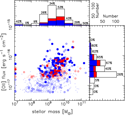
Figure 1: Top: Histograms of [OII] flux measured from narrow-band imaging for all of the NB921 and NB973 [OII] emitters at $z\sim 1.5$ (open) and the emitters targeted in our Subaru/FMOS observations (hatched). Bottom: The distribution of [OII] flux measured from narrow-band imaging as a function of stellar mass for [OII] emitters at $z\sim 1.5$. The NB921 [OII] emitters at $z\approx 1.47$ are shown in blue, while the NB973 [OII] emitters at $z\approx 1.62$ are shown in red. The circles in pale colors show all of the [OII] emitters at $z\sim 1.5$. The large circles show the targeted 313 [OII] emitters in this study. Among them, the filled ones show the 118 [OII] emitters with at least H$\alpha$ or [OIII] detected. The histograms on the right show the distribution of [OII] flux for the targets (open) and the spectroscopically confirmed sample (filled). The numbers signify the percentage of the confirmed galaxies out of the observed ones in each bin of [OII] flux. The histograms on the top show the distribution of stellar mass of the targets and confirmed galaxies. The galaxies for which the stellar masses are poorly estimated are plotted as galaxies with stellar mass of $10^{7}$ .

2.1 Star-forming galaxies at $z\sim 1.5$

2.1.1 Observations

Our samples in the SDF (13h24m38.9s, +27d29m25.9s) contain 933 NB921 [OII] emitters at $z\approx$ 1.450–1.485 with [OII] flux $>$ 5.8 $\times 10^{-18}$ erg s^-1 cm^-2, as well as, 328 NB973 [OII] emitters at $z\approx$ 1.591–1.644 with [OII] flux $>$ 1.7 $\times 10^{-17}$ erg s^-1 cm^-2 (Ly et al., 2007, 2012a). Here, we briefly describe the selection of the [OII] emitters and the measurement of [OII] fluxes. We refer readers to Ly et al. (2007, 2012a) for details. The emission-line galaxies are selected to have a color excess in $z^{\prime}-$NB (NB921 or NB973), where the $z^{\prime}-$NB colors are corrected with $i-z^{\prime}$ color to properly estimate stellar continuum flux at the wavelengths of the NB filters. Then, selections with $BR_{c}i^{\prime}$ and $R_{c}i^{\prime}z^{\prime}$ color-color diagrams are adopted to identify the [OII] emitters at $z\sim 1.47$ or $1.62$. The [OII] fluxes ($F_{\rm[O\emissiontype{II}]}$) are measured as follows:

$$F_{\rm[O\emissiontype{II}]}=\Delta{\rm NB}\frac{f_{\rm NB}-f_{z^{\prime}}}{1-(\Delta{\rm NB}/\Delta z^{\prime})},$$ (1)

where $f_{X}$ and $\Delta{X}$ are the flux density and full width at half maximum (FWHM) of bandpass “$X$”, respectively. The FWHM of $z^{\prime}$ is 955Å.

To detect the six major nebular emission lines in rest-frame optical for these [OII] emitters at $z\sim 1.5$, NIR spectroscopy was conducted with the Fiber Multi Object Spectrograph (FMOS; Kimura et al., 2010) on the Subaru Telescope. FMOS is a unique NIR spectrograph with 400 fibers over a wide field-of-view (FoV), 30 arcmin (diameter). The observations consist of two programs (S12A-026 and S14A-018, PI: M. Hayashi). The first run was carried out on 7–9 April 2012 to observe 313 galaxies at $z\sim 1.5$ (211 NB921 and 102 NB973 [OII] emitters) in high resolution mode in “$H$-long” (1.60–1.80$\mu$m), using three fiber configuration setups. We give a higher priority to galaxies with larger [OII] flux (Figure 1). Six G- or K-type stars with $H=15.5$–17.3 mag are also included in each setup as calibration stars. We use the higher spectral resolution mode ($R\sim 2200$), because it has higher system throughput and is more effective at avoiding contamination from strong OH sky-lines than the low resolution mode ($R\sim 600$). The $H$-band spectra enable us to observe H$\alpha$, [NII]$\lambda$6584, and [SII]$\lambda\lambda$6716,6731. The cross beam switching (CBS) method is adopted, where half of the available fibers are allocated to the targets and, at the same time, the other half of them observe nearby regions of blank sky. That is, a pair of fibers (called “A” and “B”) are allocated to a galaxy, and ABAB dithering is performed for optimal sky subtraction. Observations were only conducted during the last 1.5 nights, because the weather was cloudy for the first one and half nights on 7–9 April. The total integration time was 315, 165, or 150 minutes for 143, 10, or 160 galaxies, respectively. The typical seeing was 0.8–1.0 arcsec in the $R$-band, which was measured for the bright stars near the center of the FoV.

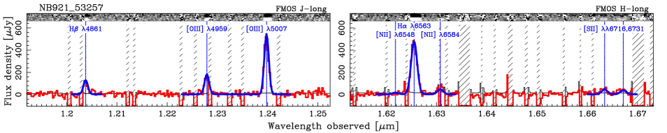
Figure 2: The spectra in $J$- (left) and $H$-band (right) taken with FMOS for one of the brightest [OII] emitters. The red line shows the spectrum of the galaxy, and blue lines show the Gaussian profile fits (§2.1.3). The blue dotted lines show the wavelength of individual emission lines. The black line shows the noise level. The hatched regions show the areas that are masked for strong OH sky lines. The 2-D spectra in A and B fibers are also shown on top. Seven nebular emission lines, H$\beta$, [OIII]$\lambda\lambda$4959,5007, H$\alpha$, [NII]$\lambda$6584, and [SII]$\lambda\lambda$6716,6731, are seen.

The second run was carried out on 11–12 April 2014 to observe 125 galaxies at $z\sim 1.5$ (81 NB921 and 44 NB973 [OII] emitters) in high-resolution mode in “$J$-long” (1.11–1.35$\mu$m) using two fiber configuration setups. The $J$-band spectra enable us to observe H$\beta$ and [OIII]$\lambda\lambda$4959,5007. In the second run, we targeted galaxies observed in the first run for spectral coverage of all emission lines. We gave a higher priority to the galaxies with detections of H$\alpha$ in the $H$-band spectrum. Moreover, since the $J$ and $H$ spectra were taken in different observing conditions on different dates, we allocate fibers to the same calibration stars for accurate flux calibration in all observation runs. The CBS method is also adopted in the second run. On 11 April, almost all of the night was affected by thin cirrus coverage, and the seeing was 0.7–1.1 arcsec. The sky cleared on 12 April, however, the seeing was poor for the first half of the night ($\sim$1.4–1.7 arcsec). Thus, we only obtained optimal data under clear sky condition and sub-arcsec seeing (0.7–1.0 arcsec) for one half-night on 12 April. The total integration time was dependent on the target; 540 (390) minutes for 49 (76) galaxies, respectively. Note that the data taken under marginal conditions are also used in this study after correcting for the loss of flux.

Figure 1 shows the observed [OII] flux of the 313 [OII] emitters targeted in the FMOS observations as a function of stellar mass (§2.1.4). This figure shows that although our target sample is biased toward bright galaxies with $F_{\rm[O\emissiontype{II}]}\gtrsim 5\times 10^{-17}$ erg s^-1 cm^-2, compared with the whole sample of [OII] emitters at $z\sim 1.5$, we have observed star-forming galaxies with stellar mass covering about three orders of magnitude.

2.1.2 Data reduction

The FIBRE-pac data reduction package (Iwamuro et al., 2012) is used to reduce the FMOS data. We run the FIBRE-pac in a standard manner. One difference is that we first reduce the data per each set of succeeding “AB” sequence, and then all of the data are combined after the flux calibration while weighting each frame based on the flux observed through FMOS fibers. Note that the calibration includes the correction for fiber flux loss which is estimated from a calibration star. The effects of differential refraction can be important at high airmasses and with relatively small fibers (1.2” diameter). However, the fiber positioner for FMOS is designed to mitigate these effects (Akiyama et al., 2008). All of the observations were carried out at airmass less than 2.0 and we re-position the fibers every 30 minutes during our observations to account for the different zenith distances. Furthermore, we make sure that the stellar continuum spectrum is well calibrated and there is no discrepancy in the flux between the spectra separated into the $J$-long and $H$-long coverage for the stars used in the flux calibration.

For extended sources, additional aperture correction is required to correct for flux loss. Yabe et al. (2012) have shown that the covering fraction by the 1.2” FMOS fiber is 0.45 for typical galaxies at $z\sim 1.4$. We use the same aperture correction in our galaxies. Note that the covering fraction is not strongly dependent on the size of the point spread function (PSF), if the galaxies are more extended than 1.2”. As mentioned above, the flux calibration by FIBRE-pac corrects for the flux loss for point-sources. The 1.2” aperture includes $\sim$90% of the total flux for the point sources. Here we assume that the FWHM of the PSF is 0.85” and a Gaussian profile for the PSF, since the seeing in the FMOS observations are $\sim$0.8–0.9” in $H$-band. That is, we already corrected for the flux loss by $\sim$10%. Thus, we made aperture corrections of a factor of 2 (=0.9/0.45) for both the $J$- and $H$-band spectra.

Figure 2 shows the $J$- and $H$-band spectra for an individual galaxy that has the largest observed [OII] emission-line flux and all seven nebular emission lines (H$\beta$, [OIII]$\lambda\lambda$4959,5007, H$\alpha$, [NII]$\lambda$6584, and [SII]$\lambda\lambda$6716,6731) are clearly detected.

2.1.3 Line detection

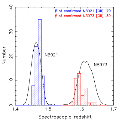
Figure 3: The distribution of redshifts confirmed by FMOS spectroscopy for the 118 [OII] emitters in the SDF. The blue histogram shows the redshift distribution of 79 NB921 [OII] emitters, while the red histogram shows that of 39 NB973 [OII] emitters. The response curves of NB921 and NB973 narrow-band filters are also shown, where the horizontal axis corresponds to the redshift from which [OII] emission is shifted into the narrow-band filter.

We fit Gaussian profiles to the spectra to measure the redshift and the flux of individual emission lines, and estimate the signal-to-noise (S/N) ratio. The Gaussian fitting is conducted separately in the $J$ and $H$ spectra. In each band, major nebular emission lines are simultaneously fitted; H$\beta$ and [OIII]$\lambda\lambda$4959,5007 for $J$-band, and H$\alpha$, [NII]$\lambda$$\lambda$6548,6584, and [SII]$\lambda\lambda$6716,6731 for $H$-band. Note that the width of the Gaussians fits is fixed to the same value of [OIII]$\lambda 5007$ or H$\alpha$. In addition, the flux ratios of the [OIII] and [NII] doublets are fixed to one-third. Each emission line is well fitted with single Gaussian profile with a velocity up to $\sim$100–200 km s^-1 in $\sigma$, i.e., no broad component in the line, suggesting that contamination from Type-1 AGN is negligible. Errors on the emission-line fluxes are estimated using the standard deviation of 500 measurements of the flux, where in each measurement a set of Gaussians is fitted to the spectrum to which the error with normal distribution with 1$\sigma$ spectral noise is added. We regard an emission line with S/N greater than 3 as a detection, and visually inspect it for confirmation.

We succeed in spectroscopically confirming 118 [OII] emitters at $z\sim 1.5$ by detecting some emission lines at more than 3$\sigma$, among which we have detected H$\alpha$ ([OIII]$\lambda$5007) for 115 (45) [OII] emitters. We also have detected H$\beta$, [NII]$\lambda$6584, and [SII]$\lambda\lambda$6716,6731 in 13, 16, and 6 galaxies, respectively. The success rate of line detection is more than 60% for galaxies with observed [OII] flux larger than $\sim 5\times 10^{-17}$ erg s^-1 cm^-2 (Figure 1). The [OIII] and H$\alpha$ emissions are the strongest lines in $J$- and $H$-band spectra, respectively. Even if only a single emission line is detected in the spectrum, it can be identified as being [OIII] or H$\alpha$, because of the additional detection of [OII]$\lambda$3727 from narrow-band imaging. Thus, we can investigate the luminosities of all major nebular emission lines in the rest-frame optical for confirmed galaxies; i.e., [OII], H$\beta$, [OIII], H$\alpha$, [NII], and [SII]. The emission-line fluxes measured for the 118 confirmed galaxies are provided in Table 1.

Spectroscopic redshifts are computed by taking an average of the detected lines. Figure 3 shows the redshift distribution for the 118 galaxies. We note that there is a discrepancy between the peak of the redshift distribution of the [OII] emitters and the response function of the narrow-band filters. The $H$-long observations do not cover wavelengths $\lesssim$1.607$\mu$m in our observations, and also the sensitivity declines sharply at the wavelengths $\gtrsim$1.72$\mu$m. Thus, the H$\alpha$ emission line is hard to detect at $z\lesssim$1.45 and $z\gtrsim$1.62. This is a likely cause for the discrepancy between the redshift distribution and the response of the narrow-band filters. Given an emission-line flux measured with narrow-band imaging, galaxies located further away from the redshift corresponding to the peak of the response curve will have larger intrinsic line fluxes. That is, the redshift distribution shows that H$\alpha$ lines in galaxies with larger intrinsic [OII] flux are likely to be detected. This also suggests that it is important to correct the emission-line flux for the filter response function using spectroscopic redshift to measure the line flux accurately, even if the observed flux is measured with narrow-band imaging.

A fraction of observed galaxies has no emission line detected, which may be due to several reasons. First, as described above, we are likely to miss H$\alpha$ emission lines at $z\lesssim 1.45$ or $z\gtrsim 1.62$. Second, the H$\alpha$ line strength is fainter than the detection limit. This would be the case for targets with observed [OII] flux lower than $\sim 5\times 10^{-17}$ erg s^-1 cm^-2. Indeed, since we regard an emission line at more than 3$\sigma$ as a detection, we find some observed galaxies with marginal detection that are not in excess of 3$\sigma$. Third, the flux of the line is reduced by the masking of OH lines. We note that this is the case for the non-detection of H$\alpha$ or [OIII]$\lambda 5007$ for some galaxies. Finally, it is possible that targeted galaxies are interlopers. However, there are only two instances in NB921 [OII] emitters where the [OII]$\lambda\lambda 3726,3729$ doublet is resolved and detected at $z=3.37$ and 3.72. Thus, we conclude that there is low contamination rate in our samples of [OII] emission-line galaxies at $z\sim 1.5$.

2.1.4 Stellar mass estimates for [OII] emitters

Multi-wavelength data from UV to mid-infrared are available in the SDF. These data allow us to estimate the stellar mass for individual galaxies by fitting the spectral energy distribution (SED) by population synthesis models. Ly et al. (2012a) performed the fitting to the near-UV-to-near-IR SED for the [OII] emitters in this study. Thus, we briefly summarize the procedure of their SED fitting.

We used Bruzual & Charlot (2003) population synthesis models, and assumed the Chabrier (2003) initial mass function (IMF), exponentially declining star formation histories with $\tau$=0.01, 0.1, 1.0, or 10 Gyr, and solar metallicity. Note that the Chabrier (2003) IMF is adopted throughout this paper, although Salpeter (1955) IMF is adopted in Ly et al. (2012a). The assumption in metallicity is justified given gas-phase metallicity measurements of near solar values, as we will demonstrate later (§3.5.2). We also note that the differences in stellar synthesis models are minimal for different metal abundances. The reddening curve of Calzetti et al. (2000) is assumed and dust extinction of $A_{V}$=0.0–3.0 mag is considered.

As shown in Figure 1, the [OII] emitters with emission line detected by FMOS have stellar masses of $3\times 10^{8}$  to $2\times 10^{11}$ . With a range of three orders of magnitude in stellar mass, we are able to study both dwarf and massive star-forming galaxies at $z\sim 1.5$.

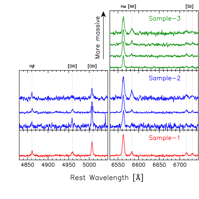
Figure 4: The stacked spectra for the subsamples summarized in Table 2. The sample-1, -2, and -3 are shown in bottom, middle, and top panels, respectively. In each panel, the spectra are shifted vertically for illustration purposes and the dotted lines show the wavelength of individual emission lines. The average stellar mass, $\langle\log(M_{\star}/M_{\odot})\rangle$, of the subsamples increases upward by 1.5 (1.1) dex in the sample-2 (3), respectively. As galaxies are more massive, the [OIII]$\lambda$5007 ([NII]$\lambda$6584) line is weaker (stronger) relative to H$\alpha$.

2.1.5 Stacking FMOS spectra

Since H$\beta$, [NII] and [SII] are generally weak for typical $z\sim 1.5$ galaxies, only one target has all five major nebular lines detected (Figure 2). In many cases, H$\alpha$ line is the only emission line detected, as shown in Tables 1 and 2. Therefore, stacking analyses are essential for investigating the average physical state of ISM in star-forming galaxies at $z\sim 1.5$.

Table 2 summarizes subsamples for stacking. Sample-1 contains all [OII] emitters for which $J$- and $H$-band spectra are available. Sample-2 consists of three subsamples divided by stellar mass. The three subsamples in sample-2 are also selected from all [OII] emitters for which $J$- and $H$-band spectra are available. Sample-3 consists of four subsamples divided by stellar mass, including all [OII] emitters with $H$-band spectra, irrespective of $J$-band data. Sample-3 is used for the analyses involving only H$\alpha$, [NII], and [SII]. The subsamples are defined so that the fraction of the detected emission line is as similar as possible, which avoids a large contribution of a biased number of strong emission lines to the stacked spectra.

To make the stacked spectra, we transform the observed spectra into rest-frame based on the spectroscopic redshift. Then we compute the weighted mean of the spectra based on the noise at each wavelength with 3$\sigma$ clipping. All stacked spectra, shown in Figure 4, detect five nebular emission lines, H$\beta$, [OIII], H$\alpha$, [NII], and [SII]. The line ratios in the individual stacked spectra are shown in Table 3.

2.2 The SDSS data

In order to understand the physical state of ISM in star-forming galaxies at $z\sim 1.5$, comparisons with local galaxies are useful. The local spectroscopic catalogs are extracted from the MPA-JHU release for the Sloan Digital Sky Survey (SDSS) Data Release 7 (DR7) (Kauffmann et al., 2003a; Brinchmann et al., 2004; Salim et al., 2007; Abazajian et al., 2009). We use 86,238 objects that have S/N $\geq 3$ for [OII], H$\beta$, [OIII], H$\alpha$, [NII], and [SII] with stellar mass larger than $10^{8}$at redshifts of 0.04–0.1. These objects are distinguished as star-forming galaxies, AGNs, or galaxies with non-negligible contribution from AGNs (hereafter composite objects) on the Baldwin-Phillips-Terlevich (“BPT”) diagram ([OIII]/H$\beta$ vs. [NII]/H$\alpha$; Baldwin et al. (1981)). The boundary defined by Kewley et al. (2001) is used to discriminate star-forming galaxies and composite objects from AGNs, and then the boundary defined by Kauffmann et al. (2003b) is used to distinguish between star-forming galaxies and composite objects (see also §3.3). The number of star-forming galaxies, composite objects, and AGNs are 67764, 10764, and 7710, respectively.

3 Physical state of ISM in galaxies at $z\sim 1.5$

Six major emission lines in rest-frame optical are available for star-forming galaxies at $z\sim 1.5$ in this study, allowing us to investigate their physical state of ISM in detail. We rely on stacked spectra to study the average properties, since most individual spectra are not deep enough to detect all the nebular emission lines at S/N$>$3. However, we also investigate individual measurements where available.

We first study the electron density of HII regions in $z\sim 1.5$ star-forming galaxies. Electron density has an impact on line strengths. The Balmer lines (e.g., H$\alpha$ and H$\beta$) are emitted from recombination of ionized hydrogen gas, while [OIII] and [OII] are emitted by collisional excitation to forbidden transition states followed by radiative de-excitation. We then correct the emission lines for dust extinction. Correction for dust extinction in the nebular emission is important for reliable measurement of intrinsic ratios of nebular emission lines (e.g., Ly et al., 2012b). Next, we use several line ratios to examine possible contributions of AGN to the emission lines (§3.3), ionization parameter (§3.4), and metal abundance (§3.5). Ionization level is closely related to the intensity of the radiation field in the nebular gas, while metal abundance reflects various galaxy evolution processes. Finally, we investigate the relation between H$\alpha$ and [OII] (§3.6), both of which are widely used as indicators of star formation in galaxies, and the relation between stellar mass and SFR estimated from H$\alpha$ (§3.7). The H$\alpha$ luminosity directly reflects the number of ionizing photons from massive young stars, while the [OII] strength depends in several ways on the physical state of ISM, such as oxygen abundance, ionization parameter, electron temperature, and electron density. However, the use of [OII] has grown in investigating star formation activity in high-$z$ galaxies, since H$\alpha$ redshifts into NIR (MIR) wavebands for galaxies at $z\gtrsim 0.5$ ($z\gtrsim 2.5$).

3.1 Electron density

The intensity ratios of the [OII]$\lambda\lambda$3726,3729 and [SII]$\lambda\lambda$6716,6731 doublets are sensitive to the electron density of ISM. Note that these intensity ratios are independent of dust extinction. Although we have the [OII] luminosity for our full sample, narrow-band imaging does not resolve the [OII] doublet. Instead, we investigate the intensity ratio of the [SII] doublet using the stacked spectra, and individual spectra for bright galaxies.

We find that the galaxies at $z\sim 1.5$ have electron densities ($n_{e}$) of $\sim 10^{2}$ cm^-3. Figure 5 shows that there is no clear dependence of [SII]$\lambda$6716/[SII]$\lambda$6731 on stellar mass of the galaxy, and suggests that electron density in $z\sim 1.5$ star-forming galaxies is consistent with typical estimates for local galaxies, i.e., $n_{e}\sim$10–10² cm^-3 (Osterbrock, 1989; Shirazi et al., 2014). The electron density shown in the right axis of Figure 5 is estimated from the intensity ratio of the [SII] doublet under the assumption of $T_{e}=10^{4}$ K, using the IRAF task temden (Shaw & Dufour, 1994). We also find that [SII]$\lambda$6716/[SII]$\lambda$6731 is not dependent on [OIII]/[OII], suggesting no dependence on the ionization state of ISM (Figure 5). Masters et al. (2014) measure an electron density of $n_{e}\simeq$100–400 cm^-3 for composite spectra of galaxies at $\langle z\rangle=1.85$. Rigby et al. (2011) found an electron density of $n_{e}=252^{+30}_{-28}$ cm^-3 from the ratio of the [OII] doublet in a $z=1.70$ lensed star-forming galaxy. The electron density of our [OII] emitters at $z\sim 1.5$ is consistent with those of galaxies at similar redshifts, and with little evolution as a function of redshift.

Some studies have found higher electron densities of $\sim 10^{3}$ cm^-3 from [SII] doublet measurements for lensed galaxies at $z\sim 2$ (Hainline et al., 2009; Bian et al., 2010). Hainline et al. (2009) derive electron densities of 320–1600 and 1270–2540 cm^-3 for the “Cosmic Horseshoe” ($z=2.38$) and the “Clone” ($z=2.00$), respectively. Bian et al. (2010) measured electron densities of 1029${}^{+3333}_{-669}$ and 1166${}^{+7020}_{-855}$ cm^-3 for two components of J0900+2234, a $z=2.03$ star-forming galaxy. We find that two individual galaxies have [SII] line ratios showing larger electron density of 2.3$\times 10^{3}$ or 8.9$\times 10^{2}$ cm^-3 at $10^{4}$ K. The uncertainties in our individual measurements are large, but our stacks suggest that such galaxies with denser gas are probably not in the majority.

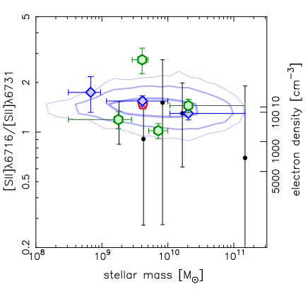
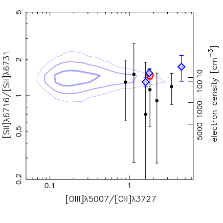
Figure 5: The line ratio of [SII]$\lambda 6716$/[SII]$\lambda 6731$ as a function of stellar mass (top) and [OIII]/[OII] (bottom). The right axis shows the electron density $n_{e}$ corresponding to the line ratio of [SII] doublet at $T_{e}=10^{4}$ K. The black filled circles show the ratio of the individual galaxies with the doublet detected at $>3\sigma$. Red pentagon, blue diamonds, and green hexagons show the average ratios derived from the stacked spectra of sample-1, sample-2 and sample-3, respectively. The contours show the distribution including 68%, 95%, and 99% of star-forming galaxies in the local Universe, where the thicker contour includes the lower percentage of the population.

3.2 Dust extinction

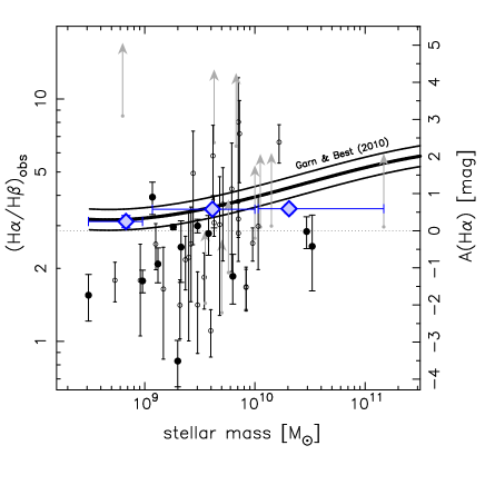
Figure 6: The observed ratio of H$\alpha$ to H$\beta$ (i.e., Balmer decrement), as a function of stellar mass. The right axis shows extinction at 6563Å corresponding to the line ratio of H$\alpha$ to H$\beta$, where the reddening curve of Calzetti et al. (2000) is assumed. The black filled circles show the individual measurements with the two lines detected at $>3\sigma$, while blue squares show the average ratios derived from the stacked spectra (sample-2). The dotted line shows the intrinsic unreddened Case B value of H$\alpha$/H$\beta$=2.86. The stacked spectrum with all galaxies indicates an average line ratio of $\langle$H$\alpha$/H$\beta$$\rangle$=3.57, resulting in $\langle$A(H$\alpha$)$\rangle$=0.63. The open circles show the galaxies with H$\beta$ detected at 2–3$\sigma$, while the arrows show lower limits on the ratio using the 2$\sigma$ upper limit of H$\beta$ for galaxies without H$\beta$ detections. The solid curves show the relation between A(H$\alpha$) and stellar mass in the local Universe and its $\pm 1\sigma$ distribution given by Garn & Best (2010).

The difference between the observed and intrinsic ratios of H$\alpha$ to H$\beta$, i.e., Balmer decrement, can be used to estimate the attenuation of nebular emission by dust. Assuming an electron temperature of $T_{e}=10^{4}$ K and electron density of $n_{e}=10^{2}$ cm^-3 for Case B recombination, the intrinsic ratio of H$\alpha$/H$\beta$ is 2.86 (Osterbrock, 1989). In converting the value of Balmer decrement into extinction at 6563Å, we assume the reddening curve of Calzetti et al. (2000).

Figure 6 shows the observed ratio of H$\alpha$/H$\beta$ as a function of stellar mass. Note that no correction is made for the absorption of stellar continuum at the H$\alpha$ and H$\beta$ wavelengths. The stellar continuum is not detected in individual FMOS spectra, and it is hard to estimate the influence of the absorption of stellar continuum on the Balmer lines reliably with only our data. Thus, we assume that the absorption is weak enough for the correction not to be required, if any (see also, e.g., Steidel et al., 2014).

For individual measurements, about half of them have observed H$\alpha$/H$\beta$ ratios that are consistent with the unreddened Case B value of 2.86 within the uncertainties. However, many galaxies have line ratios of H$\alpha$/H$\beta<$2.86. The reason for the lower line ratio is unclear, however, it is possible that the error is larger than what is shown in the figure, due to the uncertainty in positioning of individual fibers allocated to the galaxies. While assuming a higher electron temperature $T_{e}\gtrsim 10^{4}$ K can slightly reduce the intrinsic H$\alpha$/H$\beta$, the ratio only decreases to 2.74 for $T_{e}=2\times 10^{4}$ K and $n_{e}=10^{2}$ cm^-3 (Osterbrock, 1989). The results of individual dust extinction measurements with both H$\alpha$ and H$\beta$ available can be biased towards relatively low H$\alpha$/H$\beta$ ratios of $\lesssim 2.86$, since H$\beta$ is easier to detect with less dust extinction or intrinsically large H$\beta$ luminosity.

On the other hand, the stacked spectra appear to follow the relation between A(H$\alpha$) and stellar mass given by Garn & Best (2010), although the extinction in the highest mass bin is lower than the relation. As suggested by the dual narrow-band survey simultaneously targeting H$\alpha$ and [OII] for star-forming galaxies at $z\approx 1.47$ (Sobral et al., 2012), we also confirm that the relation of Garn & Best (2010) is applicable to most star-forming galaxies at $z\sim 1.5$ using the Balmer decrement (see also Domínguez et al., 2013; Price et al., 2014). With the stacked spectrum of sample-1, we find that our [OII] emitters have an average dust extinction of $\langle$A(H$\alpha$)$\rangle=0.63$.

In this paper, unless otherwise specified, we adopt the following procedure to correct for dust extinction of nebular emission. First, we assume the dust extinction curve given by Calzetti et al. (2000). For galaxies with both H$\alpha$ and H$\beta$ detected at S/N$>$3, the dust extinction is estimated from Balmer decrement. However, if (H$\alpha$/H$\beta$)${}_{\rm obs}<$2.86, we assume zero dust extinction. For galaxies without an observed H$\alpha$/H$\beta$ ratio, the Garn & Best (2010) relation between A(H$\alpha$) and stellar mass is used.

3.3 BPT diagnostics diagram

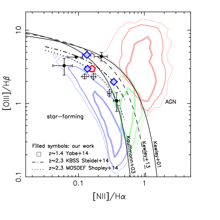
Figure 7: The BPT diagram showing the [OIII]/H$\beta$ ratios versus the [NII]/H$\alpha$ ratio. The black circles show the individual galaxies with all of the four lines detected, while red pentagon and blue diamonds show the average ratios derived from the stacked spectra of sample-1 and sample-2, respectively. Open squares show the line ratios for the stacked spectra of mass-selected star-forming galaxies at $z\sim 1.4$ (Yabe et al., 2014). The dashed-dotted and dotted lines show the relations fitted to $z\sim 2.3$ star-forming galaxies in the Keck Baryonic Structure Survey (KBSS; Steidel et al., 2014) and MOSFIRE Deep Evolution Field (MOSDEF; Shapley et al., 2014) survey, respectively. The contours show the distribution including 68%, 95%, and 99% of star-forming galaxies (blue), composite objects (green), and AGNs (red) in the local Universe, respectively, where the thicker contour includes the lower percentage of the population. The solid lines are the boundaries defined by Kauffmann et al. (2003b) and Kewley et al. (2001) to distinguish the populations at low redshift. The dashed line is the upper limit of the distribution of star-forming galaxies at $z=1.5$ that Kewley et al. (2013b) proposed.

The BPT diagram that compares [OIII]$\lambda$5007/H$\beta$ against [NII]$\lambda$6584/H$\alpha$ (Baldwin et al., 1981) is frequently used to classify galaxies and understand whether massive young stars, shocks, or AGN power the ionization of the gas. We illustrate in Figure 7 the average BPT line ratios, as well as, measurements for individual galaxies if all four lines are detected at S/N$>$3. Here, we apply the boundary defined by Kewley et al. (2001) to identify AGNs, and use Kauffmann et al. (2003b)’s boundary to distinguish star-forming galaxies from composite objects and AGNs. The figure shows that none of our galaxies are located in the AGN region. This result is consistent with the low velocity dispersion of the emission lines, which indicates that our galaxies are not Type-1 AGN (§2.1.3). Since the FMOS fibers measure integrated light, there is still a possibility that the galaxies host an obscured or weak AGN. In such a case, the AGN would not be expected to contribute significantly to the emission lines we observe.

Several recent studies have reported an offset on the BPT diagram for star-forming galaxies at $z\approx 1.5$–2.5, compared with that of local galaxies (e.g., Erb et al., 2006; Rigby et al., 2011; Domínguez et al., 2013; Newman et al., 2014; Shapley et al., 2014; Steidel et al., 2014; Yabe et al., 2014; Zahid et al., 2014). Figure 7 shows that our [OII] emitters at $z\sim 1.5$ also have an offset on the BPT diagram, which is consistent with previous studies. From a photoionization modeling perspective, Kewley et al. (2013b) derive a redshift-dependent boundary to separate purely star-forming galaxies from galaxies hosting an AGN. The revised boundary classifies our [OII] emitters at $z\sim 1.5$ as star-forming galaxies (Figure 7).

Kewley et al. (2013a) discusses the influence of the ionization parameter, the electron density, and the shape of UV spectrum on the BPT line ratios. Kewley et al. (2013a) finds that a higher electron density and a steeper UV spectral slope can result in both BPT line ratios being larger. A higher ionization parameter leads to an upward shift in [OIII]/H$\beta$ in the range of [NII]/H$\alpha$ that our $z\sim 1.5$ [OII] emitters span.

It is an interesting question whether the offset in the BPT diagram is in [NII]/H$\alpha$ or [OIII]/H$\beta$. We attribute most of this “BPT offset” to a higher [OIII]/H$\beta$ ratio at $z\sim 1.5$ than in the local Universe. This is because at a given stellar mass, our [OII] emitters have [NII]/H$\alpha$ ratios that are similar to or slightly smaller than that of local galaxies (§3.5 and see also Stott et al., 2013; Yabe et al., 2014; Zahid et al., 2014). This implies that an upward shift of the [OIII]/H$\beta$ ratio is necessarily required to match the distribution of the local galaxies with that of the [OII] emitters at $z\sim 1.5$, at a given stellar mass. Furthermore, the absence of strong cosmic evolution in the typical line ratio of the [SII] doublet suggests that electron density is not responsible for the BPT offset, as shown in §3.1. One possible explanation is a larger ionization parameter. In the next section, we investigate the ionization parameter for the [OII] emitters at $z\sim 1.5$, and discuss whether this interpretation is correct.

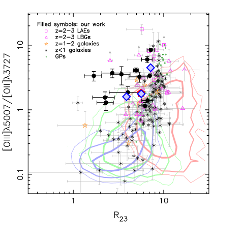
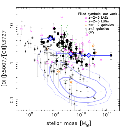
Figure 8: The line ratio of [OIII]/[OII], which is sensitive to ionization parameter, as a function of $R_{23}$ (left) and stellar mass (right). The black circles show the ratio of the individual galaxies with all of the required lines detected, while red pentagon and blue diamonds show the average ratios derived from the stacked spectra of sample-1 and sample-2, respectively. Different populations up to $z\sim 3$ are also shown; LAEs at $z=$2–3 (open squares: Fosbury et al., 2003; Erb et al., 2010; Christensen et al., 2012b; Nakajima et al., 2013), LBGs at $z=$2–3 (open triangles: Pettini et al., 2001; Maiolino et al., 2008; Mannucci et al., 2009; Richard et al., 2011; Wuyts et al., 2012; Belli et al., 2013), star-forming galaxies at $z=$1–2 (open stars: Queyrel et al., 2009; Rigby et al., 2011; Christensen et al., 2012b), star-forming galaxies at $z<1$ (asterisks: Savaglio et al., 2005; Maier et al., 2005; Henry et al., 2013a; Ly et al., 2014a, b), and GPs (open circles: Cardamone et al., 2009). The contours show the distribution including 68%, 95%, and 99% of star-forming galaxies (blue), composite objects (green), and AGNs (red) in the local Universe, respectively, where the thicker contour includes the lower percentage of the population.

3.4 Ionization parameter

It is known that some galaxies at low redshifts, so-called “Green Peas” (GPs; Cardamone et al., 2009), have extremely high [OIII] equivalent width. These green peas are rare, low-mass systems with low metallicity (Cardamone et al., 2009; Amorín et al., 2010). Recent studies have found high-$z$ galaxies that possess strong [OIII] emission (Ly et al., 2007, 2014a, 2014b; van der Wel et al., 2011; Nakajima et al., 2013; Nakajima & Ouchi, 2014; Richardson et al., 2013; Atek et al., 2014; Amorín et al., 2014b; Holden et al., 2014; Shirazi et al., 2014). The ratios of nebular emission lines of star-forming galaxies at $z$=1–3 on the BPT diagram imply that typical galaxies at high redshifts tend to have stronger [OIII] emission, than local star-forming galaxies (Figure 7).

The ionization parameter is defined as

$$q\equiv\frac{Q_{H^{0}}}{4\pi R_{s}^{2}n_{H}},$$ (2)

where $Q_{H^{0}}$ is the number of ionizing photons above the Lyman limit per unit time, $R_{s}$ is the Str$\ddot{\rm o}$mgren radius, and $n_{H}$ is the hydrogen density. The ratio of [OIII]$\lambda$5007 to [OII]$\lambda$3727 is sensitive to the ionization parameter of the ISM (McGaugh, 1991; Kobulnicky & Kewley, 2004; Nakajima & Ouchi, 2014). The effective temperature of ionizing sources also affects the [OIII]/[OII] ratio, since a harder UV photon can ionize O⁺ (Pérez-Montero & Díaz, 2005).

The left panel of Figure 8 shows the ratio of [OIII]/[OII] against the $R_{23}$ index, ([OII]$\lambda$3727+[OIII]$\lambda\lambda$4959,5007)/H$\beta$, for galaxies with the required line detected. In the local Universe, $\sim 0.1$% of SDSS galaxies have [OIII]/[OII] $>1.0$, and a ratio of [OIII]/[OII] $\gtrsim 3.0$ is seldom seen. Compared with local star-forming galaxies, almost all of our [OII] emitters have higher [OIII]/[OII] ratios of $\gtrsim 1$ at all $R_{23}$ values. The [OIII]/[OII] ratios of our [OII] emitters at $z\sim 1.5$ are larger than those of typical galaxies at $z<1$, and consistent with those of galaxies at $z=1$–2 (Queyrel et al., 2009; Rigby et al., 2011; Christensen et al., 2012b), as well as, Lyman $\alpha$ emitters (LAEs) and Lyman break galaxies (LBGs) at $z\sim$2–3 (Richardson et al., 2013; Amorín et al., 2014b; Nakajima & Ouchi, 2014).

The right panel of Figure 8 shows the dependence of [OIII]/[OII] on stellar mass. The contours and asterisks in the figure suggest that there is a similar dependence of [OIII]/[OII] on stellar mass for galaxies at $z=0.04$–0.1 and for star-forming galaxies at $z<1$ (Henry et al., 2013a; Ly et al., 2014a, b). At a given stellar mass, the [OIII]/[OII] ratios of our [OII] emitters are larger than those of typical galaxies at $z<1$, and consistent with those of most galaxies at $z=1$–2 as well as LBGs at $z\sim$2–3. Massive star-forming galaxies with stellar mass of $\sim 10^{10}$ at $z\sim 1.5$ appear to have [OIII]/[OII] ratios that are similar to less massive star-forming galaxies with stellar mass of $\sim 10^{9}$ in the local Universe.

We measure the ionization parameter, $q$ in units of cm s^-1, from the line intensity ratios of $R_{23}$ and $O_{32}$ ([OIII]$\lambda\lambda 4959,5007$/[OII]$\lambda 3727$), using the equations given in Kobulnicky & Kewley (2004) where the photoionization model of Kewley & Dopita (2002) is used. [OII] emitters at $z\sim 1.5$ have $\langle$$\log(q/{\rm cm\ s^{-1}})$$\rangle$=8.1, while star-forming galaxies in the local Universe have $\langle\log(q/{\rm cm\ s^{-1}})\rangle\sim 7.3$ (e.g., Dopita et al., 2006; Nakajima & Ouchi, 2014). Here, we assume that [OII] emitters follow the high-metallicity branch of the relation between metallicity and $R_{23}$ (see §3.5). Even if the low-metallicity branch is assumed, average ionization parameter of [OII] emitters is $\langle$$\log(q/{\rm cm\ s^{-1}})$$\rangle$=7.7. Thus, we conclude that [OIII]/[OII] ratios of [OII] emitters at $z\sim 1.5$ may be increased by higher ionization parameters. We discuss possible mechanisms causing the high ionization parameter in high-$z$ galaxies in §4.

3.5 Gas-phase metallicity

Gas-phase metallicity derived from electron temperature measurements are considered to be the most reliable. This is because metals aid in the cooling of gas by optically-thin radiation, and thus electron temperature is sensitive to the gas-phase metallicity. However, such measurements are difficult to obtain, because the emission line allowing us to estimate the electron temperature is too weak to be detected for individual galaxies. Therefore, several “strong-line” emission-line diagnostics, which are calibrated with local galaxies, are widely used to derive gas-phase metallicity of high-$z$ galaxies. Here, we will assume that these diagnostics are applicable for high-$z$ galaxies.

However, we must be cautious in interpreting high-$z$ metallicity studies. In particular, the measured ionization parameter appears to evolve with redshift (§3.4). Furthermore, recent studies have examined the nitrogen-to-oxygen abundance (N/O), and find enhancement relative to local galaxies with the same oxygen abundance (Teplitz et al., 2000; Amorín et al., 2010; Masters et al., 2014; Shapley et al., 2014).

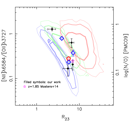
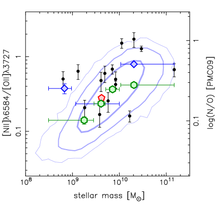
Figure 9: The line ratio of [NII]$\lambda 6584$/[OII]$\lambda 3727$ as a function of $R_{23}$ (top) and stellar mass (bottom). The line ratio is correlated with the nitrogen-to-oxygen ratio (N/O), while $R_{23}$ is an indicator of oxygen abundance, O/H. The black circles show the ratio of the individual galaxies with all of the required lines detected, while the red pentagon, blue diamonds, and green hexagons show the average ratios derived from the stacked spectra of sample-1, sample-2 and sample-3, respectively. The star shows the average ratio for composite spectrum at $\langle z\rangle=1.85$ (Masters et al., 2014). The right axis shows the N/O ratio based on calibration by Pérez-Montero & Contini (2009). The contours show the distribution including 68%, 95%, and 99% of star-forming galaxies (blue), composite objects (green), and AGNs (red) in the local Universe, respectively, where the thicker contour includes the lower percentage of the population.

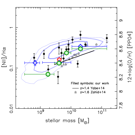
Figure 10: The line ratio of [NII]/H$\alpha$ as a function of stellar mass. The vertical axis on the right shows the oxygen abundance corresponding to the N2 index, using the calibration given by Pettini & Pagel (2004). The black filled circles show the ratio of the individual galaxies with the doublet detected at $>3\sigma$. The red pentagon, blue diamonds, and green hexagons show the average ratios derived from the stacked spectra of sample-1, sample-2 and sample-3, respectively. The solid line and stars show the relations given by Yabe et al. (2014) and Zahid et al. (2014) for star-forming galaxies at $z\sim 1.4$ and $z\sim 1.6$, respectively. The contours show the distribution including 68%, 95%, and 99% of star-forming galaxies in the local Universe, where the thicker contour includes the lower percentage of the population.

3.5.1 N/O abundance ratio

The [NII]$\lambda 6584$/[OII]$\lambda 3727$ ratio is correlated with the nitrogen-to-oxygen abundance ratio in HII regions (Pérez-Montero & Díaz, 2005; Pérez-Montero & Contini, 2009). Since the ionizing potential energies for nitrogen and oxygen are similar, the line intensity ratio is insensitive to ionization conditions (Kewley & Dopita, 2002). The relation between the N/O abundance ratio estimated from the [NII] and [OII] electron temperatures and [NII]$\lambda 6584$/[OII]$\lambda 3727$ is derived by Pérez-Montero & Contini (2009).

Figure 9 shows [NII]$\lambda 6584$/[OII]$\lambda 3727$ as a function of $R_{23}$, that is, the nitrogen-to-oxygen (N/O) ratio as a function of the oxygen abundance (O/H). The distribution of galaxies in the local Universe is overlaid in this figure. At a given oxygen abundance, the [OII] emitters at $z\sim 1.5$ appear to have higher [NII]/[OII] relative to local star-forming galaxies, and the line ratios of the [OII] emitters at $z\sim 1.5$ are similar to those of local composite objects. While local AGNs (red contours) have stronger [NII] emission, compared with star-forming galaxies, the contribution of an AGN in our [OII] emitters is negligible. We made certain that similar results are obtained even if [NII]$\lambda 6584$/[SII]$\lambda\lambda 6716,6731$ is used as a indicator of the N/O abundance ratio (Pérez-Montero & Contini, 2009), instead of [NII]$\lambda 6584$/[OII]$\lambda 3727$.

Given the result that galaxies at $z\sim 1.5$ have higher ionization parameter than local galaxies, the $R_{23}$ value does not necessarily measure metallicity evolution. Higher ionization parameter leads to lower metallicity at a given $R_{23}$ (Kewley & Dopita, 2002), suggesting that oxygen abundance of high-$z$ galaxies is lower than that of local galaxies. Nevertheless, the [OII] emitters at $z\sim 1.5$ are likely to have higher N/O abundance ratio than local star-forming galaxies. The result that we find is similar to recent findings of Amorín et al. (2010) for GPs and Masters et al. (2014) for star-forming galaxies at $z\sim 1.85$. Teplitz et al. (2000) also found high nitrogen abundance for MS 1512-cB58, which is a gravitationally lensed starburst galaxy at $z=2.72$.

Figure 9 also shows that there is no significant difference in dependence of N/O abundance ratio on stellar mass between the [OII] emitters at $z\sim 1.5$ and local star-forming galaxies. This suggests that at a given stellar mass, the [OII] emitters have similar N/O abundance ratio to local star-forming galaxies, which is the same as the recent finding of Amorín et al. (2010) for GPs. On the other hand, Pérez-Montero et al. (2013) found evidence for redshift evolution in the relation between N/O abundance ratio and stellar mass for $z\lesssim 0.4$. In particular, they argue that galaxies at $z=$0.2–0.4 are offset in N/O abundances from local galaxies by -0.14$\pm$0.31 dex. While this is in disagreement with our result for [OII] emitters at $z\sim 1.5$, we note that the selection functions of our sample and Pérez-Montero et al. (2013) are different, and it is not clear if these differences may affect N/O abundance measurements.

Pérez-Montero & Contini (2009) found that it is likely that some star-forming galaxies are classified as composite objects due to high [NII]/H$\alpha$ ratio resulting from high N/O abundance ratio. The SDSS subsample of star-forming galaxies may be biased toward star-forming galaxies with low N/O abundance ratio, which can lead us to underestimate the N/O abundance ratio of local star-forming galaxies. This suggests that it is possible that at a given metallicity the difference in N/O abundance ratio between the [OII] emitters at $z\sim 1.5$ and local star-forming galaxies is smaller than what is shown in Figure 9. Also, this may result in the slight evolution of the relation between N/O abundance ratio and stellar mass, as seen by Pérez-Montero et al. (2013). However, Figure 9 shows that the line ratios of [NII]$\lambda 6584$/[OII]$\lambda 3727$ are similar to those of local composite objects, although in the BPT diagram (Figure 7), most [OII] emitters at $z\sim 1.5$ are located in the star-forming region defined by Kauffmann et al. (2003b). Thus, we cannot completely rule out the possibility that the [OII] emitters at $z\sim 1.5$ have higher N/O abundance ratio at a given metallicity than local star-forming galaxies, while having similar N/O abundance ratio at a given stellar mass. The trends of N/O abundance ratio against oxygen abundance and stellar mass, as shown in Figure 9, appear to be due to the evolution of mass-metallicity relation between the [OII] emitters at $z\sim 1.5$ and local star-forming galaxies.

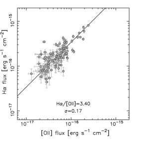
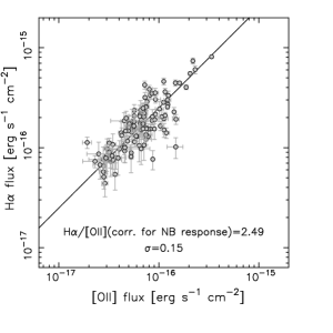
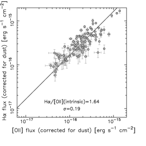
Figure 11: The flux of H$\alpha$ is shown against [OII] flux for [OII] emitters at $z\sim 1.5$. In the left panel, H$\alpha$ flux is not corrected for dust extinction (i.e., observed flux), and [OII] flux is measured from narrow-band imaging (i.e., not corrected for anything). The middle panel is the same as the left one, but for [OII] flux being corrected for the filter response function based on the spectroscopic redshift. In the right panel, H$\alpha$ and [OII] are both corrected for dust extinction (see the text in §3.2 for the details of the procedure of dust correction).

3.5.2 Oxygen abundance from [NII]$\lambda 6584$/H$\alpha$

Figure 10 shows the [NII]$\lambda 6584$/H$\alpha$ ratio as a function of stellar mass. The N2 index, $\log$([NII]$\lambda 6584$/H$\alpha$), is widely used as a proxy for oxygen abundance at high-$z$ (e.g., Denicoló et al., 2002; Pettini & Pagel, 2004). Since different diagnostics can lead to different metallicity estimates (Kewley & Ellison, 2008), one of the merits of using the N2 index is ease of a fair comparison between our result and previous studies (e.g., Erb et al., 2006; Hayashi et al., 2009; Stott et al., 2013; Yabe et al., 2014; Zahid et al., 2014). Figure 10 shows that there is a dependence of the [NII]/H$\alpha$ ratio on stellar mass for both individual galaxies and the average from stacked spectra. The [NII]/H$\alpha$ distribution for individual galaxies at $z\sim 1.5$ is similar to that of local galaxies. We note that individual measurements are biased because of requiring [NII] emission. Thus, the results from stacked spectra (green symbols in the figure) show the proper, average relation for [OII] emitters at $z\sim 1.5$. Our [OII] emitters at $z\sim 1.5$ show steeper increase of the line ratio with the stellar mass, compared to local galaxies. The difference in the [NII]/H$\alpha$ ratio between the two populations is 0.1 dex at the highest stellar mass bin, while the difference is 0.4 dex at the smallest stellar mass bin.

Higher ionization parameter leads to a lower N2 index at a given metallicity (Kewley & Dopita, 2002). With evidence that there is a redshift evolution of the ionization parameter, the difference of the N2 index between various galaxy populations at different redshifts does not necessarily imply a metallicity difference. Since less massive [OII] emitters at $z\sim 1.5$ tend to have higher ionization parameter, the metallicity for less massive galaxies may be more underestimated. We also find that the nitrogen-to-oxygen abundance ratio for [OII] emitters at $z\sim 1.5$ is possibly higher than that of local galaxies, which can lead to overestimating the metallicity (Pérez-Montero & Contini, 2009; Morales-Luis et al., 2014). Thus, all we can conclude from our data is that there is a mass-metallicity relation that extends toward $M_{\star}\sim 10^{9}$  at $z\sim 1.5$.

Photoionization modeling allows us to take into account the dependence of line ratios on the ionization parameter in estimating the metallicity (e.g., McGaugh, 1991; Charlot & Longhetti, 2001; Kewley & Dopita, 2002). The $R_{23}$ index and the relationship between metallicity, ionization parameter, and the line intensity ratios, which is derived from photoionization models, enable estimates of oxygen abundance without the concerns described above (Kobulnicky & Kewley, 2004), although at a given $R_{23}$ value there are two metallicity solutions of low and high metallicities. We will estimate oxygen abundance more reliably with $R_{23}$ index, and then discuss the mass-metallicity relation and the correlation between stellar mass, metallicity, and SFR for our $z\sim 1.5$ [OII] emitters in a forthcoming paper.

3.6 The ratio of H$\alpha$ to [OII]

Hayashi et al. (2013) studied the relation between H$\alpha$ and [OII] for galaxies at $z=1.47$, and concluded that the luminosity of [OII] is well correlated with that of H$\alpha$, and thus [OII] can be used to estimate the star formation activity even at $z=1.47$ (see also Lee et al., 2012; Sobral et al., 2012). However, this study is based on the stacking analysis of narrow-band H$\alpha$ images for [OII] emitters at $z=1.47$. Therefore, it is worth investigating the relation between H$\alpha$ and [OII] for 115 individual galaxies at $z\sim 1.5$.

Figure 11 shows the H$\alpha$ flux as a function of [OII] flux for individual galaxies. The observed fluxes of H$\alpha$ and [OII] are shown in the left panel. There is a clear correlation between H$\alpha$ and [OII] with a low dispersion in the H$\alpha$/[OII] ratio of $\sigma=0.17$. However, as discussed in §2.1.3, the [OII] observed fluxes require corrections for the response function of narrow-band filter. The middle panel demonstrates the importance of the correction, which ranges from 1.0 to 4.7, depending on the redshift of the [OII] emitters (Figure 3). It shows that the correlation between the H$\alpha$ and [OII] observed fluxes is slightly tighter, $\sigma=0.15$. We also investigate the intrinsic ratio of H$\alpha$/[OII] by correcting for dust attenuation (§3.2). The right panel shows again the tight correlation where the ratio is $1.64\pm 0.19$, which is consistent with the line ratio of local galaxies (Kennicutt, 1998; Moustakas et al., 2006) and with $z\sim 2$ H$\alpha$-selected galaxies (Lee et al., 2012). Note that the luminosity range of H$\alpha$ and [OII] covered by individual galaxy samples is different by more than an order of magnitude between at $z\sim 1.5$ and at $z\sim 0$. Nevertheless, the tight correlation between H$\alpha$ and [OII] at $z\sim 1.5$ implies that the [OII] luminosity can be used to estimate star formation activity in galaxies at $z\sim 1.5$, similar to that of local galaxies. This is consistent with the result of Ly et al. (2012a) who compared [OII] and UV SFRs in $z\sim 1.5$ [OII] emitters.

Even if the ratio of H$\alpha$/[OII] is corrected for dust extinction, there is a non-negligible dispersion ($\sigma=0.19$; Figure 11). Since the H$\alpha$/[OII] ratio can depend on the physical conditions in HII regions (e.g., Moustakas et al., 2006; Weiner et al., 2007; Gilbank et al., 2010; Maier et al., 2014b), we compare the ratio to various properties. Figure 12 shows that the H$\alpha$/[OII] ratio depends on stellar mass and the ionization parameter, [OIII]/[OII] (Spearman’s rank correlation coefficient is $\rho=-0.43$ and $\rho=0.61$, respectively), while there seems to be no strong correlation between H$\alpha$/[OII] and [NII]/H$\alpha$, i.e., gas metallicity ($\rho=0.06$). Thus, Figure 12 suggests that less massive galaxies or galaxies with higher ionization parameter tend to have larger H$\alpha$/[OII].

Given the earlier result that less massive galaxies have larger ionization parameter (§3.4), the dependence of H$\alpha$/[OII] on both stellar mass and [OIII]/[OII] appears to be related to the stellar mass–ionization parameter dependence. Since a higher ionization parameter results in a larger O⁺⁺ ionic population relative to O⁺, it is natural to expect a weak [OII] emission for galaxies with high ionization parameter. Indeed, we notice that at a given H$\alpha$ flux, galaxies with larger [OIII]/[OII] ratio tend to have lower [OII] flux. This suggests a dependence of the H$\alpha$/[OII] ratio on the ionization parameter.

The mass-metallicity relation may cause the stellar-mass dependence of H$\alpha$/[OII]. However, the relation between metallicity and $R_{23}$ index (e.g., Pagel et al., 1979) implies that the emission from oxygen ions ([OII] and [OIII]) becomes weaker against Balmer emission (H$\beta$) with increasing metallicity. We here assume that the galaxies follow the high-metallicity branch of the relation between metallicity and $R_{23}$ index. If this is true, the mass-metallicity relation should lead to a positive correlation between H$\alpha$/[OII] and stellar mass, which is contrary to what we observe.

We conclude that although the intrinsic ratio of H$\alpha$/[OII] for star-forming galaxies at $z\sim 1.5$ is consistent with that of local galaxies, the ionization parameter has an impact on the H$\alpha$/[OII] ratio in HII regions.

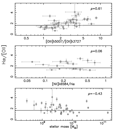
Figure 12: The dust-corrected H$\alpha$/[OII] as a function of stellar mass (bottom), [NII]/H$\alpha$ (middle), and [OIII]/[OII] (top). The solid line shows the H$\alpha$/[OII] ratio of 1.64. The number in the upper right corner of each panel shows Spearman’s rank correlation coefficient. The ratio of [NII]/H$\alpha$ is a proxy of metallicity, while the ratio of [OIII]/[OII] is a proxy of ionization parameter. The ratio of H$\alpha$/[OII] shows a significant dependence on stellar mass and ionization parameter.

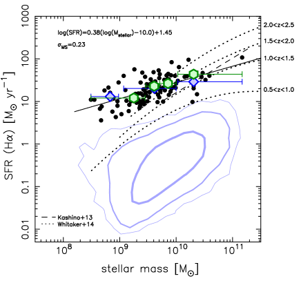
Figure 13: SFR as a function of stellar mass. The SFRs are derived from H$\alpha$ luminosities using the conversion of Kennicutt (1998), with corrections for dust attenuation as discussed in Section 3.2. The black filled circles show the [OII] emitters at $z\sim 1.5$. Blue diamonds, and green hexagons show the average SFRs derived from the stacked spectra of sample-2 and sample-3, respectively. The solid line is derived from a linear fit to the individual [OII] emitters; $\log({\rm SFR})=0.38\times\log(M\star/10^{10}\MO)+1.45$ with a dispersion of 0.23 dex. The contours show the distribution including 68%, 95%, and 99% of star-forming galaxies in the local Universe, where the thicker contour includes the lower percentage of the population. The broken line shows the relation for star-forming galaxies at $z\sim 1.6$ obtained from Subaru/FMOS spectroscopy (Kashino et al., 2013), while the dotted lines are the relations for star-forming galaxies at $z=$0.5–1.0, 1.0–1.5, 1.5–2.0 and 2.0–2.5, respectively (Whitaker et al., 2014).

3.7 Correlation between SFR and stellar mass

It is well known that normal star-forming galaxies at each redshift follow a correlation between SFR and stellar mass from $z\sim 0$ up to $z\sim 3$, which is sometimes called the “main sequence of star formation” or the “star-forming sequence” (e.g., Daddi et al., 2007; Noeske et al., 2007; Salim et al., 2007; Peng et al., 2010; Whitaker et al., 2012, 2014). We investigate the SFRs of the [OII] emitters at $z\sim 1.5$ as a function of stellar mass, where the SFRs are derived from the dust-corrected H$\alpha$ luminosities using the conversion given in Kennicutt (1998). Note that we adjust the conversion factor to that based on Chabrier (2003) IMF to estimate SFRs from H$\alpha$ luminosities. Figure 13 shows that there is a correlation between the SFRs and stellar masses, suggesting that almost all of the [OII] emitters are not extreme galaxies but normal star-forming galaxies which follow the main sequence at their redshift. From fitting a linear function to the individual [OII] emitters, the main sequence (MS) is expressed as $\log({\rm SFR})=0.38\times\log(M_{\star}/10^{10}\MO)+1.45$ with the dispersion of $\sigma_{\rm MS}=0.23$ dex. Such a “main sequence” of star-forming galaxies at $z\sim 1.5$ is consistent with other studies (e.g., Kashino et al., 2013; Whitaker et al., 2014). However, the slope of the relation that we have obtained for the [OII] emitters is shallower than other studies (Figure 13). This seems due to the selection bias for the [OII] emitters with H$\alpha$ emission detected by our NIR spectroscopy.

The local star-forming galaxies are also plotted in Figure 13. Although the [OII] emitters have been demonstrated to be typical star-forming galaxies at $z\sim 1.5$ (see also Ly et al., 2012a), the comparison with the local galaxies indicates that at a given stellar mass, star-forming galaxies at $z\sim 1.5$ have SFRs a factor of $\sim$30 times larger than typical local star-forming galaxies. We discuss the effect of the enhancement of star-forming activity at higher redshifts on the ISM of high-$z$ star-forming galaxies in §4.1.

4 Discussion

Unlike typical local galaxies, we have found that star-forming galaxies at $z\sim 1.5$ have [OIII]/[OII] $\gtrsim 1$ and a large ionization parameter at all stellar masses. We discuss the origin of the large ionization parameter for star-forming galaxies at $z\sim 1.5$, and then compare the line ratios for our star-forming galaxies at $z\sim 1.5$ against several NIR spectroscopic studies of star-forming galaxies at $z\approx$ 1.5–2.5.

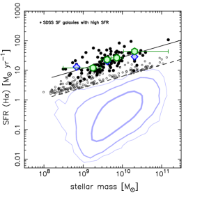
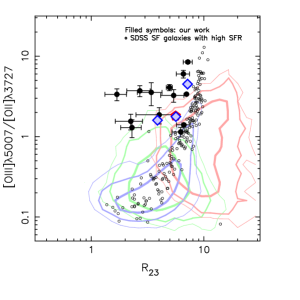
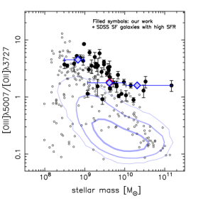
Figure 14: The left panel is the same as Figure 13 and the middle and right panels are the same as Figures 8, but for the SDSS star-forming galaxies with high SFRs comparable to the [OII] emitters at $z\sim 1.5$ also plotted. To compare the line ratios between star-forming galaxies with similar SFRs at $z\sim 0$ and $z\sim 1.5$, SDSS star-forming galaxies meeting the criterion (dashed line in the left panel), $\log({\rm SFR})>0.38\times\log(M_{\star}/10^{10}\MO)+0.8$, are selected (open circles).

4.1 The cause of large ionization parameter

Several mechanisms have been considered to explain the high ionization state (e.g., Pérez-Montero & Díaz, 2005; Kewley et al., 2013a; Nakajima & Ouchi, 2014; Pérez-Montero, 2014): the shape of the ionizing radiation field which depends on an effective temperature of ionizing sources and metallicity, the geometry of nebular gas, and the hydrogen density. Since we find the electron density of HII regions in galaxies at $z\sim 1.5$ is similar to that of local galaxies (§3.1), it is unlikely that there is a significant difference in hydrogen density between star-forming galaxies at $z\sim 0$ and 1.5.

First, we consider the geometry of nebular gas. Equation (2) states that a smaller Str$\ddot{\rm o}$mgren radius can result in a higher ionization parameter. We begin with the simple assumption that the nebular gas has a homogeneous distribution around young stars in HII regions. In an ionization-bounded scenario, the radius of HII regions is the Str$\ddot{\rm o}$mgren sphere radius, which is determined by an equilibrium between photoionization and recombination. In the density-bounded case, the radius is determined by the size of gas clouds, which is smaller than the Str$\ddot{\rm o}$mgren radius. Thus, at a given hydrogen density, density-bounded HII regions are more able to explain high ionization parameters than ionization-bounded regions. We note that the actual distribution of nebular gas is likely to be inhomogeneous. If the distribution of nebular gas within HII regions is clumpy, then a density-bounded scenario is feasible. However, a more detailed discussion on the geometry of nebular gas is not possible with the existing seeing-limited data.

Another possible explanation for the high ionization parameter is due to the radiation field. Of course, AGNs can result in a higher radiation field, and shocks from galactic winds can trigger additional excitation of the ionized gas (e.g., Rich et al., 2011; Fogarty et al., 2012). However, the emission-line ratios and line profiles suggest that an AGN hard radiation field is negligible (Figures 4 and 7). Since lower metallicity, which is found in star-forming galaxies at $z\sim 1.5$, can lead to a harder radiation field, metallicity may play an important role in determining ionization parameter. Indeed, there is a correlation between ionization parameter and metallicity (Pérez-Montero, 2014). However, the left panel of Figure 8 indicates that even at a given $R_{23}$ index (oxygen abundance), star-forming galaxies at $z\sim 1.5$ have larger ionization parameter than galaxies at lower redshifts.

Both SFR and specific SFR (SFR/M_⋆) at a given stellar mass increase with redshift up to $z\sim$ 2–3, and less massive galaxies have higher specific SFRs. (e.g., Whitaker et al., 2012; Speagle et al., 2014; Ilbert et al., 2014; Tasca et al., 2014, and see also Figure 13). Higher star-formation activity corresponds to an increasing number of ionizing photons, which could result in a larger ionization parameter at $z\sim 1.5$ if the geometry and density of gas do not change.

To investigate how the high star-forming activity affects the ionization state of ISM, we compare the [OII] emitters with local star-forming galaxies with comparably large SFRs. They are selected as galaxies with $\log({\rm SFR})>0.38\times\log(M_{\star}/10^{10}\MO)+0.8$ (Figure 14). Only a very small fraction of local galaxies meet this criterion. Figure 14 shows that many local star-forming galaxies with high SFRs are able to have [OIII]/[OII] comparable to the [OII] emitters at $z\sim 1.5$, suggesting that high star-formation activity is important for the high ionization state. However, local star-forming galaxies with high SFRs have a wide range of [OIII]/[OII] ratios, so high star formation activity does not necessarily result in a high ionization state. The middle panel of Figure 14 implies that star-forming galaxies with high [OIII]/[OII] ratios $>1$ have different metallicity at $z\sim 0$ and 1.5. Moreover, at a given stellar mass, there are only a few local galaxies that have high [OIII]/[OII] ratios comparable to the [OII] emitters at $z\sim 1.5$.

As we probe higher redshifts, closer to the formation epoch of the galaxies, the ages of galaxies should be younger. O-type stars (age$<$1–10Myr) as well as Wolf-Rayet stars (age$\sim$3–5Myr) may be present. Also, Stanway et al. (2014) shows that high [OIII]/H$\beta$ ratios with high ionization parameter can be reproduced for up to $\sim$100 Myr by taking into account binary stars, which have a significant impact on the evolution of massive and Wolf-Rayet stars. Therefore, one possibility is that massive young stellar populations harden the radiation field of high-$z$ galaxies.

4.2 Comparison with other high-$z$ galaxies

Stott et al. (2013) studied 193 H$\alpha$ emitters at $z=0.84$ and 1.47, which were selected from the High-redshift Emission Line Survey (HiZELS). The observation was conducted in high resolution mode with Subaru/FMOS. Among the H$\alpha$ emitters, 152 galaxies are at $z=1.47$. Zahid et al. (2014) studied 162 star-forming galaxies at $z\sim 1.6$ in the COSMOS field, which were also observed in high resolution mode with Subaru/FMOS. Among the galaxies with H$\alpha$ detected in $H$-band spectra, 87 galaxies were observed in $J$-band. Yabe et al. (2014) studied 343 star-forming galaxies at $z\sim 1.4$ in the SXDS/UDS field, which were observed in low-resolution mode with Subaru/FMOS. These studies have detected H$\alpha$, H$\beta$, [OIII]$\lambda 5007$, and [NII]$\lambda 6584$ lines for individual galaxies and stacked spectra, and then investigated the line ratios and gas-phase metallicity. The number of galaxies in these studies is a factor of 2–3 larger than our sample. However, our study is the only one with individual intensity measurements of [OII] for 118 galaxies at $z\approx 1.47$ and 1.62.

In terms of BPT diagnostics, we note that our result is consistent with previous high-$z$ studies. Thus, there is a consensus that star-forming galaxies at $z\approx 1.4$–1.6 are offset from local star-forming galaxies with different [OIII]/H$\beta$ and [NII]/H$\alpha$ line ratios (Figure 7).

There is a discrepancy between the stellar mass–[NII]/H$\alpha$ relation that we measure and those of Zahid et al. (2014) and Yabe et al. (2014). At a given stellar mass, star-forming galaxies in our sample show larger [NII]/H$\alpha$ ratios (Figure 10). Note that we convert all stellar mass estimates to a common IMF (Chabrier, 2003), where applicable. Therefore, the reason for the disagreement is unclear. One possibility is a selection bias. Our galaxies are selected by their [OII] emission, while these studies selected by their rest-frame optical continuum ($K_{s}$-selected). Stott et al. (2013) find a higher [NII]/H$\alpha$ ratio as a function of stellar mass. They had selected galaxies by their H$\alpha$ emission. While our result is consistent with that of Stott et al. (2013) at stellar mass $\gtrsim 10^{10}$ , the [NII]/H$\alpha$ ratios of our galaxies are lower at stellar mass $\lesssim 10^{10}$ . Since the sample used in Stott et al. (2013) includes galaxies at $z=0.84$, it may result in higher line ratios, due to the evolving mass–metallicity relation. It is also worth considering whether the ionization parameter and/or N/O abundance are affected by selection effects. However, this investigation requires additional observations, as previous studies do not have information on the [OII] emission.

Large NIR spectroscopic surveys are being conducted at higher redshifts ($z\approx 2.0$–2.6) with Keck/MOSFIRE. Steidel et al. (2014) presented initial results of the Keck Baryonic Structure Survey which studies 179 star-forming galaxies at $z\sim 2.3$. Shapley et al. (2014) presented early observations of the MOSFIRE Deep Evolution Field survey, which studies 118 star-forming galaxies at $z\sim 2.3$. They also show that there is an offset on the BPT diagram from local galaxies (Figure 7 and see also e.g., Erb et al., 2006), and that the N/O abundance ratio of galaxies at $z\sim 2.3$ is likely to be different from local galaxies. Therefore, strong [OIII] emission and high N/O ratio appear to be common in high-$z$ galaxies at $z\approx$ 1.5–2.5.

5 Conclusions

We conducted near-infrared spectroscopy with FMOS on the Subaru Telescope for 118 [OII] emission-line galaxies at $z\sim 1.5$ in the Subaru Deep Field, to investigate the physical state of the interstellar medium of typical star-forming galaxies at high redshift, using rest-frame optical nebular emission lines. The galaxy sample consists of [OII] emitters at $z\approx$1.47 and 1.62 selected by NB921 and NB973 narrow-band imaging with Suprime-Cam on the Subaru Telescope (Ly et al., 2007, 2012a). Moderate-resolution ($R\sim 2200$) spectra in two wavelength regions, 1.11–1.35$\mu$m and 1.60–1.80$\mu$m, were obtained.

We have detected the H$\alpha$ emission line in $H$-band spectra for 115 galaxies, and [OIII]$\lambda$5007 emission line in $J$-band spectra for 45 galaxies. Among these galaxies, H$\beta$, [NII]$\lambda$6584, [SII]$\lambda\lambda$6716,6731 are also detected for 13, 16, and 6 galaxies, respectively. Including the [OII]$\lambda$3727 emission line measured by narrow-band imaging, we use six major nebular emission lines in the rest-frame optical to investigate physical state of the interstellar medium in typical star-forming galaxies at $z\sim$1.5.

We have found a tight correlation between H$\alpha$ and [OII], which suggests that [OII] can be a good indicator of star formation activity for galaxies at $z\sim 1.5$. The line ratios of H$\alpha$/[OII] are consistent with those of local galaxies. We have also found that the H$\alpha$/[OII] line ratio is dependent on ionization parameter and stellar mass. The [OII] emitters suffer dust extinction of $\langle$A(H$\alpha$)$\rangle$=0.63 mag, which is estimated from the H$\alpha$/H$\beta$ Balmer decrement.

We have found that [OII] emitters have strong [OIII] emission. The [OIII]/[OII] ratios are larger than normal star-forming galaxies in the local Universe, suggesting that ionization parameter is enhanced for typical star-forming galaxies at $z\sim 1.5$. Less massive galaxies have larger [OIII]/[OII] ratios. With the result that the electron densities in our galaxies are consistent with local galaxies, the high ionization parameter of galaxies at high redshifts may be attributed to a harder radiation field by young stellar populations and/or the increasing number of ionizing photon from massive stars.

At a given oxygen abundance, star-forming galaxies at $z\sim 1.5$ may have relatively higher nitrogen-to-oxygen abundance ratio, compared to local galaxies. However, no clear difference in N/O abundance ratio is seen between the galaxies at $z\sim 1.5$ and $z\sim 0$ at a given stellar mass. These contrasting results suggest that the evolution of mass-metallicity relation is responsible for the observed trends in N/O abundance ratio at $z\sim 1.5$. The differences in the physical state of the ISM from local galaxies indicate that direct measurements of metallicity, not using diagnostics with strong emission lines which are calibrated with local galaxies, is required to properly study the mass-metallicity relation at high redshifts.

6 Acknowledgments

We thank Enrique P$\acute{\rm e}$rez-Montero for reviewing our manuscript and providing helpful comments, which improved the paper. The data used in this paper were collected at the Subaru Telescope, which is operated by the National Astronomical Observatory of Japan. We thank the Subaru Telescope staff for their invaluable help in assisting our observations. MH acknowledges support from the Japan Society for the Promotion of Science (JSPS) through JSPS Research Fellowship for Young Scientists. CL is funded through the NASA Postdoctoral Program.

Table 1: [OII] emitters in the SDF that are confirmed by Subaru/FMOS spectroscopy.

ID	R.A.	Dec.	$z_{\rm spec}$	[OII]$\lambda$3727	H$\beta$‡	[OIII]$\lambda$5007	H$\alpha$‡	[NII]$\lambda$6584	[SII]$\lambda\lambda$6716,6731
NB921$\_$20415	201.008072	+27.211218	1.465	2.12$\pm$0.05	—	—	2.63$\pm$0.31	$\cdot\cdot\cdot$	$\cdot\cdot\cdot$
NB921$\_$20750	201.080215	+27.211807	1.457	0.72$\pm$0.05	$\cdot\cdot\cdot$	$\cdot\cdot\cdot$	1.14$\pm$0.34	$\cdot\cdot\cdot$	$\cdot\cdot\cdot$
NB921$\_$21503	200.954636	+27.213587	1.465	0.75$\pm$0.05	—	—	1.46$\pm$0.31	$\cdot\cdot\cdot$	$\cdot\cdot\cdot$
NB921$\_$26406	201.117203	+27.227135	1.474	1.32$\pm$0.07	—	—	2.70$\pm$0.80	$\cdot\cdot\cdot$	$\cdot\cdot\cdot$
NB921$\_$28540	201.023178	+27.231798	1.460	0.75$\pm$0.05	—	—	1.63$\pm$0.42	$\cdot\cdot\cdot$	$\cdot\cdot\cdot$
NB921$\_$41594	201.143753	+27.269798	1.464	1.00$\pm$0.04	$\cdot\cdot\cdot$	$\cdot\cdot\cdot$	1.61$\pm$0.28	$\cdot\cdot\cdot$	$\cdot\cdot\cdot$
NB921$\_$42750	201.172729	+27.270859	1.488	1.98$\pm$0.14	—	—	1.88$\pm$0.23	$\cdot\cdot\cdot$	$\cdot\cdot\cdot$
NB921$\_$42929	201.018433	+27.271896	1.464	1.83$\pm$0.05	$\cdot\cdot\cdot$	6.16$\pm$1.61	3.85$\pm$0.21	$\cdot\cdot\cdot$	$\cdot\cdot\cdot$
NB921$\_$49590	201.027985	+27.292707	1.472	2.58$\pm$0.06	—	—	3.87$\pm$0.45	1.24$\pm$0.35	$\cdot\cdot\cdot$
NB921$\_$51600	201.129227	+27.295822	1.469	2.02$\pm$0.05	$\cdot\cdot\cdot$	1.84$\pm$0.34	3.04$\pm$0.28	$\cdot\cdot\cdot$	$\cdot\cdot\cdot$
NB921$\_$52455	201.111649	+27.297915	1.473	1.62$\pm$0.05	$\cdot\cdot\cdot$	6.18$\pm$0.28	2.32$\pm$0.29	$\cdot\cdot\cdot$	$\cdot\cdot\cdot$
NB921$\_$53008	201.323746	+27.299255	1.484	1.27$\pm$0.08	—	—	1.70$\pm$0.10	$\cdot\cdot\cdot$	$\cdot\cdot\cdot$
NB921$\_$53257	200.942825	+27.301119	1.477	3.98$\pm$0.03	3.12$\pm$0.01	13.41$\pm$0.19	8.91$\pm$0.23	0.82$\pm$0.21	0.75$\pm$0.14, 0.63$\pm$0.13
NB921$\_$53590	201.292923	+27.300709	1.462	0.62$\pm$0.04	$\cdot\cdot\cdot$	$\cdot\cdot\cdot$	1.63$\pm$0.18	$\cdot\cdot\cdot$	$\cdot\cdot\cdot$
NB921$\_$53725	200.904846	+27.303421	1.476	4.76$\pm$0.11	$\cdot\cdot\cdot$	$\cdot\cdot\cdot$	3.40$\pm$0.54	$\cdot\cdot\cdot$	$\cdot\cdot\cdot$
NB921$\_$54675	200.977539	+27.304607	1.462	1.25$\pm$0.13	$\cdot\cdot\cdot$	$\cdot\cdot\cdot$	3.27$\pm$0.42	2.15$\pm$0.42	$\cdot\cdot\cdot$
NB921$\_$57905	201.268173	+27.317118	1.481	2.92$\pm$0.10	$\cdot\cdot\cdot$	6.60$\pm$0.90	2.97$\pm$0.30	$\cdot\cdot\cdot$	$\cdot\cdot\cdot$
NB921$\_$59540	200.910477	+27.321886	1.465	1.47$\pm$0.05	$\cdot\cdot\cdot$	$\cdot\cdot\cdot$	1.59$\pm$0.22	$\cdot\cdot\cdot$	$\cdot\cdot\cdot$
NB921$\_$61282	201.276123	+27.327734	1.483	1.12$\pm$0.04	1.53$\pm$0.35	1.73$\pm$0.37	2.84$\pm$0.13	$\cdot\cdot\cdot$	$\cdot\cdot\cdot$
NB921$\_$62719	201.008759	+27.332539	1.466	1.42$\pm$0.05	$\cdot\cdot\cdot$	$\cdot\cdot\cdot$	3.97$\pm$0.56	$\cdot\cdot\cdot$	$\cdot\cdot\cdot$
NB921$\_$63744	200.943481	+27.337433	1.481	5.36$\pm$0.16	2.17$\pm$0.31	6.13$\pm$0.81	6.22$\pm$0.36	$\cdot\cdot\cdot$	$\cdot\cdot\cdot$
NB921$\_$67247	201.047211	+27.349859	1.469	0.53$\pm$0.04	—	—	0.94$\pm$0.20	$\cdot\cdot\cdot$	$\cdot\cdot\cdot$
NB921$\_$68313	200.997437	+27.355768	1.469	1.95$\pm$0.06	$\cdot\cdot\cdot$	$\cdot\cdot\cdot$	1.98$\pm$0.62	$\cdot\cdot\cdot$	$\cdot\cdot\cdot$
NB921$\_$69065	201.120758	+27.358625	1.473	9.15$\pm$0.09	$\cdot\cdot\cdot$	10.40$\pm$0.12	13.20$\pm$1.22	3.88$\pm$0.43	1.71$\pm$0.61, 1.13$\pm$0.36
NB921$\_$72036	201.153427	+27.368980	1.455	1.23$\pm$0.05	$\cdot\cdot\cdot$	$\cdot\cdot\cdot$	2.30$\pm$0.17	$\cdot\cdot\cdot$	$\cdot\cdot\cdot$
NB921$\_$73875	200.918503	+27.376816	1.465	3.95$\pm$0.13	$\cdot\cdot\cdot$	$\cdot\cdot\cdot$	3.75$\pm$0.39	$\cdot\cdot\cdot$	$\cdot\cdot\cdot$
NB921$\_$74041	201.194672	+27.377974	1.456	1.69$\pm$0.05	$\cdot\cdot\cdot$	9.84$\pm$1.60	4.53$\pm$0.27	$\cdot\cdot\cdot$	$\cdot\cdot\cdot$
NB921$\_$74192	201.194168	+27.377691	1.456	0.56$\pm$0.02	1.83$\pm$0.31	1.89$\pm$0.31	1.52$\pm$0.21	$\cdot\cdot\cdot$	$\cdot\cdot\cdot$
NB921$\_$76059	201.091171	+27.385765	1.471	3.37$\pm$0.10	$\cdot\cdot\cdot$	$\cdot\cdot\cdot$	10.16$\pm$0.92	5.11$\pm$0.74	$\cdot\cdot\cdot$
NB921$\_$80256	200.976547	+27.400311	1.465	0.48$\pm$0.03	—	—	1.08$\pm$0.32	$\cdot\cdot\cdot$	$\cdot\cdot\cdot$
NB921$\_$81619	200.982117	+27.405230	1.466	0.46$\pm$0.03	—	—	0.58$\pm$0.15	$\cdot\cdot\cdot$	$\cdot\cdot\cdot$
NB921$\_$84384	201.035858	+27.416105	1.464	2.80$\pm$0.05	1.21$\pm$0.16	3.92$\pm$0.20	3.47$\pm$0.25	$\cdot\cdot\cdot$	$\cdot\cdot\cdot$
NB921$\_$84670	201.296234	+27.416384	1.476	6.12$\pm$0.25	$\cdot\cdot\cdot$	$\cdot\cdot\cdot$	6.31$\pm$1.07	$\cdot\cdot\cdot$	$\cdot\cdot\cdot$
NB921$\_$87249	201.267166	+27.426624	1.456	2.98$\pm$0.08	$\cdot\cdot\cdot$	$\cdot\cdot\cdot$	7.00$\pm$0.53	2.02$\pm$0.28	$\cdot\cdot\cdot$
NB921$\_$87748	201.132797	+27.429152	1.471	3.21$\pm$0.06	$\cdot\cdot\cdot$	5.80$\pm$1.50	6.47$\pm$0.51	1.02$\pm$0.28	1.11$\pm$0.27, 0.99$\pm$0.28
NB921$\_$90789	201.159622	+27.440001	1.487	1.05$\pm$0.08	1.37$\pm$0.07	4.30$\pm$0.20	3.92$\pm$0.16	$\cdot\cdot\cdot$	$\cdot\cdot\cdot$
NB921$\_$90839	200.900070	+27.439596	1.453	0.73$\pm$0.05	$\cdot\cdot\cdot$	$\cdot\cdot\cdot$	1.63$\pm$0.45	$\cdot\cdot\cdot$	$\cdot\cdot\cdot$
NB921$\_$91027	201.097717	+27.441690	1.472	2.33$\pm$0.14	—	—	1.54$\pm$0.46	$\cdot\cdot\cdot$	$\cdot\cdot\cdot$
NB921$\_$91549	201.068466	+27.442301	1.470	2.36$\pm$0.09	$\cdot\cdot\cdot$	$\cdot\cdot\cdot$	4.21$\pm$1.39	$\cdot\cdot\cdot$	$\cdot\cdot\cdot$
NB921$\_$95558	200.978973	+27.457714	1.476	2.66$\pm$0.10	$\cdot\cdot\cdot$	$\cdot\cdot\cdot$	2.24$\pm$0.66	$\cdot\cdot\cdot$	$\cdot\cdot\cdot$
NB921$\_$96152	200.954590	+27.462772	1.477	2.07$\pm$0.08	$\cdot\cdot\cdot$	$\cdot\cdot\cdot$	2.40$\pm$0.33	$\cdot\cdot\cdot$	$\cdot\cdot\cdot$
NB921$\_$97477	201.216415	+27.464403	1.485	0.56$\pm$0.06	0.77$\pm$0.10	3.38$\pm$0.14	1.61$\pm$0.16	0.36$\pm$0.07	$\cdot\cdot\cdot$
NB921$\_$101385	200.912842	+27.481104	1.466	2.19$\pm$0.06	$\cdot\cdot\cdot$	$\cdot\cdot\cdot$	3.34$\pm$0.41	$\cdot\cdot\cdot$	$\cdot\cdot\cdot$
NB921$\_$102638	201.060425	+27.486040	1.472	1.03$\pm$0.05	—	—	2.20$\pm$0.41	$\cdot\cdot\cdot$	$\cdot\cdot\cdot$
NB921$\_$103150	201.024399	+27.487307	1.481	1.20$\pm$0.07	$\cdot\cdot\cdot$	$\cdot\cdot\cdot$	1.74$\pm$0.19	$\cdot\cdot\cdot$	$\cdot\cdot\cdot$
NB921$\_$103705	201.003967	+27.490063	1.475	13.88$\pm$0.48	$\cdot\cdot\cdot$	22.12$\pm$4.73	16.96$\pm$2.02	9.29$\pm$1.81	3.21$\pm$1.09, 4.60$\pm$1.13
NB921$\_$104655	201.087936	+27.493420	1.464	1.22$\pm$0.03	$\cdot\cdot\cdot$	6.37$\pm$0.15	3.40$\pm$0.29	0.61$\pm$0.15	$\cdot\cdot\cdot$
NB921$\_$105983	201.114471	+27.500454	1.485	1.29$\pm$0.10	$\cdot\cdot\cdot$	3.93$\pm$0.31	2.87$\pm$0.39	$\cdot\cdot\cdot$	$\cdot\cdot\cdot$
NB921$\_$107118	201.019028	+27.504000	1.475	1.54$\pm$0.07	$\cdot\cdot\cdot$	$\cdot\cdot\cdot$	3.38$\pm$0.57	$\cdot\cdot\cdot$	$\cdot\cdot\cdot$
NB921$\_$109072	200.994446	+27.512560	1.473	5.21$\pm$0.18	$\cdot\cdot\cdot$	$\cdot\cdot\cdot$	5.93$\pm$0.98	$\cdot\cdot\cdot$	$\cdot\cdot\cdot$
NB921$\_$110460	201.324646	+27.516947	1.476	3.92$\pm$0.12	$\cdot\cdot\cdot$	4.20$\pm$0.85	4.82$\pm$0.86	$\cdot\cdot\cdot$	$\cdot\cdot\cdot$
NB921$\_$110480	201.070343	+27.517275	1.463	1.61$\pm$0.02	1.59$\pm$0.29	5.24$\pm$0.93	4.44$\pm$0.16	0.27$\pm$0.09	$\cdot\cdot\cdot$
NB921$\_$110936	201.257339	+27.518309	1.477	0.51$\pm$0.03	1.12$\pm$0.22	1.88$\pm$0.27	1.73$\pm$0.15	$\cdot\cdot\cdot$	$\cdot\cdot\cdot$
NB921$\_$113063	201.060104	+27.529142	1.475	6.15$\pm$0.18	—	—	2.32$\pm$0.51	$\cdot\cdot\cdot$	$\cdot\cdot\cdot$
NB921$\_$114814	201.170425	+27.533533	1.475	1.55$\pm$0.05	$\cdot\cdot\cdot$	$\cdot\cdot\cdot$	2.37$\pm$0.56	$\cdot\cdot\cdot$	$\cdot\cdot\cdot$
NB921$\_$116328	201.170258	+27.538916	1.476	0.99$\pm$0.04	$\cdot\cdot\cdot$	3.50$\pm$0.18	$\cdot\cdot\cdot$	$\cdot\cdot\cdot$	$\cdot\cdot\cdot$
NB921$\_$116643	201.074005	+27.541149	1.481	1.54$\pm$0.11	$\cdot\cdot\cdot$	$\cdot\cdot\cdot$	3.01$\pm$0.13	$\cdot\cdot\cdot$	$\cdot\cdot\cdot$
NB921$\_$119072	201.065796	+27.551952	1.463	3.40$\pm$0.06	$\cdot\cdot\cdot$	$\cdot\cdot\cdot$	8.64$\pm$0.68	2.03$\pm$0.50	$\cdot\cdot\cdot$
NB921$\_$119235	201.058258	+27.550882	1.473	0.54$\pm$0.04	$\cdot\cdot\cdot$	2.64$\pm$0.26	$\cdot\cdot\cdot$	$\cdot\cdot\cdot$	$\cdot\cdot\cdot$
NB921$\_$119758	201.121780	+27.553385	1.468	1.47$\pm$0.02	2.50$\pm$0.21	12.42$\pm$0.54	4.44$\pm$0.31	$\cdot\cdot\cdot$	$\cdot\cdot\cdot$
NB921$\_$121008	201.245834	+27.557402	1.482	1.38$\pm$0.11	$\cdot\cdot\cdot$	9.59$\pm$0.86	2.63$\pm$0.12	$\cdot\cdot\cdot$	$\cdot\cdot\cdot$
NB921$\_$122309	201.245865	+27.564041	1.461	2.01$\pm$0.08	$\cdot\cdot\cdot$	$\cdot\cdot\cdot$	3.37$\pm$0.49	$\cdot\cdot\cdot$	$\cdot\cdot\cdot$
NB921$\_$126941	201.247879	+27.579729	1.462	1.96$\pm$0.06	$\cdot\cdot\cdot$	$\cdot\cdot\cdot$	4.46$\pm$0.55	$\cdot\cdot\cdot$	$\cdot\cdot\cdot$
NB921$\_$127005	200.998505	+27.580166	1.454	2.29$\pm$0.08	$\cdot\cdot\cdot$	$\cdot\cdot\cdot$	3.40$\pm$0.31	0.58$\pm$0.17	$\cdot\cdot\cdot$
NB921$\_$127149	201.096802	+27.580116	1.478	0.86$\pm$0.07	—	—	1.23$\pm$0.40	$\cdot\cdot\cdot$	$\cdot\cdot\cdot$
NB921$\_$129002	200.981079	+27.589703	1.454	0.77$\pm$0.04	$\cdot\cdot\cdot$	$\cdot\cdot\cdot$	2.61$\pm$0.45	$\cdot\cdot\cdot$	$\cdot\cdot\cdot$
NB921$\_$132078	201.049194	+27.599440	1.475	1.94$\pm$0.07	$\cdot\cdot\cdot$	$\cdot\cdot\cdot$	2.76$\pm$0.57	$\cdot\cdot\cdot$	$\cdot\cdot\cdot$
NB921$\_$133042	201.080048	+27.603086	1.479	0.80$\pm$0.07	$\cdot\cdot\cdot$	$\cdot\cdot\cdot$	1.34$\pm$0.36	$\cdot\cdot\cdot$	$\cdot\cdot\cdot$
NB921$\_$133516	201.124435	+27.609943	1.473	2.20$\pm$0.02	2.60$\pm$0.35	2.84$\pm$0.71	7.38$\pm$0.50	2.80$\pm$0.23	$\cdot\cdot\cdot$
NB921$\_$133703	201.124420	+27.611273	1.476	11.95$\pm$0.15	$\cdot\cdot\cdot$	10.61$\pm$1.02	14.98$\pm$0.60	1.91$\pm$0.32	1.71$\pm$0.30, 1.31$\pm$0.32
NB921$\_$137733	201.037720	+27.619905	1.482	0.43$\pm$0.06	—	—	0.90$\pm$0.25	$\cdot\cdot\cdot$	$\cdot\cdot\cdot$
NB921$\_$139980	201.193390	+27.629015	1.475	0.98$\pm$0.08	—	—	1.56$\pm$0.48	$\cdot\cdot\cdot$	$\cdot\cdot\cdot$
NB921$\_$140463	201.129898	+27.631865	1.478	3.48$\pm$0.08	$\cdot\cdot\cdot$	7.68$\pm$0.18	4.64$\pm$0.28	$\cdot\cdot\cdot$	0.59$\pm$0.21, 0.65$\pm$0.21
NB921$\_$148013	201.166000	+27.658577	1.476	5.18$\pm$0.09	$\cdot\cdot\cdot$	5.41$\pm$0.38	4.75$\pm$0.50	$\cdot\cdot\cdot$	$\cdot\cdot\cdot$
NB921$\_$154909	201.143539	+27.681538	1.475	0.49$\pm$0.04	—	—	0.79$\pm$0.21	$\cdot\cdot\cdot$	$\cdot\cdot\cdot$
NB921$\_$155168	201.056686	+27.683475	1.477	2.00$\pm$0.06	$\cdot\cdot\cdot$	$\cdot\cdot\cdot$	2.42$\pm$0.52	$\cdot\cdot\cdot$	$\cdot\cdot\cdot$
NB921$\_$155600	201.251480	+27.684908	1.479	4.60$\pm$0.11	$\cdot\cdot\cdot$	$\cdot\cdot\cdot$	6.97$\pm$0.76	$\cdot\cdot\cdot$	$\cdot\cdot\cdot$
NB921$\_$159865	201.242142	+27.698488	1.477	1.57$\pm$0.08	$\cdot\cdot\cdot$	$\cdot\cdot\cdot$	1.51$\pm$0.47	$\cdot\cdot\cdot$	$\cdot\cdot\cdot$
NB921$\_$175932	201.045105	+27.753534	1.466	0.48$\pm$0.03	—	—	0.69$\pm$0.17	$\cdot\cdot\cdot$	$\cdot\cdot\cdot$
NB973$\_$39461	201.021744	+27.253485	1.589	2.92$\pm$0.28	$\cdot\cdot\cdot$	$\cdot\cdot\cdot$	3.35$\pm$0.18	$\cdot\cdot\cdot$	$\cdot\cdot\cdot$
NB973$\_$53162	201.155777	+27.293501	1.589	7.87$\pm$0.59	$\cdot\cdot\cdot$	12.54$\pm$0.83	4.96$\pm$0.56	$\cdot\cdot\cdot$	$\cdot\cdot\cdot$
NB973$\_$53375	201.108231	+27.291931	1.595	0.47$\pm$0.13	$\cdot\cdot\cdot$	$\cdot\cdot\cdot$	1.03$\pm$0.34	$\cdot\cdot\cdot$	$\cdot\cdot\cdot$
NB973$\_$53557	200.968735	+27.293095	1.621	0.78$\pm$0.10	$\cdot\cdot\cdot$	3.34$\pm$0.34	1.26$\pm$0.29	$\cdot\cdot\cdot$	$\cdot\cdot\cdot$
NB973$\_$57024	201.082626	+27.301146	1.589	0.86$\pm$0.23	$\cdot\cdot\cdot$	1.32$\pm$0.23	1.49$\pm$0.31	$\cdot\cdot\cdot$	$\cdot\cdot\cdot$
NB973$\_$63423	201.185745	+27.323143	1.590	2.35$\pm$0.33	$\cdot\cdot\cdot$	$\cdot\cdot\cdot$	2.58$\pm$0.53	$\cdot\cdot\cdot$	$\cdot\cdot\cdot$
NB973$\_$63500	201.184814	+27.322449	1.588	2.21$\pm$0.27	—	—	4.97$\pm$0.41	$\cdot\cdot\cdot$	$\cdot\cdot\cdot$
NB973$\_$65046	201.151443	+27.328642	1.599	2.07$\pm$0.25	$\cdot\cdot\cdot$	$\cdot\cdot\cdot$	4.33$\pm$0.57	$\cdot\cdot\cdot$	$\cdot\cdot\cdot$
NB973$\_$65525	201.297684	+27.330811	1.616	0.37$\pm$0.09	—	—	0.96$\pm$0.13	$\cdot\cdot\cdot$	$\cdot\cdot\cdot$
NB973$\_$69720	201.184006	+27.351362	1.616	3.05$\pm$0.24	$\cdot\cdot\cdot$	5.59$\pm$0.49	5.02$\pm$0.43	$\cdot\cdot\cdot$	$\cdot\cdot\cdot$
NB973$\_$71489	200.983398	+27.361053	1.590	4.01$\pm$0.38	$\cdot\cdot\cdot$	$\cdot\cdot\cdot$	4.31$\pm$0.77	$\cdot\cdot\cdot$	$\cdot\cdot\cdot$
NB973$\_$72086	200.994644	+27.363752	1.590	2.11$\pm$0.29	$\cdot\cdot\cdot$	3.04$\pm$0.21	2.19$\pm$0.33	$\cdot\cdot\cdot$	$\cdot\cdot\cdot$
NB973$\_$72650	201.210007	+27.365982	1.600	1.83$\pm$0.14	$\cdot\cdot\cdot$	$\cdot\cdot\cdot$	6.13$\pm$0.56	$\cdot\cdot\cdot$	$\cdot\cdot\cdot$
NB973$\_$72934	201.216019	+27.368015	1.599	5.08$\pm$0.37	$\cdot\cdot\cdot$	$\cdot\cdot\cdot$	5.06$\pm$0.49	$\cdot\cdot\cdot$	$\cdot\cdot\cdot$
NB973$\_$79083	201.158401	+27.401751	1.588	1.56$\pm$0.27	$\cdot\cdot\cdot$	4.29$\pm$0.22	2.53$\pm$0.27	$\cdot\cdot\cdot$	$\cdot\cdot\cdot$
NB973$\_$81424	201.315735	+27.412804	1.591	3.79$\pm$0.31	$\cdot\cdot\cdot$	6.83$\pm$1.01	5.71$\pm$0.90	$\cdot\cdot\cdot$	$\cdot\cdot\cdot$
NB973$\_$85096	200.967087	+27.428595	1.599	0.74$\pm$0.15	—	—	1.23$\pm$0.23	$\cdot\cdot\cdot$	$\cdot\cdot\cdot$
NB973$\_$90084	201.320602	+27.450769	1.591	0.81$\pm$0.21	—	—	1.24$\pm$0.29	$\cdot\cdot\cdot$	$\cdot\cdot\cdot$
NB973$\_$90805	201.290176	+27.456099	1.613	1.93$\pm$0.23	$\cdot\cdot\cdot$	$\cdot\cdot\cdot$	2.54$\pm$0.34	0.96$\pm$0.22	$\cdot\cdot\cdot$
NB973$\_$91278	200.929718	+27.457098	1.597	1.84$\pm$0.20	$\cdot\cdot\cdot$	$\cdot\cdot\cdot$	2.68$\pm$0.34	$\cdot\cdot\cdot$	$\cdot\cdot\cdot$
NB973$\_$91531	201.048340	+27.458298	1.632	0.73$\pm$0.14	$\cdot\cdot\cdot$	3.65$\pm$0.14	$\cdot\cdot\cdot$	$\cdot\cdot\cdot$	$\cdot\cdot\cdot$
NB973$\_$104691	201.186508	+27.529871	1.584	0.92$\pm$0.24	$\cdot\cdot\cdot$	3.51$\pm$0.24	2.39$\pm$0.33	$\cdot\cdot\cdot$	$\cdot\cdot\cdot$
NB973$\_$104719	200.941956	+27.531408	1.617	1.88$\pm$0.06	1.63$\pm$0.56	3.50$\pm$0.80	4.02$\pm$0.21	$\cdot\cdot\cdot$	$\cdot\cdot\cdot$
NB973$\_$105584	201.206970	+27.536465	1.606	2.66$\pm$0.20	$\cdot\cdot\cdot$	6.47$\pm$0.82	5.22$\pm$0.43	$\cdot\cdot\cdot$	$\cdot\cdot\cdot$
NB973$\_$108859	201.048325	+27.549301	1.618	1.84$\pm$0.15	$\cdot\cdot\cdot$	4.71$\pm$0.27	4.15$\pm$0.57	$\cdot\cdot\cdot$	$\cdot\cdot\cdot$
NB973$\_$109063	200.925018	+27.550058	1.616	2.57$\pm$0.22	$\cdot\cdot\cdot$	$\cdot\cdot\cdot$	5.17$\pm$1.25	$\cdot\cdot\cdot$	$\cdot\cdot\cdot$
NB973$\_$109503	200.923508	+27.552755	1.599	2.54$\pm$0.19	$\cdot\cdot\cdot$	7.54$\pm$0.25	6.30$\pm$0.69	$\cdot\cdot\cdot$	$\cdot\cdot\cdot$
NB973$\_$115023	201.158646	+27.577322	1.644	0.45$\pm$0.12	0.76$\pm$0.15	1.60$\pm$0.27	1.86$\pm$0.38	$\cdot\cdot\cdot$	$\cdot\cdot\cdot$
NB973$\_$116135	201.195541	+27.582874	1.589	1.86$\pm$0.31	$\cdot\cdot\cdot$	$\cdot\cdot\cdot$	3.38$\pm$0.73	$\cdot\cdot\cdot$	$\cdot\cdot\cdot$
NB973$\_$117371	201.193390	+27.589464	1.585	1.69$\pm$0.38	—	—	1.66$\pm$0.51	$\cdot\cdot\cdot$	$\cdot\cdot\cdot$
NB973$\_$118086	201.349854	+27.592388	1.596	0.67$\pm$0.14	$\cdot\cdot\cdot$	2.35$\pm$0.38	1.08$\pm$0.30	$\cdot\cdot\cdot$	$\cdot\cdot\cdot$
NB973$\_$123696	200.982178	+27.620754	1.592	3.12$\pm$0.28	$\cdot\cdot\cdot$	$\cdot\cdot\cdot$	4.61$\pm$0.85	$\cdot\cdot\cdot$	$\cdot\cdot\cdot$
NB973$\_$124743	200.944931	+27.624931	1.580	4.44$\pm$0.80	$\cdot\cdot\cdot$	$\cdot\cdot\cdot$	1.90$\pm$0.45	$\cdot\cdot\cdot$	$\cdot\cdot\cdot$
NB973$\_$128025	201.226929	+27.641090	1.610	1.77$\pm$0.22	$\cdot\cdot\cdot$	$\cdot\cdot\cdot$	2.16$\pm$0.64	$\cdot\cdot\cdot$	$\cdot\cdot\cdot$
NB973$\_$128071	201.285156	+27.641356	1.589	1.43$\pm$0.26	—	—	2.15$\pm$0.45	$\cdot\cdot\cdot$	$\cdot\cdot\cdot$
NB973$\_$131961	201.095764	+27.658642	1.585	2.05$\pm$0.38	$\cdot\cdot\cdot$	$\cdot\cdot\cdot$	2.74$\pm$0.46	$\cdot\cdot\cdot$	$\cdot\cdot\cdot$
NB973$\_$133848	201.094513	+27.665018	1.603	0.58$\pm$0.14	$\cdot\cdot\cdot$	$\cdot\cdot\cdot$	1.40$\pm$0.43	$\cdot\cdot\cdot$	$\cdot\cdot\cdot$
NB973$\_$136464	201.200027	+27.675671	1.604	2.19$\pm$0.20	$\cdot\cdot\cdot$	3.66$\pm$0.38	4.13$\pm$1.18	$\cdot\cdot\cdot$	$\cdot\cdot\cdot$
NB973$\_$147549	201.049255	+27.726721	1.598	1.38$\pm$0.17	$\cdot\cdot\cdot$	5.14$\pm$0.78	2.74$\pm$0.34	$\cdot\cdot\cdot$	$\cdot\cdot\cdot$

Note. — Galaxies without $J$-band spectrum available are marked with —, and non-detections are indicated with $\cdot\cdot\cdot$.

Table 2: Subsamples for spectral stacking, which are divided based on stellar mass.

	Coverage	Ntotal	Subsample	N	$\log(M_{\star}/\Mo)$	H$\beta$	[OIII]	H$\alpha$	[NII]	[SII]
sample-1	$J$ and $H$	89		89	9.26 [8.49, 11.2]	13	43	86	14	5
sample-2	$J$ and $H$	89	2a ……	9	8.83 [8.49, 9.00]	2	7	7	1	0
			2b ……	68	9.62 [9.00, 10.0]	9	30	67	8	3
			2c ……	12	10.3 [10.0, 11.2]	2	6	12	5	2
sample-3	$H$	113	3a ……	47	9.25 [8.49, 9.45]	—	—	44	3	1
			3b ……	30	9.46 [9.45, 9.70]	—	—	30	3	1
			3c ……	22	9.85 [9.70, 10.0]	—	—	22	4	1
			3d ……	14	10.3 [10.0, 11.2]	—	—	14	5	2

Note. — The median stellar masses are shown in each subsamples, and the values in brackets are the minimum and maximum of stellar mass in each subsamples. Sample-1 and 2 contain the [OII] emitters that are spectroscopically confirmed and have FMOS spectra in both $J$- and $H$-band. Sample-3 is the same as the others, but the galaxies with FMOS spectra in $H$-band available are all included. The number shown is that of individual emission lines detected in each subsample. Each stacked spectrum is shown in Figure 4.

Table 3: Intensity ratios of emission lines for the stacked spectra of individual subsamples which are summarized in Table 2. All line ratios are corrected for dust extinction, except for H$\alpha$/H$\beta$.

	Subsample	[OIII]/[OII]	[OIII]/H$\beta$	$R_{23}$	H$\alpha$/H$\beta$	[NII]/H$\alpha$	[NII]/[OII]	[SII] doublet
sample-1		1.80$\pm$0.02	2.97$\pm$0.06	5.61$\pm$0.11	3.53$\pm$0.07	0.16$\pm$0.01	0.28$\pm$0.01	1.47$\pm$0.08
sample-2	2a ……	4.49$\pm$0.19	4.61$\pm$0.26	7.17$\pm$0.40	3.12$\pm$0.18	0.13$\pm$0.02	0.37$\pm$0.06	1.74$\pm$0.43
	2b ……	1.77$\pm$0.02	2.98$\pm$0.07	5.65$\pm$0.13	3.51$\pm$0.08	0.14$\pm$0.01	0.23$\pm$0.01	1.54$\pm$0.11
	2c ……	1.60$\pm$0.05	1.98$\pm$0.09	3.88$\pm$0.17	3.53$\pm$0.15	0.34$\pm$0.01	0.79$\pm$0.03	1.30$\pm$0.11
sample-3	3a ……	—	—	—	—	0.07$\pm$0.01	0.14$\pm$0.02	1.19$\pm$0.14
	3b ……	—	—	—	—	0.13$\pm$0.01	0.23$\pm$0.01	2.75$\pm$0.48
	3c ……	—	—	—	—	0.24$\pm$0.01	0.36$\pm$0.01	1.02$\pm$0.11
	3d ……	—	—	—	—	0.30$\pm$0.01	0.42$\pm$0.01	1.45$\pm$0.13

References

- Abazajian et al. (2009) Abazajian, K. N., et al. 2009, ApJS, 182, 543
- Akiyama et al. (2008) Akiyama, M., et al. 2008, Proc. SPIE, 7018, 70182V
- Amorín et al. (2014a) Amorín, R., et al. 2014a, A&A, 568, L8
- Amorín et al. (2014b) —. 2014b, ApJ, 788, L4
- Amorín et al. (2010) Amorín, R. O., Pérez-Montero, E., & Vílchez, J. M. 2010, ApJ, 715, L128
- Atek et al. (2014) Atek, H., et al. 2014, ApJ, 789, 96
- Baldwin et al. (1981) Baldwin, J. A., Phillips, M. M., & Terlevich, R. 1981, PASP, 93, 5
- Belli et al. (2013) Belli, S., Jones, T., Ellis, R. S., & Richard, J. 2013, ApJ, 772, 141
- Bian et al. (2010) Bian, F., et al. 2010, ApJ, 725, 1877
- Brinchmann et al. (2004) Brinchmann, J., Charlot, S., White, S. D. M., Tremonti, C., Kauffmann, G., Heckman, T., & Brinkmann, J. 2004, MNRAS, 351, 1151
- Brinchmann et al. (2008) Brinchmann, J., Pettini, M., & Charlot, S. 2008, MNRAS, 385, 769
- Bruzual & Charlot (2003) Bruzual, G., & Charlot, S. 2003, MNRAS, 344, 1000
- Calzetti et al. (2000) Calzetti, D., Armus, L., Bohlin, R. C., Kinney, A. L., Koornneef, J., & Storchi-Bergmann, T. 2000, ApJ, 533, 682
- Cardamone et al. (2009) Cardamone, C., et al. 2009, MNRAS, 399, 1191
- Chabrier (2003) Chabrier, G. 2003, PASP, 115, 763
- Charlot & Longhetti (2001) Charlot, S., & Longhetti, M. 2001, MNRAS, 323, 887
- Christensen et al. (2012a) Christensen, L., et al. 2012a, MNRAS, 427, 1973
- Christensen et al. (2012b) —. 2012b, MNRAS, 427, 1953
- Daddi et al. (2007) Daddi, E., et al. 2007, ApJ, 670, 156
- de los Reyes et al. (2015) de los Reyes, M. A., et al. 2015, AJ, 149, 79
- Denicoló et al. (2002) Denicoló, G., Terlevich, R., & Terlevich, E. 2002, MNRAS, 330, 69
- Divoy et al. (2014) Divoy, C., et al. 2014, A&A, 569, A64
- Domínguez et al. (2013) Domínguez, A., et al. 2013, ApJ, 763, 145
- Dopita et al. (2006) Dopita, M. A., et al. 2006, ApJ, 647, 244
- Erb et al. (2010) Erb, D. K., Pettini, M., Shapley, A. E., Steidel, C. C., Law, D. R., & Reddy, N. A. 2010, ApJ, 719, 1168
- Erb et al. (2006) Erb, D. K., Shapley, A. E., Pettini, M., Steidel, C. C., Reddy, N. A., & Adelberger, K. L. 2006, ApJ, 644, 813
- Fogarty et al. (2012) Fogarty, L. M. R., et al. 2012, ApJ, 761, 169
- Fosbury et al. (2003) Fosbury, R. A. E., et al. 2003, ApJ, 596, 797
- Garn & Best (2010) Garn, T., & Best, P. N. 2010, MNRAS, 409, 421
- Geach et al. (2011) Geach, J. E., Smail, I., Moran, S. M., MacArthur, L. A., Lagos, C. d. P., & Edge, A. C. 2011, ApJ, 730, L19
- Gilbank et al. (2010) Gilbank, D. G., Baldry, I. K., Balogh, M. L., Glazebrook, K., & Bower, R. G. 2010, MNRAS, 405, 2594
- Hainline et al. (2009) Hainline, K. N., Shapley, A. E., Kornei, K. A., Pettini, M., Buckley-Geer, E., Allam, S. S., & Tucker, D. L. 2009, ApJ, 701, 52
- Hayashi et al. (2013) Hayashi, M., Sobral, D., Best, P. N., Smail, I., & Kodama, T. 2013, MNRAS, 430, 1042
- Hayashi et al. (2009) Hayashi, M., et al. 2009, ApJ, 691, 140
- Henry et al. (2013a) Henry, A., Martin, C. L., Finlator, K., & Dressler, A. 2013a, ApJ, 769, 148
- Henry et al. (2013b) Henry, A., et al. 2013b, ApJ, 776, L27
- Holden et al. (2014) Holden, B. P., et al. 2014, ArXiv:1401.5490
- Hopkins et al. (2007) Hopkins, P. F., Richards, G. T., & Hernquist, L. 2007, ApJ, 654, 731
- Hu et al. (2009) Hu, E. M., Cowie, L. L., Kakazu, Y., & Barger, A. J. 2009, ApJ, 698, 2014
- Ilbert et al. (2014) Ilbert, O., et al. 2014, arXiv:1410.4875
- Iwamuro et al. (2012) Iwamuro, F., et al. 2012, PASJ, 64, 59
- Kakazu et al. (2007) Kakazu, Y., Cowie, L. L., & Hu, E. M. 2007, ApJ, 668, 853
- Kashikawa et al. (2004) Kashikawa, N., et al. 2004, PASJ, 56, 1011
- Kashino et al. (2013) Kashino, D., et al. 2013, ApJ, 777, L8
- Kauffmann et al. (2003a) Kauffmann, G., et al. 2003a, MNRAS, 341, 33
- Kauffmann et al. (2003b) —. 2003b, MNRAS, 346, 1055
- Kennicutt (1998) Kennicutt, Jr., R. C. 1998, ARA&A, 36, 189
- Kewley & Dopita (2002) Kewley, L. J., & Dopita, M. A. 2002, ApJS, 142, 35
- Kewley et al. (2013a) Kewley, L. J., Dopita, M. A., Leitherer, C., Davé, R., Yuan, T., Allen, M., Groves, B., & Sutherland, R. 2013a, ApJ, 774, 100
- Kewley et al. (2001) Kewley, L. J., Dopita, M. A., Sutherland, R. S., Heisler, C. A., & Trevena, J. 2001, ApJ, 556, 121
- Kewley & Ellison (2008) Kewley, L. J., & Ellison, S. L. 2008, ApJ, 681, 1183
- Kewley et al. (2013b) Kewley, L. J., Maier, C., Yabe, K., Ohta, K., Akiyama, M., Dopita, M. A., & Yuan, T. 2013b, ApJ, 774, L10
- Kimura et al. (2010) Kimura, M., et al. 2010, PASJ, 62, 1135
- Kobulnicky & Kewley (2004) Kobulnicky, H. A., & Kewley, L. J. 2004, ApJ, 617, 240
- Lee et al. (2012) Lee, J. C., et al. 2012, PASP, 124, 782
- Leroy et al. (2008) Leroy, A. K., Walter, F., Brinks, E., Bigiel, F., de Blok, W. J. G., Madore, B., & Thornley, M. D. 2008, AJ, 136, 2782
- Liu et al. (2008) Liu, X., Shapley, A. E., Coil, A. L., Brinchmann, J., & Ma, C. 2008, ApJ, 678, 758
- Ly et al. (2011) Ly, C., Lee, J. C., Dale, D. A., Momcheva, I., Salim, S., Staudaher, S., Moore, C. A., & Finn, R. 2011, ApJ, 726, 109
- Ly et al. (2012a) Ly, C., Malkan, M. A., Kashikawa, N., Hayashi, M., Nagao, T., Shimasaku, K., Ota, K., & Ross, N. R. 2012a, ApJ, 757, 63
- Ly et al. (2012b) Ly, C., Malkan, M. A., Kashikawa, N., Ota, K., Shimasaku, K., Iye, M., & Currie, T. 2012b, ApJ, 747, L16
- Ly et al. (2014a) Ly, C., Malkan, M. A., Nagao, T., Kashikawa, N., Shimasaku, K., & Hayashi, M. 2014a, ApJ, 780, 122
- Ly et al. (2014b) Ly, C., Rigby, J., Cooper, M., & Yan, R. 2014b, arXiv: 1412.1834
- Ly et al. (2007) Ly, C., et al. 2007, ApJ, 657, 738
- Maier et al. (2005) Maier, C., Lilly, S. J., Carollo, C. M., Stockton, A., & Brodwin, M. 2005, ApJ, 634, 849
- Maier et al. (2014a) Maier, C., Lilly, S. J., Ziegler, B. L., Contini, T., Pérez Montero, E., Peng, Y., & Balestra, I. 2014a, ApJ, 792, 3
- Maier et al. (2014b) Maier, C., Ziegler, B. L., Lilly, S. J., Contini, T., Perez Montero, E., Lamareille, F., Bolzonella, M., & Le Floc’h, E. 2014b, ArXiv:1410.7389
- Maiolino et al. (2008) Maiolino, R., et al. 2008, A&A, 488, 463
- Mannucci et al. (2009) Mannucci, F., et al. 2009, MNRAS, 398, 1915
- Masters et al. (2014) Masters, D., et al. 2014, ApJ, 785, 153
- McGaugh (1991) McGaugh, S. S. 1991, ApJ, 380, 140
- Miyazaki et al. (2002) Miyazaki, S., et al. 2002, PASJ, 54, 833
- Morales-Luis et al. (2014) Morales-Luis, A. B., Pérez-Montero, E., Sánchez Almeida, J., & Muñoz-Tuñón, C. 2014, ApJ, 797, 81
- Moustakas et al. (2006) Moustakas, J., Kennicutt, Jr., R. C., & Tremonti, C. A. 2006, ApJ, 642, 775
- Nagao et al. (2006) Nagao, T., Maiolino, R., & Marconi, A. 2006, A&A, 459, 85
- Nakajima & Ouchi (2014) Nakajima, K., & Ouchi, M. 2014, MNRAS, 442, 900
- Nakajima et al. (2013) Nakajima, K., Ouchi, M., Shimasaku, K., Hashimoto, T., Ono, Y., & Lee, J. C. 2013, ApJ, 769, 3
- Newman et al. (2014) Newman, S. F., et al. 2014, ApJ, 781, 21
- Noeske et al. (2007) Noeske, K. G., et al. 2007, ApJ, 660, L43
- Oke & Gunn (1983) Oke, J. B., & Gunn, J. E. 1983, ApJ, 266, 713
- Osterbrock (1989) Osterbrock, D. E. 1989, Astrophysics of gaseous nebulae and active galactic nuclei
- Pagel et al. (1979) Pagel, B. E. J., Edmunds, M. G., Blackwell, D. E., Chun, M. S., & Smith, G. 1979, MNRAS, 189, 95
- Peng et al. (2010) Peng, Y.-j., et al. 2010, ApJ, 721, 193
- Pérez-Montero (2014) Pérez-Montero, E. 2014, MNRAS, 441, 2663