$ZZ$ production at high transverse momenta
beyond NLO QCD

Abstract

We study the production of the four-lepton final state $\ell^{+}\ell^{-}\ell^{+}\ell^{-}$, predominantly produced by a pair of electroweak $Z$ bosons, $ZZ$. Using the LoopSim method, we merge NLO QCD results for $ZZ$ and $ZZ$+jet and obtain approximate NNLO predictions for $ZZ$ production. The exact gluon-fusion loop-squared contribution to the $ZZ$ process is also included. On top of that, we add to our merged sample the gluon-fusion $ZZ$+jet contributions from the gluon-gluon channel, which is formally of N³LO and provides approximate results at NLO for the gluon-fusion mechanism. The predictions are obtained with the VBFNLO package and include the leptonic decays of the $Z$ bosons with all off-shell and spin-correlation effects, as well as virtual photon contributions. We compare our predictions with existing results for the total inclusive cross section at NNLO and find a very good agreement. Then, we present results for differential distributions for two experimental setups, one used in searches for anomalous triple gauge boson couplings, the other in Higgs analyses in the four charged-lepton final state channel. We find that the approximate NNLO corrections are large, reaching up to 20% at high transverse momentum of the $Z$ boson or the leading lepton, and are not covered by the NLO scale uncertainties. Distributions of the four-lepton invariant mass are, however, stable with respect to QCD corrections at this order.

1 Introduction

The production of a pair of electroweak vector bosons constitutes an excellent avenue to test the electroweak sector of the Standard Model (SM) at the LHC. This class of processes provides for example information on the non-abelian structure of the Lagrangian. Of particular relevance is the production of a pair of $Z$ bosons, where the underlying gauge structure of $SU(2)_{L}\otimes U(1)_{Y}$ predicts that tri-linear couplings are actually absent at tree-level in the SM. Furthermore, there is a contribution from an $s$-channel Higgs boson resonance, produced in gluon-fusion (GF) via a heavy-quark mediated effective Higgs-gluon coupling. This part allows to perform interference studies and off-shell Higgs width measurements [1, 2, 3, 4, 5, 6].

By the experiments, this process is measured indirectly via $Z$ bosons decaying to a pair of charged leptons or neutrinos each. In this article, we will focus on the four charged-lepton final state

$$pp\rightarrow\ell_{1}^{+}\ell_{1}^{-}\,\ell_{2}^{+}\ell_{2}^{-}+X.$$ (1)

In the past years, the ATLAS and CMS collaborations have provided a rich collection of measurements with increasing accuracy of the four lepton signal, and limits on the trilinear anomalous $ZZ\gamma$ and $ZZZ$ vertices have been deduced [7, 8].

The next-to-leading order (NLO) QCD corrections to $ZZ$ production were first computed in Refs. [9, 10] for on-shell production, and including the leptonic decays and spin correlations in Refs. [11, 12]. They turn out to be sizable, of around 50$\%$, and exhibit a relevant phase-space dependence. In differential distributions, much larger corrections up to the order of 10 can appear. This makes the approximation of correcting the LO differential distribution by the total K-factor (the ratio of the NLO over the LO total cross section), an unreliable estimate of the true NLO differential cross section and can severely underestimate its size. The origin of the large magnitude of the corrections is twofold. At NLO, new partonic sub-processes appear, including those with enhanced gluonic parton distribution functions (PDFs). This explains in part the size of the total K-factor. On the other hand, some new topologies appear for the first time only at NLO. Among them is a topology with a soft or collinear boson emission from a quark or anti-quark, which results in an $\alpha_{s}\alpha_{EW}\ln^{2}(p_{T,j}/m_{V})$ enhancement for a number of observables [13, 14, 15].

The one-loop gluon-induced corrections $gg\to\ell_{1}^{+}\ell_{1}^{-}\,\ell_{2}^{+}\ell_{2}^{-}+X$ are currently known only at LO. They were first reported for on-shell production in Refs. [16, 17]. Results including the leptonic decays  [18, 19] are also available and studies in the framework of Higgs measurements have also been carried out (e.g. Refs. [1, 5, 20, 21]). Formally, they contribute to $ZZ$ production only at next-to-next-to-leading order (NNLO) QCD, but due to the large gluon PDFs at the LHC, their numerical impact is larger than this naive counting of coupling constants suggests. Depending on the selected cuts, their contribution ranges from a few percent up to ten percent. This prediction suffers from large scale uncertainties. However, results at NLO QCD for the gluonic contributions are expected to be available soon – the real corrections, $ZZj$ production, and the virtual two-loop corrections are already known [22, 23].

The NLO electroweak corrections for on-shell $ZZ$ production have been computed in Refs. [24, 25]. They yield only a modest contribution, ranging from the few percent level for integrated cross sections up to 10-20$\%$ for high-$p_{T}$ observables.

At NNLO QCD, further new partonic channels and new topologies contribute. Thus, to match with the expected experimental precision, it is mandatory to assess the size of these NNLO corrections, not only at the total cross section level, but also for the differential distributions. $ZZj$ production at NLO QCD provides the mixed real-virtual and the double real ${\cal O}(\alpha_{s}^{2})$ contributions to the NNLO results. They were first computed in Ref. [26] for on-shell production and account for the new sub-processes and the new topologies appearing for the first time at NNLO. Thus, they are expected to provide the dominant contribution to the total NNLO prediction for selected observables.

The NLO QCD corrections to the double real-emission process, $pp\to\ell_{1}^{+}\ell_{1}^{-}\,\ell_{2}^{+}\ell_{2}^{-}\,jj+X$ have been reported recently [27] with corrections around 10$\%$. The size of the corrections is relatively mild, if adequate central scales are chosen, due to the absence of new channels and phase-space regions opening up at this order, although the uncertainty from varying the factorization and renormalization scale gets greatly reduced.

The two-loop virtual corrections for off-shell $ZZ$ production have been presented in several publications [28, 29, 30, 31] and the NNLO QCD result for the inclusive total cross section has been reported recently [32]. The size of the NNLO corrections compared to the NLO result is about 10%. Up to date, no fully differential NNLO predictions are available in the literature.

In this article, we employ the LoopSim method [13, 33] together with the NLO predictions for $ZZ$ and $ZZj$ production and the LO ones for GF-$ZZ$ and GF-$ZZj$, calculated by the Monte Carlo program VBFNLO [34, 35, 36]. From this procedure, we obtain merged samples that, in certain regions of phase space, are expected to account for the dominant part of the NNLO QCD corrections to the $ZZ$ production process. The abovementioned procedure has been used recently for other diboson production processes [14, 15], as well as V+jet processes [37], resulting in corrections ranging from 30-100$\%$ for selected distributions. Such sizable corrections should be taken into account in experimental analyses.

The article is organized as follows: In Section 2, the details of the theoretical framework of our calculation are given. In section 3, first, we compare our predictions with the existing ones presented in Ref. [32] for on-shell $Z$ pair production at the integrated cross section level at NNLO. Afterwards, differential distributions are also presented for two set of cuts – in Section 3.2.1, the setup of the ATLAS and CMS experimental analyses on $ZZ$ production has been closely followed, while in Section 3.2.2, Higgs search cuts are imposed, following the CMS analysis of Ref. [38]. Finally, in Section 4, we present our summary and conclusions.

2 Theoretical Framework

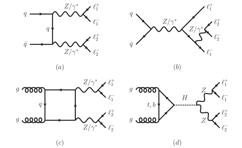
Figure 1: Representative Feynman diagrams for the different production processes contributing to $pp\to\ell_{1}^{+}\ell_{1}^{-}\,\ell_{2}^{+}\ell_{2}^{-}$. Top: $q\bar{q}$ processes appearing at tree-level. Bottom: GF-initiated processes appearing at the one-loop-squared level.

Production of the four-lepton final state happens at leading order mainly via the quark–anti-quark $t/u$-channel diagram (see Fig. 1 $(a)$ for a representative Feynman diagram). The bulk of the contribution comes from on-shell $ZZ$ production, as in that case the electroweak coupling in the $Z$ decay gets effectively replaced by the corresponding branching ratio, which is about $10\%$ for a $Z$ boson decaying into a pair of any charged leptons. Instead of $Z$ bosons, also diagrams appear where these are replaced by virtual photons, denoted as $\gamma^{*}$ in the following. These typically yield lepton pairs with invariant masses much smaller than the $Z$ mass. Their overall contribution strongly depends on the lepton cuts imposed on the final state. Typical experimental invariant mass windows for $Z$ bosons have a lower bound of 66 GeV, which reduces the $\gamma^{*}$ contribution to a negligible level.

Another possibility to produce this four-lepton final state is production of a single vector boson $V\in(Z,\gamma^{*})$, which in turn undergoes a four-body decay into the final-state leptons. An example Feynman diagram is depicted again in Fig. 1 $(b)$. This $s$-channel contribution is also sub-dominant in the SM, since there are no tree-level tri-linear gauge couplings and selection cuts on the final-state leptons suppress these contributions due to the limited phase space to simultaneously produce the two intermediate vector bosons close to their mass shell.

Finally, there are one-loop-squared GF diagrams that can also generate the same four-lepton final-state. These can either proceed via an $s$-channel Higgs resonance, which subsequently decays into $\ell_{1}^{+}\ell_{1}^{-}\,\ell_{2}^{+}\ell_{2}^{-}~{}$and is produced via an effective Higgs-gluon-gluon coupling mediated by loops of heavy-quarks, predominantly the top quark. The dominant contribution to the $H\to\ell_{1}^{+}\ell_{1}^{-}\,\ell_{2}^{+}\ell_{2}^{-}~{}$ decay comes from an intermediate $ZZ^{*}$ system, with one on-shell and one off-shell intermediate vector boson. The other possibility is a continuum production of two, potentially off-shell, $Z/\gamma^{*}$ bosons through a quark-loop box diagram. For typical inclusive cuts, the bulk of the GF contributions originates from on-shell $ZZ$ production, similar to the t/u-channel diagrams. Production via an $s$-channel vector boson resonance is forbidden by gauge invariance and the Landau-Yang theorem [39, 40].

For simplicity, if not stated otherwise, we will refer to the whole process by $ZZ$ production, although we will consider all off-shell effects, non-resonant diagrams and spin correlations of the four-lepton final state. Also, adding the contributions from virtual photons $\gamma^{*}$ is implicitly understood if not mentioned otherwise.

2.1 $\mathbold{ZZ}$ and $\mathbold{ZZj}$ production in VBFNLO

Our calculation relies on the following ingredients. The NLO QCD corrections for the $ZZ$ and the $ZZj$ production processes, as well as the LO one-loop gluon-fusion-induced $gg\to$ $\ell_{1}^{+}\ell_{1}^{-}\,\ell_{2}^{+}\ell_{2}^{-}~{}$and $gg\to$ $\ell_{1}^{+}\ell_{1}^{-}\,\ell_{2}^{+}\ell_{2}^{-}j~{}$contributions are obtained from the VBFNLO package. The NLO QCD corrections to $ZZj$ were included first for this study, and, in the following, we give some details of the methodology used to compute them to make this work self-contained. We follow closely the strategies used for $\ell\nu_{\ell}\gamma\gamma j$ production [41].

We use the spinor-helicity amplitude method and the effective current approach [42, 43] to factorize the electroweak part of the system, containing the leptonic tensor, from the QCD amplitude. We first generate the generic $q\bar{q}\to V_{1}V_{2}j$ amplitudes, where, here and in the following, $V$ denotes either a, possibly virtual, $Z^{(*)}$ boson or a virtual photon $\gamma^{*}$. Additionally, we also calculate the contribution $q\bar{q}\to Vj$. Then the leptonic decays $V_{i}\to\ell_{i}^{+}\ell_{i}^{-}$ and $V\to\ell_{1}^{+}\ell_{1}^{-}\,\ell_{2}^{+}\ell_{2}^{-}~{}$ are attached via effective currents. Note that, in this way, all the off-shell effects and spin correlations are taken into account. All possible flavor and cross-related sub-processes are computed from these generic amplitudes.

At NLO, we need to compute the virtual and the real corrections. To regularize the ultraviolet (UV) and infrared (IR) divergences, we use dimensional regularization [44] and the anti-commuting prescription of $\gamma_{5}$ [45]. We employ the Catani-Seymour algorithm [46] to explicitly cancel the IR divergences prior to the phase-space integration.

To evaluate the scalar integrals, we follow the prescription of Refs. [47, 48, 49] and for the one-loop tensor coefficients, we employ the Passarino-Veltman reduction formalism [50] up to the box level, but avoiding the explicit appearance of Gram determinants [43, 51], and the formalism of Refs. [52, 53], with the notation laid out in Ref. [43] for pentagon integrals.

Several checks have been applied to the virtual amplitudes, computed with the package described in Ref. [43], among them, the factorization of the poles, gauge invariance, and parametrization invariance [43]. For the virtual contributions with closed fermion loops, we set the mass of all the fermions to zero and check that the poles add to zero. Additionally, we have cross-checked both the continuum and Higgs resonance graphs with a second implementation based on FeynArts and FormCalc [54, 55, 56, 57]. On the amplitude level, there are 10-14 digits of agreement for each case. The integrated leading order and real emission contributions have been checked against Sherpa [58] and agreement at the per mille level has been found. Additionally, we have cross-checked that our predictions agree at the per mille level with the ones provided in MCFM [59].

A similar strategy is used for the calculation of $ZZ$ at NLO QCD and the LO gluon fusion $gg\to$ $\ell_{1}^{+}\ell_{1}^{-}\,\ell_{2}^{+}\ell_{2}^{-}~{}$and $gg\to$ $\ell_{1}^{+}\ell_{1}^{-}\,\ell_{2}^{+}\ell_{2}^{-}j~{}$contributions. We include the leptonic decays via effective currents using the spin-helicity formalism and all off-shell effects including Higgs graphs and photons are taken into account. More details on the treatment of the challenging numerical instabilities appearing in $gg\to$ $\ell_{1}^{+}\ell_{1}^{-}\,\ell_{2}^{+}\ell_{2}^{-}j~{}$can be found in Ref. [22].

For the final-state leptons, we consider $Z$ decays into the first two generations, i.e. electrons and muons. We neglect contributions from Pauli interference due to identical particles in the final-state, which is below the per mille level. Therefore, all four possible decay combinations ($V_{1}$, $V_{2}$ decaying into $e$ or $\mu$ each) give the same result and need to be produced only once at the generation level. As we will see later, the cuts are different for same-flavor and different-flavor states, and in the Higgs setup case also for electrons and muons, hence after imposing analysis cuts, the contributions of the four combinations will differ. For the $Z$ resonance, we employ a modified version of the complex-mass scheme [60] where the weak mixing angle is kept real. We work in the five-flavor scheme and use the ${\overline{\text{MS}}}$ renormalization of the strong coupling constant, with the top quark decoupled from the running of $\alpha_{s}$. Diagrams with a final state top quark pair, which would appear in the real emission part of $ZZj$, are considered a separate, experimentally distinguishable process and are therefore discarded. Virtual top-loop contributions in contrast are included in our calculation. We consider a massless bottom-quark, $m_{b}=0$, except for the closed bottom-quark loop amplitudes, where it is set to its pole mass value. The latter is important to correctly account for the negative interference between top- and bottom-quark loops in the effective Higgs-gluon coupling, while for the continuum diagrams the difference between choosing a massless or massive bottom quark is numerically small.

2.2 Computing the dominant part of NNLO with LoopSim

For the calculation of approximate NNLO results for $pp\to$ $\ell_{1}^{+}\ell_{1}^{-}\,\ell_{2}^{+}\ell_{2}^{-}~{}$production, we use the LoopSim method [13, 33]. This approach allows us to merge, in a consistent manner, the $ZZ$@NLO and $ZZj$@NLO samples, provided by VBFNLO, yielding a result which is simultaneously NLO accurate both for the $ZZ$ and $ZZj$ production processes. This merged sample is expected to provide the dominant part of the NNLO QCD correction to $ZZ$ production in phase space regions where additional jet radiation becomes important.

The NLO $ZZj$ predictions provide the double-real and the mixed real-virtual contributions at NNLO of the $ZZ$ result. They are divergent upon integration over the phase space of the real partons and need to be supplemented with double-virtual contributions to yield the finite NNLO result for $ZZ$ production. LoopSim constructs approximate versions of such double-virtual terms by utilizing the fact that their structure of divergences has to match exactly that of the higher multiplicity contributions. This procedure guarantees finiteness of the combined result, while providing a dominant part of the NNLO result for a number of relevant observables. In the process of determining the exact divergent terms of the two-loop corrections, some finite pieces are generated, which are not guaranteed to match the exact constant part of the two-loop diagram. They are, however, proportional to the LO born kinematics and are therefore negligible for distributions which receive sizable corrections at NLO.

To link the two programs, we have made use of an interface [14] which consists, on one hand, of an extension of the VBFNLO program that writes down events in the Les Houches event (LHE) [61] format at NLO and, on the other hand, of a class in the LoopSim library that reads and processes the LHE events.

The LoopSim method proceeds in the following steps. First, an underlying structure for each NLO $ZZj$ event is determined with the help of the Cambridge/Aachen (C/A) [62, 63] algorithm, as implemented in FastJet [64, 65], with a certain radius $R_{\text{LS}}$. This step establishes the sequence of emissions in the input event. For simplicity, we combine each pair of oppositely-charged leptons to a virtual vector boson $V$ and LoopSim processes diagrams at this level. Thereby, we use information from the event generation step to identify the leptons connected by a continuous fermion line. For $s$-channel-type events, which are dominated by contributions where only a single boson is attached to the QCD part of the amplitude, one might consider to also reflect this in the LoopSim part and combine the four leptons into a single particle. The question would then be how to define the transition between the two regions. As this contribution is strongly suppressed by the cuts applied later, we do not pursue this further, but instead always combine the four leptons into two $Z$ bosons. In the next step, the underlying hard structure of the event is determined by working through the $ij\to k$ recombinations in order of decreasing hardness, defined by the $k_{t}$ algorithm measure [66, 67]. The first $n_{b}$ particles associated with the hardest merging are marked as “Born”. The number of Born particles is fixed by the number of outgoing particles in the LO event and is equal to two for the case of $ZZ$ production. At NNLO, the Born particles can be either both vector bosons, a boson and a parton, or two partons. The remaining particles, which are not marked as “Born”, are then “looped” by finding all possible ways of recombining them with the emitters. This step generates approximate one- and two-loop diagrams.

In the next step, a double counting between the approximate one-loop events generated by LoopSim and the exact one-loop events coming from the NLO sample with lower multiplicity is removed. This is done by generating the one-loop diagrams from the tree level events first, and then using them to generate all possible one and two-loop events. This set is then subtracted from the full result, which amounts to removing the two-loop diagrams with both loops simulated by LoopSim and leaving only those with one exact and one simulated loop. To satisfy unitarity, these diagrams are assigned a weight equal to the original event times a prefactor $(-1)^{\text{number of loops}}$. This guarantees that the sum of the weights of the LoopSim-generated events is zero [13]. For a fully inclusive observable, the integrated cross section of our approximated NNLO result would be equal to the NLO one (hence the pure $\alpha_{\text{EW}}^{4}\alpha_{s}^{2}$ contributions would vanish). However, in realistic situations, with finite fiducial volumes or in the case of differential distributions, some of the events generated by LoopSim are removed by cuts or reshuffled within histograms, which results in non-vanishing $\alpha_{\text{EW}}^{4}\alpha_{s}^{2}$ correction and that leads to a genuine, approximate NNLO correction.

The jet C/A and $k_{t}$ algorithms mentioned above depend on the radius $R_{\,\mathrm{LS}}$, which is a parameter of the LoopSim method. The smaller the value of $R_{\,\mathrm{LS}}$, the more likely the particles are recombined with the beam, the larger $R_{\,\mathrm{LS}}$, the more likely they are recombined together. The value of $R_{\,\mathrm{LS}}$ is irrelevant for collinear and soft radiation. It affects only the wide angle (or hard) emissions where the mergings between particles $i$ and $j$ compete with mergings with the beam. In our study, we shall use $R_{\,\mathrm{LS}}=1$, and we shall vary it by $\pm 0.5$. The $R_{\,\mathrm{LS}}$ uncertainty will therefore account for the part of the LoopSim method which is related to attributing the emission sequence and the underlying hard structure of the events.

In order to distinguish our predictions with simulated loops from those with exact loop diagrams, we denote the approximate loops by $\bar{n}$, as opposed to N used for the exact ones. With that notation, for processes whose contributions start at tree level like $q{\bar{q}}\to ZZ$, $\bar{n}\text{LO}$ denotes the correction with simulated one-loop diagrams, and $\bar{n}\text{NLO}$ is a result with exact one-loop and simulated two-loop contributions. However, for processes that start contributing only at one-loop, like $gg\to ZZ$, $\bar{n}\text{LO}$ denotes the correction with respect to that first, non-trivial result. Hence, it is formally an N³LO contribution with respect to the full process of $ZZ$ production.

The GF contribution formally first contributes at NNLO, and consequently we also include it in our merged $\bar{n}\text{NLO}$ sample generated with LoopSim. Due to the large gluonic PDFs, this process can contribute relevantly despite the $\alpha_{s}^{2}$ suppression. Hence, and since it is gauge invariant on its own, by now a common approach in the literature is to add this contribution already to the NLO results. We follow this convention, but make the addition explicit by using the label “NLO+LO-GF” in this case. Additionally, as mentioned before, we also merge the real radiation process GF-$ZZj$ computed at LO to the GF-$ZZ$ result, yielding a contribution appearing only at N³LO. Our results will in general also include this contribution, where we label the full results as “$\bar{n}$NLO +$\bar{n}$LO-GF”. In summary, the GF contribution is always implicitely understood to be included at the corresponding order given by the power counting of coupling constants, in particular LO-GF in the $\bar{n}$NLO result. If additional GF contributions are added, this is made explicit in the label.

3 Numerical Results

3.1 Comparison with inclusive NNLO calculation

$\sigma_{\text{LO}}$ [pb]	5.0673(4) ${}^{+1.6\%}_{-2.7\%}$	(Ref. [32]: 5.060 ${}^{+1.6\%}_{-2.7\%}$)
$\sigma_{\text{NLO}}$ [pb]	7.3788(10) ${}^{+2.8\%}_{-2.3\%}$	(Ref. [32]: 7.369 ${}^{+2.8\%}_{-2.3\%}$)
$\sigma_{\text{NLO}+\text{LO-GF}}$ [pb]	7.946(3) ${}^{+4.2\%}_{-3.2\%}$
$\sigma_{\text{NNLO}}$ [pb]		(Ref. [32]: 8.284 ${}^{+3.0\%}_{-2.3\%}$)
$\sigma_{\bar{n}\text{NLO}}$ [pb]	8.103(5) ${}^{+4.7\%}_{-2.6\%}$ $(\mu)$  ${}^{+0.8\%}_{-0.6\%}$ ($R_{LS}$)
$\sigma_{\bar{n}\text{NLO}+\bar{n}\text{LO}\text{-GF}}$ [pb]	8.118(5) ${}^{+4.7\%}_{-2.6\%}$ $(\mu)$  ${}^{+0.8\%}_{-0.6\%}$ ($R_{LS}$)

Table 1: Comparison with Ref. [32] of total cross sections for on-shell $ZZ$ production at the LHC running at $\sqrt{s}=8\,\text{TeV}$. The errors in brackets are the statistical error from Monte Carlo integration, while the percentages give the scale variation error, obtained from changing $\mu_{F}$ and $\mu_{R}$ independently within the range $[\frac{1}{2}m_{Z};2m_{Z}]$, where the ratio $\mu_{F}/\mu_{R}$ is constrained to stay within $[\frac{1}{2};2]$. For the $\bar{n}\text{NLO}$ results we additionally give the error due to a variation of $R_{{\,\mathrm{LS}}}$ between $0.5$ and $1.5$.

We start by comparing the results obtained with LoopSim+VBFNLO with the calculation of the inclusive NNLO cross section of Ref. [32]. Here, in contrast to the rest of the paper, we use the settings as those of Ref. [32], i.e. the $Z$ bosons are on-shell and do not decay, hence no cut is placed on the final state. Also, all numerical values of masses and couplings are taken from there, namely $m_{W}=80.399\,\mathrm{GeV}$, $m_{Z}=91.1876\,\mathrm{GeV}$, $G_{F}=1.16639\times 10^{-5}\,\mathrm{GeV}^{-2}$, $m_{t}=173.2\,\mathrm{GeV}$, $m_{H}=125\,\mathrm{GeV}$ and $\mu_{R}=\mu_{F}=m_{Z}$. As PDFs, the MSTW 2008 set [68] is chosen, evaluated at each corresponding order. Since our matrix elements include all off-shell effects and spin correlations in our prediction of $\ell_{1}^{+}\ell_{1}^{-}\,\ell_{2}^{+}\ell_{2}^{-}~{}$production, for this comparison, we have to modify our code. All the $s$-channel contributions, like the example diagram in Fig. 1 $(b)$, or the $t/u$-channel contributions with $\gamma^{*}$ in the intermediate state are set to zero. Hence, the only contribution comes from $t/u$-channel diagrams of Fig. 1 with on-shell $Z$ bosons. For the GF part, both Higgs and continuum diagrams contribute, but for the latter we also have to remove all diagrams with virtual photons. In the phase-space generator, the (Breit-Wigner) distributions for the invariant mass of the $Z$ bosons are replaced by $\delta$-distributions at the $Z$ pole mass. As leptonic decays of the $Z$ bosons are still simulated internally, we finally need to account for this by dividing the result by $\text{BR}(Z\to\ell_{i}^{+}\ell_{i}^{-})^{2}$. The resulting cross sections at 8 TeV are shown in Table 1.

At LO and NLO, agreement at the per mille level is found. The NLO integrated K-factor, defined as the ratio of NLO/LO predictions, is 1.46. For comparison, we also show the result of adding the GF contribution, formally NNLO, to the NLO result, evaluating both with NNLO PDFs. This is the best currently available estimate without requiring the evaluation of two-loop diagrams or merging different jet multiplicities. We see that these give an additional 7.7% contribution to the NLO cross section, or a total K factor of 1.57 comparing NLO+GF to the LO result. Additionally, they increase the scale variation uncertainty significantly. The latter comes from the fact that the GF contribution is the lowest order accuracy result for the $gg$ channel.

With respect to NLO, the total NNLO correction, computed in Ref. [32] and quoted in the fourth row of Table 1, is about $12\%$. Hence, the GF contribution provides the leading part of those, namely 60%. Our approximate $\bar{n}$NLO and $\bar{n}$NLO +$\bar{n}$LO-GF results are shown in the last two rows of Table 1. Their overall agreement with the full NNLO result is good with the difference at the level of 2$\%$ only. This is not a priori guaranteed by our method and is consistent with the assumption of a LO $\times$ $\alpha_{s}^{2}$ effect coming from the genuine finite pieces of the exact two-loop virtual amplitudes. These terms are not properly determined by our method, but they are covered by the remaining scale uncertainty. The scale uncertainty of our $\bar{n}$NLO result is similar to NLO+GF, and not reduced like for the NNLO result, since the LoopSim method does not attempt to reconstruct higher-order terms proportional to the scale dependence in order not to underestimate the variation, although, technically, this would be possible.

3.2 Differential distributions

In the following sections, results at the LHC at $\sqrt{s}=8$ $\,\mathrm{TeV}$ will be given for two different sets of cuts. In Section 3.2.1, we closely follow the ATLAS and CMS experimental analyses on $ZZ$ production, while in Section 3.2.2, we impose Higgs search cuts, following the CMS analysis of Ref. [38]. Below, we describe the common settings.

As input parameters, we use

$$m_{Z} =91.1876\,\mathrm{GeV}\,, G_{F} =1.16637\times 10^{-5}\,\mathrm{GeV}^{-2}\,,$$

$$m_{W} =80.398\,\mathrm{GeV}\,, \alpha_{\text{em}}^{-1} =132.3407\,,$$

$$m_{H} =125\,\mathrm{GeV}\,, \sin^{2}(\theta_{W}) =0.22265\,,$$ (2)

$$\Gamma_{Z} =2.508\,\mathrm{GeV}\,, \Gamma_{H} =0.004017\,\mathrm{GeV}\,.$$

The mass of the top and bottom quarks, which run in the closed fermion loops, are set to

$$m_{t} =172.4\,\mathrm{GeV}\,, m_{b}=4.855\,\mathrm{GeV}\ .$$ (3)

All other quarks, including external bottom quarks, are taken as massless.

The jets are defined with the anti-$k_{t}$ algorithm [69], as implemented in FastJet [64, 70], with the radius $R=0.4$. Independently of the order of a prediction, we use the NNLO MSTW2008 [68] PDF set, provided by the LHAPDF [71] implementation with $\alpha_{s}(m_{Z})=0.11707$.

At fixed order in perturbation theory, the cross section depends on the renormalization and factorization scale. As central values for both of those scales, we choose the scalar sum of the transverse energy of the system

$$\mu_{F,R}=\mu_{0}=\frac{1}{2}\left(\sum p_{T,\text{partons}}+\sqrt{p_{T,V_{1}}^{2}+m_{V_{1}}^{2}}+\sqrt{p_{T,V_{2}}^{2}+m_{V_{2}}^{2}}\right)\,,$$ (4)

where $p_{T,V_{1,2}}$ and $m_{V_{1,2}}$ are the transverse momenta and invariant masses of the recombined, opposite-signed charged lepton pairs, respectively. The scale uncertainty is obtained by varying simultaneously the factorization and renormalization scale by a factor two around the central scale. Additionally, to assess the uncertainties associated with the recombination method used by LoopSim, we show the uncertainty bands associated with variations of $\pm 0.5$ around $R_{\text{LS}}=1$.

3.2.1 $\mathbold{ZZ}$ analysis

In the analysis of $ZZ$ production, we use the following cuts, inspired largely by the ATLAS paper [7]. The settings of the corresponding CMS analysis [8] are comparable. The transverse momenta and pseudorapidities of leptons, as well as those of jets (for observables exclusive with respect to jet activity), and the distance between leptons and leptons and jets are required to stay in the following fiducial volume:

$$p_{t,\ell} >20\,\mathrm{GeV}\,, |\eta_{\ell}| <2.5\,,$$

$$p_{t,{\,\mathrm{jet}}} >25\,\mathrm{GeV}\,, |\eta_{{\,\mathrm{jet}}}| <4.5\,,$$ (5)

$$\Delta R_{\ell,{\,\mathrm{jet}}} >0.3\,, \Delta R_{\ell,\ell} >0.2\,.$$

To reconstruct the $Z$ bosons from the leptons, we employ the following algorithm. First, all invariant-mass pairs of same-flavor and opposite-sign lepton pairs are formed. If all leptons are of the same generation, there are in total four possibilities, while for different generations only two exist. The invariant-mass pair closest to the physical $Z$ boson mass is labeled $Z_{1}$ and it is required to satisfy the cut $66\,\mathrm{GeV}<m_{\text{inv},Z_{1}}<116\,\mathrm{GeV}$, otherwise the event is discarded. If the second pair of leptons, which we denote as $Z_{2}$, falls into the same mass window, the event is labelled as $ZZ$, if not, it is called a $ZZ^{\star}$ event, provided that $m_{Z_{2}}>20\,\mathrm{GeV}$. If the latter is not satisfied, the event is rejected. Hence, our two selection types can be summarized as

$$\begin{array}[]{lc}ZZ\text{ selection: }&m_{Z_{1}},m_{Z_{2}}\in(66,116)\,\mathrm{GeV}\,,\\ ZZ^{*}\text{ selection: }&m_{Z_{1}}\in(66,116)\,\mathrm{GeV}\,,\ m_{Z_{2}}\in(20,66)\cup(166,m_{Z,\max})\,\mathrm{GeV}\,,\end{array}$$ (6)

where $m_{Z,\max}$ is the maximal mass that can be obtained for a given energy of the system of the incoming partons. Note that the terminology adopted for our study differs slightly from that of Ref. [7], where $ZZ^{\star}$ was used for the union of both categories defined in Eq. (6).

	$ZZ$	$ZZ^{*}$
$\sigma_{\text{LO}}$ [fb]	9.394(9) ${}^{+2.2\%}_{-3.1\%}$	1.0134(16) ${}^{+1.2\%}_{-1.9\%}$
$\sigma_{\text{NLO}}$ [fb]	12.057(19) ${}^{+1.6\%}_{-1.0\%}$	1.314(3) ${}^{+2.0\%}_{-1.5\%}$
$\sigma_{\text{NLO}+\text{LO-GF}}$ [fb]	12.929(19) ${}^{+3.4\%}_{-2.4\%}$	1.365(3) ${}^{+3.0\%}_{-2.2\%}$
$\sigma_{\bar{n}\text{NLO}}$ [fb]	13.15(8) ${}^{+3.3\%}_{-2.3\%}$ $(\mu)$ ${}^{+0.8\%}_{-0.6\%}$ ($R_{LS}$)	1.417(12) ${}^{+2.0\%}_{-1.4\%}$ $(\mu)$ ${}^{+0.8\%}_{-0.7\%}$ ($R_{LS}$)
$\sigma_{\bar{n}\text{NLO}+\bar{n}\text{LO}\text{-GF}}$ [fb]	13.15(8) ${}^{+3.3\%}_{-2.3\%}$ $(\mu)$ ${}^{+0.9\%}_{-0.7\%}$ ($R_{LS}$)	1.427(12) ${}^{+2.3\%}_{-1.6\%}$ $(\mu)$ ${}^{+0.9\%}_{-0.7\%}$ ($R_{LS}$)

Table 2: Inclusive cross sections at $\sqrt{s}=8\,\text{TeV}$ for the process $pp\to\ell_{1}^{+}\ell_{1}^{-}\,\ell_{2}^{+}\ell_{2}^{-}~{}$ using the cuts of Eq. (5), separated into $ZZ$ and $ZZ^{*}$ event categories defined in Eq. (6). The errors in brackets are the statistical error from Monte Carlo integration, while the percentages give the scale variation error, obtained from varying $\mu=\mu_{F}=\mu_{R}\in[\frac{1}{2}\mu_{0};2\mu_{0}]$, with $\mu_{0}$ given by Eq. 4. For the $\bar{n}\text{NLO}$ results, we additionally give the error due to a variation of $R_{LS}$ between $0.5$ and $1.5$.

In Table 2, we present the inclusive cross section at different levels of accuracy. As one can see, the overall behaviour is similar to what we have already observed for total on-shell $ZZ$ production in the previous subsection. The GF contribution gives a significant correction to the NLO result of about $+7.2\%$ for the $ZZ$ case, while for $ZZ^{*}$ it is only $+3.9\%$. In both cases the scale dependence is strongly increased. The additional integrated $\bar{n}$NLO corrections are modest with $1.7\%$ and $3.8\%$ for the $ZZ$ and $ZZ^{*}$ cases, respectively. The dependence on the LoopSim-Parameter $R_{{\,\mathrm{LS}}}$ is clearly smaller than the remaining scale variation error.

A more important aspect for our method are, however, differential distributions, where the effects can be much larger. To this, we will turn next.

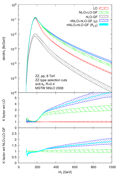
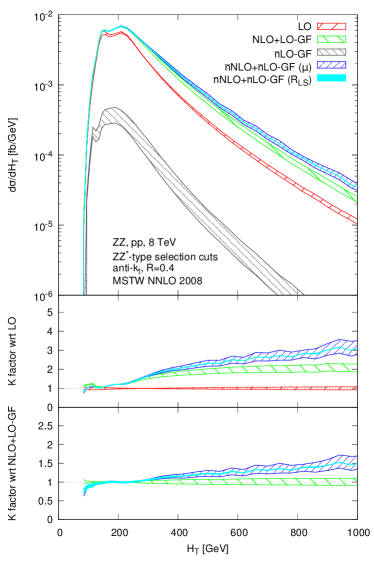
Figure 2: Differential cross sections and K factors for the effective mass observable $H_{T}$, defined in Eq. (7), for the LHC at $\sqrt{s}=8\,\text{TeV}$. The left and the right plot correspond to the $ZZ$ and $ZZ^{*}$ selections defined in Eq. (6). The bands correspond to varying $\mu_{F}=\mu_{R}$ by factors 1/2 and 2 around the central value from Eq. (4). The cyan solid bands give the uncertainty related to the $R_{\text{LS}}$ parameter varied between 0.5 and 1.5. The distribution is a sum of contributions from same-flavor decay channels ($4e$ and $4\mu$) and the different-flavor channel ($2e2\mu$).

Figure 3: Example diagrams contributing to $ZZ$ production at LO, NLO and NNLO.

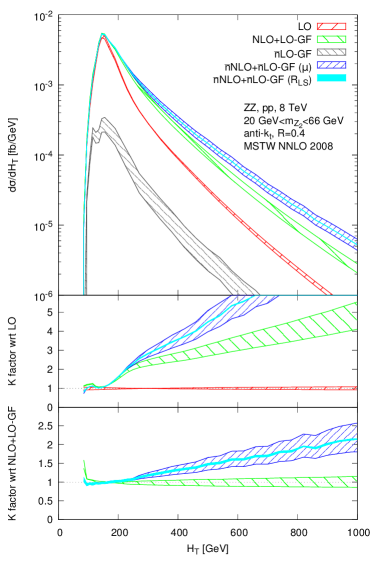
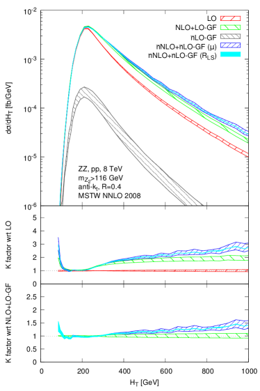
Figure 4: Differential cross sections and K factors for the effective mass observable $H_{T}$, defined in Eq. (7) for the LHC at $\sqrt{s}=8\,\text{TeV}$. The left plot corresponds to the part of $ZZ^{*}$ selection, Eq. (6), where $20<m_{Z}<66\,\mathrm{GeV}$, and the right plot to the part of $ZZ^{*}$ selection with $m_{Z}>116\,\mathrm{GeV}$. Other details are as in Fig. 2.

Fig. 2 shows distributions of the effective mass observable, $H_{T}$, defined as a scalar sum of the transverse momenta of leptons and jets, and missing transverse energy

$$H_{T}=\sum p_{T,\text{jets}}+\sum p_{T,l}+E_{T,\text{miss}}\,.$$ (7)

The left panel corresponds to the $ZZ$ and the right panel to the $ZZ^{*}$ types of cuts. In the former case, the K factor is very large, both at NLO and at $\bar{n}$NLO. In the case of $ZZ^{*}$ selection, the K factor is visibly smaller. The leading correction to this observable at NLO comes from configurations, shown in the middle diagram of Fig. 3, with one of the bosons emitted collinearly and the other with large transverse momentum recoiling against a hard jet $p_{T,{\,\mathrm{jet}}}\simeq p_{T,Z}$ [72], which results in a dependence given by

$$\frac{d\sigma}{d\Omega}\propto\ln\frac{p_{T,{\,\mathrm{jet}}}^{2}}{m_{Z}^{2}}\,.$$ (8)

A similar enhancement occurs at NNLO, where both $Z$ bosons are allowed to be soft or collinear and the result is dominated by the dijet type configurations shown in Fig. 3 (right). This explains both why the K factors grow with transverse momentum and shows that the rate of this growth depends on the selection of the vector boson mass.

In Fig. 4, we split the result of Fig. 2 (right) into the two separate mass regions for the off-shell bosons: $20<m_{Z_{2}}<66\,\mathrm{GeV}$ Fig. 4 (left) and $m_{Z_{2}}>116\,\mathrm{GeV}$ Fig. 4 (right). We see that the NLO and the $\bar{n}$NLO K factors are much larger in the former case, as putting a smaller mass in Eq. (8) leads to a stronger logarithmic enhancement. We also see that, at large $H_{T}$, it is the right plot of Fig. 4 that contributes more to the sum shown in Fig. 2 (right), in terms of absolute values. This comes from the fact that the born cross section is already significantly larger in this case. Therefore, Fig. 4 (right), with larger $m_{Z}$ values, which based on Eq. (8) results in a lower K factor, dominates the total result of Fig. 2 (right). That is why the enhancement is smaller there, as compared to Fig. 2 (left), where only the mass region around the $Z$ peak is included.

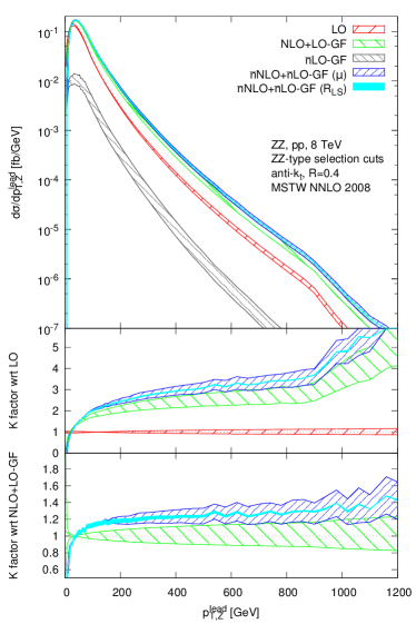
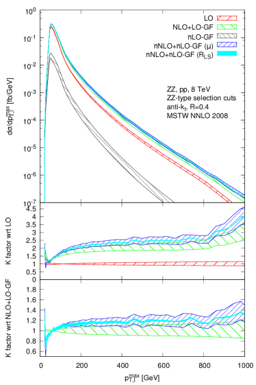
Figure 5: Differential cross sections and K factors for the transverse momentum of the leading $Z$ boson (left) and the leading lepton (right) for the $ZZ$ type selection of Eq. (6) at the LHC with $\sqrt{s}=8\,\text{TeV}$. All details as in Fig. 2.

Let us now turn to Fig. 5, where we show distributions of the transverse momentum of the leading $Z$ boson and that of the leading lepton for the $ZZ$ selection. We see that, in both cases, the $\bar{n}$NLO correction is significant, reaching up to 20% with respect to the NLO result at high $p_{T}$. This magnitude of $\bar{n}$NLO correction at high $p_{T}$ is similar to the one already found in $WZ$ [14] and $WW$ [15] production. We note that, above 200 GeV, the $R_{\,\mathrm{LS}}$ uncertainty is much smaller than the uncertainty coming from variations of the factorization and renormalization scales. Hence, the error related to assigning emission sequence by LoopSim is negligible. The overall theoretical uncertainty decreases by 20-30% as we go from NLO to $\bar{n}$NLO for these distributions. We consider the $\bar{n}$NLO predictions shown in Fig. 5 as one of the highlights of our study. We emphasize that the inclusion of QCD corrections of that size should be mandatory in all related diboson analyses at high transverse momenta. Such large corrections are of huge importance and should be accounted for both in computations of SM backgrounds and in searches for anomalous couplings.

We notice that the kink around 900 $\,\mathrm{GeV}$ in the $p_{T,Z}^{\text{lead}}$ distribution is due to the $\Delta R_{\ell,\ell}$ cut of Eq. (5). For a high-$p_{T}$ boson, the decay products are highly collimated with the $Z$ transverse momentum and they share approximately equal amounts of its $p_{T}$. Hence, the mass of the dilepton system can be approximated by $m^{2}_{\ell\ell}\simeq\frac{1}{4}p_{T,Z}^{2}\Delta R^{2}_{\ell,\ell}$. The imposed phase-space cut $\Delta R_{\ell,\ell}>0.2$ then leads to the condition $p_{T,Z}\lesssim 10\,m_{\ell\ell}$. Since the $m_{\ell,\ell}$ distribution is strongly peaked at the $Z$ boson mass, we obtain that the typical separation between the leptons drops below 0.2 at $p_{T,Z}\simeq 900\,\mathrm{GeV}$. This leads to the kink observed in the LO distribution of Fig. 5. Also, because the two $Z$ bosons are back-to-back in LO configurations and hence have the same $p_{T}$, the same effect happens simultaneously for both $Z$ bosons. With additional parton radiation, this effect is smoothed out. The sub-leading $Z$ boson will in general have a smaller $p_{T}$, as some transverse momentum is carried by the parton. The kink at about 800 GeV in the $p_{T,\ell}^{\text{max}}$ distribution, shown in the right panel of Fig. 5, is also due to the $\Delta R_{\ell,\ell}$ cut. We have checked explicitly that changing the $\Delta R_{\ell,\ell}$ cut to 0.4 moves the kink to 450 and 400 GeV for the $p_{T,Z}^{\text{lead}}$ and $p_{T,\ell}^{\text{max}}$ distribution, respectively, consistent with the above discussion.

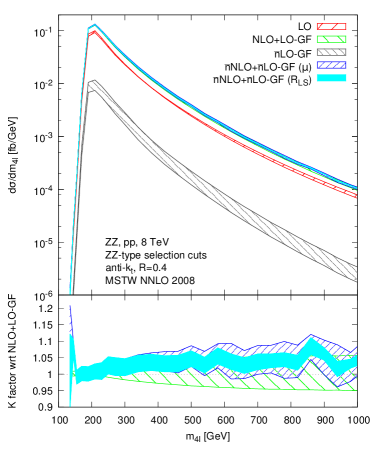
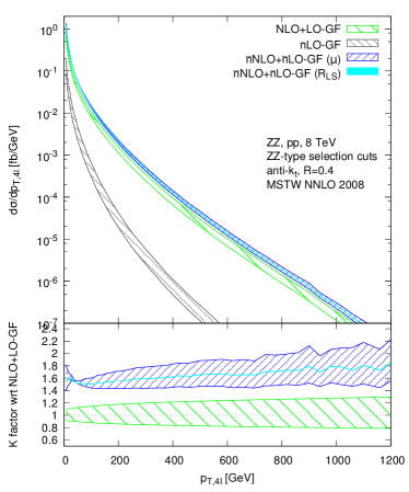
Figure 6: Differential cross sections and K factors for invariant mass (left) and the transverse momentum (right) of the four-lepton system for the $ZZ$ -type selection of Eq. (6) at the LHC with $\sqrt{s}=8\,\text{TeV}$. All details as in Fig. 2.

Another interesting distribution is the mass of the $ZZ$ system or, equivalently, the mass of the system of four leptons, $m_{4\ell}$, which is shown in Fig. 6. This observable is particularly important from the point of view of anomalous triple gauge coupling (aTGC) searches, as the effects of anomalous couplings are enhanced in events where large momentum is transferred through the triple-boson vertex [7, 8]. Such events result in a large invariant mass of the di-boson system. It is interesting to find that the $m_{4\ell}$ distribution receives only modest $\bar{n}$NLO corrections from QCD, which stay always below 5%. This is to be compared with typical sizes of electro-weak corrections, which are not accounted for, and can be of the order of 10% in the tail of the distributions, and with the PDF uncertainties, estimated at 5-10%. Hence, compared to the above sources of uncertainties, the $\bar{n}$NLO QCD corrections are small and we conclude that the $m_{4\ell}$ distribution becomes stable at this order and can be safely used for setting aTGC limits [7, 8].

Fig. 6 (right) shows the distribution of the transverse momentum of the four-lepton system. At LO, this distribution is just a $\delta$-function at $p_{T,4\ell}=0$, since there is no jet the four-lepton system could recoil against. We do not show this first bin in the figure. The first non-trivial order for this observable is then NLO. As we go to $\bar{n}$NLO, the $p_{T,4\ell}$ distribution receives significant corrections of the order of 60-80% for the range presented in the plot, consistent with the NLO predictions shown for $ZZ$+jet production in Ref. [26].

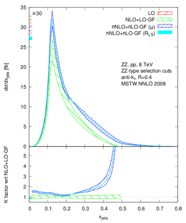
Figure 7: Differential cross sections and K factors at various perturbative orders for the $x_{\,\mathrm{jet}}$ variable defined in Eq. (9). The results correspond to the LHC with $\sqrt{s}=8\,\text{TeV}$ and $ZZ$ -type selection of Eq. (6). All details as in Fig. 2.

Finally, in Fig. 7, we show the distribution of the $x_{\,\mathrm{jet}}$ variable defined as

$$x_{\,\mathrm{jet}}=\frac{\sum_{\begin{subarray}{c}k\in\{{\text{jets}}\end{subarray}\}}E_{T,k}}{\sum_{\begin{subarray}{c}k\in\{{\text{jets},Z\text{s}}\end{subarray}\}}E_{T,k}}\,,$$ (9)

which has been introduced in Ref. [73] in the context of a dynamical jet veto. Large values of this variable correspond to configurations where most of the energy of the final state is carried by jets. For the case of $ZZ$ production, $x_{\,\mathrm{jet}}=0$ at LO and the distribution starts to be non-trivial at NLO. Here we now also show the first bin, which almost exclusively consists of the $x_{\,\mathrm{jet}}=0$ contributions, and which we have scaled down by a factor 30 to fit the plot range. At LO, including LO-GF, the result is simply the inclusive cross section of the process. At higher orders, this bin corresponds effectively to the contribution after placing a jet veto on the process.

As we see in Fig. 7, at NLO, where one jet is allowed, the $x_{\,\mathrm{jet}}$ distribution is peaked around 0.1-0.15, hence, for most events, the jet carries 10-15% fraction of the final state energy. We also see, however, that there is a non-negligible tail reaching out to $x_{\,\mathrm{jet}}=0.5$. When we move to $\bar{n}$NLO, the yield of $x_{\,\mathrm{jet}}$ events increases over the entire range of the distribution at the expense of the energy carried by the $Z$ bosons. In particular, the tail receives corrections with K factors of the order of 5 around $x_{\,\mathrm{jet}}=0.5$. The $\bar{n}$NLO result suggests that the $x_{\,\mathrm{jet}}$ cut, used in dynamical jet veto analyses [73], should be set around $x_{\,\mathrm{jet}}=0.2$, somewhat lower than what could be inferred from the NLO distribution. The $R_{\,\mathrm{LS}}$ uncertainty is negligible for this observable and the renormalization and factorization scale uncertainty is comparable at NLO and $\bar{n}$NLO.

3.2.2 Higgs analysis

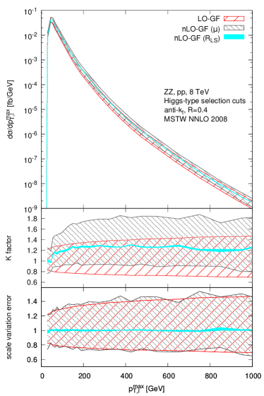
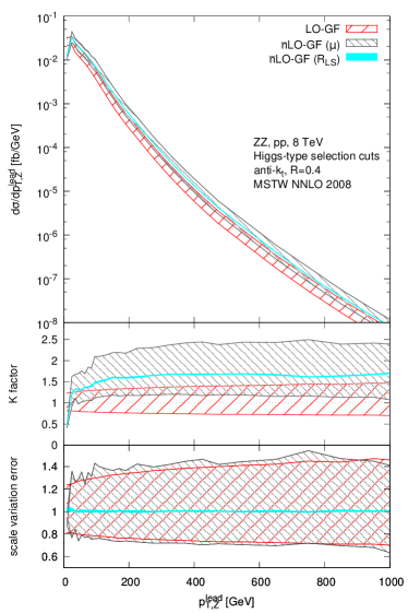
Figure 8: Differential cross sections and K factors for transverse momentum of the leading lepton (left) and the leading $Z$ boson (right) for the Higgs-type selection defined in Eqs. (10) and (11). The results correspond to the LHC at $\sqrt{s}=8\,\text{TeV}$. All other details as in Fig. 2.

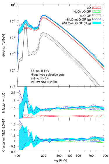
Figure 9: Differential cross sections and K factors for the invariant mass of the four-lepton system for the Higgs-type selection defined in Eqs. (10) and (11). The results correspond to the LHC at $\sqrt{s}=8\,\text{TeV}$. All other details as in Fig. 2.

We turn now to the discussion of the four-lepton production in the context of Higgs analyses. As explained in Section 2 and shown in Fig. 1, the same $ZZ\to 4\ell$ signature can be produced with and without the intermediate Higgs boson. The latter constitutes an irreducible background from the point of view of studies of Higgs production in gluon-gluon fusion, therefore, its precise determination is of utmost importance. The analyses optimized for Higgs studies use slightly different set of cuts with respect to those employed for aTGC searches.

Following the CMS analyses of Ref. [74], where Higgs properties are studied, we require

$$p_{t,e} >7\,\mathrm{GeV}\,, |\eta_{e}|<2.5\,,$$

$$p_{t,\mu} >5\,\mathrm{GeV}\,, |\eta_{\mu}|<2.4\,,$$ (10)

$$p_{t,\ell_{\text{hardest}}} >20\,\mathrm{GeV}\,, m_{4\ell}>100\,\mathrm{GeV}\,,$$

$$p_{t,\ell_{\text{second-hardest}}} >10\,\mathrm{GeV}\,,$$

and

$$40<m_{\ell\ell}<120\,\mathrm{GeV} \text{for the $\ell\ell$ pair with mass closer to $m_{Z}$},$$

$$12<m_{\ell\ell}<120\,\mathrm{GeV} \text{for the other $\ell\ell$ pair},$$ (11)

$$m_{\ell\ell}>4\,\mathrm{GeV} \text{for any oppositely-charged pair of leptons}.$$

We start by showing in Fig. 8 the distributions of transverse momenta of the leading $Z$ and the leading lepton, focusing only on the GF part. The LO result corresponds exactly to the diagrams of Fig. 1 (c) and (d). The $\bar{n}$LO correction is computed with LoopSim using the $gg\to 4\ell+j$ result of Ref. [22] provided by VBFNLO. We see that the correction to $p_{T,Z}^{\text{lead}}$ and $p_{T,\ell}^{\text{lead}}$ is large practically over the entire range shown in Fig. 8. The K factor reaches up to 50% for central values and the scale variation does not decrease as we go from LO to $\bar{n}$LO (bottom panel). It is important to notice that the $R_{\,\mathrm{LS}}$ uncertainty is negligible for those distributions, hence our prediction is very reliable within the uncertainty coming from the factorization and renormalization scale.

Let us now turn to the distribution of the invariant mass of the $ZZ$ pair. As argued in Ref. [1], even though the Higgs width is extremely small in the Standard Model, interference effects between continuum and Higgs-mediated contributions (diagrams (c) and (d) in Fig. 1) lead to enhanced four-lepton mass spectra in the region $m_{4\ell}>2m_{Z}$. Hence, the off-shell effects cannot be neglected, and, as shown recently [2, 3], by comparing the yield at the Higgs mass peak with that off the peak, they can be used for setting bounds on the Higgs decay width.

Our predictions for the four-lepton mass spectra are shown in Fig. 9. Similarly to the $ZZ$ selection discussed in the previous section, also here, $\bar{n}$NLO QCD effects bring a very small correction to this observable. Hence, the $m_{4\ell}$ distribution is stable at this order. This is important from the point of view of the off-shell effect studies in GF fusion, since a precise determination of the expected theoretical yield has impact on setting the Higgs width limits.

4 Summary

We have studied the $ZZ$ production process at the LHC beyond NLO in QCD by merging the $ZZ$ and $ZZ$+jet NLO samples with help of the LoopSim method. We have included the exact, loop-induced GF predictions, which are part of NNLO, as well as the GF $ZZ$+jet contribution, which is formally of N³LO. The NLO samples were obtained with the VBFNLO package. The leptonic decays of the $Z$ bosons, including all off-shell and spin correlation effects, have been fully taken into account.

We have compared the fully inclusive cross section predictions from our framework with the exact results computed in Ref. [32] and found a very good agreement within 2$\%$, covered by the remaining scale uncertainties, despite the fact that the LoopSim method is missing some finite parts originating from the two-loop virtual contributions. Following closely two experimental setups, one used in the SM $ZZ$ production and aTGC searches, and the other used in Higgs analyses, we obtained results for a selection of differential distributions.

For the observables sensitive to QCD radiation, the corrections exceed the errors bars of the NLO predictions combined with the LO-GF results and range from 20$\%$, in the case of the transverse momentum of the $Z$ boson or the leading lepton, up to 100$\%$ for the effective mass variable $H_{T}$. A study of the $x_{\text{jet}}$ observable, defined as ratio of the transverse energy sum of the jets over the sum of transverse energies of jets and $Z$ bosons, shows that the $\bar{n}$NLO corrections start to increase quickly when this variable exceeds $0.2$. Therefore, when this variable is used to impose a dynamical jet veto, a cut should be placed at around this value. For Higgs-type selection, we investigated also the $ZZ$ production via GF at $\bar{n}$LO. The size of the corrections are around 50$\%$ for the transverse momenta of the leading $Z$ and 20$\%$ for those of the leading lepton.

For observables which favor the LO kinematics, like $m_{4l}$, the approximated NNLO QCD corrections are small, of the order of 5$\%$, and comparable with the size of the remaining scale or PDF uncertainties.

Modifications to the VBFNLO program used in this article are available on request and will be part of a future release. The LoopSim library, together with the Les Houches Event interface, is publicly available at https://loopsim.hepforge.org.

References

- [1] N. Kauer and G. Passarino, JHEP 1208 (2012) 116 [arXiv:1206.4803 [hep-ph]].
- [2] F. Caola and K. Melnikov, Phys. Rev. D 88 (2013) 054024 [arXiv:1307.4935 [hep-ph]].
- [3] J. M. Campbell, R. K. Ellis and C. Williams, JHEP 1404 (2014) 060
- [4] J. S. Gainer, J. Lykken, K. T. Matchev, S. Mrenna and M. Park, Phys. Rev. D 91, no. 3, 035011 (2015) [arXiv:1403.4951 [hep-ph]].
- [5] C. Englert and M. Spannowsky, Phys. Rev. D 90 (2014) 5, 053003 [arXiv:1405.0285 [hep-ph]].
- [6] G. Cacciapaglia, A. Deandrea, G. Drieu La Rochelle and J. B. Flament, Phys. Rev. Lett. 113, no. 20, 201802 (2014) [arXiv:1406.1757 [hep-ph]].
- [7] G. Aad et al. [ATLAS Collaboration], JHEP 1303 (2013) 128
- [8] V. Khachatryan et al. [CMS Collaboration], arXiv:1406.0113 [hep-ex].
- [9] B. Mele, P. Nason and G. Ridolfi, Nucl. Phys. B 357 (1991) 409.
- [10] J. Ohnemus and J. F. Owens, Phys. Rev. D 43 (1991) 3626.
- [11] J. M. Campbell and R. K. Ellis, Phys. Rev. D 60 (1999) 113006 [hep-ph/9905386].
- [12] L. J. Dixon, Z. Kunszt and A. Signer, Phys. Rev. D 60 (1999) 114037 [hep-ph/9907305].
- [13] M. Rubin, G. P. Salam and S. Sapeta, JHEP 1009 (2010) 084.
- [14] F. Campanario and S. Sapeta, Phys. Lett. B 718 (2012) 100
- [15] F. Campanario, M. Rauch and S. Sapeta, Nucl. Phys. B 879 (2014) 65
- [16] D. A. Dicus, C. Kao and W. W. Repko, Phys. Rev. D 36 (1987) 1570.
- [17] E. W. N. Glover and J. J. van der Bij, Phys. Lett. B 219 (1989) 488.
- [18] T. Matsuura and J. J. van der Bij, Z. Phys. C 51 (1991) 259.
- [19] C. Zecher, T. Matsuura and J. J. van der Bij, Z. Phys. C 64 (1994) 219 [hep-ph/9404295].
- [20] N. E. Adam, T. Aziz, J. R. Andersen, A. Belyaev, T. Binoth, S. Catani, M. Ciccolini and J. E. Cole et al., arXiv:0803.1154 [hep-ph].
- [21] T. Binoth, N. Kauer and P. Mertsch, arXiv:0807.0024 [hep-ph].
- [22] F. Campanario, Q. Li, M. Rauch and M. Spira, JHEP 1306 (2013) 069 [arXiv:1211.5429 [hep-ph]].
- [23] F. Caola, J. M. Henn, K. Melnikov, A. V. Smirnov and V. A. Smirnov, arXiv:1503.08759 [hep-ph].
- [24] A. Bierweiler, T. Kasprzik and J. H. Kühn, JHEP 1312 (2013) 071 [arXiv:1305.5402 [hep-ph]].
- [25] J. Baglio, L. D. Ninh and M. M. Weber, arXiv:1310.3972 [hep-ph].
- [26] T. Binoth, T. Gleisberg, S. Karg, N. Kauer and G. Sanguinetti, Phys. Lett. B 683 (2010) 154 [arXiv:0911.3181 [hep-ph]].
- [27] F. Campanario, M. Kerner, L. D. Ninh and D. Zeppenfeld, JHEP 1407 (2014) 148 [arXiv:1405.3972 [hep-ph]].
- [28] T. Gehrmann, A. von Manteuffel, L. Tancredi and E. Weihs, JHEP 1406 (2014) 032 [arXiv:1404.4853 [hep-ph]].
- [29] F. Caola, J. M. Henn, K. Melnikov, A. V. Smirnov and V. A. Smirnov, JHEP 1411 (2014) 041 [arXiv:1408.6409 [hep-ph]].
- [30] T. Gehrmann, A. von Manteuffel and L. Tancredi, arXiv:1503.04812 [hep-ph].
- [31] A. von Manteuffel and L. Tancredi, arXiv:1503.08835 [hep-ph].
- [32] F. Cascioli, T. Gehrmann, M. Grazzini, S. Kallweit, P. Maierhöfer, A. von Manteuffel, S. Pozzorini and D. Rathlev et al., Phys. Lett. B 735 (2014) 311 [arXiv:1405.2219 [hep-ph]].
- [33] M. Rubin, G. P. Salam and S. Sapeta, https://loopsim.hepforge.org.
- [34] K. Arnold, M. Bahr, G. Bozzi, F. Campanario, C. Englert, T. Figy, N. Greiner and C. Hackstein et al., Comput. Phys. Commun. 180 (2009) 1661 [arXiv:0811.4559 [hep-ph]].
- [35] K. Arnold, J. Bellm, G. Bozzi, M. Brieg, F. Campanario, C. Englert, B. Feigl and J. Frank et al., arXiv:1107.4038 [hep-ph].
- [36] J. Baglio, J. Bellm, F. Campanario, B. Feigl, J. Frank, T. Figy, M. Kerner and L. D. Ninh et al., arXiv:1404.3940 [hep-ph].
- [37] D. Maitre and S. Sapeta, Eur. Phys. J. C 73 (2013) 12, 2663
- [38] S. Chatrchyan et al. [CMS Collaboration], Phys. Lett. B 716 (2012) 30
- [39] L. D. Landau, Dokl. Akad. Nauk Ser. Fiz. 60, 207 (1948).
- [40] C. N. Yang, Phys. Rev. 77, 242 (1950).
- [41] F. Campanario, C. Englert, M. Rauch and D. Zeppenfeld, Phys. Lett. B 704 (2011) 515 [arXiv:1106.4009 [hep-ph]].
- [42] K. Hagiwara and D. Zeppenfeld, Nucl. Phys. B 313 (1989) 560.
- [43] F. Campanario, JHEP 1110 (2011) 070 [arXiv:1105.0920 [hep-ph]].
- [44] G. ’t Hooft and M. J. G. Veltman, Nucl. Phys. B 44 (1972) 189.
- [45] M. S. Chanowitz, M. Furman and I. Hinchliffe, Nucl. Phys. B 159 (1979) 225.
- [46] S. Catani and M. H. Seymour, Nucl. Phys. B 485 (1997) 291 [Erratum-ibid. B 510 (1998) 503] [hep-ph/9605323].
- [47] G. ’t Hooft and M. J. G. Veltman, Nucl. Phys. B 153 (1979) 365.
- [48] Z. Bern, L. J. Dixon and D. A. Kosower, Nucl. Phys. B 412 (1994) 751 [hep-ph/9306240].
- [49] S. Dittmaier, Nucl. Phys. B 675 (2003) 447 [hep-ph/0308246].
- [50] G. Passarino and M. J. G. Veltman, Nucl. Phys. B 160 (1979) 151.
- [51] T. Hahn and M. Rauch, Nucl. Phys. Proc. Suppl. 157 (2006) 236 [hep-ph/0601248].
- [52] T. Binoth, J. P. Guillet, G. Heinrich, E. Pilon and C. Schubert, JHEP 0510 (2005) 015 [hep-ph/0504267].
- [53] A. Denner and S. Dittmaier, Nucl. Phys. B 734 (2006) 62 [hep-ph/0509141].
- [54] T. Hahn, Nucl. Phys. Proc. Suppl. 89 (2000) 231 [hep-ph/0005029].
- [55] T. Hahn, Comput. Phys. Commun. 178 (2008) 217 [hep-ph/0611273].
- [56] M. Rauch, arXiv:0804.2428 [hep-ph].
- [57] C. Groß, T. Hahn, S. Heinemeyer, F. von der Pahlen, H. Rzehak and C. Schappacher, PoS LL 2014 (2014) 035.
- [58] T. Gleisberg, S. Hoeche, F. Krauss, M. Schonherr, S. Schumann, F. Siegert and J. Winter, JHEP 0902 (2009) 007 [arXiv:0811.4622 [hep-ph]].
- [59] J. M. Campbell and R. K. Ellis, Nucl. Phys. Proc. Suppl. 205-206 (2010) 10 [arXiv:1007.3492 [hep-ph]].
- [60] A. Denner, S. Dittmaier, M. Roth and D. Wackeroth, Nucl. Phys. B 560 (1999) 33 [hep-ph/9904472].
- [61] J. Alwall, A. Ballestrero, P. Bartalini, S. Belov, E. Boos, A. Buckley, J. M. Butterworth and L. Dudko et al., Comput. Phys. Commun. 176 (2007) 300 [hep-ph/0609017].
- [62] Y. L. Dokshitzer, G. D. Leder, S. Moretti and B. R. Webber, JHEP 9708 (1997) 001 [arXiv:hep-ph/9707323].
- [63] M. Wobisch and T. Wengler, arXiv:hep-ph/9907280.
- [64] M. Cacciari and G. P. Salam, Phys. Lett. B 641 (2006) 57
- [65] M. Cacciari, G. P. Salam and G. Soyez, http://fastjet.fr/ .
- [66] S. Catani, Y. L. Dokshitzer, M. Olsson, G. Turnock and B. R. Webber, Phys. Lett. B 269, 432 (1991);
- [67] S. D. Ellis and D. E. Soper, Phys. Rev. D 48 (1993) 3160 [hep-ph/9305266].
- [68] A. D. Martin, W. J. Stirling, R. S. Thorne and G. Watt, Eur. Phys. J. C 63 (2009) 189 [arXiv:0901.0002 [hep-ph]].
- [69] M. Cacciari, G. P. Salam and G. Soyez, JHEP 0804 (2008) 063
- [70] M. Cacciari, G. P. Salam and G. Soyez, Eur. Phys. J. C 72 (2012) 1896
- [71] M. R. Whalley, D. Bourilkov and R. C. Group, hep-ph/0508110.
- [72] S. Frixione, P. Nason and G. Ridolfi, Nucl. Phys. B 383 (1992) 3.
- [73] F. Campanario, R. Roth and D. Zeppenfeld, Phys. Rev. D 91 (2015) 5, 054039 [arXiv:1410.4840 [hep-ph]].
- [74] [CMS Collaboration], CMS-PAS-HIG-13-002.