Modified Laplacian coflow of $G_{2}$-structures on manifolds with symmetry

Abstract

We consider $G_{2}$-structures on $7$-manifolds that are warped products of an interval and a six-manifold, which is either a Calabi-Yau manifold, or a nearly Kähler manifold. We show that in these cases the $G_{2}$-structures are determined by their torsion components up to a phase factor. We then study the modified Laplacian coflow $\frac{d\psi}{dt}=\Delta_{\psi}\psi+2d\left(\left(C-\mathop{\mathrm{T}r}T\right)\varphi\right)$ of these $G_{2}$-structures, where $\varphi$ and $\psi$ are the fundamental $3$-form and $4$-form which define the $G_{2}$-structure and $\Delta_{\psi}$ is the Hodge Laplacian associated with the $G_{2}$-structure. This flow is known to have short-time existence and uniqueness. We analyse the soliton equations for this flow and obtain new compact soliton solutions.

1 Introduction

Geometric flows play a very important role in the study of various geometric objects. Flows of $G_{2}$-structures on $7$-dimensional manifolds have been first introduced by Robert Bryant in [3]. The original Laplacian flow of $G_{2}$-structures was given by

$$\frac{\partial\varphi}{\partial t}=\Delta_{\varphi}\varphi$$ (1.1)

where $\varphi$ is the $3$-form that defines the $G_{2}$-structure (and hence the metric), and $\Delta_{\varphi}=dd^{\ast}+d^{\ast}d$ is the Hodge Laplacian associated with this $G_{2}$-structure. In general, this is a non-parabolic, non-linear PDE for $\varphi$ [13]. However, if initially $\varphi$ is a closed (or sometimes known as calibrated) $G_{2}$-structure, that is when $d\varphi=0$, the flow (1.1) becomes a flow of closed $G_{2}$-structures (since $\Delta_{\varphi}\varphi=dd^{\ast}\varphi$ becomes an exact form), and acquires much nicer properties. This flow of closed $G_{2}$-structures can then be interpreted as the gradient flow of Hitchin’s volume functional [14]. Also, as it has been shown in [4, 23], it has short-time existence and uniqueness, and moreover a stability property [23]. There has also been work done on related flows of $G_{2}$-structures - such as heat flows by Weiss-Witt [22, 21] and a general overview of flows of $G_{2}$-structures by Karigiannis [18], as well as the Laplacian coflow of co-closed $G_{2}$-structures, which was introduced by Karigiannis-McKay-Tsui in [19]. This was a Laplacian flow $\frac{\partial\psi}{\partial t}=-\Delta_{\psi}\psi$ of the dual $4$-form $\psi=\ast_{\varphi}\varphi$ which is now assumed to be closed, so that $\Delta_{\psi}\psi$ is an exact form and preserves the closed property of $\psi.$ It was later shown by the current author in [13] that the Laplacian flow of co-closed $G_{2}$-structures is not even a weakly parabolic flow, and in fact the symbol of the operator $\Delta_{\psi}\psi$ has a mixed signature. Therefore, a modified Laplacian coflow was introduced in [13]:

$$\frac{d\psi}{dt}=\Delta_{\psi}\psi+2d\left(\left(C-\mathop{\mathrm{T}r}T\right)\varphi\right).$$ (1.2)

Here $\mathop{\mathrm{T}r}T$ is the trace of the torsion tensor of the $G_{2}$-structure defined by the $4$-form $\psi$ and $C$ is any constant. Note that if $\psi$ is co-closed, then the right hand side of (1.2) is exact and hence the flow preserves the cohomology class of $\psi$ in the same way as the original Laplacian coflow. The flow (1.2) is weakly parabolic in the direction of closed forms and short-time existence and uniqueness of solutions was shown in [13].

In [19] the authors have considered the behavior of the original coflow on manifolds with symmetry - in particular, where the $7$-manifold is a warped product of 1-dimensional space $L$ (either a line interval or a circle) and a six-dimensional space $N^{6}$ - which is either a Calabi-Yau or a nearly Kähler manifold. As originally shown by Ivanov and Cleyton in [7], $G_{2}$-structures on such warped product manifolds always have a vanishing $14$-dimensional torsion component, which excludes the possibility of them admitting a non-torsion-free closed $G_{2}$-structure. However, the $7$-dimensional torsion component can be set to zero, leaving only the symmetric part of the torsion tensor, and this gives a co-closed $G_{2}$-structure. Therefore, it is natural to study flows of co-closed $G_{2}$-structures on these manifolds. In this case, the complicated PDEs from the general case then become more manageable since the spatial part of the equation reduces to a 1-dimensional problem on $L$. Furthermore, if soliton solutions are considered, the equations reduce to a system of ODEs which can be solved explicitly in some cases. In this paper we will produce a similar analysis, but for the modified flow (1.2).

The outline of the paper is following. In Section 2 we give an introduction to $G_{2}$-structures and torsion and in Section 3 we specialize to the case of the warped product manifold $N^{6}\times L$. We rederive the expression for the torsion components of a $G_{2}$-structure on such a product manifold and give an expression for the full torsion tensor. In particular, we also show that generically, in this case, the torsion components in fact determine the $G_{2}$-structure up to a phase factor. We express the torsion in terms of parameters $\alpha,\beta,\gamma$ and show how they give the $G_{2}$-structure. The parameters $\alpha$ and $\beta$ determine the $\mathbf{1\oplus 27}$ part of the torsion, while $\gamma$ determines the $\mathbf{7}$ part of the torsion. The restriction to co-closed $G_{2}$-structures is then equivalent to setting $\gamma=0$. In Section 4, we then express the Laplacian of the $G_{2}$-structure in terms of $\alpha,\beta,\gamma$ and in Section 5 we derive the modified Laplacian coflow (1.2) for the warped product $G_{2}$-structure. In the special case where $N^{6}$ is a Calabi-Yau manifold, and when $C=0$ in (1.2) we find explicit separable solutions, which, as expected, blow up in finite time. Finally, in Section 6, we specialize to soliton solutions of (1.2). The equations that we obtain are a system of three nonlinear first order ODEs, which are similar to the third order nonlinear ODE obtained in [19] for the standard Laplacian coflow. However, due to the extra freedom that we get by including the constant $C$ in (1.2), we are able to obtain new non-trivial solutions. In particular, in the case when $N^{6}$ is a Calabi-Yau manifold, we obtain explicit solutions that are periodic and are thus defined when $L\cong S^{1}.$ Hence these are compact soliton solutions. In the more complicated case when $N^{6}$ is nearly Kähler, the equations are still very difficult to analyze, however we systematically consider solutions where at least one of the dependent variables is constant. This way we recover some of the solutions given in [19], as well as new solutions.

2 $G_{2}$-structures and torsion

The 14-dimensional group $G_{2}$ is the smallest of the five exceptional Lie groups and is closely related to the octonions. In particular, $G_{2}$ can be defined as the automorphism group of the octonion algebra. Taking the imaginary part of octonion multiplication of the imaginary octonions defines a vector cross product on $V=\mathbb{R}^{7}$ and the group that preserves the vector cross product is precisely $G_{2}$. A more detailed account of the relationship between octonions and $G_{2}$ can be found in [1, 11].The structure constants of the vector cross product define a $3$-form on $\mathbb{R}^{7}$, hence $G_{2}$ can alternatively be defined as the subgroup of $GL\left(7,\mathbb{R}\right)$ that preserves a particular $3$-form [16]. In general, given an $n$-dimensional manifold $M$, a $G$-structure on $M$ for some Lie subgroup $G$ of $GL\left(n,\mathbb{R}\right)$ is a reduction of the frame bundle $F$ over $M$ to a principal subbundle $P$ with fibre $G$. A $G_{2}$-structure is then a reduction of the frame bundle on a $7$-dimensional manifold $M$ to a $G_{2}$ principal subbundle. It turns out that there is a $1$-$1$ correspondence between $G_{2}$-structures on a $7$-manifold and smooth $3$-forms $\varphi$ for which the $7$-form-valued bilinear form $B_{\varphi}$ as defined by (2.1) is positive definite (for more details, see [2] and the arXiv version of [15]).

$$B_{\varphi}\left(u,v\right)=\frac{1}{6}\left(u\lrcorner\varphi\right)\wedge\left(v\lrcorner\varphi\right)\wedge\varphi$$ (2.1)

Here the symbol $\lrcorner$ denotes contraction of a vector with the differential form:

$$\left(u\lrcorner\varphi\right)_{mn}=u^{a}\varphi_{amn}.$$

Note that we will also use this symbol for contractions of differential forms using the metric.

A smooth $3$-form $\varphi$ is said to be positive if $B_{\varphi}$ is the tensor product of a positive-definite bilinear form and a nowhere-vanishing $7$-form. In this case, it defines a unique metric $g_{\varphi}$ and volume form $\mathrm{vol}$ such that for vectors $u$ and $v$, the following holds

$$g_{\varphi}\left(u,v\right)\mathrm{vol}=\frac{1}{6}\left(u\lrcorner\varphi\right)\wedge\left(v\lrcorner\varphi\right)\wedge\varphi$$ (2.2)

In components we can rewrite this as

$$\left(g_{\varphi}\right)_{ab}=\left(\det s\right)^{-\frac{1}{9}}s_{ab}\ \text{where \ }s_{ab}=\frac{1}{144}\varphi_{amn}\varphi_{bpq}\varphi_{rst}\hat{\varepsilon}^{mnpqrst}.$$ (2.3)

Here $\hat{\varepsilon}^{mnpqrst}$ is the alternating symbol with $\hat{\varepsilon}^{12...7}=+1$. Following Joyce ([16]), we will adopt the following definition

Definition 2.1

The pair $\left(\varphi,g\right)$ for a positive $3$-form $\varphi$ and corresponding metric $g$ defined by (2.2) will be referred to as a $G_{2}$-structure.

Definition 2.2

Given a $G_{2}$-structure $\left(\varphi,g\right)$, define the Hodge star $\ast_{\varphi}$ that is associated with $\left(\varphi,g\right)$, the dual $4$-form $\psi=\ast_{\varphi}\varphi$ and the Laplacian $\Delta_{\varphi}$

Note that up to an overall sign of the orientation, a $G_{2}$-structure can alternatively be defined using the $4$-form $\psi.$ In this case, we will say that $\left(\psi,g\right)$ is a $G_{2}$-structure giving the Hodge star $\ast_{\psi}$ and the Laplacian $\Delta_{\psi}$.

Given a $G_{2}$-structure, the spaces of differential forms decompose orthogonally according to irreducible representation of $G_{2}.$ In particular, $2$-forms split as $\Lambda^{2}=\Lambda_{7}^{2}\oplus\Lambda_{14}^{2}$, where

$$\Lambda_{7}^{2} = \left\{\alpha\lrcorner\varphi\text{: for a vector field }\alpha\right\}$$

$$\Lambda_{14}^{2} = \left\{\omega\in\Lambda^{2}\text{: }\left(\omega_{ab}\right)\in\mathfrak{g}_{2}\right\}=\left\{\omega\in\Lambda^{2}\text{: }\omega\lrcorner\varphi=0\right\}$$

Using Hodge duality, a similar decomposition exists for $5$-forms.

The $3$-forms decompose as $\Lambda^{3}=\Lambda_{1}^{3}\oplus\Lambda_{7}^{3}\oplus\Lambda_{27}^{3}$, where the one-dimensional component consists of forms proportional to $\varphi$, forms in the $7$-dimensional component are defined by a vector field $\Lambda_{7}^{3}=\left\{\alpha\lrcorner\psi\text{: for a vector field }\alpha\right\}$, and forms in the $27$-dimensional component are defined by traceless, symmetric matrices:

$$\Lambda_{27}^{3}=\left\{\chi\in\Lambda^{3}:\chi_{abc}=\mathrm{i}_{\varphi}\left(h\right)=h_{[a}^{d}\varphi_{bc]d}\text{ for }h_{ab}~{}\text{traceless, symmetric}\right\}.$$ (2.4)

Again, by Hodge duality a similar decomposition exists for $4$-forms. A detailed description of these representations is given in [2, 3].

The intrinsic torsion of a $G_{2}$-structure is defined by $\nabla\varphi$, where $\nabla$ is the Levi-Civita connection for the metric $g$ that is defined by $\varphi$. Following [18], it is easy to see

$$\nabla\varphi\in\Lambda_{7}^{1}\otimes\Lambda_{7}^{3}\cong W.$$ (2.5)

Here we define $W$ as the space $\Lambda_{7}^{1}\otimes\Lambda_{7}^{3}$. Given (2.5), we can write

$$\nabla_{a}\varphi_{bcd}=T_{a}^{\ e}\psi_{ebcd}$$ (2.6)

where $T_{ab}$ is the full torsion tensor. We can also invert (2.6) to get an explicit expression for $T$

$$T_{a}^{\ m}=\frac{1}{24}\left(\nabla_{a}\varphi_{bcd}\right)\psi^{mbcd}.$$ (2.7)

This $2$-tensor fully defines $\nabla\varphi$ since pointwise, it has 49 components, and the space $W$ is also 49-dimensional (pointwise). In general we can split $T_{ab}$ according to representations of $G_{2}$ into torsion components:

$$T=\tau_{1}g+\tau_{7}\lrcorner\varphi+\tau_{14}+\tau_{27}$$ (2.8)

where $\tau_{1}$ is a function, and gives the $\mathbf{1}$ component of $T$. We also have $\tau_{7}$, which is a $1$-form and hence gives the $\mathbf{7}$ component, and, $\tau_{14}\in\Lambda_{14}^{2}$ gives the $\mathbf{14}$ component and $\tau_{27}$ is traceless symmetric, giving the $\mathbf{27}$ component. Hence we can split $W$ as

$$W=W_{1}\oplus W_{7}\oplus W_{14}\oplus W_{27}.$$ (2.9)

As it was originally shown by Fernández and Gray [8], there are in fact a total of 16 torsion classes of $G_{2}$-structures that arise as the $G_{2}$-invariant subspaces of $W$ to which $\nabla\varphi$ belongs. Moreover, as shown in [18], the torsion components relate directly to the expression for $d\varphi$ and $d\psi$. In fact, in our notation,

$$d\varphi = 4\tau_{1}\psi-3\tau_{7}\wedge\varphi-3\ast\mathrm{i}_{\varphi}\left(\tau_{27}\right)$$ (2.10a)

$$d\psi = -4\tau_{7}\wedge\psi-2\ast\tau_{14}.$$ (2.10b)

Note that in the literature ([3, 6], for example) a slightly different convention for torsion components is sometimes used. Our $\tau_{1}$ component corresponds to $\frac{1}{4}\tau_{0}$, $\tau_{7}$ corresponds to $-\tau_{1}$ in their notation, $\tau_{14}$ corresponds to $\frac{1}{2}\tau_{2}$ and $\mathrm{i}_{\varphi}\left(\tau_{27}\right)$ corresponds to $-\frac{1}{3}\tau_{3}$ . Similarly, our torsion classes $W_{1}\oplus W_{7}\oplus W_{14}\oplus W_{27}$ correspond to $W_{0}\oplus W_{1}\oplus W_{2}\oplus W_{3}$. In our notation the subscripts denote the dimensionally of the representation, while in the alternative notation the subscripts denote the degree of the corresponding differential form. Also the constant factors are different because we consider the $\tau_{i}$ as components of the full torsion tensor $T$, while in the alternative point of view they are regarded as components of the differential forms $d\varphi$ and $d\psi$.

Definition 2.3

A $G_{2}$-structure is said to be torsion-free if $T=0.$ Equivalently, $d\varphi=0$ and $d\psi=0$ [8].

Definition 2.4

A $G_{2}$-structure is said to be closed if $d\varphi=0.$ Equivalently, $T=\tau_{14}$.

Definition 2.5

A $G_{2}$-structure is said to be co-closed if $d\psi=0$. Equivalently $T=\tau_{1}g+\tau_{27}$, that is, the skew-symmetric part of $T$ vanishes, and the tensor $T$ is thus fully symmetric.

Note that sometimes closed and co-closed $G_{2}$-structures are called calibrated and cocalibrated, respectively.

Example 2.6

A special case of a co-closed $G_{2}$-structure occurs when $\tau_{27}=0$. In this case, we have $d\varphi=4\tau_{1}\psi$ with $\tau_{1}$ constant. $G_{2}$-structures of this type are called nearly parallel, and they are Einstein manifolds, with $Ric=6\tau_{1}^{2}g$. In particular, the round sphere $S^{7}$ admits a nearly parallel $G_{2}$-structure [9].

3 $G_{2}$-structures on warped product manifolds

Consider an $SU\left(3\right)$-structure $\left(g_{6},\omega,\Omega\right)$ on a $6$-manifold $N^{6}$ - where $g_{6}$ is a Riemannian metric, $\omega$ is a compatible Hermitian form of type $\left(1,1\right)$, and $\Omega$ is a nowhere vanishing smooth complex-valued $3$-form of type $\left(3,0\right).$ The $SU\left(3\right)$-structure forms $\omega$ and $\Omega$ satisfy algebraic constraints

$$\Omega\wedge\omega = \bar{\Omega}\wedge\omega=0$$ (3.1a)

$$\omega^{3} = 6\mathop{\mathrm{v}ol}_{6}$$ (3.1b)

$$\Omega\wedge\bar{\Omega} = -8i\mathop{\mathrm{v}ol}_{6}$$ (3.1c)

Since we are restricting our attention to Calabi-Yau and nearly Kähler $6$-manifolds, the exterior derivatives of $\omega$ and $\Omega$ satisfy the following relations

$$d\omega = -3\lambda\mathop{\mathrm{R}e}\Omega$$ (3.2a)

$$= -\frac{3}{2}\lambda\Omega-\frac{3}{2}\lambda\bar{\Omega}$$ (3.2b)

$$d\Omega = 2\lambda i\omega^{2}$$ (3.2c)

$$d\left(\omega^{2}\right) = 0$$ (3.2d)

where $\lambda$ is a constant. Note that $\lambda=0$ corresponds to a Calabi-Yau manifold, and generally we will set $\lambda=1$ for a nearly Kähler manifold. The Ricci curvature $Ric_{6}$ of a nearly Kähler manifold of type $\lambda$ is given by

$$Ric_{6}=5\lambda g_{6}$$ (3.3)

More details on nearly Kähler manifolds are given in [10, 20].

Now suppose $L$ is a $1$-dimensional manifold and consider $M^{7}=N^{6}\times L$ with $r$ a local coordinate on $L$. An induced $G_{2}$-structure on $M^{7}$ is given by

$$\varphi = \mathop{\mathrm{R}e}\Omega+dr\wedge\omega$$ (3.4a)

$$\psi = \frac{1}{2}\omega^{2}+\mathop{\mathrm{I}m}\Omega\wedge dr$$ (3.4b)

$$g_{7} = dr^{2}+g_{6}$$ (3.4c)

More generally, let $F\left(r\right)$ be a smooth, nowhere-vanishing complex-valued function on $L$ and let $G\left(r\right)$ be a smooth, real, everywhere positive function on $L$. Then, following [5, 19] we get a warped product $G_{2}$-structure on $M^{7}$ given by

$$\varphi = \mathop{\mathrm{R}e}\left(F^{3}\Omega\right)+G\left|F\right|^{2}dr\wedge\omega$$ (3.5a)

$$\psi = \frac{1}{2}\left|F\right|^{4}\omega^{2}+\mathop{\mathrm{I}m}\left(F^{3}\Omega\right)\wedge Gdr$$ (3.5b)

$$g_{7} = G^{2}dr^{2}+\left|F\right|^{2}g_{6}$$ (3.5c)

$$\mathop{\mathrm{v}ol}_{7} = G\left|F\right|^{6}\mathop{\mathrm{v}ol}_{6}\wedge dr$$ (3.5d)

We can write

$$F=he^{i\frac{\theta}{3}}$$ (3.6)

Then, the $\varphi,\psi,$ $g_{7}$ and $\mathop{\mathrm{v}ol}_{7}$ from (3.5) can be rewritten as

$$\varphi = \frac{1}{2}F^{3}\Omega+\frac{1}{2}\bar{F}^{3}\bar{\Omega}+Gh^{2}dr\wedge\omega$$ (3.7a)

$$\psi = \frac{1}{2}h^{4}\omega^{2}-\frac{iGF^{3}}{2}\Omega\wedge dr+\frac{iG\bar{F}^{3}}{2}\bar{\Omega}\wedge dr$$ (3.7b)

$$g_{7} = G^{2}dr^{2}+h^{2}g_{6}$$ (3.7c)

$$\mathop{\mathrm{v}ol}_{7} = Gh^{6}\mathop{\mathrm{v}ol}_{6}\wedge dr$$ (3.7d)

Using the expressions for the metric $g_{7}$ and the volume form $\mathop{\mathrm{v}ol}_{7}$, we obtain that if $\alpha$ is a $k$-form on $N^{6},$ then

$$\ast_{7}\alpha = \left(-1\right)^{k}h^{6-2k}Gdr\wedge\ast_{6}\alpha$$ (3.8a)

$$\ast_{7}\left(dr\wedge\alpha\right) = h^{6-2k}G^{-1}\ast_{6}\alpha$$ (3.8b)

From these expression we obtain the following useful formulae.

Corollary 3.1 ([19])

Given the metric $g_{7}$ and the volume form $\mathop{\mathrm{v}ol}_{7}$ as in (3.7c) and (3.7d), the Hodge duals of the $SU\left(3\right)$-equivariant differential forms on $M^{7}$ are:

$$\ast_{7}\omega = \frac{1}{2}h^{2}Gdr\wedge\omega^{2}$$ (3.9a)

$$\ast_{7}\Omega = iGdr\wedge\Omega$$ (3.9b)

$$\ast_{7}\left(\omega^{2}\right) = 2h^{-2}Gdr\wedge\omega$$ (3.9c)

$$\ast_{7}\left(Gdr\wedge\omega\right) = \frac{1}{2}h^{2}\omega^{2}$$ (3.9d)

$$\ast_{7}\left(Gdr\wedge\Omega\right) = -i\Omega$$ (3.9e)

$$\ast_{7}\left(Gdr\wedge\omega^{2}\right) = 2h^{-2}\omega$$ (3.9f)

As noted in [19], we can always redefine the $r$ coordinate in order to set $G=1\,.$ However when looking at a flow of $G_{2}$-structures, the function $G\left(r\right)$ will be time-dependent and hence the reparametrization of $r$. Therefore, in a time-dependent picture it is convenient to keep $G\left(r\right)$ unrestricted.

Any $3$-form $\chi$ on $M^{7}$ that respects the symmetry of the manifold must be a linear combination of $\Omega$, $\bar{\Omega}$ and $dr\wedge\omega$. Therefore, in general, we can write such a $3$-form as

$$\chi=\frac{1}{2}AF^{3}\Omega+\frac{1}{2}\bar{A}\bar{F}^{3}\bar{\Omega}+Gh^{2}Bdr\wedge\omega$$ (3.10)

where $A$ is a smooth complex-valued function on $L$ and $B$ is a smooth real-valued function on $L.$ Hence, such $3$-forms are uniquely defined by three real-valued functions on $L$: $\mathop{\mathrm{R}e}A,$ $\mathop{\mathrm{I}m}A$ and $B$. For a $3$-form given by (3.10), let us use the following notation

$$\mathop{\mathrm{R}e}_{1}\chi = \mathop{\mathrm{R}e}A$$ (3.11a)

$$\mathop{\mathrm{I}m}_{1}\chi = \mathop{\mathrm{I}m}A$$ (3.11b)

$$\mathop{\mathrm{R}e}_{2}\chi = B$$ (3.11c)

Such a decomposition of $\chi$ effectively gives a decomposition according to representations of $SU\left(3\right)$ using the underlying $SU\left(3\right)$-structure, and in many cases it will be more convenient to use this decomposition rather than the decomposition according representations of $G_{2}$ that comes from the $G_{2}$-structure (3.7). However, both will play a role, and it will be necessary to convert between the two pictures. The $G_{2}$-decomposition of $\chi$ is given by [3, 13, 18]:

$$\chi=X\lrcorner\psi+\mathrm{i}_{\varphi}\left(s\right)$$ (3.12)

where $X$ is a vector field given by

$$X^{\flat}=\frac{1}{4}\ast_{7}\left(\chi\wedge\varphi\right)$$ (3.13)

and which defines the $\Lambda_{7}^{3}$ component of $\chi$, and $s$ is a symmetric $2$-tensor. The trace part of $s$ gives the $\Lambda_{1}^{3}$ component of $\chi$ and the traceless part defines the $\Lambda_{27}^{3}$ component. The trace of $h$ is given by

$$\mathop{\mathrm{T}r}h=\ast_{7}\left(\chi\wedge\psi\right)$$ (3.14)

Proposition 3.2

Suppose $\chi$ is an $SU\left(3\right)$-equivariant $3$-form on $M^{7}.$ Then using the notation in (3.11), the $G_{2}$-decomposition of $\chi$ is $\chi=X\lrcorner\psi+\mathrm{i}_{\varphi}\left(s\right)$ where

$$X = \left(\mathop{\mathrm{I}m}_{1}\chi\right)G^{-1}\frac{\partial}{\partial r}$$ (3.15a)

$$s = \left(3\mathop{\mathrm{R}e}_{2}\chi-2\mathop{\mathrm{R}e}_{1}\chi\right)G^{2}dr^{2}+\left(\mathop{\mathrm{R}e}_{1}\chi\right)h^{2}g_{6}$$ (3.15b)

$$\mathop{\mathrm{T}r}s = 3\mathop{\mathrm{R}e}_{2}\chi+4\mathop{\mathrm{R}e}_{1}\chi$$ (3.15c)

Also note that $s$ with one raised index, denoted by $s^{\sharp}$, is given by

$$s^{\sharp}=\mathop{\mathrm{d}iag}\left(\mathop{\mathrm{R}e}_{2}\chi-2\mathop{\mathrm{R}e}_{1}\chi,\left(\mathop{\mathrm{R}e}_{1}\chi\right)\delta_{6}\right)$$ (3.16)

Proof. Let

$$\chi=\frac{1}{2}AF^{3}\Omega+\frac{1}{2}\bar{A}\bar{F}^{3}\bar{\Omega}+Gh^{2}Bdr\wedge\omega$$

First let us find $\mathop{\mathrm{T}r}s$ using (3.14). We thus have

$$\chi\wedge\psi = \left(\frac{1}{2}AF^{3}\Omega+\frac{1}{2}\bar{A}\bar{F}^{3}\bar{\Omega}+Gh^{2}Bdr\wedge\omega\right)\wedge$$

$$\left(\frac{1}{2}h^{4}\omega^{2}-\frac{iGF^{3}}{2}\Omega\wedge dr+\frac{iG\bar{F}^{3}}{2}\bar{\Omega}\wedge dr\right)$$

$$= \frac{1}{4}iGAh^{6}\Omega\wedge\bar{\Omega}\wedge dr-\frac{1}{4}iG\bar{A}h^{6}\bar{\Omega}\wedge\Omega\wedge dr+\frac{1}{2}Gh^{6}Bdr\wedge\omega^{3}$$

$$= 2GAh^{6}\mathop{\mathrm{v}ol}_{6}\wedge dr+2G\bar{A}h^{6}\mathop{\mathrm{v}ol}_{6}\wedge dr+3Gh^{6}B\mathop{\mathrm{v}ol}_{6}\wedge dr$$

$$= \left(3B+2\left(A+\bar{A}\right)\right)\mathop{\mathrm{v}ol}_{7}$$

where we have used the properties (3.1). Hence indeed,

$$\mathop{\mathrm{T}r}s = 3B+2\left(A+\bar{A}\right)$$

$$= 3\mathop{\mathrm{R}e}_{2}\chi+4\mathop{\mathrm{R}e}_{1}\chi.$$

Now work out $X$ using (3.13). Working out $\chi\wedge\varphi$ using (3.1) we get

$$\chi\wedge\varphi = \left(\frac{1}{2}AF^{3}\Omega+\frac{1}{2}\bar{A}\bar{F}^{3}\bar{\Omega}+Gh^{2}Bdr\wedge\omega\right)\wedge$$

$$\left(\frac{1}{2}F^{3}\Omega+\frac{1}{2}\bar{F}^{3}\bar{\Omega}+Gh^{2}dr\wedge\omega\right)$$

$$= \frac{1}{4}Ah^{6}\Omega\wedge\bar{\Omega}+\frac{1}{4}\bar{A}h^{6}\bar{\Omega}\wedge\Omega$$

$$= \left(-2i\left(A-\bar{A}\right)\right)h^{6}\mathop{\mathrm{v}ol}_{6}$$

Take the Hodge star:

$$\ast_{7}\left(\chi\wedge\varphi\right) = \left(-2i\left(A-\bar{A}\right)\right)Gdr$$

$$= 4\left(\mathop{\mathrm{I}m}A\right)Gdr$$

Thus, indeed,

$$X = \frac{1}{4}\left(\ast_{7}\left(\chi\wedge\varphi\right)\right)^{\sharp}$$

$$= \left(\mathop{\mathrm{I}m}A\right)G^{-1}\frac{\partial}{\partial r}$$

$$= \left(\mathop{\mathrm{I}m}_{1}\chi\right)G^{-1}\frac{\partial}{\partial r}$$

To find $h$, consider the projection of $\chi$ onto $\Lambda_{1}^{3}\oplus\Lambda_{27}^{2}:$

$$\pi_{1\oplus 27}\chi=\chi-X\lrcorner\psi.$$

Thus,

$$X\lrcorner\psi = \left(\mathop{\mathrm{I}m}A\right)G^{-1}\left(\frac{\partial}{\partial r}\lrcorner\psi\right)$$

$$= \frac{1}{2}i\left(\mathop{\mathrm{I}m}A\right)F^{3}\Omega-\frac{1}{2}i\left(\mathop{\mathrm{I}m}A\right)\bar{F}^{3}\bar{\Omega}$$

Therefore,

$$\pi_{1\oplus 27}\chi = \chi-X\lrcorner\psi=\frac{1}{2}\left(\mathop{\mathrm{R}e}A+i\mathop{\mathrm{I}m}A\right)F^{3}\Omega+\frac{1}{2}\left(\mathop{\mathrm{R}e}A-i\mathop{\mathrm{I}m}A\right)\bar{F}^{3}\bar{\Omega}+Gh^{2}Bdr\wedge\omega$$

$$-\left(\frac{1}{2}i\left(\mathop{\mathrm{I}m}A\right)F^{3}\Omega-\frac{1}{2}i\left(\mathop{\mathrm{I}m}A\right)\bar{F}^{3}\bar{\Omega}\right)$$

$$= \frac{1}{2}\left(\mathop{\mathrm{R}e}A\right)F^{3}\Omega+\frac{1}{2}\left(\mathop{\mathrm{R}e}A\right)\bar{F}^{3}\bar{\Omega}+Gh^{2}Bdr\wedge\omega$$

Now assume without loss of generality that $\pi_{7}\chi=0$, so that $A=\mathop{\mathrm{R}e}A$. Also recall that [12]

$$\chi_{bc(a}\varphi_{d)}^{\ bc}=\frac{4}{3}h_{ad}+\frac{2}{3}\left(\mathop{\mathrm{T}r}h\right)g_{ad}$$

Comparing $\chi$ and $\varphi$ we see that the only non-zero contractions that involve $\mathop{\mathrm{R}e}A$ will be proportional to $g_{6}$, while the only non-zero contractions that are proportional to $dr^{2}$ only involve $B.$ Moreover, since $s$ is real, we can in general write

$$s+\frac{1}{2}\left(\mathop{\mathrm{T}r}s\right)g_{7}=c_{2}BG^{2}dr^{2}+\left(c_{1}\mathop{\mathrm{R}e}A+c_{3}B\right)h^{2}g_{6}$$

for some constants $c_{1},c_{2},c_{3}$. We know however that

$$\mathop{\mathrm{T}r}s=3B+4\mathop{\mathrm{R}e}A$$ (3.17)

Hence,

$$s = c_{2}BG^{2}dr^{2}+\left(c_{1}\mathop{\mathrm{R}e}A+c_{3}B\right)h^{2}g_{6}-\frac{1}{2}\left(3B+4\mathop{\mathrm{R}e}A\right)g_{7}$$ (3.18)

$$= \left(\left(c_{2}-\frac{3}{2}\right)B-2\mathop{\mathrm{R}e}A\right)G^{2}dr^{2}+\left(\left(c_{1}-2\right)\mathop{\mathrm{R}e}A+\left(c_{3}-\frac{3}{2}\right)B\right)h^{2}g_{6}$$

However we also have

$$\chi_{abc}=s_{[a}^{\ d}\varphi_{\left|d\right|bc]}$$

Note that the $\Omega$ and $\bar{\Omega}$ terms in $\chi$ are obtained from contraction of the $g_{6}$ term in $s$ with the $\Omega$ and $\bar{\Omega}$ terms in $\varphi$. Therefore, the factor in front of $g_{6}$ in $s$ must be independent of $B$. Thus, $c_{3}=\frac{3}{2}$. Using this, we take the trace of (3.18), and obtain

$$\mathop{\mathrm{T}r}s = \left(\left(c_{2}-\frac{3}{2}\right)B-2\mathop{\mathrm{R}e}A\right)+6\left(c_{1}-2\right)\mathop{\mathrm{R}e}A$$ (3.19)

$$= \left(c_{2}-\frac{3}{2}\right)B+\left(6c_{1}-14\right)\mathop{\mathrm{R}e}A$$

Comparing coefficients of $B$ and $\mathop{\mathrm{R}e}A$ in (3.17) and (3.19) we conclude that

$$c_{1} = 3$$

$$c_{2} = \frac{9}{2}$$

Therefore, indeed,

$$s=\left(3B-2\mathop{\mathrm{R}e}A\right)G^{2}dr^{2}+\left(\mathop{\mathrm{R}e}A\right)h^{2}g_{6}$$

 

Now given the $3$-form$\chi$ (3.10), work out $d\chi$ and $\ast d\chi.$

Proposition 3.3

Suppose $\chi$ is an $SU\left(3\right)$-equivariant $3$-form on $M^{7}$ given by (3.10). Then using the notation in (3.11), the components of $\ast d\chi$ are

$$\mathop{\mathrm{R}e}_{1}\left(\ast d\chi\right) = G^{-1}\left(\mathop{\mathrm{I}m}A^{\prime}+3h^{-1}h^{\prime}\mathop{\mathrm{I}m}A+\theta^{\prime}\mathop{\mathrm{R}e}A-3\lambda BGh^{-1}\sin\theta\right)$$ (3.20a)

$$\mathop{\mathrm{I}m}_{1}\left(\ast d\chi\right) = G^{-1}\left(-\mathop{\mathrm{R}e}A^{\prime}-3h^{-1}h^{\prime}\mathop{\mathrm{R}e}A+\theta^{\prime}\mathop{\mathrm{I}m}A-3\lambda BGh^{-1}\cos\theta\right)$$ (3.20b)

$$\mathop{\mathrm{R}e}_{2}\left(\ast d\chi\right) = -4\lambda h^{-1}\left(\sin\theta\mathop{\mathrm{R}e}A+\cos\theta\mathop{\mathrm{I}m}A\right)$$ (3.20c)

where ^′ denotes differentiation with respect to $r$.

Proof. Using the $SU\left(3\right)$-structure properties (3.2), we have

$$d\chi = \frac{1}{2}\left(AF^{3}\right)^{\prime}dr\wedge\Omega+\frac{1}{2}\left(\bar{A}\bar{F}^{3}\right)^{\prime}dr\wedge\bar{\Omega}+\frac{1}{2}AF^{3}d\Omega+\frac{1}{2}\bar{A}\bar{F}^{3}d\bar{\Omega}-BGh^{2}dr\wedge d\omega$$

$$= \frac{1}{2}\left(A^{\prime}F^{3}+A\left(F^{3}\right)^{\prime}+3\lambda BGh^{2}\right)dr\wedge\Omega+\frac{1}{2}\left(\bar{A}^{\prime}\bar{F}^{3}+\bar{A}\left(\bar{F}^{3}\right)^{\prime}+\frac{3}{2}\lambda BGh^{2}\right)dr\wedge\bar{\Omega}$$

$$+\lambda i\left(AF^{3}-\bar{A}\bar{F}^{3}\right)\omega^{2}$$

Taking the Hodge star, and using (3.9) we obtain

$$\ast d\chi = -\frac{1}{2}iG^{-1}\left(A^{\prime}F^{3}+A\left(F^{3}\right)^{\prime}+3\lambda BGh^{2}\right)\Omega+\frac{1}{2}iG^{-1}\left(\bar{A}^{\prime}\bar{F}^{3}+\bar{A}\left(\bar{F}^{3}\right)^{\prime}+\frac{3}{2}\lambda BGh^{2}\right)\bar{\Omega}$$

$$+2\lambda ih^{-2}G\left(AF^{3}-\bar{A}\bar{F}^{3}\right)dr\wedge\omega$$

$$= -\frac{1}{2}iG^{-1}\left(A^{\prime}+A\frac{\left(F^{3}\right)^{\prime}\bar{F}^{3}}{h^{6}}+3\lambda BGh^{-4}\bar{F}^{3}\right)F^{3}\Omega$$

$$+\frac{1}{2}iG^{-1}\left(\bar{A}^{\prime}+\bar{A}\frac{\left(\bar{F}^{3}\right)^{\prime}F^{3}}{h^{6}}+3\lambda BGh^{-4}F^{3}\right)\bar{F}^{3}\bar{\Omega}$$

$$+2\lambda ih^{-2}G\left(AF^{3}-\bar{A}\bar{F}^{3}\right)dr\wedge\omega$$

Note that

$$\frac{\left(F^{3}\right)^{\prime}\bar{F}^{3}}{h^{6}}=3h^{-1}h^{\prime}+i\theta^{\prime}$$

So,

$$\ast d\chi = \frac{1}{2}G^{-1}\left(-iA^{\prime}-3iAh^{-1}h^{\prime}+A\theta^{\prime}-3i\lambda BGh^{-4}\bar{F}^{3}\right)F^{3}\Omega$$

$$+\frac{1}{2}G^{-1}\left(i\bar{A}^{\prime}+3i\bar{A}h^{-1}h^{\prime}+\bar{A}\theta^{\prime}+3i\lambda BGh^{-4}F^{3}\right)\bar{F}^{3}\bar{\Omega}$$

$$+2\lambda ih^{-2}G\left(AF^{3}-\bar{A}\bar{F}^{3}\right)dr\wedge\omega$$

Thus,

$$\mathop{\mathrm{R}e}_{1}\left(\ast d\chi\right) = G^{-1}\left(\mathop{\mathrm{I}m}A^{\prime}+3h^{-1}h^{\prime}\mathop{\mathrm{I}m}A+\theta^{\prime}\mathop{\mathrm{R}e}A-3\lambda BGh^{-1}\sin\theta\right)$$

$$\mathop{\mathrm{I}m}_{1}\left(\ast d\chi\right) = G^{-1}\left(-\mathop{\mathrm{R}e}A^{\prime}-3h^{-1}h^{\prime}\mathop{\mathrm{R}e}A+\theta^{\prime}\mathop{\mathrm{I}m}A-3\lambda BGh^{-1}\cos\theta\right)$$

$$\mathop{\mathrm{R}e}_{2}\left(\ast d\chi\right) = -4\lambda h^{-4}\mathop{\mathrm{I}m}\left(AF^{3}\right)$$

$$= -4\lambda h^{-1}\left(\sin\theta\mathop{\mathrm{R}e}A+\cos\theta\mathop{\mathrm{I}m}A\right).$$

 

Similarly, we can work out $d\ast\chi$ and $\ast d\ast\chi$.

Proposition 3.4

Suppose $\chi$ is an $SU\left(3\right)$-equivariant $3$-form on $M^{7}$ given by (3.10). Then,

$$\ast\chi=\frac{i}{2}AF^{3}Gdr\wedge\Omega-\frac{i}{2}\bar{A}\bar{F}^{3}Gdr\wedge\bar{\Omega}+\frac{1}{2}h^{4}B\omega^{2}$$ (3.21)

and

$$d\ast\chi = \left(\frac{1}{2}\frac{B^{\prime}h}{G}+\frac{2h^{\prime}B}{G}+2\lambda\left(\cos\theta\mathop{\mathrm{R}e}A-\sin\theta\mathop{\mathrm{I}m}A\right)\right)Gh^{3}dr\wedge\omega^{2}$$ (3.22)

$$\ast d\ast\chi = 4h^{-1}\left(\frac{1}{4}\frac{B^{\prime}h}{G}+\frac{h^{\prime}B}{G}+\lambda\left(\cos\theta\mathop{\mathrm{R}e}A-\sin\theta\mathop{\mathrm{I}m}A\right)\right)\left(G^{-1}\frac{\partial}{\partial r}\right)\lrcorner\varphi$$ (3.23)

In particular, $d\ast\chi\in\Lambda_{7}^{5}$ and $\ast d\ast\chi\in\Lambda_{7}^{2}.$

Proof. To find $\ast\chi$ we just apply (3.9) to $\chi$ (3.10):

$$\ast\chi = \ast\left(\frac{1}{2}AF^{3}\Omega+\frac{1}{2}\bar{A}\bar{F}^{3}\bar{\Omega}+Gh^{2}Bdr\wedge\omega\right)$$

$$= \frac{i}{2}AF^{3}Gdr\wedge\Omega-\frac{i}{2}\bar{A}\bar{F}^{3}Gdr\wedge\bar{\Omega}+\frac{1}{2}h^{4}B\omega^{2}$$

Then, to differentiate this, we use (3.2):

$$d\left(\ast\chi\right) = -\frac{i}{2}AF^{3}Gdr\wedge d\Omega+\frac{i}{2}\bar{A}\bar{F}^{3}Gdr\wedge d\bar{\Omega}+\frac{1}{2}\left(h^{4}B\right)^{\prime}dr\wedge\omega^{2}+\frac{1}{2}h^{4}B\left(d\omega^{2}\right)$$

$$= \lambda AF^{3}Gdr\wedge\omega^{2}+\lambda\bar{A}\bar{F}^{3}Gdr\wedge\omega^{2}+\frac{1}{2}\left(h^{4}B\right)^{\prime}dr\wedge\omega^{2}$$

$$= \left(\lambda\left(AF^{3}+\bar{A}\bar{F}^{3}\right)+\frac{1}{2}\frac{\left(h^{4}B\right)^{\prime}}{G}\right)Gdr\wedge\omega^{2}$$

$$= \left(\frac{1}{2}\frac{\left(h^{4}B\right)^{\prime}}{G}+2\lambda\mathop{\mathrm{R}e}\left(AF^{3}\right)\right)Gdr\wedge\omega^{2}$$

$$= \left(\frac{1}{2}\frac{B^{\prime}h}{G}+\frac{2h^{\prime}B}{G}+2\lambda\left(\cos\theta\mathop{\mathrm{R}e}A-\sin\theta\mathop{\mathrm{I}m}A\right)\right)Gh^{3}dr\wedge\omega^{2}$$

Applying (3.9) again, and using the expression for $\varphi$ (3.7a), we get (3.23).   

To work out the torsion of the $G_{2}$-structure $\left(\varphi,g\right)$ on $M^{7}$ we can use Propositions 3.3 and 3.4 in a very important special case when $\chi=\varphi.$

Corollary 3.5

In the notation of (3.11), the components of $\ast d\varphi$ are given by

$$\mathop{\mathrm{R}e}_{1}\left(\ast d\varphi\right) = \frac{\theta^{\prime}}{G}-3\lambda h^{-1}\sin\theta$$ (3.24a)

$$\mathop{\mathrm{I}m}_{1}\left(\ast d\varphi\right) = -3G^{-1}h^{-1}\left(h^{\prime}+\lambda G\cos\theta\right)$$ (3.24b)

$$\mathop{\mathrm{R}e}_{2}\left(\ast d\varphi\right) = -4\lambda h^{-1}\sin\theta$$ (3.24c)

and

$$\ast d\psi=4h^{-1}\left(\frac{h^{\prime}}{G}+\lambda\cos\theta\right)\left(G^{-1}\frac{\partial}{\partial r}\right)\lrcorner\varphi$$ (3.25)

Proof. We set $\mathop{\mathrm{R}e}A=1,$ $\mathop{\mathrm{I}m}A=0$ and $B=1$ in Propositions 3.3 and 3.4 and thus obtain (3.24) and (3.25).   

Combining Proposition 3.2 and Corollary 3.5, we obtain the torsion components of the $G_{2}$-structure $\left(\varphi,g\right).$

Theorem 3.6

The torsion components of the warped product $G_{2}$-structure $\left(\varphi,g\right)$ on $M^{7}$ are given by

$$\tau_{1} = \frac{1}{7}\left(\frac{\theta^{\prime}}{G}-\frac{6\lambda\sin\theta}{h}\right)$$ (3.26a)

$$\tau_{7} = -h^{-1}\left(\frac{h^{\prime}}{G}+\lambda\cos\theta\right)Gdr$$ (3.26b)

$$\tau_{14} = 0$$ (3.26c)

$$\tau_{27}^{\sharp} = \frac{1}{7}\left(\frac{\theta^{\prime}}{G}+\frac{\lambda\sin\theta}{h}\right)\mathop{\mathrm{d}iag}\left(6,-\delta_{6}\right)$$ (3.26d)

where $\tau_{27}^{\sharp}$ denotes $\tau_{27}$ with one raised index. Correspondingly, the full torsion tensor $T$ is given by

$$T^{\sharp}=\mathop{\mathrm{d}iag}\left(\frac{\theta^{\prime}}{G},-\frac{\lambda\sin\theta}{h}\delta_{6}\right)-h^{-1}\left(\frac{h^{\prime}}{G}+\lambda\cos\theta\right)J_{6}$$ (3.27)

where $J_{6}$ is the (almost) complex structure on $M^{6}.$

Remark 3.7

Expressions for torsion components of this warped product $G_{2}$-structure have originally been derived by Cleyton and Ivanov in [7] and also later on by Karigiannis, McKay and Tsui in [19]. However here we give the $\tau_{27}$ component as a $2$-tensor rather a $3$-form, and we also give the expression for the full torsion tensor. To the author’s knowledge these formulae have not appeared in the literature.

Proof of Theorem 3.6. From Proposition 3.2, we know that if we write

$$\ast d\varphi=X\lrcorner\psi+\mathrm{i}_{\varphi}\left(s\right)$$

then,

$$X = \left(\mathop{\mathrm{I}m}_{1}\left(\ast d\varphi\right)\right)G^{-1}\frac{\partial}{\partial r}$$

$$s = \left(3\mathop{\mathrm{R}e}_{2}\left(\ast d\varphi\right)-2\mathop{\mathrm{R}e}_{1}\left(\ast d\varphi\right)\right)G^{2}dr^{2}+\mathop{\mathrm{R}e}_{1}\left(\ast d\varphi\right)h^{2}g_{6}$$

$$\mathop{\mathrm{T}r}s = 3\mathop{\mathrm{R}e}_{2}\left(\ast d\varphi\right)+4\mathop{\mathrm{R}e}_{1}\left(\ast d\varphi\right)$$

Using Corollary 3.5, we thus obtain

$$X = -3h^{-1}\left(\frac{h^{\prime}}{G}+\lambda\cos\theta\right)G^{-1}\frac{\partial}{\partial r}$$

$$s = -2\left(\frac{\theta^{\prime}}{G}+3\lambda h^{-1}\sin\theta\right)G^{2}dr^{2}+\left(\frac{\theta^{\prime}}{G}-3\lambda h^{-1}\sin\theta\right)h^{2}g_{6}$$

$$\mathop{\mathrm{T}r}s = 4\left(\frac{\theta^{\prime}}{G}-6\lambda h^{-1}\sin\theta\right)$$

Recall that

$$d\varphi=4\tau_{1}\psi-3\tau_{7}\wedge\varphi-3\ast\mathrm{i}_{\varphi}\left(\tau_{27}\right)$$

and hence

$$\ast d\varphi=4\tau_{1}\varphi+3\tau_{7}^{\sharp}\lrcorner\psi-3\mathrm{i}_{\varphi}\left(\tau_{27}\right)$$

Now,

$$3\tau_{7}^{\sharp} = X$$

$$4\tau_{1} = \frac{1}{7}\mathop{\mathrm{T}r}s$$

$$-3\tau_{27} = s-\frac{1}{7}\left(\mathop{\mathrm{T}r}s\right)g_{7}$$

Hence immediately obtain expressions for $\tau_{1}$ and $\tau_{7}$. From this, we also get $\tau_{27}$

$$\tau_{27} = -\frac{1}{3}s+\frac{1}{21}\left(\mathop{\mathrm{T}r}s\right)g_{7}$$

$$= \frac{6}{7}\left(\frac{\theta^{\prime}}{G}+\lambda h^{-1}\sin\theta\right)G^{2}dr^{2}-\frac{1}{7}\left(\frac{\theta^{\prime}}{G}+\lambda h^{-1}\sin\theta\right)h^{2}g_{6}$$

$$= \frac{1}{7}\left(\frac{\theta^{\prime}}{G}+\lambda h^{-1}\sin\theta\right)\left(6G^{2}dr^{2}-h^{2}g_{6}\right)$$

Raising one index on $\tau_{27}$ we obtain (3.26d).

Recall that

$$d\psi=-4\tau_{7}\wedge\psi-2\ast\tau_{14}$$

and hence

$$\ast d\psi=-4\tau_{7}^{\sharp}\lrcorner\varphi-2\tau_{14}.$$

However, from Proposition 3.4 we conclude that $\pi_{14}\left(\ast d\psi\right)=0$, and thus $\tau_{14}=0.$

To obtain the full torsion tensor, we just calculate

$$T = \tau_{1}g+\tau_{7}\lrcorner\varphi+\tau_{14}+\tau_{27}$$

$$= \left(\frac{\theta^{\prime}}{G}\right)G^{2}dr^{2}-\left(\lambda h^{-1}\sin\theta\right)h^{2}g_{6}-h^{-1}\left(\frac{h^{\prime}}{G}+\lambda\cos\theta\right)\omega.$$

Raising the first index using $g_{7}^{-1}$, we get (3.27).   

Example 3.8

Suppose $M^{6}$ is a Calabi-Yau manifold, then the torsion tensor is given by

$$T^{\sharp}=\mathop{\mathrm{d}iag}\left(\frac{\theta^{\prime}}{G},0\right)-h^{-1}\left(\frac{h^{\prime}}{G}\right)J_{6}$$

The $G_{2}$-structure is then torsion-free if and only if $\theta^{\prime}$ and $h^{\prime}$ both vanish. After redefining the $r$ coordinate to set $G=1$, the $G_{2}$-structure is then given by

$$\varphi=\mathop{\mathrm{R}e}\left(h^{3}e^{i\theta}\Omega\right)+dr\wedge\left(h^{2}\omega\right).$$

This is just a direct product $G_{2}$-structure which is obtained from an $SU\left(3\right)$-structure which is obtained from the original one by a constant phase factor on $\Omega$ and an overall constant conformal factor $h$.

Note that if $M^{6}$ is nearly Kähler, so that $\lambda\neq 0$, then in order to have $T=0$, we still need $\theta^{\prime}=0$. Moreover, we also must have $\sin\theta=0.$ Thus, $\theta=k\pi$ for some integer $\pi.$ This sets both $\tau_{1}$ and $\tau_{27}$ components to zero. In order to have $\tau_{7}=0$, we then also need $G^{-1}h^{\prime}+\lambda\cos\theta=0.$ Since $\theta=k\pi$, $\cos\theta=\pm 1.$ So, must have $h^{\prime}=\pm\lambda G.$

For convenience, let

$$\alpha = \frac{\theta^{\prime}}{G}$$ (3.28a)

$$\beta = \lambda h^{-1}\sin\theta$$ (3.28b)

$$\gamma = \frac{h^{\prime}}{h}+\lambda h^{-1}G\cos\theta$$ (3.28c)

. Then in terms of $\alpha,\beta,\gamma$, the non-vanishing torsion components are

$$\tau_{1} = \frac{1}{7}\left(\alpha-6\beta\right)$$ (3.29a)

$$\tau_{7} = -\gamma dr$$ (3.29b)

$$\tau_{27}^{\sharp} = \frac{1}{7}\left(\alpha+\beta\right)\mathop{\mathrm{d}iag}\left(6,-\delta_{6}\right)$$ (3.29c)

, and the full torsion tensor is then

$$T^{\sharp}=\mathop{\mathrm{d}iag}\left(\alpha,-\beta\delta_{6}\right)-G^{-1}\gamma J_{6}$$ (3.30)

The components $\alpha,\beta,\gamma$ thus uniquely define the torsion components $\tau_{1},\tau_{7}$ and $\tau_{27}^{\sharp}.$ Also note that in the important special case of a co-closed $G_{2}$-structure, $\gamma=0\,.$ In the case when $\lambda=0$ and hence the underlying $6$-dimensional space $M^{6}$ is Calabi-Yau, we have $\beta=0$.

Consider what happens to torsion components under a conformal transformation.

Proposition 3.9

Under a conformal transformation of the $G_{2}$-structure (3.7a)

$$\varphi\longrightarrow\tilde{\varphi}=f^{3}\varphi,$$ (3.31)

where $f$ is a nowhere zero function on $L$, the torsion components $\alpha,\beta,\gamma$ transform as follows

$$\alpha \longrightarrow \tilde{\alpha}=f^{-1}\alpha$$ (3.32a)

$$\beta \longrightarrow \tilde{\beta}=f^{-1}\beta$$ (3.32b)

$$\gamma \longrightarrow \tilde{\gamma}=\frac{f^{\prime}}{f}+\gamma$$ (3.32c)

.

Proof. It is well-known [12, 17] that under the conformal transformation (3.31), the metric $g_{7}$ transforms as

$$g_{7}\longrightarrow\tilde{g}_{7}=f^{2}g$$

Note that from (3.7) this implies that $\theta$ is unaffected by the transformation, while

$$G \longrightarrow \tilde{G}=fG$$ (3.33a)

$$h \longrightarrow \tilde{h}=fh$$ (3.33b)

Thus, from (3.28) we immediately obtain

$$\tilde{\alpha} = \frac{\theta^{\prime}}{\tilde{G}}=f^{-1}\alpha$$

$$\tilde{\beta} = \lambda\tilde{h}^{-1}\sin\theta=f^{-1}\beta$$

$$\tilde{\gamma} = \frac{\tilde{h}^{\prime}}{\tilde{h}}+\lambda\tilde{h}^{-1}\tilde{G}\cos\theta$$

$$= \frac{f^{\prime}h+fh^{\prime}}{fh}+\lambda hG\cos\theta=\frac{f^{\prime}}{f}+\gamma$$

 

Proposition 3.9 implies that using a suitable conformal transformation, we can always set $\gamma$, and hence, $\tau_{7}$, to zero.

Corollary 3.10

In (3.31), let

$$f\left(r\right)=e^{-\int_{0}^{r}\gamma\left(s\right)ds}.$$ (3.34)

Then the transformed $G_{2}$-structure $\tilde{\varphi}$ has $\tilde{\gamma}=0$ and hence the $7$-dimensional torsion component $\tilde{\tau}_{7}$ also vanishes.

Remark 3.11

In general, we can always remove the $7$-dimensional component of the torsion by a conformal transformation if the torsion is in the class $\mathbf{1}\oplus\mathbf{7}$ [6, 12]. $G_{2}$-structures in this torsion class are then called conformally nearly parallel $G_{2}$-structures. Corollary 3.10 shows that the warped $G_{2}$-structures (3.7) lie in a special subset of $G_{2}$-structures of the class $\mathbf{1}\oplus\mathbf{7}\oplus\mathbf{27}$ - namely, they are conformally co-closed $G_{2}$-structures, since every such $G_{2}$-structure is conformally equivalent to a co-closed $G_{2}$-structure.

We can use this to show that $\alpha,\beta,\gamma$ actually uniquely determine the $G_{2}$-structure.

Theorem 3.12

Suppose $\alpha,\beta,\gamma$, with $\alpha$ and $\beta$ non-zero, and $\alpha+\beta$ nowhere zero, are torsion components of some $G_{2}$-structure on $M^{7}$ with $\lambda\neq 0$. Then the functions $\theta,h,G$ are uniquely defined.

Proof. Suppose we are given $\alpha,\beta,\gamma$. We need to show that there exists a unique solution $\{\theta,h,G\}$ to equations (3.28). By Corollary 3.10 we can apply a conformal transformation with $f$ given by (3.34) to set the $7$-dimensional torsion component to zero. Equations (3.28) can then be solved for $\theta,h,G$ using $\tilde{\alpha},\tilde{\beta}$ and $\tilde{\gamma}=0\,.$The original $G$ and $h$ can be recovered using (3.33). Hence without loss of generality can assume that $\gamma=0$. Therefore, we have equations

$$\alpha = \frac{\theta^{\prime}}{G}$$

$$\beta = \lambda h^{-1}\sin\theta$$

$$h^{\prime} = -\lambda G\cos\theta$$

Consider

$$\beta^{\prime} = -\lambda h^{-2}h^{\prime}\sin\theta+\lambda h^{-1}\theta^{\prime}\cos\theta$$ (3.35)

$$= -\frac{h^{\prime}}{h}\beta-\frac{h^{\prime}}{h}\alpha$$

$$= -\frac{h^{\prime}}{h}\left(\alpha+\beta\right)$$

Hence,

$$\frac{h^{\prime}}{h}=-\frac{\beta^{\prime}}{\alpha+\beta}.$$ (3.36)

From this, we get $h$ up to a constant factor $h_{0}\neq 0$:

$$h=h_{0}e^{-\int_{0}^{r}\frac{\beta^{\prime}\left(s\right)}{\alpha\left(s\right)+\beta\left(s\right)}ds}$$ (3.37)

Furthermore,

$$\lambda\sin\theta = h\beta$$

$$\lambda\cos\theta = -G^{-1}h^{\prime}$$

Hence,

$$\lambda^{2}=h^{2}\beta^{2}+G^{-2}\left(h^{\prime}\right)^{2}$$

Therefore,

$$G^{2}=\frac{\left(h^{\prime}\right)^{2}}{\lambda^{2}-h^{2}\beta^{2}}$$

We also have

$$\cot\theta = -G^{-1}\beta^{-1}\frac{h^{\prime}}{h}$$

$$= G^{-1}\frac{\beta^{\prime}}{\beta}\frac{1}{\alpha+\beta}$$

where we have used (3.36). Thus,

$$\left(\cot\theta\right)\theta^{\prime} = G^{-1}\theta^{\prime}\frac{\beta^{\prime}}{\beta}\frac{1}{\alpha+\beta}$$

$$= \frac{\beta^{\prime}}{\beta}\frac{\alpha}{\alpha+\beta}$$

Integrating, we obtain

$$\sin\theta=s_{0}e^{\int_{0}^{r}\frac{\beta^{\prime}\left(s\right)}{\beta\left(s\right)}\frac{\alpha\left(s\right)}{\alpha\left(s\right)+\beta\left(s\right)}ds}$$ (3.38)

for some constant $s_{0}$. Using both (3.37) and (3.38) note that

$$\beta = \frac{\lambda\sin\theta}{h}=\lambda\frac{s_{0}}{h_{0}}e^{\int_{0}^{r}\frac{\beta^{\prime}\left(s\right)}{\beta\left(s\right)}\frac{\alpha\left(s\right)}{\alpha\left(s\right)+\beta\left(s\right)}ds}e^{\int_{0}^{r}\frac{\beta^{\prime}\left(s\right)}{\alpha\left(s\right)+\beta\left(s\right)}ds}$$

$$= \lambda\frac{s_{0}}{h_{0}}e^{\int_{0}^{r}\frac{\beta^{\prime}}{\beta}ds}$$

$$= \lambda\frac{s_{0}}{h_{0}}\left|\frac{\beta}{\beta\left(0\right)}\right|$$

Note that from (3.37) $h$ is never zero, so is always either positive or negative. Similarly, from (3.38), $\sin\theta$ is either always zero (if $s_{0}=0$) or always negative or always positive. This shows that for consistency $\beta$ is also either always zero, or always positive or always negative. Therefore, $\left|\frac{\beta\left(r\right)}{\beta\left(0\right)}\right|=\frac{\beta\left(r\right)}{\beta\left(0\right)}.$ Thus,

$$s_{0}=\frac{\beta\left(0\right)}{\lambda}h_{0}$$

From the definition of $\alpha$, we can also write

$$\theta=\int_{0}^{r}\alpha\left(s\right)G\left(s\right)ds+\theta_{0}$$ (3.39)

Since $\sin\theta_{0}=s_{0},$ substituting (3.39) into (3.38) will fix $s_{0}$.   

Remark 3.13

If $\beta$ is zero (but $\lambda\neq 0$), then $\theta$ must be a constant integer multiple of $\pi$, and hence $\alpha$ must also be zero. In this case, $G$ is arbitrary, and $h$ is defined from $G$ up to a constant multiple. If $\alpha=0$ but $\beta\neq 0$, then we can see that $\theta$ is an arbitrary constant, but $h$ and $G$ are defined as

$$h = \frac{\lambda\sin\theta}{\beta}$$

$$G = -\frac{h^{\prime}}{\lambda\cos\theta}$$

whenever $\cos\theta\neq 0$. If however, $\cos\theta=0,$ then $G$ is arbitrary. Also, suppose $\alpha+\beta=0$, and $\gamma=0.$ Then we have

$$\frac{\theta^{\prime}}{G} = -\lambda h^{-1}\sin\theta$$

$$h^{\prime} = -\lambda G\cos\theta$$

Now, $h^{-1}=-\frac{G^{-1}\theta^{\prime}}{\lambda\sin\theta}.$ Hence,

$$\frac{h^{\prime}}{h}=\frac{\cos\theta}{\sin\theta}\theta^{\prime}$$

Integrating, we find

$$h=A\sin\theta$$

for some constant $A$. But, $h=-\frac{\lambda}{\alpha}\sin\theta,$ so we must have $\alpha=-\frac{\lambda}{A},$ which is a constant. Thus $\beta$ is also constant. We then find that $G$ is an arbitrary function, and $\theta$ and $h$ are given by

$$\theta^{\prime} = \alpha G$$

$$h = -\frac{\lambda}{\alpha}\sin\theta$$

4 The Laplacian of $\varphi$

Consider the Hodge Laplacian of $\varphi$:

$$\Delta\varphi = dd^{\ast}\varphi+d^{\ast}d\varphi$$

$$= -d\ast d\psi+\ast d\ast d\varphi$$

Since we know from Theorem 3.6 that $\tau_{14}=0$ and $\tau_{7}=-\gamma dr$, we have

$$\ast d\psi = 4\gamma\left(G^{-2}\frac{\partial}{\partial r}\right)\lrcorner\varphi$$ (4.1)

$$= 4\gamma G^{-1}h^{2}\omega$$

and moreover,

$$\ast d\varphi=\frac{1}{2}AF^{3}\Omega+\frac{1}{2}\bar{A}\bar{F}^{3}\bar{\Omega}+Gh^{2}Bdr\wedge\omega$$ (4.2)

where

$$\mathop{\mathrm{R}e}A = \alpha-3\beta$$

$$\mathop{\mathrm{I}m}A = -3G^{-1}\gamma$$

$$B = -4\beta$$

Using this we can work out $\Delta\varphi.$

Theorem 4.1

In the notation of (3.11), the components of $\Delta\varphi$ are given by

$$\mathop{\mathrm{R}e}_{1}\left(\Delta\varphi\right) = 3\gamma G^{-2}\left(-\frac{\gamma^{\prime}}{\gamma}+\frac{\gamma\left(4\beta-3\alpha\right)+7\beta^{\prime}}{\alpha+\beta}\right)+\alpha^{2}-3\beta\left(\alpha-4\beta\right)$$ (4.3a)

$$\mathop{\mathrm{I}m}_{2}\left(\Delta\varphi\right) = G^{-1}\left(6\beta^{\prime}-\alpha^{\prime}\right)-6\gamma G^{-1}\alpha$$ (4.3b)

$$\mathop{\mathrm{R}e}_{2}\left(\Delta\varphi\right) = -4\beta\left(\alpha-3\beta\right)+4\gamma G^{-2}\left(-\frac{\gamma^{\prime}}{\gamma}+\frac{\gamma\left(3\beta-2\alpha\right)+5\beta^{\prime}}{\alpha+\beta}\right)$$ (4.3c)

.

Proof. Using the expression (4.1) for $\ast d\psi$ together with the expression (3.2b) for $d\omega$, we have

$$d\ast d\psi = 4\left(h^{2}G^{-1}\gamma\right)^{\prime}dr\wedge\omega+4h^{2}G^{-1}\gamma d\omega$$

$$= -6\lambda h^{2}G^{-1}\gamma\left(\Omega+\bar{\Omega}\right)+4\left(h^{2}G^{-1}\gamma\right)^{\prime}dr\wedge\omega$$

$$= \frac{1}{2}\left(-12\lambda h^{-4}G^{-1}\gamma\bar{F}^{3}\right)F^{3}\Omega+\frac{1}{2}\left(-12\lambda h^{-4}G^{-1}\gamma F^{3}\right)\bar{F}^{3}\bar{\Omega}$$

$$+4\left(G^{-1}h^{-2}\left(h^{2}G^{-1}\gamma\right)^{\prime}\right)Gh^{2}dr\wedge\omega$$

$$= \frac{1}{2}\left(-12\lambda h^{-4}\gamma G^{-1}\bar{F}^{3}\right)F^{3}\Omega+\frac{1}{2}\left(-12\lambda h^{-4}\gamma G^{-1}F^{3}\right)\bar{F}^{3}\bar{\Omega}$$

$$+4\left(2G^{-2}\frac{h^{\prime}}{h}\gamma+G^{-2}\gamma^{\prime}-G^{-3}G^{\prime}\gamma\right)Gh^{2}dr\wedge\omega$$

Hence,

$$\mathop{\mathrm{R}e}_{1}\left(d\ast d\psi\right) = -12\lambda h^{-1}G^{-1}\gamma\cos\theta$$

$$= -12G^{-2}\gamma\left(\gamma-\frac{h^{\prime}}{h}\right)$$

$$\mathop{\mathrm{I}m}_{1}\left(d\ast d\psi\right) = 12\lambda h^{-1}G^{-1}\gamma\sin\theta$$

$$= 12\beta G^{-1}\gamma$$

$$\mathop{\mathrm{R}e}_{2}\left(d\ast d\psi\right) = 4G^{-2}\gamma\left(2\frac{h^{\prime}}{h}+\frac{\gamma^{\prime}}{\gamma}-\frac{G^{\prime}}{G}\right)$$

Similarly, using the expression (4.2) for $\ast d\varphi$ together with Proposition 3.3, we can work out $\ast d\ast\varphi$:

$$\mathop{\mathrm{R}e}_{1}\left(\ast d\ast d\varphi\right) = G^{-1}\left(\mathop{\mathrm{I}m}A^{\prime}+3h^{-1}h^{\prime}\mathop{\mathrm{I}m}A+\theta^{\prime}\mathop{\mathrm{R}e}A-3\lambda BGh^{-1}\sin\theta\right)$$

$$= -3G^{-1}\left(G^{-1}\gamma\right)^{\prime}-9G^{-2}\frac{h^{\prime}}{h}\gamma+\alpha^{2}-3\alpha\beta+12\lambda\beta h^{-1}\sin\theta$$

$$= -3G^{-2}\gamma^{\prime}+3G^{-3}G^{\prime}\gamma-9G^{-2}\frac{h^{\prime}}{h}\gamma+\alpha^{2}-3\alpha\beta+12\beta^{2}$$

$$= -\frac{3\gamma}{G^{2}}\left(\frac{\gamma^{\prime}}{\gamma}-\frac{G^{\prime}}{G}+3\frac{h^{\prime}}{h}\right)+\alpha^{2}-3\alpha\beta+12\beta^{2}$$

$$\mathop{\mathrm{I}m}_{1}\left(\ast d\ast d\varphi\right) = G^{-1}\left(-\mathop{\mathrm{R}e}A^{\prime}-3h^{-1}h^{\prime}\mathop{\mathrm{R}e}A+\theta^{\prime}\mathop{\mathrm{I}m}A-3\lambda BGh^{-1}\cos\theta\right)$$

$$= -G^{-1}\alpha^{\prime}+3G^{-1}\beta^{\prime}-\frac{3h^{\prime}}{Gh}\left(\alpha-3\beta\right)-3\alpha G^{-1}\gamma+12\lambda\beta h^{-1}\cos\theta$$

$$= -G^{-1}\alpha^{\prime}+3G^{-1}\beta^{\prime}-\frac{3h^{\prime}\alpha}{Gh}+\frac{9\beta h^{\prime}}{Gh}-3\alpha G^{-1}\gamma+12\beta G^{-1}\gamma-12\beta\frac{h^{\prime}}{Gh}$$

$$= -G^{-1}\alpha^{\prime}+3G^{-1}\beta^{\prime}-\frac{3h^{\prime}\alpha}{Gh}-\frac{3\beta h^{\prime}}{Gh}-3\alpha G^{-1}\gamma+12\beta G^{-1}\gamma$$

$$= -G^{-1}\left(\alpha^{\prime}-3\beta^{\prime}\right)-\frac{3h^{\prime}}{Gh}\left(\alpha+\beta\right)-3G^{-1}\gamma\left(\alpha-4\beta\right)$$

$$\mathop{\mathrm{R}e}_{2}\left(\ast d\ast d\varphi\right) = -4\lambda h^{-1}\left(\sin\theta\mathop{\mathrm{R}e}A+\cos\theta\mathop{\mathrm{I}m}A\right)$$

$$= -4\lambda h^{-1}\left(\sin\theta\left(\alpha-3\beta\right)-3G^{-1}\gamma\cos\theta\right)$$

$$= -4\beta\left(\alpha-3\beta\right)+12G^{-2}\gamma\left(\gamma-\frac{h^{\prime}}{h}\right)$$

$$= -4\beta\left(\alpha-3\beta\right)+12G^{-2}\gamma\left(\gamma-\frac{h^{\prime}}{h}\right)$$

Note that similarly to (3.36), we can express $\frac{h^{\prime}}{h}$ in terms of $\alpha,\beta,\gamma$. For this, consider $\beta^{\prime}$:

$$\beta^{\prime} = -\frac{h^{\prime}}{h}\frac{\lambda\sin\theta}{h}+\frac{\theta^{\prime}\lambda\cos\theta}{h}$$

$$= -\frac{h^{\prime}}{h}\beta+\alpha\frac{\lambda G\cos\theta}{h}$$

$$= -\frac{h^{\prime}}{h}\beta+\alpha\left(\gamma-\frac{h^{\prime}}{h}\right)$$

$$= -\left(\alpha+\beta\right)\frac{h^{\prime}}{h}+\alpha\gamma$$

$$\frac{h^{\prime}}{h} = \frac{\alpha\gamma-\beta^{\prime}}{\alpha+\beta}$$

 

From this,

$$G^{-1}\frac{h^{\prime}}{h}\left(\alpha+\beta\right)=G^{-1}\left(\alpha\gamma-\beta^{\prime}\right)$$

and

$$\gamma-\frac{h^{\prime}}{h}=\frac{\beta\gamma+\beta^{\prime}}{\alpha+\beta}$$ (4.4)

Hence, we get

$$\mathop{\mathrm{R}e}_{1}\left(\ast d\ast d\varphi\right) = -3G^{-2}\gamma\left(\frac{\gamma^{\prime}}{\gamma}+3\frac{\alpha\gamma-\beta^{\prime}}{\alpha+\beta}\right)+\alpha^{2}-3\alpha\beta+12\beta^{2}$$

$$\mathop{\mathrm{I}m}_{1}\left(\ast d\ast d\varphi\right) = -G^{-1}\left(\alpha^{\prime}-3\beta^{\prime}\right)-3G^{-1}\left(\alpha\gamma-\beta^{\prime}\right)-3G^{-1}\gamma\left(\alpha-4\beta\right)$$

$$= G^{-1}\left(6\beta^{\prime}-\alpha^{\prime}\right)+6G^{-1}\gamma\left(2\beta-\alpha\right)$$

$$\mathop{\mathrm{R}e}_{2}\left(\ast d\ast d\varphi\right) = -4\beta\left(\alpha-3\beta\right)+12G^{-2}\gamma\left(\frac{\beta\gamma+\beta^{\prime}}{\alpha+\beta}\right)$$

and

$$\mathop{\mathrm{R}e}_{1}\left(d\ast d\psi\right) = -12G^{-2}\gamma\left(\frac{\beta\gamma+\beta^{\prime}}{\alpha+\beta}\right)$$

$$\mathop{\mathrm{I}m}_{1}\left(d\ast d\psi\right) = 12\beta G^{-1}\gamma$$

$$\mathop{\mathrm{R}e}_{2}\left(d\ast d\psi\right) = 4\gamma G^{-2}\left(\frac{\gamma^{\prime}}{\gamma}+2\frac{\alpha\gamma-\beta^{\prime}}{\alpha+\beta}\right)$$

Combining, we finally obtain the expressions (4.3) for the components of the Laplacian.

By setting $\beta=0$ we obtain the Laplacian in the Calabi-Yau case.

Corollary 4.2

Suppose $\lambda=0$, so that $M^{6}$ is Calabi-Yau. The components of the Laplacian of $\varphi$ are then given by:

$$\mathop{\mathrm{R}e}_{1}\left(\Delta\varphi\right) = -3\gamma G^{-2}\left(\frac{\gamma^{\prime}}{\gamma}+3\gamma\right)+\alpha^{2}$$ (4.5)

$$\mathop{\mathrm{I}m}_{2}\left(\Delta\varphi\right) = -\alpha G^{-1}\left(\frac{\alpha^{\prime}}{\alpha}+6\gamma\right)$$ (4.6)

$$\mathop{\mathrm{R}e}_{2}\left(\Delta\varphi\right) = -4\gamma G^{-2}\left(\frac{\gamma^{\prime}}{\gamma}+2\gamma\right)$$ (4.7)

where $\alpha=G^{-1}\theta^{\prime}$ and $\gamma=h^{-1}h^{\prime}$.

In the case when the $G_{2}$-structure is co-closed, we get the components of the Laplacian by setting $\gamma=0.$

Corollary 4.3

Suppose the $G_{2}$-structure $\varphi$ is co-closed, so that $\gamma=0$. Then the components of the Laplacian of $\varphi$ are given by

$$\mathop{\mathrm{R}e}_{1}\left(\Delta\varphi\right) = \alpha^{2}-3\beta\alpha+12\beta^{2}$$ (4.8a)

$$\mathop{\mathrm{I}m}_{2}\left(\Delta\varphi\right) = G^{-1}\left(6\beta^{\prime}-\alpha^{\prime}\right)$$ (4.8b)

$$\mathop{\mathrm{R}e}_{2}\left(\Delta\varphi\right) = -4\beta\left(\alpha-3\beta\right)$$ (4.8c)

Moreover, if $M^{6}$ is Calabi-Yau, then

$$\mathop{\mathrm{R}e}_{1}\left(\Delta\varphi\right) = \alpha^{2}$$ (4.9a)

$$\mathop{\mathrm{I}m}_{2}\left(\Delta\varphi\right) = -G^{-1}\alpha^{\prime}$$ (4.9b)

$$\mathop{\mathrm{R}e}_{2}\left(\Delta\varphi\right) = 0$$ (4.9c)

Remark 4.4

Expressions for the Laplacian of a warped product $G_{2}$-structure have been first computed by Karigiannis, McKay and Tsui in [19]. The expressions in [19] were given for both the Calabi-Yau and nearly Kähler cases, but only when the co-closed condition was imposed.

It is a well-known consequence of Hodge’s Theorem that on a compact manifold a harmonic form is both closed and co-closed. For non-compact manifolds this may not be true in general. However from Corollary 4.3, it is easy to see that if $\varphi$ is co-closed and harmonic, then $\alpha=\beta=0,$ and hence it is torsion-free, and thus also closed.

5 Flows of warped $G_{2}$-structures

Suppose now $\varphi\left(t\right)$ is a family of $G_{2}$-structures on $M^{7}$ defined for $t\in[0,T)$, such that for every $t,$ $\varphi\left(t\right)$ is of the form (3.7a). In particular, we will assume that the underlying $SU\left(3\right)$ structure is constant and only the parameters $G,h,\theta$ of the warped product depend on $t.$ Since we will be interested in flows of the dual form $\psi$, we need to know how the evolution of $\psi\left(t\right)$, as well as the evolution of the quantities $\alpha,\beta,\gamma$, is related to the time evolution of $G,h,\theta$.

Lemma 5.1

Suppose $G\left(t\right),h\left(t\right)$ and $\theta\left(t\right)$ define a time-dependent family of $G_{2}$-structures $\varphi\left(t\right)$ via (3.7a). Then, for $\psi\left(t\right)=\ast_{t}\varphi\left(t\right)$, we have

$$\mathop{\mathrm{R}e}_{1}\left(\ast_{t}\frac{\partial}{\partial t}\psi\right) = G^{-1}\dot{G}+3h^{-1}\dot{h}$$ (5.1a)

$$\mathop{\mathrm{I}m}_{1}\left(\ast_{t}\frac{\partial}{\partial t}\psi\right) = \dot{\theta}$$ (5.1b)

$$\mathop{\mathrm{R}e}_{2}\left(\ast_{t}\frac{\partial}{\partial t}\psi\right) = 4h^{-1}\dot{h}$$ (5.1c)

where the dot denotes time derivative. Also,

$$\dot{\alpha} = \frac{\left(\dot{\theta}\right)^{\prime}}{G}-\alpha\frac{\dot{G}}{G}$$ (5.2a)

$$\dot{\beta} = \dot{\theta}G^{-1}\left(\frac{\beta\gamma+\beta^{\prime}}{\alpha+\beta}\right)-\frac{\dot{h}}{h}\beta$$ (5.2b)

$$\dot{\gamma} = \left(\frac{\dot{h}}{h}\right)^{\prime}+\left(\frac{\dot{G}}{G}-\frac{\dot{h}}{h}\right)\left(\frac{\beta\gamma+\beta^{\prime}}{\alpha+\beta}\right)-\dot{\theta}G\beta$$ (5.2c)

Proof. Consider $\dot{\psi}:$

$$\frac{\partial}{\partial t}\psi = \frac{\partial}{\partial t}\left(\frac{1}{2}h^{4}\omega^{2}-\frac{iGF^{3}}{2}\Omega\wedge dr+\frac{iG\bar{F}^{3}}{2}\bar{\Omega}\wedge dr\right)$$

$$= 2h^{3}\dot{h}\omega^{2}-\frac{i}{2}\frac{\partial}{\partial t}\left(GF^{3}\right)\Omega\wedge dr+\frac{i}{2}\frac{\partial}{\partial t}\left(G\bar{F}^{3}\right)\bar{\Omega}\wedge dr$$

$$= 2h^{3}\dot{h}\omega^{2}-\frac{i}{2}\left(\dot{G}+h^{-6}G\bar{F}^{3}\frac{\partial}{\partial t}F^{3}\right)F^{3}\Omega\wedge dr+\frac{i}{2}\left(\dot{G}+h^{-6}GF^{3}\frac{\partial}{\partial t}\bar{F}^{3}\right)\bar{F}^{3}\bar{\Omega}\wedge dr$$

Then applying the Hodge star:

$$\ast\frac{\partial}{\partial t}\psi=4\left(h^{-1}\dot{h}\right)Gh^{2}dr\wedge\omega+\frac{1}{2}\left(G^{-1}\dot{G}+h^{-6}\bar{F}^{3}\frac{\partial}{\partial t}F^{3}\right)F^{3}\Omega+\frac{1}{2}\left(G^{-1}\dot{G}+h^{-6}F^{3}\frac{\partial}{\partial t}\bar{F}^{3}\right)\bar{F}^{3}\bar{\Omega}$$

From this we read off the components $\mathop{\mathrm{R}e}_{1}\psi$, $\mathop{\mathrm{I}m}_{1}\psi$ and $\mathop{\mathrm{R}e}_{2}\psi$ as in (5.1).

To compute the time derivatives of $\alpha,\beta,\gamma,$ we just differentiate the expressions (3.28):

$$\dot{\alpha} = \frac{\partial}{\partial t}\left(\frac{\theta^{\prime}}{G}\right)$$

$$= \frac{\left(\dot{\theta}\right)^{\prime}}{G}-\alpha\frac{\dot{G}}{G}$$

$$\dot{\beta} = \frac{\lambda\dot{\theta}\cos\theta}{h}-\frac{\lambda\dot{h}\sin\theta}{h^{2}}$$

$$= \dot{\theta}G^{-1}\left(\gamma-\frac{h^{\prime}}{h}\right)-\frac{\dot{h}}{h}\beta$$

$$\dot{\gamma} = \frac{\left(\dot{h}\right)^{\prime}}{h}-\frac{\dot{h}h^{\prime}}{h^{2}}+\frac{\lambda\dot{G}\cos\theta}{h}$$

$$-\frac{\lambda\dot{h}G\cos\theta}{h^{2}}-\frac{\lambda\dot{\theta}G\sin\theta}{h}$$

$$= \left(\frac{\dot{h}}{h}\right)^{\prime}+\left(\frac{\dot{G}}{G}-\frac{\dot{h}}{h}\right)\left(\gamma-\frac{h^{\prime}}{h}\right)-\dot{\theta}G\beta$$

and apply the expression (4.4) for $\gamma-\frac{h^{\prime}}{h}$ to get (5.2).   

5.1 Modified Laplacian coflow

We will now consider the modified Laplacian coflow of co-closed $G_{2}$-stuctures. Let us now assume that $d\psi=0$ and thus $\gamma=0$. We will write the modified coflow as

$$\frac{\partial\psi}{\partial t}=\Delta_{\psi}\psi+kd\left(\left(C-\mathop{\mathrm{T}r}T\right)\varphi\right)$$ (5.3)

In particular, this flow preserves the condition $d\psi=0$ and hence $\gamma=0$. In ([13]), this flow was considered only for $k=2$. This constant was chosen in order for the linearization of (5.3) to be the standard Laplacian plus a Lie derivative term. However, it can be seen from the calculations in ([13]) that in fact for any $k>1$ the equation (5.3) will be weakly parabolic in the direction of closed forms and hence the same reasoning can be using to show short-time existence and uniqueness for the flow (5.3) with $k>1.$ Also note that the case $k=0$ corresponds to a standard Laplacian flow.

Theorem 5.2

Suppose we have a co-closed $G_{2}$-structure on $M^{7},$ which is given by (3.7). Then the flow (5.3) is equivalent to the following evolution equations for warped product parameters $G,h,\theta$:

$$\frac{\dot{G}}{G} = \alpha^{2}+3\beta^{2}+k\left(C-\mathop{\mathrm{T}r}T\right)\alpha$$ (5.4a)

$$= \left(1-k\right)\alpha^{2}+3\beta^{2}+6k\alpha\beta+kC\alpha$$

$$\dot{\theta} = \left(k-1\right)G^{-1}\left(\mathop{\mathrm{T}r}T\right)^{\prime}$$ (5.4b)

$$= \left(k-1\right)G^{-1}\left(\alpha-6\beta\right)^{\prime}$$

$$\frac{\dot{h}}{h} = -\beta\left(\alpha-3\beta\right)-k\left(C-\mathop{\mathrm{T}r}T\right)\beta$$ (5.4c)

$$= 3\left(1-2k\right)\beta^{2}+\left(k-1\right)\alpha\beta-kC\beta$$

where $\alpha$ and $\beta$ are given by (3.28). Moreover, the evolution of $\alpha,\beta,\gamma$ is given by

$$\dot{\alpha} = \left(k-1\right)G^{-2}\left(-\frac{G^{\prime}}{G}\left(\mathop{\mathrm{T}r}T\right)^{\prime}+\left(\mathop{\mathrm{T}r}T\right)^{\prime\prime}\right)+\left(k-1\right)\alpha^{3}-6k\beta\alpha^{2}-3\beta^{2}\alpha-kC\alpha^{2}$$ (5.5a)

$$\dot{\beta} = \left(k-1\right)G^{-2}\left(\mathop{\mathrm{T}r}T\right)^{\prime}\left(\frac{\beta^{\prime}}{\alpha+\beta}\right)+\left(1-k\right)\beta^{2}\alpha+3\left(2k-1\right)\beta^{3}+kC\beta^{2}$$ (5.5b)

where $\mathop{\mathrm{T}r}T=\alpha-6\beta$.

Proof. We already know the components of $\Delta\psi=\ast\Delta\varphi$ and $\frac{\partial\psi}{\partial t}$ from Corollary 4.3 and Lemma 5.1, respectively. So we just need decompose the additional part $kd\left(\left(C-\mathop{\mathrm{T}r}T\right)\varphi\right)$ into $\mathop{\mathrm{R}e}_{1},$ $\mathop{\mathrm{I}m}_{1}$ and $\mathop{\mathrm{R}e}_{2}$ components. Consider

$$d\left(\left(C-\mathop{\mathrm{T}r}T\right)\varphi\right)$$

Thus,

$$\mathop{\mathrm{R}e}_{1}\left(\left(C-\mathop{\mathrm{T}r}T\right)\varphi\right) = \left(C-\mathop{\mathrm{T}r}T\right)$$

$$\mathop{\mathrm{I}m}_{1}\left(\left(C-\mathop{\mathrm{T}r}T\right)\varphi\right) = 0$$

$$\mathop{\mathrm{R}e}_{2}\left(\left(C-\mathop{\mathrm{T}r}T\right)\varphi\right) = \left(C-\mathop{\mathrm{T}r}T\right)$$

Hence, using Proposition 3.3 with $\mathop{\mathrm{R}e}A=C-\mathop{\mathrm{T}r}T,$ $\mathop{\mathrm{I}m}A=0$ and $B=C-\mathop{\mathrm{T}r}T,$ we get

$$\mathop{\mathrm{R}e}_{1}\left(\ast d\left(\left(C-\mathop{\mathrm{T}r}T\right)\varphi\right)\right) = G^{-1}\left(\mathop{\mathrm{I}m}A^{\prime}+3h^{-1}h^{\prime}\mathop{\mathrm{I}m}A+\theta^{\prime}\mathop{\mathrm{R}e}A-3\lambda BGh^{-1}\sin\theta\right)$$

$$= \left(C-\mathop{\mathrm{T}r}T\right)G^{-1}\left(\theta^{\prime}-3\lambda Gh^{-1}\sin\theta\right)$$

$$= \left(C-\mathop{\mathrm{T}r}T\right)\left(\alpha-3\beta\right)$$

$$\mathop{\mathrm{I}m}_{1}\left(\ast d\left(\left(C-\mathop{\mathrm{T}r}T\right)\varphi\right)\right) = G^{-1}\left(-\mathop{\mathrm{R}e}A^{\prime}-3h^{-1}h^{\prime}\mathop{\mathrm{R}e}A+\theta^{\prime}\mathop{\mathrm{I}m}A-3\lambda BGh^{-1}\cos\theta\right)$$

$$= G^{-1}\left(\mathop{\mathrm{T}r}T\right)^{\prime}-3\left(C-\mathop{\mathrm{T}r}T\right)\left(G^{-1}\frac{h^{\prime}}{h}-\lambda h^{-1}\cos\theta\right)$$

$$= G^{-1}\left(\mathop{\mathrm{T}r}T\right)^{\prime}-3\left(C-\mathop{\mathrm{T}r}T\right)\gamma$$

$$= G^{-1}\left(\mathop{\mathrm{T}r}T\right)^{\prime}$$

$$\mathop{\mathrm{R}e}_{2}\left(\ast d\left(\left(C-\mathop{\mathrm{T}r}T\right)\varphi\right)\right) = -4\lambda h^{-1}\left(\sin\theta\mathop{\mathrm{R}e}A+\cos\theta\mathop{\mathrm{I}m}A\right)$$

$$= -4\left(C-\mathop{\mathrm{T}r}T\right)\beta$$

where we have also used the fact that $\gamma=0.$ Now also using Corollary 4.3 we can write

$$\mathop{\mathrm{R}e}_{1}\left(\Delta\varphi+k\ast d\left(\left(C-\mathop{\mathrm{T}r}T\right)\varphi\right)\right) = \alpha^{2}-3\beta\alpha+12\beta^{2}+k\left(C-\mathop{\mathrm{T}r}T\right)\left(\alpha-3\beta\right)$$ (5.6a)

$$\mathop{\mathrm{I}m}_{1}\left(\Delta\varphi+k\ast d\left(\left(C-\mathop{\mathrm{T}r}T\right)\varphi\right)\right) = G^{-1}\left(6\beta^{\prime}-\alpha^{\prime}\right)+kG^{-1}\left(\mathop{\mathrm{T}r}T\right)^{\prime}$$ (5.6b)

$$= \left(k-1\right)G^{-1}\left(\mathop{\mathrm{T}r}T\right)^{\prime}$$ (5.6c)

$$\mathop{\mathrm{R}e}_{2}\left(\Delta\varphi+k\ast d\left(\left(C-\mathop{\mathrm{T}r}T\right)\varphi\right)\right) = -4\beta\left(\alpha-3\beta\right)-4k\left(C-\mathop{\mathrm{T}r}T\right)\beta$$ (5.6d)

Therefore, from Lemma 5.1, the flow (5.3) is equivalent to

$$G^{-1}\dot{G}+3h^{-1}\dot{h} = \alpha^{2}-3\beta\alpha+12\beta^{2}+k\left(C-\mathop{\mathrm{T}r}T\right)\left(\alpha-3\beta\right)$$ (5.7a)

$$\dot{\theta} = \left(k-1\right)G^{-1}\left(\mathop{\mathrm{T}r}T\right)^{\prime}$$ (5.7b)

$$4h^{-1}\dot{h} = -4\beta\left(\alpha-3\beta\right)-4k\left(C-\mathop{\mathrm{T}r}T\right)\beta$$ (5.7c)

This immediately gives the expressions (5.4). To get the expressions (5.5) for $\dot{\alpha}$ and $\dot{\beta}$, we just substitute the expressions for $\dot{G}$,$\dot{h}$ and $\dot{\theta}$ into (5.2) with $\gamma=0$:

$$\dot{\alpha} = \frac{\left(\dot{\theta}\right)^{\prime}}{G}-\alpha\frac{\dot{G}}{G}$$

$$= -\left(k-1\right)G^{-3}G^{\prime}\left(\mathop{\mathrm{T}r}T\right)^{\prime}+\left(k-1\right)G^{-2}\left(\mathop{\mathrm{T}r}T\right)^{\prime\prime}-\alpha^{3}-3\alpha\beta^{2}-k\left(C-\mathop{\mathrm{T}r}T\right)\alpha^{2}$$

$$= \left(k-1\right)G^{-2}\left(-\frac{G^{\prime}}{G}\left(\mathop{\mathrm{T}r}T\right)^{\prime}+\left(\mathop{\mathrm{T}r}T\right)^{\prime\prime}\right)+\left(k-1\right)\alpha^{3}-6k\beta\alpha^{2}-3\beta^{2}\alpha-kC\alpha^{2}$$

$$\dot{\beta} = \dot{\theta}G^{-1}\left(\frac{\beta^{\prime}}{\alpha+\beta}\right)-\frac{\dot{h}}{h}\beta$$

$$= \left(k-1\right)G^{-2}\left(\mathop{\mathrm{T}r}T\right)^{\prime}\left(\frac{\beta^{\prime}}{\alpha+\beta}\right)+\beta^{2}\left(\alpha-3\beta\right)+k\left(C-\mathop{\mathrm{T}r}T\right)\beta^{2}$$

$$= \left(k-1\right)G^{-2}\left(\mathop{\mathrm{T}r}T\right)^{\prime}\left(\frac{\beta^{\prime}}{\alpha+\beta}\right)+\left(1-k\right)\beta^{2}\alpha+3\left(2k-1\right)\beta^{3}+kC\beta^{2}$$

 

Remark 5.3

Let us compare (5.4) for $k=0$ and $k=2.$ For $k=0,$ we have

$$\frac{\dot{G}}{G} = \alpha^{2}+3\beta^{2}$$ (5.8a)

$$\dot{\theta} = -G^{-1}\left(\alpha-6\beta\right)^{\prime}$$ (5.8b)

$$\frac{\dot{h}}{h} = 3\beta^{2}-\alpha\beta$$ (5.8c)

For $k=2,$ we have we have

$$\frac{\dot{G}}{G} = -\alpha^{2}+3\beta^{2}+12\alpha\beta+2C\alpha$$ (5.9a)

$$\dot{\theta} = G^{-1}\left(\alpha-6\beta\right)^{\prime}$$ (5.9b)

$$\frac{\dot{h}}{h} = -9\beta^{2}+\alpha\beta-2C\beta$$ (5.9c)

Note that $\alpha=G^{-1}\theta^{\prime},$ so the leading order terms for $k=2$ in (5.9) actually enter with the opposite sign compared to the $k=0$ case in (5.8). However, $k=0$ corresponds to the Laplacian coflow $\frac{\partial\psi}{\partial t}=\Delta\psi$, so the “reverse” Laplacian coflow $\frac{\partial\psi}{\partial t}=-\Delta\psi$ (which is what was actually considered by Karigiannis, McKay and Tsui in [19]) would have the same signs on the leading order terms as our modified coflow (5.3) with $k=2.$ Why this happens is clarified if we consider the decomposition of $\Delta\varphi$ according to $G_{2}$-representations.

Lemma 5.4

If $\varphi$ is co-closed warped $G_{2}$-structure given by (3.7), then we can write $\Delta\varphi=X\lrcorner\psi+\mathrm{i}_{\varphi}\left(s\right)$ with

$$X = G^{-2}\left(6\beta^{\prime}-\alpha^{\prime}\right)\frac{\partial}{\partial r}$$ (5.10a)

$$s = -2\alpha\left(\alpha+3\beta\right)G^{2}dr^{2}+\left(\alpha^{2}-3\beta\alpha+12\beta^{2}\right)h^{2}g_{6}.$$ (5.10b)

Proof. Proposition 3.2, we know that if we write

$$\Delta\varphi=X\lrcorner\psi+\mathrm{i}_{\varphi}\left(s\right)$$

then,

$$X = \left(\mathop{\mathrm{I}m}_{1}\Delta\varphi\right)G^{-1}\frac{\partial}{\partial r}$$ (5.11)

$$s = \left(3\mathop{\mathrm{R}e}_{2}\Delta\varphi-2\mathop{\mathrm{R}e}_{1}\Delta\varphi\right)G^{2}dr^{2}+\left(\mathop{\mathrm{R}e}_{1}\Delta\varphi\right)h^{2}g_{6}$$ (5.12)

From (4.8) we have

$$\mathop{\mathrm{R}e}_{1}\left(\Delta\varphi\right) = \alpha^{2}-3\beta\alpha+12\beta^{2}$$

$$\mathop{\mathrm{I}m}_{1}\left(\Delta\varphi\right) = G^{-1}\left(6\beta^{\prime}-\alpha^{\prime}\right)$$

$$\mathop{\mathrm{R}e}_{2}\left(\Delta\varphi\right) = -4\beta\left(\alpha-3\beta\right)$$

Hence,

$$X = G^{-2}\left(6\beta^{\prime}-\alpha^{\prime}\right)\frac{\partial}{\partial r}$$

$$s = -2\alpha\left(\alpha+3\beta\right)G^{2}dr^{2}+\left(\alpha^{2}-3\beta\alpha+12\beta^{2}\right)h^{2}g_{6}.$$

 

Lemma 5.4 shows that the only second-order derivative terms (given by $\alpha^{\prime}$) of the basic variables $G,h,\theta$ occur in $\pi_{7}\Delta\varphi$. The $\mathbf{1\oplus 27}$ part of $\Delta\varphi,$ and hence of $\Delta\psi=\ast\Delta\varphi$, only involves first derivatives. In general, as it was shown in [13], for co-closed $G_{2}$-structures, $\pi_{1\oplus 27}\Delta\psi$ has a positive definite symbol, while $\pi_{7}\Delta\psi$ is negative definite. In the warped product case, since only $\pi_{7}\Delta\psi$ has leading order terms, $-\Delta\psi$ has the correct sign, and this was the reason why the flow $\frac{\partial\psi}{\partial t}=-\Delta\psi$ was used in [19]. In a general setting however, both $\Delta\psi$ and $-\Delta\psi$ would have indefinite symbols.

The evolution equations (5.9) are in general difficult to analyze. However we can make some progress in special cases. In particular suppose $\lambda=0$, so that the underlying $6$-dimensional space is Calabi-Yau. Then, $\beta=0$. Also suppose that $C=0$. Then, (5.9) simplifies to the following system: 

$$\dot{G} = -G\alpha^{2}$$ (5.13a)

$$\dot{\theta} = G^{-1}\alpha^{\prime}$$ (5.13b)

$$\theta^{\prime} = G\alpha$$ (5.13c)

We can attempt to find separable solutions here. So let,

$$G\left(t,r\right) = G_{t}\left(t\right)G_{r}\left(r\right)$$

$$\theta\left(t,r\right) = \theta_{t}\left(t\right)\theta_{r}\left(r\right)$$

$$\alpha\left(t,r\right) = \frac{\theta^{\prime}}{G}=\frac{\theta_{t}}{G_{t}}\frac{\theta_{r}^{\prime}}{G_{r}}$$

We’ll let $\alpha_{r}\left(r\right)=\frac{\theta_{r}^{\prime}}{G_{r}}$ and $\alpha_{t}\left(t\right)=\frac{\theta_{t}}{G_{t}}.$ The equations (5.13) then become

$$\frac{\dot{G}_{t}}{\alpha_{t}^{2}G_{t}} = -\alpha_{r}^{2}=-\lambda_{1}$$

$$\frac{G_{t}\dot{\theta}_{t}}{\alpha_{t}} = G_{r}^{-1}\theta_{r}^{-1}\alpha_{r}^{\prime}=\lambda_{2}$$

where $\lambda_{1}\geq 0$ and $\lambda_{2}$ are constants. Hence we find that

$$\alpha_{r}^{2} = \frac{\theta_{r}^{\prime}}{G_{r}}=\lambda_{1}$$

$$\frac{G_{t}\dot{G}_{t}}{\theta_{t}^{2}} = -\lambda_{1}$$

$$\alpha_{r}^{\prime} = \lambda_{2}G_{r}\theta_{r}$$

$$G_{t}\dot{\theta}_{t} = \lambda_{2}\alpha_{t}$$

However, note that $\alpha_{r}^{2}=\lambda_{1}$ is constant, so $\alpha_{r}^{\prime}=0.$ Hence either $\lambda_{2}=0$ or $\theta_{r}=0$ (trivial solution). Thus, let $\lambda_{2}=0$. In this case, we find that $\theta_{t}$ is constant and

$$G_{t}^{2}=1-2\lambda_{1}\theta_{t}^{2}t$$

where without loss of generality we set $G_{t}\left(0\right)=1$. When $\lambda_{1}=0$ or $\theta_{t}=0$ we get a trivial solution, otherwise $\lambda_{1}$ has to be positive. In this case, we see that the solution only exists for $t\in[0,T)$ where

$$T=\frac{1}{2\lambda_{1}\theta_{t}}.$$

Note that whenever the solution exists, from (3.30) we know that the torsion of the $G_{2}$-structure is proportional to $\alpha$, which is given by

$$\alpha\left(t,r\right)=\alpha_{t}\alpha_{r}=\frac{\lambda_{1}^{\frac{1}{2}}\theta_{t}}{\sqrt{1-2\lambda_{1}\theta_{t}^{2}t}}$$

Hence, the torsion increases monotonically until it blows up at $t=T$.

6 Soliton solutions

Soliton solutions of geometric flows are solutions which evolve by diffeomorphisms and scalings. Therefore, a smooth family $\psi\left(t\right)$ of $G_{2}$-structure $4$-forms would be a soliton if

$$\frac{\partial\psi\left(t\right)}{\partial t}=\mathcal{L}_{X}\psi+4\mu\psi$$

for some vector field $X$ and a constant $\mu$ (the factor of $4$ is for later convenience). If moreover we impose the condition that $\psi\left(t\right)$ is a family of co-closed $G_{2}$-structures, with $d\psi\left(t\right)=0$ for all $t$, then we would have

$$\frac{\partial\psi\left(t\right)}{\partial t}=d\left(X\lrcorner\psi\right)+4\mu\psi$$ (6.1)

In the case of a warped product $G_{2}$-structure, any vector $X$ that respects the symmetry of the space would have to be proportional to $\frac{\partial}{\partial r}$ and only have dependence on the coordinate $r$. In particular, we could write

$$X=l\left(r\right)G^{-1}\frac{\partial}{\partial r}$$ (6.2)

for some function $l\left(r\right)$ on $L$.

Lemma 6.1

Under the flow (6.1), the warped product parameters $G,h,\theta$ satisfy the following evolution equation

$$G^{-1}\dot{G} = G^{-1}l^{\prime}+\mu$$ (6.3a)

$$\dot{\theta} = \alpha l$$ (6.3b)

$$h^{-1}\dot{h} = -\frac{G^{-1}\beta^{\prime}l}{a+\beta}+\mu$$ (6.3c)

Moreover the quantities $\alpha,\beta,\gamma$ satisfy the following equations

$$\dot{\alpha} = G^{-1}\alpha^{\prime}l-\alpha\mu$$ (6.4a)

$$\dot{\beta} = G^{-1}l\beta^{\prime}-\beta\mu$$ (6.4b)

$$\dot{\gamma} = G^{-1}l\left(\left(\frac{\beta^{\prime}}{\alpha+\beta}\right)^{2}-\left(\frac{\beta^{\prime}}{\alpha+\beta}\right)^{\prime}-G^{2}\alpha\beta+\frac{G^{\prime}}{G}\left(\frac{\beta^{\prime}}{\alpha+\beta}\right)\right)$$ (6.4c)

Proof. We will consider the components $\mathop{\mathrm{R}e}_{1},$ $\mathop{\mathrm{I}m}_{1}$ and $\mathop{\mathrm{R}e}_{2}$ of the right-hand side of (6.1). First consider $d\left(l\left(r\right)G^{-1}\frac{\partial}{\partial r}\lrcorner\psi\right)$. We have

$$lG^{-1}\frac{\partial}{\partial r}\lrcorner\psi = lG^{-1}\frac{\partial}{\partial r}\lrcorner\left(\frac{1}{2}h^{4}\omega^{2}-\frac{iGF^{3}}{2}\Omega\wedge dr+\frac{iG\bar{F}^{3}}{2}\bar{\Omega}\wedge dr\right)$$

$$= \frac{1}{2}\left(il\right)F^{3}\Omega-\frac{1}{2}\left(il\right)\bar{F}^{3}\bar{\Omega}$$

So,

$$\mathop{\mathrm{R}e}_{1}\left(lG^{-1}\frac{\partial}{\partial r}\lrcorner\psi\right) = 0$$

$$\mathop{\mathrm{I}m}_{1}\left(lG^{-1}\frac{\partial}{\partial r}\lrcorner\psi\right) = l$$

$$\mathop{\mathrm{R}e}_{2}\left(lG^{-1}\frac{\partial}{\partial r}\lrcorner\psi\right) = 0$$

Thus, from Proposition 3.3, we obtain

$$\mathop{\mathrm{R}e}_{1}\left(\ast d\left(lG^{-1}\frac{\partial}{\partial r}\lrcorner\psi\right)\right) = G^{-1}\left(\mathop{\mathrm{I}m}A^{\prime}+3h^{-1}h^{\prime}\mathop{\mathrm{I}m}A+\theta^{\prime}\mathop{\mathrm{R}e}A-3\lambda BGh^{-1}\sin\theta\right)$$

$$= G^{-1}\left(l^{\prime}+3\frac{h^{\prime}}{h}l\right)$$

$$= G^{-1}\left(l^{\prime}-\frac{3\beta^{\prime}l}{a+\beta}\right)$$

$$\mathop{\mathrm{I}m}_{1}\left(\ast d\left(lG^{-1}\frac{\partial}{\partial r}\lrcorner\psi\right)\right) = G^{-1}\left(-\mathop{\mathrm{R}e}A^{\prime}-3h^{-1}h^{\prime}\mathop{\mathrm{R}e}A+\theta^{\prime}\mathop{\mathrm{I}m}A-3\lambda BGh^{-1}\cos\theta\right)$$

$$= G^{-1}\theta^{\prime}l$$

$$= \alpha l$$

$$\mathop{\mathrm{R}e}_{2}\left(\ast d\left(lG^{-1}\frac{\partial}{\partial r}\lrcorner\psi\right)\right) = -4\lambda h^{-1}\left(\sin\theta\mathop{\mathrm{R}e}A+\cos\theta\mathop{\mathrm{I}m}A\right)$$

$$= -4\lambda h^{-1}l\cos\theta$$

$$= -\frac{4G^{-1}\beta^{\prime}l}{a+\beta}$$

Now if,

$$\frac{\partial\psi}{\partial t}=d\left(lG^{-1}\frac{\partial}{\partial r}\lrcorner\psi\right)+4\mu\psi$$

then,

$$G^{-1}\dot{G}+3h^{-1}\dot{h} = G^{-1}\left(l^{\prime}-\frac{3\beta^{\prime}l}{\alpha+\beta}\right)+4\mu$$

$$\dot{\theta} = \alpha l$$

$$4h^{-1}\dot{h} = -\frac{4G^{-1}\beta^{\prime}l}{\alpha+\beta}+4\mu$$

From this we obtain (6.3). To find the evolution of $\alpha,\beta,\gamma$ we just substitute (6.3) into the expressions (5.2) and set $\gamma=0$:

$$\dot{\alpha} = \frac{\left(\dot{\theta}\right)^{\prime}}{G}-\alpha\frac{\dot{G}}{G}$$

$$= G^{-1}\left(\alpha l\right)^{\prime}-G^{-1}\alpha l^{\prime}-\alpha\mu$$

$$= G^{-1}\alpha^{\prime}l-\alpha\mu$$

$$\dot{\beta} = \dot{\theta}G^{-1}\left(\gamma-\frac{h^{\prime}}{h}\right)-\frac{\dot{h}}{h}\beta$$

$$= \alpha lG^{-1}\left(\frac{\beta^{\prime}}{\alpha+\beta}\right)+\frac{G^{-1}\beta^{\prime}\beta l}{a+\beta}-\mu\beta$$

$$= G^{-1}l\beta^{\prime}-\beta\mu$$

$$\dot{\gamma} = \left(\frac{\dot{h}}{h}\right)^{\prime}+\left(\frac{\dot{G}}{G}-\frac{\dot{h}}{h}\right)\left(\gamma-\frac{h^{\prime}}{h}\right)-\dot{\theta}G\beta$$

$$= -\left(\frac{G^{-1}\beta^{\prime}l}{a+\beta}\right)^{\prime}+G^{-1}\left(l^{\prime}+\frac{\beta^{\prime}l}{a+\beta}\right)\left(\frac{\beta^{\prime}}{\alpha+\beta}\right)-G\alpha\beta l$$

$$= G^{-1}l\left(\left(\frac{\beta^{\prime}}{\alpha+\beta}\right)^{2}-\left(\frac{\beta^{\prime}}{\alpha+\beta}\right)^{\prime}-G^{2}\alpha\beta+\frac{G^{\prime}}{G}\left(\frac{\beta^{\prime}}{\alpha+\beta}\right)\right)$$

 

Now suppose we want soliton solutions of the modified Laplacian coflow (5.3). Then at every time $t$ we require

$$\Delta_{\psi}\psi+kd\left(\left(C-\mathop{\mathrm{T}r}T\right)\varphi\right)=d\left(lG^{-1}\frac{\partial}{\partial r}\lrcorner\psi\right)+4\mu\psi$$ (6.5)

This is now a time-independent equation, so we can redefine the coordinate $r$ on $L$ such that $G=1.$ Then by equating (6.3) with (5.4) we get the following equations for $h,\theta,l$ and $\mu$:

Proposition 6.2

The soliton solutions of the modified Laplacian coflow (5.3) satisfy the following equations

$$\left(1-k\right)\alpha^{2}+3\beta^{2}+6k\alpha\beta+kC\alpha = l^{\prime}+\mu$$ (6.6a)

$$\left(k-1\right)\left(\alpha-6\beta\right)^{\prime} = \alpha l$$ (6.6b)

$$3\left(1-2k\right)\beta^{2}+\left(k-1\right)\alpha\beta-kC\beta = -\frac{\beta^{\prime}l}{a+\beta}+\mu$$ (6.6c)

where $\alpha=\theta^{\prime}$ and $\beta=\frac{\lambda\sin\theta}{h}$.

Note that equivalently, we could have equated the equations for $\dot{\alpha},\dot{\beta}$ and $\dot{\gamma}.$ The result would be an equivalent set of equations, however $\dot{\gamma}=0$ equation gives us

$$\left(\frac{\beta^{\prime}}{\alpha+\beta}\right)^{2}-\left(\frac{\beta^{\prime}}{\alpha+\beta}\right)^{\prime}-\alpha\beta=0$$ (6.7)

Even though this can still be obtained from (6.6), this explicitly gives us the co-closed condition (in the nearly Kähler case, when $\lambda\neq 0$).

6.1 Calabi-Yau case

If $M^{6}$ is a Calabi-Yau space, then $\lambda=0$, so $\beta=0$. From (6.6c) this immediately gives $\mu=0$. Also, note that since we are imposing the condition for the $G_{2}$-structure to be co-closed, we have $\gamma=0$. Since $\lambda=0$, this then gives $h^{\prime}=0.$ Hence, without loss of generality we can assume that $h=1$. Since both $G$ and $h$ are equal to $1$, the metric on $L\times M^{6}$ is just the product metric, and the $G_{2}$-structure $3$-form $\varphi$ is given by

$$\varphi=\frac{1}{2}e^{i\theta}\Omega+\frac{1}{2}e^{-i\theta}\bar{\Omega}+dr\wedge\omega$$

where $\theta$ is a function of $r$. The torsion tensor is then given by

$$T=\mathop{\mathrm{d}iag}\left(\alpha,0,...,0\right).$$

The torsion tensor of the $G_{2}$-structure The other equations also simplify. Thus we have the following special case of (6.6).

Corollary 6.3

Suppose $\lambda=0$, so that the underlying $6$-manifold is Calabi-Yau. Then, the soliton solutions of the modified Laplacian coflow with $k=2$ satisfy

$$l^{\prime} = -\alpha^{2}+2C\alpha$$ (6.8a)

$$\alpha^{\prime} = \alpha l$$ (6.8b)

$$\mu = 0$$ (6.8c)

.

Define the quantity $R$ via

$$R^{2}=l^{2}+\left(\alpha-2C\right)^{2}$$ (6.9)

It follows immediately from (6.8) that $R^{\prime}=0$. Therefore, $R$ is a first integral for the system (6.8). Recall that the torsion of the the warped product $G_{2}$-structure is proportional to $\alpha$ in this case. The expression (6.9) shows that the only way we can have a torsion-free solution (i.e. $\alpha=0$) is if $l$ is constant. Also, if $R=0$, we get constant solutions $l=0$ and $\alpha=$ $2C$. So suppose $R$ is non-zero. This enables us to solve the equations (6.8). Indeed, from (6.8b) we get

$$r=\pm\int\frac{d\alpha}{\alpha\sqrt{R^{2}-\left(\alpha-2C\right)^{2}}}$$ (6.10)

After integrating (6.10), we will obtain $\alpha\left(r\right)$ and we will then use it to find $l$ and $\theta:$

$$l = \frac{\alpha^{\prime}}{\alpha}$$ (6.11a)

$$\theta = \int\alpha\left(r\right)dr$$ (6.11b)

Since Calabi-Yau $3$-form $\Omega$ is only defined up to a constant phase factor, we will neglect the constant of integration when computing $\theta$, since we can always redefine $\theta$ by a translation. The actual solutions that we obtain will depend on the sign of the quantity $R^{2}-4C^{2}.$ We summarize the findings in Theorem and after the statement we will individually consider the three different cases: $R^{2}-4C^{2}=0,$ $R^{2}-4C^{2}>0$ and $R^{2}-4C^{2}<0.$

Theorem 6.4

Let $M^{7}=L\times M^{6}$ where $L$ is a $1$-dimensional space diffeomorphic to $\mathbb{R}\$and $M^{6}$ a Calabi-Yau $3$-fold. The given the soliton equation for the modified Laplacian coflow

$$\Delta_{\psi}\psi+2d\left(\left(C-\mathop{\mathrm{T}r}T\right)\varphi\right)=d\left(lG^{-1}\frac{\partial}{\partial r}\lrcorner\psi\right)+4\mu\psi$$

together with initial conditions

$$\left\{\begin{array}[]{r}\alpha\left(r_{0}\right)=\alpha_{0}\\ l\left(r_{0}\right)=0\\ \theta_{0}\left(r_{0}\right)=\theta_{0}\end{array}\right.$$ (6.12)

for some $r_{0}\in\mathbb{R}$ are:

$$\left\{\begin{array}[]{r}G=1\\ h=1\\ \mu=0\end{array}\right.$$ (6.13)

and

1. If $\alpha_{0}=4C$,

   $$\left\{\begin{array}[]{c}\alpha=\frac{4C}{4C^{2}\tilde{r}^{2}+1}\\ l=-\frac{8C^{2}\tilde{r}}{4C^{2}\tilde{r}^{2}+1}\\ \theta=2\arctan\left(2C\tilde{r}\right)+\theta_{0}\end{array}\right.$$ (6.14)

   where $\tilde{r}=r-r_{0}.$

2. If $\alpha_{0}=2C\pm R$ for $\left|R\right|>2C,$

   $$\left\{\begin{array}[]{c}\alpha=\frac{\pm 2RQ^{2}e^{-\tilde{r}Q}}{\left(e^{-\tilde{r}Q}R\mp 2C\right)^{2}+Q^{2}}\\ l=\frac{R^{2}Q\left(e^{-2\tilde{r}Q}-1\right)}{\left(e^{-\tilde{r}Q}R\mp 2C\right)^{2}+Q^{2}}\\ \theta=2\arctan\left(\frac{1}{Q}\left(2C\mp e^{-\tilde{r}Q}R\right)\right)+\tilde{\theta}_{0}\end{array}\right.$$ (6.15)

   where $\tilde{r}=r-r_{0}$ and $Q^{2}=R^{2}-4C^{2}.$ Also, $\tilde{\theta}_{0}=\theta_{0}-2\arctan\left(\frac{2C\mp R}{Q}\right).$

3. If $\alpha_{0}=2C\pm R$ for $\left|R\right|<2C,$

   $$\left\{\begin{array}[]{c}\alpha=\frac{Q^{2}}{2C+R\cos\tilde{r}Q}\\ l=\frac{QR\sin\left(\tilde{r}Q\right)}{2C+R\cos\left(\tilde{r}Q\right)}\\ \theta=2\arctan\left(\frac{2C-R}{Q}\tan\left(\frac{1}{2}\tilde{r}Q\right)\right)+\theta_{0}\end{array}\right.$$ (6.16)

   where $\tilde{r}=r-r_{0}$ for $\alpha_{0}=2C-R$ and $\tilde{r}=r-r_{0}+\frac{\pi}{Q}$ for $\alpha_{0}=2C+R,$ and $Q^{2}=4C^{2}-R^{2}.$

If $L\cong S^{1}$, with $r\in[0,2\pi)$, then non-trivial global solutions exist if and only if $\alpha_{0}=2C\pm R$ for $\left|R\right|<2C$ such that

$$Q^{2}=4C^{2}-R^{2}=2n$$

and are then (6.13) together with (6.16). Moreover, if $C=0,$ then there exists a trivial solution $\alpha=l=0$ and $\theta=\theta_{0}$ for some constant $\theta_{0}$.

6.1.1 $R^{2}-4C^{2}=0$

If $R^{2}-4C^{2}=0$, then the solution for $\alpha$ is

$$\alpha=\frac{4C}{4C^{2}r^{2}+1}$$ (6.17)

Note that since we can always apply a translation on $L$ to obtain a shifted coordinate $r,$ we have neglected the constant of integration in (6.10). From (6.11) we then immediately obtain the solutions for $l$ and $\theta$:

$$l = -\frac{8C^{2}r}{4C^{2}r^{2}+1}$$ (6.18a)

$$\theta = 2\arctan\left(2Cr\right)$$ (6.18b)

Note that when $C=0$ this gives a trivial solution $l=\theta=0.$ Figure 1 shows a phase diagram for this solution in the $\alpha-l$ space

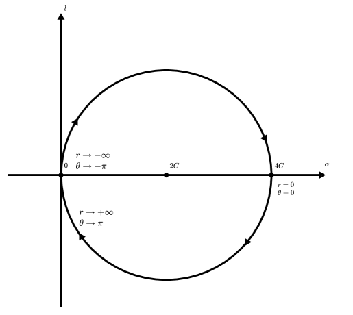
Figure 1: Phase diagram for the case $R^{2}-4C^{2}=0.$ When $r\longrightarrow-\infty,$ $\alpha,l\longrightarrow 0$ and $\theta\longrightarrow-\pi.$ When $r\longrightarrow+\infty,$ $\alpha,l\longrightarrow 0$ and $\theta\longrightarrow+\pi.$

particular, from the conserved quantity (6.9), we see that this is the solution that we obtain to the system (6.8) together with the initial conditions

$$\left\{\begin{array}[]{r}\alpha\left(0\right)=4C\\ l\left(0\right)=0\end{array}\right..$$ (6.19)

If $L$ is non-compact, then this solution is defined globally. On the other hand, if $L\cong S^{1},$ then this solution is not globally defined, and exists only locally.

6.1.2 $R^{2}-4C^{2}>0$

If $R^{2}-4C^{2}>0$, then define the quantity $Q$ via

$$Q^{2}=R^{2}-4C^{2}.$$ (6.20)

Then from (6.10), we obtain a solution

$$\alpha=\frac{4A_{0}Q^{2}e^{-rQ}}{\left(A_{0}e^{-rQ}-4C\right)^{2}+4Q^{2}}$$ (6.21)

where $A_{0}$ is a constant that depends on initial conditions. Note that an equivalent solution is obtained by taking $r\longrightarrow-r$. From (6.21) we easily obtain solutions for $l$ and $\theta$:

$$l = \frac{Q\left(A_{0}^{2}e^{-2rQ}-4R^{2}\right)}{\left(A_{0}e^{-rQ}-4C\right)^{2}+4Q^{2}}$$ (6.22a)

$$\theta = 2\arctan\left(\frac{1}{2Q}\left(4C-A_{0}e^{-rQ}\right)\right)$$ (6.22b)

Figure 2 shows for this solution in the $\alpha-l$ space. Similarly as in the case for $R^{2}-4C^{2}=0,$ these solutions are only defined globally for non-compact $L.$ Taking $A_{0}=\pm 2R,$ and translating the $r$ coordinate, the solutions (6.22) are hence solutions of (6.8) with the initial conditions

$$\left\{\begin{array}[]{r}\alpha\left(r_{0}\right)=2C\pm R\\ l\left(r_{0}\right)=0\end{array}\right.$$ (6.23)

for some $r_{0}\in\mathbb{R}$ and $\left|R\right|>2\left|C\right|$.

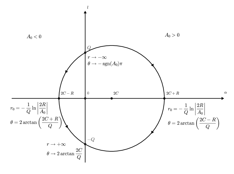
Figure 2: Phase diagram for the case $Q^{2}=R^{2}-4C^{2}>0.$ The sign of $\alpha$ in the solution depends on the sign of the constant $A_{0}$. When $r\longrightarrow-\infty,$ $\alpha\longrightarrow 0$ and $l\longrightarrow Q.$ When $r\longrightarrow+\infty$, $\alpha\longrightarrow 0$ and $l\longrightarrow-Q$.

In the case when $C=0$, then $R=$ $Q$, so setting $b=-Q\ \$and $c=-\frac{A_{0}}{2Q}$ we obtain

$$l = b\frac{1-c^{2}e^{2br}}{1+c^{2}e^{2br}}$$

$$\theta = 2\arctan\left(ce^{br}\right)$$

This is precisely the solution that was obtained by Karigiannis, McKay and Tsui in [19] for the negative Laplacian flow soliton in this setting.

6.1.3 $R^{2}-4C^{2}<0$

Now suppose $R^{2}-4C^{2}$ is negative. Then we let

$$Q^{2}=4C^{2}-R^{2}$$

The solution for $\alpha$ is then

$$\alpha=\frac{4Q^{2}A_{0}}{8CA_{0}-\left(4R^{2}+A_{0}^{2}\right)\cos rQ-i\left(4R^{2}-A_{0}^{2}\right)\sin rQ}$$

Since we need $\alpha$ to be real, we have to have $A_{0}^{2}=\pm 4R^{2}.$ Hence, we get the following possible solutions

$$\alpha=\left\{\begin{array}[]{r}\frac{Q^{2}}{2C\pm R\cos rQ}\ \ \text{if }A_{0}^{2}=+4R^{2}\\ \frac{Q^{2}}{2C\pm R\sin rQ}\ \text{if }A_{0}^{2}=-4R^{2}\end{array}\right.$$ (6.24)

Note that these solutions are equivalent under diffeomorphisms of $L$ - so by redefining $r$ we can move from one solution to another. Therefore, without loss of generality we will only consider the solution

$$\alpha=\frac{Q^{2}}{2C+R\cos rQ}$$ (6.25)

From (6.25) we obtain the corresponding solutions for $l$ and $\theta$:

$$l = \frac{QR\sin\left(rQ\right)}{2C+R\cos\left(rQ\right)}$$ (6.26a)

$$\theta = 2\arctan\left(\frac{2C-R}{Q}\tan\left(\frac{1}{2}rQ\right)\right)$$ (6.26b)

Given the freedom to redefine the coordinate $r$, the solutions of the form (6.26) are solutions to the system (6.8) together with the initial conditions

$$\left\{\begin{array}[]{r}\alpha\left(r_{0}\right)=2C\pm R\\ l\left(r_{0}\right)=0\end{array}\right.$$ (6.27)

for some $r_{0}\in\mathbb{R}$ and $\left|R\right|<2\left|C\right|$. Figure 3 shows the phase diagram for this solution with $r_{0}=0$.

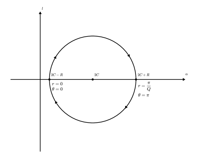
Figure 3: Phase diagram for the case $4C^{2}-R^{2}>0.$

The solutions (6.26) are of particular interest because they are periodic and thus given appropriate initial conditions they are globally defined when the manifold $M^{7}=L\times M^{6}$ is compact - in particular when $L=S^{1}.$ Suppose $r$ is a coordinate on $S^{1}$, taking values in $[0,2\pi).$ Then, if $Q=2n$ for some integer $n$, then the solutions (6.26) are periodic, and are hence well-defined on $S^{1}$. Note that when $\frac{1}{2}rQ$ is equal to a half-integer multiple of $\pi,$ there is a discontinuity in the solution for $\theta$, with $\theta\longrightarrow\pi$ when $\frac{1}{2}rQ$ approaches a half-integer multiple of $\pi$ from the left, and $\theta\longrightarrow-\pi$ when taking the limit from the right. However $\theta$ is itself defined up to an integer multiple of $2\pi$, so the actual solution for the $G_{2}$-structure is still continuous and moreover smooth.

6.2 Nearly Kähler case

Let us now consider the case when the $6$-dimensional base manifold is nearly Kähler. As before, let $k=2$ and $G=1.$ Then, the soliton equation (6.6) become

$$l^{\prime} = -\alpha^{2}+3\beta^{2}+12\alpha\beta+2C\alpha-\mu$$ (6.28a)

$$\left(\alpha-6\beta\right)^{\prime} = \alpha l$$ (6.28b)

$$\frac{\beta^{\prime}l}{\alpha+\beta} = 9\beta^{2}-\alpha\beta+2C\beta+\mu$$ (6.28c)

This system is very difficult to analyze, because it has no apparent symmetries or conserved quantities. We can however look at special solutions where at least one of the variables $\alpha,\beta,l$ is constant.

Theorem 6.5

The only solutions of the system (6.28) with at least one of the variables $\alpha,\beta,l$ constant are

1. $\alpha=0,\ \beta=0,~{}l^{\prime}=-\mu,$ for arbitrary $\mu$

2. $\alpha=0,$ $\mu=-9\beta^{2}-2C\beta,$ $l^{\prime}=2\beta\left(6\beta+C\right),$ for arbitrary constant $\beta$

3. $\alpha=0,$ $\beta=-\frac{1}{6}C,\ \mu=\frac{1}{12}C^{2},$ $l$ arbitrary

4. $l=0,\ \alpha=\frac{1}{10}C\pm\frac{1}{10}\sqrt{C^{2}-10\mu}$, $\beta=-\alpha$  for $\mu\leq\frac{C^{2}}{10}$

5. $l=0,\ \alpha=4\sqrt{3\mu}+2C,\beta=\frac{1}{3}\sqrt{3\mu}\$for $\mu\geq 0$

Proof. We will consider different cases where $\beta,$ $\alpha$ or $l$ are constant.

Constant $\beta$

Suppose $\beta^{\prime}=0$. Then, (6.28c) becomes

$$\left(9\beta^{2}-\alpha\beta+2C\beta+\mu\right)\left(\alpha+\beta\right)=0$$ (6.29)

From this, either $\mu=0$ and $\beta=0,$ or $\alpha$ must also be constant and must either satisfy $9\beta^{2}-\alpha\beta+2C\beta+\mu=0$ or $\alpha+\beta=0$. In the first case, the equations reduce to (6.8) - the equations we had in the Calabi-Yau case. Now however, since $\lambda\neq 0$, in order to have $\beta=\frac{\lambda\sin\theta}{h}=0$, we must have $\sin\theta=0.$ In particular, $\theta$ must be constant. However, from Theorem 6.4, this is true if and only if $C=0$ and we have a trivial solution. Therefore, for a non-trivial solution, $\alpha$ has to be constant. From (6.28b), this however implies that $\alpha l=0.$ The case $l=0$ will be considered below. Suppose $\alpha=0$. Then, from (6.28a) we have

$$l^{\prime}=3\beta^{2}-\mu$$

From (6.29), either $\beta$ is also zero, and $l^{\prime}=-\mu$ or $\mu=-9\beta^{2}-2C\beta,$ so that

$$l^{\prime}=2\beta\left(6\beta+C\right).$$

Thus, we obtain solutions $1$ and $2$.

Constant $\alpha$

Suppose $\alpha^{\prime}=0$. Then, the equations (6.28) become

$$l^{\prime} = -\alpha^{2}+3\beta^{2}+12\alpha\beta+2C\alpha-\mu$$ (6.30a)

$$\beta^{\prime} = -\frac{1}{6}\alpha l$$ (6.30b)

$$\beta^{\prime}l = \left(9\beta^{2}-\alpha\beta+2C\beta+\mu\right)\left(\alpha+\beta\right)$$ (6.30c)

We already considered the case of constant $\beta$, so suppose $\alpha\neq 0\$and $l\neq 0$. From equations (6.30a) and (6.30b), we find a conserved quantity $F,$ given by

$$\alpha l^{2}+12\left(\beta^{3}+6\alpha\beta^{2}-\left(\alpha^{2}-2C\alpha+\mu\right)\beta\right)=F$$

while, from equations (6.30b) and (6.30c), we find

$$\alpha l^{2}+6\left(9\beta^{2}-\alpha\beta+2C\beta+\mu\right)\left(\alpha+\beta\right)=0.$$

From these two equations, we find that $\beta$ satisfies a cubic equation with constant coefficients, and hence must also be constant. Therefore, we do not get any new solutions in this case.

Constant $l$

Suppose $l^{\prime}=0$. Then, the equation (6.28a) becomes

$$-\alpha^{2}+3\beta^{2}+12\alpha\beta+2C\alpha-\mu=0$$ (6.31)

Differentiating this, we find

$$\alpha^{\prime}\left(-\alpha+6\beta+C\right)+3\beta^{\prime}\left(\beta+2\alpha\right)=0$$

Substituting (6.28b), we get

$$\alpha l\left(-\alpha+6\beta+C\right)+3\beta^{\prime}\left(13\beta+2C\right)=0$$

Now using (6.28c), we get another polynomial equation for $\alpha$ and $\beta$

$$\alpha l^{2}\left(-\alpha+6\beta+C\right)+3\left(9\beta^{2}-\alpha\beta+2C\beta+\mu\right)\left(\alpha+\beta\right)\left(13\beta+2C\right)=0$$ (6.32)

Therefore, $\alpha$ and $\beta$ satisfy the polynomial equations (6.31) and (6.32). By explicit calculations (using Maple) it can be shown that $\alpha$ and $\beta$ must be constants that depend on $C,l$ and $\mu.$ However, it means that in equation (6.28b), either $\alpha=0$ or $l=0.$ Suppose $\alpha=0$. Then, from (6.28a) we get that

$$\beta^{2}=\frac{\mu}{3}$$

So $\beta^{\prime}=0,$ and thus from (6.28c), we get

$$\left(9\beta^{2}+2C\beta+\mu\right)\beta=0$$

So either $\beta=0,$ which is a case we already covered in (6.37), or

$$\beta=-\frac{1}{6}C,\ \mu=\frac{1}{12}C^{2}$$ (6.33)

Note that in these cases $l$ is an arbitrary constant.

The other possibility is that $l=0$. So suppose $\alpha\neq 0$. In this case, $\alpha$ and $\beta$ have to satisfy (6.31) and

$$\left(9\beta^{2}-\alpha\beta+2C\beta+\mu\right)\left(\alpha+\beta\right)=0$$ (6.34)

Then either $\beta=-\alpha$, where $\alpha$ satisfies

$$10\alpha^{2}-2C\alpha+\mu=0,$$

which gives solution 4, or

$$9\beta^{2}-\alpha\beta+2C\beta+\mu=0.$$ (6.35)

Note that the equations (6.31) and (6.35) are equivalent if $\beta=-\alpha$, but we already considered this case. Suppose $\beta\neq 0$. Then, from (6.35),

$$\alpha=\frac{1}{\beta}\left(\mu+2C\beta+9\beta^{2}\right)$$

Using this we find that (6.31) simplifies to

$$\left(\mu-3\beta^{2}\right)\left(10\beta^{2}+2C\beta+\mu\right)=0$$

and hence

$$\alpha\left(\mu-3\beta^{2}\right)\left(\alpha+\beta\right)=0.$$

We have already considered the cases $\alpha=0$ and $\alpha+\beta=0$, hence $\beta^{2}=\frac{\mu}{3}$. Thus we get solution 5. If however, $\beta=0$, then equation (6.35) forces $\mu=0$, and hence from (6.31) $\alpha=0$ or $\alpha=2C$. These cases are however already covered. Therefore this exhausts all the possible solutions.   

Remark 6.6

Recall from (3.29) that the $\tau_{27}$ component of the torsion is proportional to $\alpha+\beta$. Therefore, in Proposition 6.5, the solution 5 always has $\tau_{27}=0,$ since $\alpha+\beta=0.$ Therefore, this solution corresponds to a nearly parallel $G_{2}$ structure with only the $\tau_{1}$ torsion component being non-zero. Since in this solution the only restriction on $\mu$ is that $\mu\leq\frac{C^{2}}{10}$ we may have solutions of different kinds - shrinking solutions ($\mu$ negative), expanding solutions ($\mu$ positive), and steady solutions ($\mu=0$). Similarly, in solution 5, we can get $\alpha+\beta=0$ if $C$ is negative and

$$\mu=\frac{12}{169}C^{2}.$$

So for this value of $\mu$ we obtain another nearly parallel solution. However this time, these are all expanding solutions (except the trivial steady case when $C=0$). Moreover, by fixing

$$\mu=\frac{1}{3}C^{2}$$

we obtain $\alpha-6\beta=0.$ This gives $\tau_{1}=0$, and a non-zero $\tau_{27}$ - hence this soliton solution is a $G_{2}$-structure of pure type $\mathbf{27}.$

A special simple solution is $\alpha=\beta=0$. Note that in this case, the torsion vanishes, and we have a torsion-free $G_{2}$-structure. Then, the first equation just becomes

$$l^{\prime}=-\mu$$ (6.36)

From the definition of $\beta,$ we find that $\sin\theta=0$, so $\theta=0$ or $\pi$. However from $\gamma=0$, we also have $h^{\prime}=-\lambda\cos\theta.$ Thus we have the following solutions:

$$\left\{\begin{array}[]{c}\theta=0,\ \ h=-\lambda r+h_{0},\ l=-\mu r+l_{0}\\ \theta=\pi,\ \ h=\lambda r+h_{0},\ l=-\mu r+l_{0}\end{array}\right.$$ (6.37)

These are precisely the solutions also obtained in [19].

Consider now another special case where $l$ is constant. It then turns out that if $l$ is constant, then necessarily, either $l=0$ or $\mu$ has take a particular value that depends on $C$. These cases then cover all the remaining exact solutions of the corresponding system that were found in [19], as well as additional solutions.

Proposition 6.5 gives us the critical points of the equations (6.28), however it can be easily seen that linearizations at these critical points are degenerate, and therefore do not provide much information about the full system.

References

- [1] J. Baez, The Octonions, Bull. Amer. Math. Soc. (N.S.) 39 (2002) 145–205.
- [2] R. L. Bryant, Metrics with exceptional holonomy, Ann. of Math. (2) 126 (1987), no. 3 525–576.
- [3] R. L. Bryant, Some remarks on G_2-structures, in Proceedings of Gökova Geometry-Topology Conference 2005, pp. 75–109, Gökova Geometry/Topology Conference (GGT), Gökova, 2006. math/0305124.
- [4] R. L. Bryant and F. Xu, Laplacian Flow for Closed -Structures: Short Time Behavior, 1101.2004.
- [5] S. Chiossi and S. Salamon, The intrinsic torsion of and structures, in Differential geometry, Valencia, 2001, pp. 115–133. World Sci. Publ., River Edge, NJ, 2002.
- [6] R. Cleyton and S. Ivanov, Conformal equivalence between certain geometries in dimension 6 and 7, Math. Res. Lett. 15 (2008), no. 4 631–640 [math/0607487].
- [7] R. Cleyton and S. Ivanov, Curvature decomposition of -manifolds, J. Geom. Phys. 58 (2008), no. 10 1429–1449.
- [8] M. Fernández and A. Gray, Riemannian manifolds with structure group , Ann. Mat. Pura Appl. (4) 132 (1982) 19–45 (1983).
- [9] T. Friedrich, Nearly Kähler and nearly parallel -structures on spheres, Arch. Math. (Brno) 42 (2006), no. suppl. 241–243.
- [10] A. Gray, The structure of nearly Kähler manifolds, Math. Ann. 223 (1976), no. 3 233–248.
- [11] S. Grigorian, Moduli spaces of G2 manifolds, Rev. Math. Phys. 22 (2010), no. 9 1061–1097 [0911.2185].
- [12] S. Grigorian, Deformations of G2-structures with torsion, 1108.2465.
- [13] S. Grigorian, Short-time behaviour of a modified Laplacian coflow of G2-structures, Adv. Math. 248 (2013) 378–415 [1209.4347].
- [14] N. J. Hitchin, The geometry of three-forms in six and seven dimensions, J. Differential Geom. 55 (2000), no. 3 547–576 [math/0010054].
- [15] N. J. Hitchin, The geometry of three-forms in six dimensions, J. Differential Geom. 55 (2000), no. 3 547–576 [math/0010054].
- [16] D. D. Joyce, Compact manifolds with special holonomy. Oxford Mathematical Monographs. Oxford University Press, 2000.
- [17] S. Karigiannis, Deformations of G_2 and Spin(7) Structures on Manifolds, Canadian Journal of Mathematics 57 (2005) 1012 [math/0301218].
- [18] S. Karigiannis, Flows of -Structures, I, Q. J. Math. 60 (2009), no. 4 487–522 [math/0702077].
- [19] S. Karigiannis, B. McKay and M.-P. Tsui, Soliton solutions for the Laplacian coflow of some -structures with symmetry, Differential Geom. Appl. 30 (2012), no. 4 318–333 [1108.2192].
- [20] A. Moroianu, P.-A. Nagy and U. Semmelmann, Unit Killing vector fields on nearly Kähler manifolds, Internat. J. Math. 16 (2005), no. 3 281–301.
- [21] H. Weiss and F. Witt, Energy functionals and soliton equations for -forms, Ann. Global Anal. Geom. 42 (2012), no. 4 585–610 [1201.1208].
- [22] H. Weiss and F. Witt, A heat flow for special metrics, Adv. Math. 231 (2012), no. 6 3288–3322 [0912.0421].
- [23] F. Xu and R. Ye, Existence, Convergence and Limit Map of the Laplacian Flow, 0912.0074.