Halo/Galaxy Bispectrum with Equilateral-type Primordial Trispectrum

Abstract

We investigate the effect of equilateral-type primordial trispectrum on the halo/galaxy bispectrum. We consider three types of equilateral primordial trispectra which are generated by quartic operators naturally appeared in the effective field theory of inflation and can be characterized by three non-linearity parameters, $g_{\rm NL}^{\dot{\sigma}^{4}}$, $g_{\rm NL}^{\dot{\sigma}^{2}(\partial\sigma)^{2}}$, and $g_{\rm NL}^{(\partial\sigma)^{4}}$. Recently, constraints on these parameters have been investigated from CMB observations by using WMAP9 data. In order to consider the halo/galaxy bispectrum with the equilateral-type primordial trispectra, we adopt the integrated Perturbation Theory (iPT) in which the effects of primordial non-Gaussianity are wholly encapsulated in the linear primordial polyspectrum for the evaluation of the biased polyspectrum. We show the shapes of the halo/galaxy bispectrum with the equilateral-type primordial trispectra, and find that the primordial trispectrum characterized by $g_{\rm NL}^{\dot{\sigma}^{4}}$ provides the same scale-dependence as the gravity-induced halo/galaxy bispectrum. Hence, it would be difficult to obtain the constraint on $g_{\rm NL}^{\dot{\sigma}^{4}}$ from the observations of the halo/galaxy bispectrum. On the other hand, the primordial trispectra characterized by $g_{\rm NL}^{\dot{\sigma}^{2}(\partial\sigma)^{2}}$ and $g_{\rm NL}^{(\partial\sigma)^{4}}$ provide the common scale-dependence which is different from that of the gravity-induced halo/galaxy bispectrum on large scales. Hence future observations of halo/galaxy bispectrum would give constraints on the non-linearity parameters, $g_{\rm NL}^{\dot{\sigma}^{2}(\partial\sigma)^{2}}$ and $g_{\rm NL}^{(\partial\sigma)^{4}}$ independently from CMB observations and it is expected that these constraints can be comparable to ones obtained by CMB.

I Introduction

The primordial non-Gaussianity provide crucial information on the interaction structure of inflation (for a review, see Bartolo:2004if ). At present, a most stringent constraint on primordial non-Gaussianity is provided by Planck collaboration Ade:2015ava and it implies no evidence of non-Gaussianity. Although the resultant constraint has almost approached the observational limit predicted by ideal observations, it is still rather weak from a particle physics point of view. Therefore, it would be very interesting to try further constraining the non-Gaussianity based on the information other than CMB.

For this purpose, it has been recently noticed that large-scale halo/galaxy distributions provide a distinct information on the primordial non-Gaussianity. Especially, in the presence of local-type primordial non-Gaussianity, it has been shown that the halo/galaxy power spectrum is enhanced on large scales (so-called scale-dependent bias), which is helpful to impose the constraint on the primordial non-Gaussianity (e.g., Dalal:2007cu ; Slosar:2008hx ; Matarrese:2008nc ). Although the current constraints derived from the scale-dependent bias is still weaker than the one from CMB Giannantonio:2013uqa , from the future observational projects such as DES Abbott:2005bi , BigBoss Schlegel et al.(2011) , LSST LSST Science Collaboration et al.(2009) , EUCLID 2011arXiv1110.3193L and HSC/PFS (Sumire) 2014PASJ…66R…1T , it is expected that we can get the constraint $\Delta f_{\rm NL}^{\rm local}\sim\mathcal{O}(0.1)$ Yamauchi:2014ioa .

The influence of scale-dependent bias sourced by the primordial non-Gaussianity appears not only in the halo/galaxy power spectrum but also in the halo/galaxy bispectrum and other polyspectra. Although it is well known that the late-time nonlinear gravitational evolution also gives the non-Gaussianity, if the amplitude of primordial non-Gaussianity is sufficiently large, the halo/galaxy bispectrum sourced by the primordial non-Gaussianity has a different scale dependence from the non-linear gravitational evolution and it can dominate on large scales Sefusatti:2007ih ; Jeong:2009vd ; Sefusatti:2009qh ; Baldauf:2010vn ; Nishimichi:2009fs ; Yokoyama:2013mta ; Tasinato:2013vna ; Gil-Marin:2014pva ; Tellarini:2015faa . Especially, when we consider the higher order local-type primordial non-Gaussianity, by combining the analysis of the halo/galaxy power spectrum with the bispectrum it is expected that we could get much tighter constraint on the primordial non-Gaussianity. Another important fact with the halo/galaxy bispectrum is that the amplitude of the contribution sourced by the equilateral-type primordial bispectrum is also shown to be enhanced on large scales Sefusatti:2007ih ; Sefusatti:2009qh ; Yokoyama:2013mta , which does not give an enhancement in the halo/galaxy power spectrum.

Regardless of these works, compared with the analysis of CMB, the one of LSS has not covered another important class of primordial non-Gaussianity, that is, the trispectra generated in theoretical models which produce the equilateral-type bispectrum, which we call equilateral-type trispectra from now on. This is because the shapes of primordial trispectra of this class strongly depend on the theoretical models and they are generically much more complicated than those of the local-type trispectra. Recently, however, Ref. Smith:2015uia has investigated an optimal analysis of the such kind of equilateral-type trispectra by making use of CMB observations (for the earlier works to obtain the constraints on the equilateral-type trispectra based on CMB observations, see Refs. Regan:2010cn ; Mizuno:2010by ; Fergusson:2010gn ; Izumi:2011di ; Regan:2013jua ). For the analysis they introduce three new non-linearity parameters, $g_{\rm NL}^{\dot{\sigma}^{4}}$, $g_{\rm NL}^{\dot{\sigma}^{2}(\partial\sigma)^{2}}$, and $g_{\rm NL}^{(\partial\sigma)^{4}}$, which respectively represent the amplitudes of the primordial trispectra that correspond to quartic operators of the form $\dot{\sigma}^{4}$, $\dot{\sigma}^{2}(\partial\sigma)^{2}$, and $(\partial\sigma)^{4}$ in the effective field theory of inflation (we will show the detailed forms of these trispectra later in section IV). The reason that only these three trispectra have been considered is that their forms are relatively simple and they have natural theoretical origin in the sense that they are shown to be generated by general $k$-inflation Huang:2006eha ; Arroja:2009pd ; Chen:2009bc and the effective field theory of inflation Senatore:2010jy ; Senatore:2010wk .

Following Ref. Smith:2015uia , in this paper, we investigate the effect of these three equilateral-type primordial trispectra on the halo/galaxy bispectrum and see if we can get constraints on these trispectra from the future LSS observations independently from those from CMB. For this purpose, we adopt the integrated Perturbation Theory (iPT) Matsubara:2011ck which enables us to connect the halo/galaxy clustering with the initial matter density field and incorporate the non-local biasing effect in a straightforward manner Yokoyama:2013mta ; Matsubara:2012nc ; Matsubara:2013ofa ; Yokoyama:2012az ; Sato:2013qfa . Furthermore, it is worth mentioning that in iPT, we do not rely on the approximations like the peak-background split and the peak formalism.

This paper is organized as follows. In Sec. II, we begin by presenting a general formula for the halo/galaxy bispectrum in the presence of the primordial bispectrum and trispectrum in terms of iPT. In Sec. III, we show that while the effect of the equilateral-type primordial bispectrum does not appear in the halo/galaxy power spectrum, it appears in the halo/galaxy bispectrum. For the analysis, we estimate the amplitude of each contribution based on the the equilateral configuration where the signal becomes maximum. Then, we investigate the effect of the equilateral-type trispectra mentioned above on the halo/galaxy bispectrum and show that two of them, $T_{\Phi}^{\dot{\sigma}^{2}(\partial\sigma)^{2}}$ and $T_{\Phi}^{(\partial\sigma)^{4}}$ can give the dominant contribution on very large scales, while $T_{\Phi}^{\dot{\sigma}^{4}}$ gives the same scale-dependence as the one induced by the nonlinearity of the gravitational evolution in Sec. IV. In the same section, we also consider the shape-dependence of the halo/galaxy bispectrum to distinguish the effects by the equilateral-type bispectrum from the equilateral-type trispectra $T_{\Phi}^{\dot{\sigma}^{2}(\partial\sigma)^{2}}$ and $T_{\Phi}^{(\partial\sigma)^{4}}$ which provide the common scale-dependence on large scales for the equilateral configuration. Sec. V is devoted to summary. In our numerical works, through this paper, we adopt the best fit cosmological parameters taken from Planck Planck:2015xua unless specifically mentioned.

II Halo/Galaxy spectra with primordial non-Gaussianity

In this section, we briefly review the formula for the power- and bi-spectra of galaxies and halos with primordial non-Gaussianity based on the integrated perturbation theory (iPT). In Sec. II.1, we first present the general expressions for the power and bispectrum. We keep the terms giving leading contributions up to the one-loop order in iPT. We then derive the concrete expressions of the multi-point propagators in the large-scale limit in Sec. II.2, which will be the important building blocks to study the scale-dependent behavior of the power and bispectrum on large scales.

II.1 Halo/Galaxy Power spectrum and Bispectrum from integrated perturbation theory

We begin by defining the power- and bi-spectra of biased objects (halos/galaxies), $P_{X}$ and $B_{X}$:

$$\langle\delta_{X}({\bf k})\delta_{X}({\bf k}^{\prime}))\rangle \equiv (2\pi)^{3}\delta^{(3)}({\bf k}+{\bf k}^{\prime})P_{X}(k)\,,$$ (1)

$$\langle\delta_{X}({\bf k}_{1})\delta_{X}({\bf k}_{2})\delta_{X}({\bf k}_{3})\rangle \equiv (2\pi)^{3}\delta^{(3)}({\bf k}_{1}+{\bf k}_{2}+{\bf k}_{3})B_{X}({\bf k}_{1},{\bf k}_{2},{\bf k}_{3})\,,$$ (2)

where the quantity $\delta_{X}$ is a Fourier transform of the number density field of the biased objects. In iPT, the perturbative expansion of the statistical quantities such as power- and bi-spectra of biased objects are composed of the multi-point propagators and the polyspectra of the linear density field $\delta_{L}$.

The definition of the $(n+1)$-point propagator of the biased objects $\Gamma^{(n)}_{X}$ is given by Matsubara:2011ck

$$\left\langle\frac{\delta^{n}\delta_{X}({\bf k})}{\delta\delta_{\rm L}({\bf k}_{1})\delta\delta_{\rm L}({\bf k}_{2})\cdots\delta\delta_{\rm L}(({\bf k}_{n})}\right\rangle=(2\pi)^{3-3n}\delta({\bf k}_{1}+{\bf k}_{2}+\cdots+{\bf k}_{n})\Gamma^{(n)}_{X}({\bf k}_{1},{\bf k}_{2},\cdots,{\bf k}_{n})\,,$$ (3)

and it represents the influence on $\delta_{X}$ due to the infinitesimal variation for the initial density field $\delta_{L}$ like non-linear gravitational evolution, non-local bias, redshift space distortion etc. In Sec. II.2, we will show the concrete expression of the 2- and 3-point propagators in the large-scale limit which play important roles in this paper.

On the other hand, the power-, bi- and tri-spectra of the linear density field $P_{\rm L}$, $B_{\rm L}$ and $T_{\rm L}$ are defined by

$$\langle\delta_{\rm L}({\bf k})\delta_{\rm L}({\bf k}^{\prime})\rangle = (2\pi)^{3}\delta({\bf k}+{\bf k}^{\prime})P_{\rm L}(k)\,,$$

$$\langle\delta_{\rm L}({\bf k}_{1})\delta_{\rm L}({\bf k}_{2})\delta_{\rm L}({\bf k}_{3})\rangle = (2\pi)^{3}\delta({\bf k}_{1}+{\bf k}_{2}+{\bf k}_{3})B_{\rm L}({\bf k}_{1},{\bf k}_{2},{\bf k}_{3})\,,$$

$$\langle\delta_{\rm L}({\bf k}_{1})\delta_{\rm L}({\bf k}_{2})\delta_{\rm L}({\bf k}_{3})\delta_{\rm L}({\bf k}_{4})\rangle = (2\pi)^{3}\delta({\bf k}_{1}+{\bf k}_{2}+{\bf k}_{3}+{\bf k}_{4})T_{\rm L}({\bf k}_{1},{\bf k}_{2},{\bf k}_{3},{\bf k}_{4})\,.$$ (4)

It is worth mentioning that the linear density field $\delta_{\rm L}$ is related to the primordial curvature perturbation $\Phi$ through the function $\mathcal{M}(k)$:

$$\delta_{L}(k)=\mathcal{M}(k)\Phi(k);\;\;\;\;{\mathcal{M}}(k)=\frac{2}{3}\frac{D(z)}{D(z_{*})(1+z_{*})}\frac{k^{2}T(k)}{H_{0}^{2}\Omega_{m0}}\,,$$ (5)

where $T(k)$, $D(z)$, $H_{0}$ and $\Omega_{m0}$ are the transfer function, the linear growth factor, the Hubble parameter at present epoch, and the matter density parameter, respectively. $z_{*}$ denotes an arbitrary redshift at the matter-dominated era. For the concrete form of the transfer function and the linear growth factor, we use the ones adopted in Chongchitnan:2010xz and Linder:2005in , respectively. Furthermore, because of the finite resolution of any observation, the density field always requires the procedure of the smoothing over some length scale $R$. For the smoothing, we use the window function $W(kR)$ which is the spherical top-hat function of $R$,

$$W(kR)=3\left[\frac{\sin(kR)}{(kR)^{3}}-\frac{\cos(kR)}{(kR)^{2}}\right]\,,$$ (6)

in Fourier space. It is also useful to define the mass scale $M$

$$M\equiv\frac{4}{3}\pi R^{3}\rho_{m}\simeq 1.16\times 10^{12}\Omega_{m0}\left(\frac{R}{h^{-1}{\rm Mpc}}\right)^{3}h^{-1}M_{\odot}\,,$$ (7)

which is regarded as the mass of matter enclosed by the top-hat window.

With the relation (5), the linear power spectrum is expressed in terms of that of the primordial curvature perturbation as

$$P_{\rm L}(k)=\mathcal{M}(k)^{2}P_{\Phi}(k)\,,$$ (8)

with

$$\langle\Phi({\bf k})\Phi({\bf k}^{\prime})\rangle=(2\pi)^{3}\delta({\bf k}+{\bf k}^{\prime})P_{\Phi}(k)\,,$$ (9)

where we assume the scale-invariant primordial power spectrum, that is, $P_{\Phi}(k)\propto k^{-3}$, for simplicity. We can define the variance of density fluctuations smoothed on scale $R$ by

$$\sigma_{R}^{2}\equiv\frac{1}{2\pi^{2}}\int_{0}^{\infty}dkk^{2}W(kR)^{2}\mathcal{M}(k)^{2}P_{\Phi}\,,$$ (10)

and we choose the normalization of the primordial power spectrum so that it gives

$$\sigma_{8}=\sigma(R=8h^{-1}{\rm Mpc})=0.815\,,$$ (11)

which is the value of $\sigma_{8}$ reported by Planck collaboration Planck:2015xua .

In terms of the multi-point propagators and the linear polyspectra introduced above, the power spectrum of the biased objects can be written as

$$P_{X}(k)=P_{0}+P_{\rm bis}+\cdots\,.$$ (12)

with

$$P_{0} = \left[\Gamma_{X}^{(1)}({\bf k})\right]^{2}P_{\rm L}(k)\,,$$ (13)

$$P_{\rm bis} = \Gamma_{X}^{(1)}({\bf k})\int\frac{d^{3}p}{(2\pi)^{3}}\Gamma_{X}^{(2)}({\bf p},{\bf k}-{\bf p})B_{\rm L}(\bf{k},-\bf{p},-{\bf k}+{\bf p})\,.$$ (14)

Here we have considered the perturbative expansion up to the one-loop order in iPT. Up to the one-loop order in iPT, the contribution from the primordial trispectrum does not appear. It appears at the two-loop order. However, as shown later, in case with the equilateral-type non-Gaussianity, the one-loop order contribution given by Eq. (14), which is induced by the primordial bispectrum, is not so significant and it is expected that two-loop order contribution related with the primordial trispectrum would be much suppressed. Hence, here, for the halo/galaxy power spectrum we neglect the contribution from the equilateral-type primordial trispectrum.

Similarly, the bispectrum of the biased objects can be written as

$$B_{X}({\bf k}_{1},{\bf k}_{2},{\bf k}_{3})=B_{\rm grav}+B_{\rm bis}+B_{\rm tris}+\cdots\,,$$ (15)

with

$$B_{\rm grav} = \left[\Gamma^{(1)}_{X}({\bf k}_{1})\Gamma^{(1)}_{X}({\bf k}_{2})\Gamma^{(2)}_{X}(-{\bf k}_{1},-{\bf k}_{2})P_{\rm L}(k_{1})P_{\rm L}(k_{2})+2\;{\rm perms.}\right]\,,$$ (16)

$$B_{\rm bis} = \Gamma^{(1)}_{X}({\bf k}_{1})\Gamma^{(1)}_{X}({\bf k}_{2})\Gamma^{(1)}_{X}({\bf k}_{3})B_{\rm L}({\bf k}_{1},{\bf k}_{2},{\bf k}_{3})\,,$$ (17)

$$B_{\rm tris} = \frac{1}{2}\Gamma^{(1)}_{X}({\bf k}_{1})\Gamma^{(1)}_{X}({\bf k}_{2})\int\frac{d^{3}p}{(2\pi)^{3}}\Gamma^{(2)}_{X}({\bf p},{\bf k}_{3}-{\bf p})T_{\rm L}({\bf k}_{1},{\bf k}_{2},{\bf p},{\bf k}_{3}-{\bf p})+2\;{\rm perms.}\,.$$ (18)

Again, we have considered the perturbative expansion up to the one-loop order in iPT and we find that for the halo/galaxy bispectrum the contribution from the primordial trispectrum appears at the one-loop order.

In Fig. 1, diagrammatic representation of each term in Eqs. (12) and (15) is shown. A double solid line connected with a grey circle indicate the multi-point propagator of biased objects $\Gamma^{(n)}_{X}$ while a crossed circle glued to multiple single solid lines indicate the correlator of the initial linear density field.

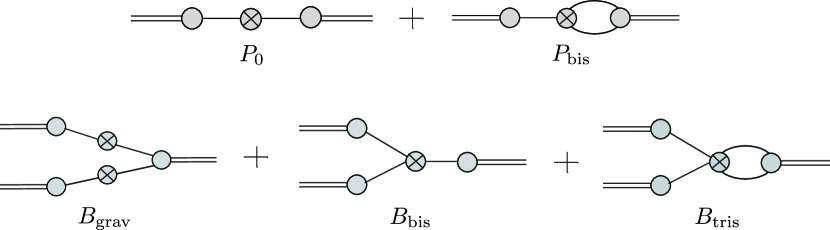
Figure 1: Diagrammatic representation of each term in Eqs. (12) (upper) and (15) (lower).

II.2 Multi-point propagators in the large-scale limit

The multi-point propagator $\Gamma^{(n)}_{X}$ is defined as a fully non-perturbative quantity and it is difficult to evaluate it rigorously. But we know that the halo/galaxy polyspectra are generically dominated by the non-linearity of the gravitational evolution on small scales and large scales are the only window where the effect of the primordial non-Gaussianity can be significant. In such large-scale limit where the scale of interest $\sim 1/k_{i}$ is much larger than the typical scale of the formation of the collapsed object $\sim 1/p$, the perturbative treatment works well and the multi-point propagators can be simplified as

$$\Gamma^{(1)}_{X}({\bf k}) \simeq 1+c_{1}^{\rm L}(k)\,,$$

$$\Gamma^{(2)}_{X}({\bf k}_{1},{\bf k}_{2}) \simeq F_{2}({\bf k}_{1},{\bf k}_{2})+\left(1+\frac{{\bf k}_{1}\cdot{\bf k}_{2}}{k_{2}^{2}}\right)c_{1}^{\rm L}({\bf k}_{1})+\left(1+\frac{{\bf k}_{1}\cdot{\bf k}_{2}}{k_{1}^{2}}\right)c_{1}^{\rm L}({\bf k}_{2})+c_{2}^{\rm L}({\bf k}_{1},{\bf k}_{2})\,,$$ (19)

where $F_{2}$ is the second-order kernel of standard perturbation theory which is given by

$$F_{2}({\bf k}_{1},{\bf k}_{2})=\frac{10}{7}+\left(\frac{k_{2}}{k_{1}}+\frac{k_{1}}{k_{2}}\right)\frac{{\bf k}_{1}\cdot{\bf k}_{2}}{k_{1}k_{2}}+\frac{4}{7}\left(\frac{{\bf k}_{1}\cdot{\bf k}_{2}}{k_{1}k_{2}}\right)^{2}\,.$$ (20)

Due to the symmetric property of $F_{2}$, we have

$$\Gamma^{(2)}_{X}(-{\bf p},{\bf p})\simeq c_{2}^{\rm L}(-{\bf p},{\bf p})\,.$$ (21)

In Eq. (19), $c_{n}^{\rm L}$ is a renormalized bias function defined in Lagrangian space, given by

$$c_{n}^{\rm L}({\bf k}_{1},{\bf k}_{2},\cdots,{\bf k}_{n})=(2\pi)^{3n}\int\frac{d^{3}k^{\prime}}{(2\pi)^{3}}\left\langle\frac{\delta^{n}\delta^{\rm L}_{X}({\bf k}^{\prime})}{\delta\delta_{\rm L}({\bf k}_{1})\delta\delta_{\rm L}({\bf k}_{2})\cdots\delta\delta_{\rm L}(({\bf k}_{n})}\right\rangle\,,$$ (22)

where $\delta^{\rm L}_{X}$ is the number density field of biased objects in Lagrangian space.

For a simple model of non-local halo bias proposed by Ref. Matsubara:2011ck ; Matsubara:2013ofa , the renormalized bias function for halos with mass $M$ is given by

$$c_{n}^{\rm L}({\bf k}_{1},{\bf k}_{2},\cdots,{\bf k}_{n})=\frac{A_{n}(M)}{\delta^{n}_{c}}W(k_{1};M)\cdots W(k_{n};M)+\frac{A_{n-1}(M)\sigma^{n}_{M}}{\delta^{n}_{c}}\frac{d}{d\ln\sigma_{M}}\left[\frac{W(k_{1};M)\cdots W(k_{n};M)}{\sigma^{n}_{M}}\right]\,,$$ (23)

where $\delta_{c}(\simeq 1.686)$ is the so-called critical density of the spherical collapse model and $\sigma_{M}$ is the variance of density fluctuations on the mass scale $M$ defined by Eq. (7). Here, $A_{n}(M)$ is defined by

$$A_{n}(M)\equiv\sum^{n}_{j=0}\frac{n!}{j!}\delta^{j}_{c}b^{\rm L}_{j}(M)\,,$$ (24)

where $b^{\rm L}_{j}(M)$ is the $j$-th order scale-independent Lagrangian bias parameter which is constructed from the universal mass function as

$$b^{\rm L}_{j}(M)=(-\sigma_{M})^{-j}f_{\rm MF}^{-1}\frac{d^{j}}{d\nu^{j}}(f_{\rm MF}(\nu))\,.$$ (25)

Throughout the paper, we adopt Sheth-Tormen mass function Sheth:1999mn given by

$$f_{\rm ST}(\nu)=A(p)\sqrt{\frac{2}{\pi}}[1+(q\nu^{2})^{-p}]\sqrt{q}\nu e^{-q\nu^{2}/2}\,.$$ (26)

In Eq. (26), $\nu=\delta_{c}/\sigma_{M}$, $p=0.3$, $q=0.707$ and the normalization factor $A(p)=[1+\Gamma(1/2-p)/(\sqrt{\pi}2^{p})]^{-1}$.

In the large scale limit where $k_{i}\to 0$, the window function and its derivative approach $W(k_{i};R)\to 1$ and $dW(k_{i};R)/d\ln\sigma_{M}\to 0$. Therefore, the renormalized bias function, either the multi-point propagator does not have significant scale-dependence. Before closing this section, for the later convenience, it is worth mentioning that in the large-scale limit, $\mathcal{M}(k)$ appeared in Eq. (5) has a scale-dependence

$$\mathcal{M}(k)\propto k^{2}\,.$$ (27)

III Halo/Glaxy power spectrum and bispectrum with equilateral-type primordial bispectrum

In this section, based on the simple expressions for the multi-point propagators on large scales which are obtained in the previous section, we will investigate the effect of equilateral-type primordial bispectrum on the halo/galaxy power spectrum and bispectrum in Sec III.1 and III.2, in order.

III.1 Halo/Galaxy power spectrum with equilateral-type primordial bispectrum

Among the terms of the halo/galaxy power spectrum in Eq. (12), $P_{0}$ generically gives the dominant contribution on small scales, which means that any type of corrections can be significant only on large scales. Therefore, first let us see the scale-dependence of $P_{0}$ in the large-scale limit. From Eq. (13) and making use of the fact that $\Gamma^{(1)}_{X}({\bf k})$ has no scale-dependence on large scales, it is estimated as

$$P_{0} \propto \mathcal{M}(k)^{2}P_{\Phi}\propto k\,.$$ (28)

On the other hand, in the presence of the primordial bispectrum, the possible correction to $P_{X}$ is given by $P_{\rm bis}$ in Eq. (12). From Eq. (14), in the large-scale limit $P_{\rm bis}$ can be approximated as

$$P_{\rm bis} \simeq \Gamma^{(1)}_{X}({\bf k})\int\frac{d^{3}p}{(2\pi)^{3}}\Gamma^{(2)}_{X}({\bf p},-{\bf p})B_{\rm L}({\bf k},-{\bf p},{\bf p})$$ (29)

$$= \Gamma^{(1)}_{X}({\bf k})\mathcal{M}(k)\int\frac{d^{3}p}{(2\pi)^{3}}\Gamma^{(2)}_{X}({\bf p},-{\bf p})\mathcal{M}(p)^{2}B_{\Phi}({\bf k},-{\bf p},{\bf p})\,.$$

Therefore, the scale-dependence of $P_{\rm bis}$ in the large-scale limit depends on the type of primordial bispectrum.

It is well known that the effect of the local-type primordial bispectrum whose amplitude is characterized by the nonlinearity parameter, $f_{\rm NL}^{\rm local}$, appears in the halo/galaxy power spectrum on large scales. Actually, by substituting the following shape of the local-type primordial bispectrum Komatsu:2001rj ,

$$B_{\Phi}^{\rm local}({\bf k}_{1},{\bf k}_{2},{\bf k}_{3})=2f_{\rm NL}^{\rm local}\left[P_{\Phi}(k_{1})P_{\Phi}(k_{2})+2\;{\rm perms.}\right]\,,$$ (30)

into Eq. (29) and making use of the fact that neither $\Gamma^{(1)}_{X}({\bf k})$ on large scales nor the integral of $p$ in Eq. (29) has no scale-dependence, we obtain

$$P_{\rm bis}^{\rm local} \propto \frac{\mathcal{M}(k)}{k^{3}}\propto k^{-1}\,.$$ (31)

From Eqs. (28) and (31), we can see that $P_{\rm bis}^{\rm local}$ increases while $P_{0}$ decreases as $k$ decreases and we can expect that $P_{\rm bis}^{\rm local}$ will dominate $P_{0}$ above some scale, which is called as the scale-dependent bias effect.

However, as we will show, this is not the case with the equilateral-type primordial bispectrum whose shape is given by Creminelli:2005hu

$$B_{\Phi}^{\rm equil}({\bf k}_{1},{\bf k}_{2},{\bf k}_{3}) = 6f_{\rm NL}^{\rm equil}\Biggl{[}-\left(P_{\Phi}(k_{1})P_{\Phi}(k_{2})+2\;{\rm perms.}\right)$$ (32)

$$-2P_{\Phi}(k_{1})^{2/3}P_{\Phi}(k_{2})^{2/3}P_{\Phi}(k_{3})^{2/3}+\left(P_{\Phi}(k_{1})^{1/3}P_{\Phi}(k_{2})^{2/3}P_{\Phi}(k_{3})+5\;{\rm perms.}\right)\Biggr{]}\,.$$

Here $f_{\rm NL}^{\rm equil}$ is the non-linearity parameter. Performing the similar procedure as the local-type one, we see that $B_{\Phi}({\bf k},-{\bf p},{\bf p})\propto 1/k$ since the terms $\propto 1/k^{3}$ and $\propto 1/k^{2}$ in this shape are cancelled because of the high symmetry of this shape. Then, we obtain

$$P_{\rm bis}^{\rm equil} \propto \frac{\mathcal{M}(k)}{k}\propto k\,.$$ (33)

Comparing Eq. (33) with Eq. (28), $P_{\rm bis}^{\rm equil}$ decreases as $k$ decreases with the same scaling as $P_{0}$ even in the large-scale limit, which means that $P_{\rm bis}^{\rm equil}$ always keeps to be subdominant compared with $P_{0}$. Then, we cannot expect that the effect of equilateral-type primordial bispectrum can be seen through the halo/galaxy power spectrum.

III.2 Halo/Galaxy bispectrum with equilateral-type primordial bispectrum

If there is primordial bispectrum, it naturally affects the halo/galaxy bispectrum. In Eq. (15), this effect is included in $B_{\rm bis}$. Here, as the shape of the primordial bispectrum, we will consider only the equilateral-type one characterized by Eq. (32) which was shown to give only a subdominant contribution to the halo/galaxy power spectrum,

$$B_{\rm bis}^{\rm equil} = 6f_{\rm NL}^{\rm equil}\Gamma^{(1)}_{X}({\bf k}_{1})\Gamma^{(1)}_{X}({\bf k}_{2})\Gamma^{(1)}_{X}({\bf k}_{3})\mathcal{M}(k_{1})\mathcal{M}(k_{2})\mathcal{M}(k_{3})\Biggl{[}-\left(P_{\Phi}(k_{1})P_{\Phi}(k_{2})+2\;{\rm perms.}\right)$$ (34)

$$-2P_{\Phi}(k_{1})^{2/3}P_{\Phi}(k_{2})^{2/3}P_{\Phi}(k_{3})^{2/3}+\left(P_{\Phi}(k_{1})^{1/3}P_{\Phi}(k_{2})^{2/3}P_{\Phi}(k_{3})+5\;{\rm perms.}\right)\Biggr{]}\,.$$

On the other hand, it is well known that although the density fluctuation is Gaussian initially, the non-Gaussianity is generated through the non-linearity of gravitational evolution and this effect is included in $B_{\rm grav}$ in Eq. (15). Since $B_{\rm grav}$ gives the dominant contribution on small scales, we will investigate the amplitude and shape-dependence of $B_{\rm grav}$ and $B_{\rm bis}^{\rm equil}$ in the large-scale limit as in the analysis of the power spectrum. In Fig. 2, we plot $B_{\rm grav}$ and $B_{\rm bis}^{\rm equil}$ to show the shape of each contribution in $k$-space. We fix $k_{1}=0.003h{\rm Mpc}^{-1}$ and set the redshift and the mass scale of halos to $z=1.0$ and $M=5\times 10^{13}h^{-1}M_{\odot}$, respectively. For the information of halo, we use these values throughout this paper. We take $f_{\rm NL}^{\rm equil}=80$, which is almost the 2-$\sigma$ upper bound obtained by Planck collaboration Ade:2015ava . Notice that from the symmetry and the triangle condition, it is enough to consider only $k_{1}\geq k_{2}\geq k_{3}$ and $k_{3}\geq k_{1}-k_{2}$.

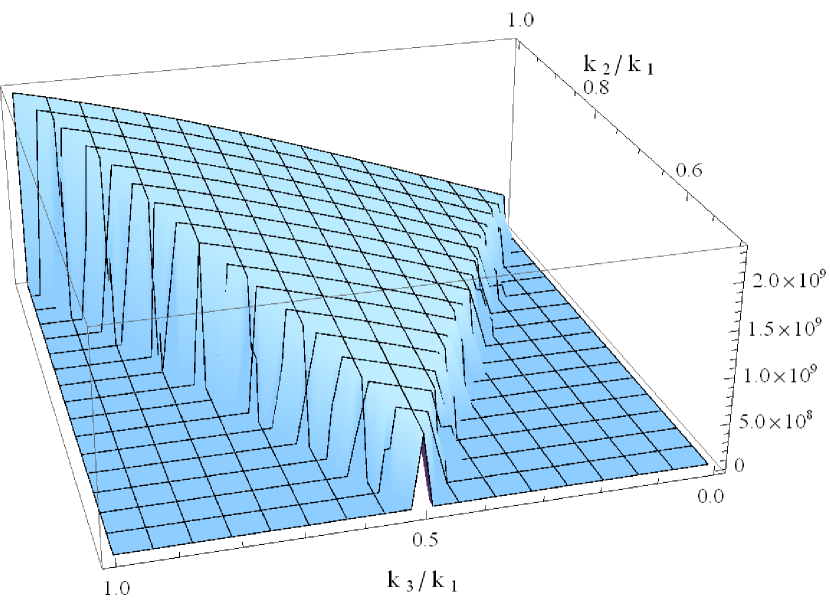
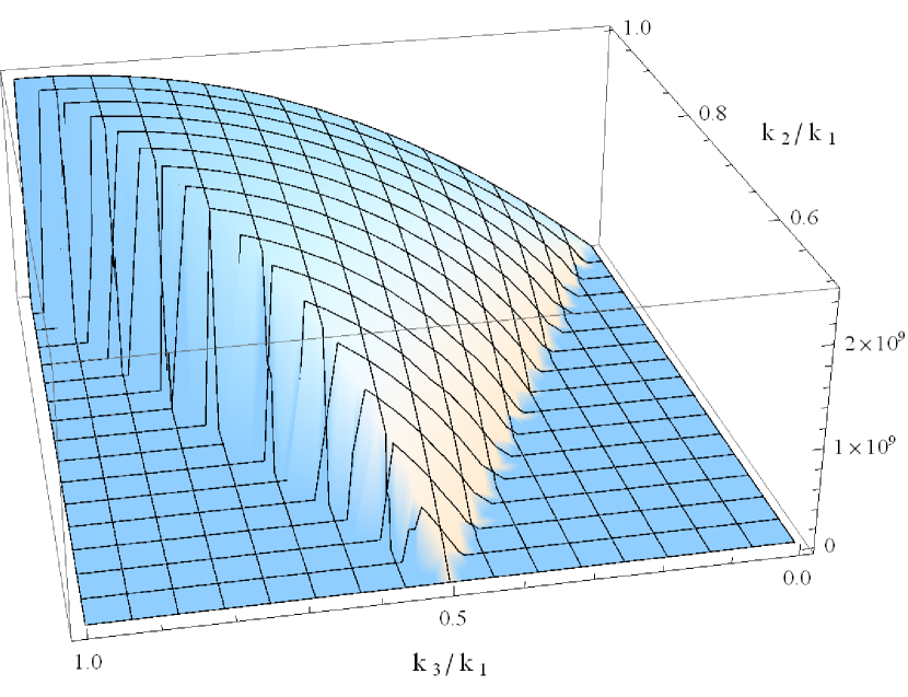
Figure 2: The shapes of $B_{\rm grav}$ (left panel) and $B_{\rm bis}^{\rm equil}$ (right panel) as functions of $k_{2}/k_{1}$ and $k_{3}/k_{1}$ in momentum space for $k_{1}=0.003h{\rm Mpc}^{-1}$ . We adopt $f_{\rm NL}^{\rm equil}=80$.

From Fig. 2, we can see that both $B_{\rm grav}$ and $B_{\rm bis}^{\rm equil}$ take the maximum values at the equilateral configuration ($k_{1}=k_{2}=k_{3}$). Therefore, in order to clarify the scale-dependence of their contributions, we concentrate on the equilateral configuration given by $k\equiv k_{1}=k_{2}=k_{3}$.

Then, from Eq. (16) and making use of the fact that the multi-point propagators have no scale-dependence on large scales after fixing the configuration, the scale-dependence of $B_{\rm grav}^{\rm tree}$ is estimated as

$$B_{\rm grav} \propto \mathcal{M}(k)^{4}P_{\Phi}^{2}\propto k^{2}\,,$$ (35)

while from Eq. (17) and the similar procedure, the scale-dependence of $B_{\rm bis}^{\rm equil}$ is estimated as

$$B_{\rm bis}^{\rm equil} \propto \mathcal{M}(k)^{3}P_{\Phi}^{2}\propto k^{0}\,.$$ (36)

From Eqs. (35) and (36), we can see that $B_{\rm bis}^{\rm equil}$ keeps to be constant while $B_{\rm grav}$ decreases as $k$ decreases and we can expect that $B_{\rm bis}^{\rm equil}$ will dominate $B_{\rm grav}$ above some scale. For the quantitative analysis, we plot the contributions $B_{\rm grav}$ and $B_{\rm bis}^{\rm equil}$ which we obtain numerically as functions of the wavenumber $k$ in Fig. 3. We can see that for $f_{\rm NL}^{\rm equil}=80$, $B_{\rm bis}^{\rm equil}$ dominates $B_{\rm grav}$ at $k\lesssim 0.003h{\rm Mpc}^{-1}$.

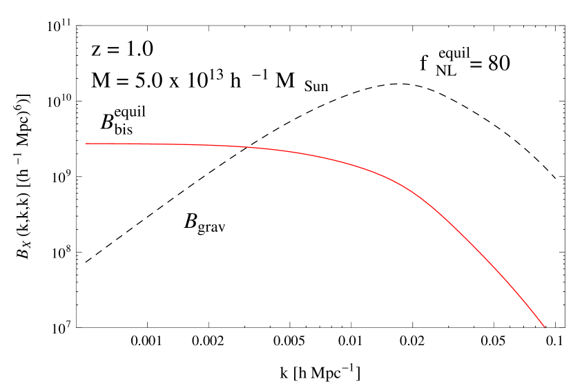
Figure 3: $B_{\rm grav}$ (black dashed line) and $B_{\rm bis}^{\rm equil}$ (red thick line) as a function of $k$. We take the equilateral configuration characterized by $k=k_{1}=k_{2}=k_{3}$ and adopt $f_{\rm NL}^{\rm equil}=80$.

IV Halo/Glaxy bispectrum with equilateral-type primordial trispectra

In the previous section, we confirm the fact that we could see the effect of the equilateral-type primordial bispectrum through the halo/galaxy bispectrum if $f_{\rm NL}^{\rm equil}$ takes the value of the current $2\sigma$ upper bound.

Then, let us focus on the halo/galaxy bispectrum with equilateral-type primordial trispectrum, which appears at the one-loop order in iPT. Generally, inflation models that produce equilateral-type primordial bispectrum also produce primordial $trispectrum$. After imposing scale-invariance, the trispectrum is described by a scalar function of five scalar variables, while the bispectrum is by two scalar variables. Therefore, although the current constraints are still very limited, the information of the primordial trispectra is helpful to constrain such inflation models. In this section, we investigate whether we could see the effect of the equilateral-type primordial $trispectra$ through the halo/galaxy bispectrum.

Among the primordial trispectra which can be generated by models producing the equilateral-type bispectrum, we concentrate on the following three types of trispectra:

$$T_{\Phi}^{\dot{\sigma}^{4}}({\bf k}_{1},{\bf k}_{2},{\bf k}_{3},{\bf k}_{4}) = \frac{221184}{25}\;g_{\rm NL}^{\dot{\sigma}^{4}}\;A_{\Phi}^{3}\;S^{\dot{\sigma}^{4}}({\bf k}_{1},{\bf k}_{2},{\bf k}_{3},{\bf k}_{4})\,,$$ (37)

$$T_{\Phi}^{\dot{\sigma}^{2}(\partial\sigma)^{2}}({\bf k}_{1},{\bf k}_{2},{\bf k}_{3},{\bf k}_{4}) = -\frac{27648}{325}\;g_{\rm NL}^{\dot{\sigma}^{2}(\partial\sigma)^{2}}\;A_{\Phi}^{3}\;S^{\dot{\sigma}^{2}(\partial\sigma)^{2}}({\bf k}_{1},{\bf k}_{2},{\bf k}_{3},{\bf k}_{4})\,,$$ (38)

$$T_{\Phi}^{(\partial\sigma)^{4}}({\bf k}_{1},{\bf k}_{2},{\bf k}_{3},{\bf k}_{4}) = \frac{16588}{2575}\;g_{\rm NL}^{(\partial\sigma)^{4}}\;A_{\Phi}^{3}\;S^{(\partial\sigma)^{4}}({\bf k}_{1},{\bf k}_{2},{\bf k}_{3},{\bf k}_{4})\,,$$ (39)

with

$$S^{\dot{\sigma}^{4}}({\bf k}_{1},{\bf k}_{2},{\bf k}_{3},{\bf k}_{4}) = \frac{1}{\left(\sum_{i=1}^{4}k_{i}\right)^{5}\Pi_{i=1}^{4}k_{i}}\,,$$ (40)

$$S^{\dot{\sigma}^{2}(\partial\sigma)^{2}}({\bf k}_{1},{\bf k}_{2},{\bf k}_{3},{\bf k}_{4}) = \frac{k_{1}^{2}k_{2}^{2}({\bf k}_{3}\cdot{\bf k}_{4})}{\left(\sum_{i=1}^{4}k_{i}\right)^{3}\Pi_{i=1}^{4}k_{i}^{3}}\left(1+3\frac{k_{3}+k_{4}}{\sum_{i=1}^{4}k_{i}}+12\frac{k_{3}k_{4}}{\left(\sum_{i=1}^{4}k_{i}\right)^{2}}\right)+5\;\;{\rm perms.}\,,$$ (41)

$$S^{(\partial\sigma)^{4}}({\bf k}_{1},{\bf k}_{2},{\bf k}_{3},{\bf k}_{4}) = \frac{({\bf k}_{1}\cdot{\bf k}_{2})({\bf k}_{3}\cdot{\bf k}_{4})+({\bf k}_{1}\cdot{\bf k}_{3})({\bf k}_{2}\cdot{\bf k}_{4})+({\bf k}_{1}\cdot{\bf k}_{4})({\bf k}_{2}\cdot{\bf k}_{3})}{\sum_{i=1}^{4}k_{i}\Pi_{i=1}^{4}k_{i}^{3}}$$ (42)

$$\times\left(1+\frac{\sum_{i<j}k_{i}k_{j}}{\left(\sum_{i=1}^{4}k_{i}\right)^{2}}+3\frac{\Pi_{i=1}^{4}k_{i}}{\left(\sum_{i=1}^{4}k_{i}\right)^{3}}\sum_{i=1}^{4}\frac{1}{k_{i}}+12\frac{\Pi_{i=1}^{4}k_{i}}{\left(\sum_{i=1}^{4}k_{i}\right)^{4}}\right)\,.$$

Here, $g_{\rm NL}^{\dot{\sigma}^{4}}$, $g_{\rm NL}^{\dot{\sigma}^{2}(\partial\sigma)^{2}}$ and $g_{\rm NL}^{(\partial\sigma)^{4}}$ are non-linearity parameters which characterize the amplitude of each trispectrum, $A_{\Phi}$ is the amplitude of the primordial power spectrum, defined by $A_{\Phi}=k^{3}P_{\Phi}$. In Eqs. (37), (38) and (39), the normalization have been chosen so that they give $(216/25)g_{\rm NL}A_{\Phi}^{3}/k^{9}$ for tetrahedral 4-point configurations with $|{\bf k}_{i}|=k$ and ${\bf k}_{i}\cdot{\bf k}_{j}=-k^{2}/3$ for $i\neq j$. This convention fixes all trispectra to have the same values on the tetrahedron as the local trispectrum.

Before starting the analysis, we briefly explain the physical motivation for concentrating on the above three trispectra. First, it was shown that these trispectra are generated by general $k$-inflation models through the contact interaction which is characterized by a quartic vertex Huang:2006eha . But it turned out that these trispectra are just a part of the full trispectra for this type of inflation models and they were completed to add another type of trispectra generated through the scalar-exchange interaction which is characterized by two cubic vertices Arroja:2009pd ; Chen:2009bc . From this result, it was pointed out that the amplitude of $T_{\Phi}^{\dot{\sigma}^{4}}$ can be large even when the equilateral-primordial bispectrum is small by tuning the model parameters. This possibility was supplemented by the effective field theory of inflation Cheung:2007st to clarify the symmetry that keeps to give $T_{\Phi}^{\dot{\sigma}^{4}}$ while protects the generation of cubic terms which are related with the other trispectra. In this respect, the trispectrum $T_{\Phi}^{\dot{\sigma}^{4}}$ was regarded as more important than the other trispectra generated by models producing the equilateral-type primordial bispectrum. Actually, the constraints on this trispectrum imposed by WMAP5 were reported in Fergusson:2010gn .

However, recently, a new possibility that the three trispectra $T_{\Phi}^{\dot{\sigma}^{4}}$, $T_{\Phi}^{\dot{\sigma}^{2}(\partial\sigma)^{2}}$ and $T_{\Phi}^{(\partial\sigma)^{4}}$ are equally important in the context of the effective field theory of $multi$-field inflation Smith:2015uia . In this set-up, since we can protect the cubic interactions, the other trispectra generated through the scalar-exchange interaction are suppressed. In the same paper, the authors also perform the optimal analysis of the CMB trispectrum and impose the constraints on the non-linearity parameters for these three trispectra making use of the fact that the shapes of these trispectra can be written as factorizable forms, which enables us to reduce the computational cost. Following Smith:2015uia , we will concentrate on the case that these three trispectra are equally important, while the other trispectra related with the cubic terms are suppressed. Although our analysis from now on is completely phenomenological in the sense that we regard the non-linearity parameters $g_{\rm NL}$ to be free, for those who are interested in how these trispectra are obtained in concrete models, we show the trispectra generated by general $k$-inflation models through the contact interaction in Appendix A.

The effect of the primordial trispectrum on the halo/galaxy bispectrum is given by $B_{\rm tris}$ in Eq. (15). From Eq. (18), in the large-scale limit $B_{\rm tris}$ can be approximated as

$$B_{\rm tris} \simeq \frac{1}{2}\Gamma^{(1)}_{X}({\bf k}_{1})\Gamma^{(1)}_{X}({\bf k}_{2})\int\frac{d^{3}p}{(2\pi)^{3}}\Gamma^{(2)}_{X}({\bf p},-{\bf p})T_{\rm L}({\bf k}_{1},{\bf k}_{2},{\bf p},-{\bf p})+2\;{\rm perms.}$$ (43)

$$= \frac{1}{2}\Gamma^{(1)}_{X}({\bf k}_{1})\mathcal{M}(k_{1})\Gamma^{(1)}_{X}({\bf k}_{2})\mathcal{M}(k_{2})\int\frac{d^{3}p}{(2\pi)^{3}}\Gamma^{(2)}_{X}({\bf p},-{\bf p})\mathcal{M}(p)^{2}T_{\rm\Phi}({\bf k}_{1},{\bf k}_{2},{\bf p},-{\bf p})+2\;{\rm perms.}\,.$$

Then Substituting Eqs. (37), (38) and (39) into Eq. (43) gives

$$\frac{B_{\rm tris}^{\dot{\sigma}^{4}}}{A_{\Phi}^{3}} \simeq \frac{3456}{25}\;g_{\rm NL}^{\dot{\sigma}^{4}}\Gamma^{(1)}_{X}({\bf k}_{1})\Gamma^{(1)}_{X}({\bf k}_{2})\frac{\mathcal{M}(k_{1})}{k_{1}}\frac{\mathcal{M}(k_{2})}{k_{2}}\int\frac{d^{3}p}{(2\pi)^{3}}\Gamma^{(2)}_{X}({\bf p},-{\bf p})\frac{\mathcal{M}(p)^{2}}{p^{7}}+2\;{\rm perms.}\,,$$ (44)

$$\frac{B_{\rm tris}^{\dot{\sigma}^{2}(\partial\sigma)^{2}}}{A_{\Phi}^{3}} \simeq -\frac{1728}{325}g_{\rm NL}^{\dot{\sigma}^{2}(\partial\sigma)^{2}}\Gamma^{(1)}_{X}({\bf k}_{1})\Gamma^{(1)}_{X}({\bf k}_{2})\frac{\mathcal{M}(k_{1})}{k_{1}^{3}}\frac{\mathcal{M}(k_{2})}{k_{2}^{3}}({\bf k}_{1}\cdot{\bf k}_{2})\int\frac{d^{3}p}{(2\pi)^{3}}\Gamma^{(2)}_{X}({\bf p},-{\bf p})\frac{\mathcal{M}(p)^{2}}{p^{5}}+2\;{\rm perms.}\,,$$ (45)

$$\frac{B_{\rm tris}^{(\partial\sigma)^{4}}}{A_{\Phi}^{3}} \simeq -\frac{4147}{2060}g_{\rm NL}^{(\partial\sigma)^{4}}\Gamma^{(1)}_{X}({\bf k}_{1})\Gamma^{(1)}_{X}({\bf k}_{2})\frac{\mathcal{M}(k_{1})}{k_{1}^{3}}\frac{\mathcal{M}(k_{2})}{k_{2}^{3}}\int\frac{d^{3}p}{(2\pi)^{3}}\Gamma^{(2)}_{X}({\bf p},-{\bf p})\frac{\mathcal{M}(p)^{2}}{p^{5}}$$ (46)

$$\times\Biggl{[}({\bf k}_{1}\cdot{\bf k}_{2})+2\left(\frac{{\bf p}}{p}\cdot{\bf k}_{1}\right)\left(\frac{{\bf p}}{p}\cdot{\bf k}_{2}\right)\Biggr{]}+2\;{\rm perms.}$$

$$= -\frac{4147}{1236}g_{\rm NL}^{(\partial\sigma)^{4}}\Gamma^{(1)}_{X}({\bf k}_{1})\Gamma^{(1)}_{X}({\bf k}_{2})\frac{\mathcal{M}(k_{1})}{k_{1}^{3}}\frac{\mathcal{M}(k_{2})}{k_{2}^{3}}({\bf k}_{1}\cdot{\bf k}_{2})\int\frac{d^{3}p}{(2\pi)^{3}}\Gamma^{(2)}_{X}({\bf p},-{\bf p})\frac{\mathcal{M}(p)^{2}}{p^{5}}+2\;{\rm perms.}\,,$$

where in the last line of Eq. (46), we have used the relation about the angular part of the integration of $p$

$$\int d\Omega_{p}\left(\frac{{\bf p}}{p}\cdot{\bf k}_{1}\right)\left(\frac{{\bf p}}{p}\cdot{\bf k}_{2}\right)=\frac{4\pi}{3}({\bf k}_{1}\cdot{\bf k}_{2})=\frac{({\bf k}_{1}\cdot{\bf k}_{2})}{3}\int d\Omega_{p}\,.$$ (47)

From Eqs. (44), (45) and (46), we can easily see that although we have started with three equilateral-types of the primordial trispectra, in the large-scale limit, $B_{\rm tris}^{\dot{\sigma}^{2}(\partial\sigma)^{2}}$ and $B_{\rm tris}^{(\partial\sigma)^{4}}$ become degenerate and we get only two types of shapes in the halo/galaxy bispectrum. This is caused by the fact the primordial trispectrum $T_{\Phi}^{\dot{\sigma}^{2}(\partial\sigma)^{2}}$ is very strongly correlated with $T_{\Phi}^{(\partial\sigma)^{4}}$ and from this reason, only two of the three trispectra, $T_{\Phi}^{\dot{\sigma}^{4}}$ and $T_{\Phi}^{(\partial\sigma)^{4}}$ were used as the basis of the optimal analysis of the CMB trispectrum Ade:2015ava ; Smith:2015uia . From this reason, we will concentrate on the two equilateral-type primordial trispectra $T_{\Phi}^{\dot{\sigma}^{4}}$ and $T_{\Phi}^{(\partial\sigma)^{4}}$ where the constraints from CMB have been obtained. Notice that although we do not mention the effect of $T_{\Phi}^{\dot{\sigma}^{2}(\partial\sigma)^{2}}$ from now on, once we can constrain the effect of $T_{\Phi}^{(\partial\sigma)^{4}}$, it should be constrained by the similar degree.

Then, from Eqs. (44) and (46), and making use of the fact that neither $\Gamma^{(1)}_{X}({\bf k})$ on large scales nor the integral of $p$ in Eq. (29) has no scale-dependence, we can obtain the following scale-dependence of $B_{\rm tris}^{\dot{\sigma}^{4}}$ and $B_{\rm tris}^{(\partial\sigma)^{4}}$:

$$B_{\rm tris}^{\dot{\sigma}^{4}} \propto \frac{\mathcal{M}(k)^{2}}{k^{2}}\propto k^{2}\,,$$ (48)

$$B_{\rm tris}^{(\partial\sigma)^{4}} \propto \frac{\mathcal{M}(k)^{2}}{k^{4}}\propto k^{0}\,.$$ (49)

As shown in the previous section, $B_{\rm grav}$ has the scale-dependence which is proportional to $k^{2}$ in large scales. Comparing the above scale-dependent behaviors of $B_{\rm tris}^{\dot{\sigma}^{4}}$ and $B_{\rm tris}^{(\partial\sigma)^{4}}$ with that of $B_{\rm grav}$, we can expect that $B_{\rm tris}^{(\partial\sigma)^{4}}$ will dominate $B_{\rm grav}$ above some scale, while it is difficult to find $B_{\rm tris}^{\dot{\sigma}^{4}}$ which has the same scale-dependence as $B_{\rm grav}$. Thus, hereinafter we focus on the halo/galaxy bispectrum with the primordial trispectrum $B_{\rm tris}^{(\partial\sigma)^{4}}$.

In Fig. 4, we plot $B_{\rm tris}^{(\partial\sigma)^{4}}$ to show not only the $k$-dependence with $k=k_{1}=k_{2}=k_{3}$, but also the shape of each contribution in $k$-space. We fix $k_{1}=0.003h{\rm Mpc}^{-1}$ and take $g_{\rm NL}^{(\partial\sigma)^{4}}=2.0\times 10^{7}$ so that it gives almost the same amplitude as $B_{\rm bis}^{\rm equil}$ with $f_{\rm NL}^{\rm equil}=80$.

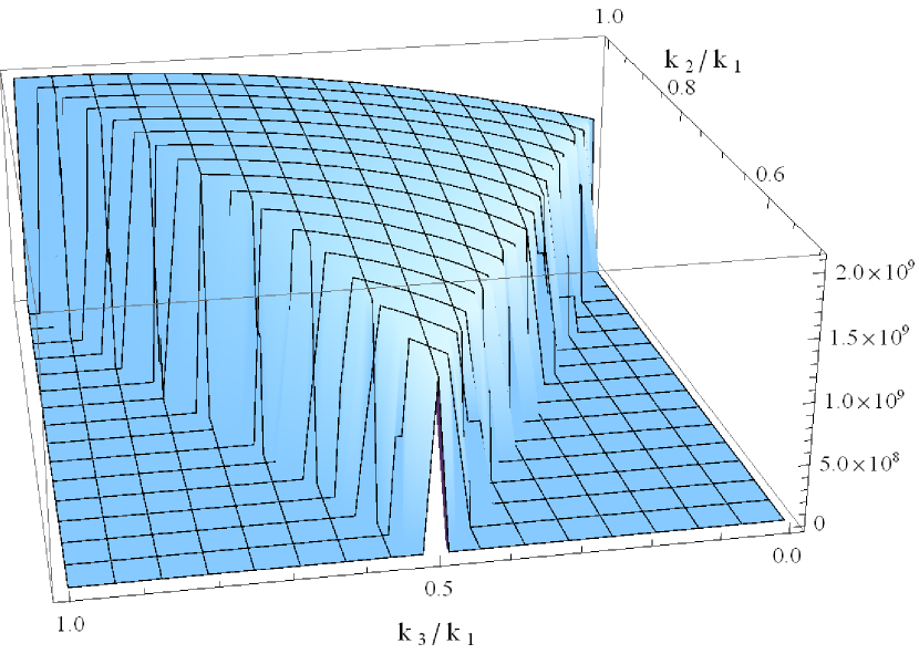
Figure 4: The shape of $B_{\rm tris}^{(\partial\sigma)^{4}}$ as a function of $k_{2}/k_{1}$ and $k_{3}/k_{1}$ in momentum space for $k_{1}=0.003h{\rm Mpc}^{-1}$ . We adopt $g_{\rm NL}^{(\partial\sigma)^{4}}=2.0\times 10^{7}$.

From Fig. 4, we can see that $B_{\rm tris}^{(\partial\sigma)^{4}}$ takes the maximum value at the equilateral configuration ($k_{1}=k_{2}=k_{3}$) as is the case in $B_{\rm grav}$ and $B_{\rm bis}^{\rm equil}$. Therefore, first we concentrate on the equilateral configuration given by $k\equiv k_{1}=k_{2}=k_{3}$. For the quantitative analysis, we plot the contributions $B_{\rm grav}$ and $B_{\rm tris}^{(\partial\sigma)^{4}}$ which we obtain numerically as functions of the wavenumber $k$ in Fig. 5. We can see that for $g_{\rm NL}^{(\partial\sigma)^{4}}=2.0\times 10^{7}$, $B_{\rm tris}^{(\partial\sigma)^{4}}$ dominates $B_{\rm grav}$ at $k\lesssim 0.003h{\rm Mpc}^{-1}$, and if we can observe such large scales, we can detect this, in principle.

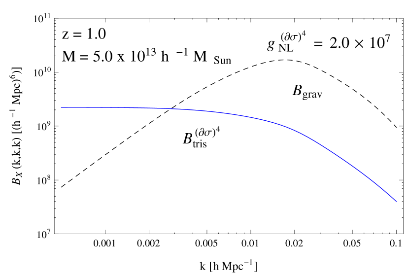
Figure 5: $B_{\rm grav}$ (black dashed line) and $B_{\rm tris}^{(\partial\sigma)^{4}}$ (blue thick line) as functions of $k$. We take the equilateral configuration characterized by $k=k_{1}=k_{2}=k_{3}$ and adopt $g_{\rm NL}^{(\partial\sigma)^{4}}=2.0\times 10^{7}$ .

In the above discussion, we confirm the fact that we could see the effect of one of the equilateral-type primordial trispectra, labelled as $T_{\Phi}^{(\partial\sigma)^{4}}$, through the halo/galaxy bispectrum on much larger scales if $g_{\rm NL}^{(\partial\sigma)^{4}}$ is about $O(10^{7})$. On the other hand, comparing Figs. 3 and 5, we see that both $B_{\rm bis}^{\rm equil}$ and $B_{\rm tris}^{(\partial\sigma)^{4}}$ have the same scale-dependence $\propto k^{0}$, which means that it is difficult to distinguish these two effects as long as we only consider the equilateral configuration.

However, as Figs. 2 and 4, the two shapes of $B_{\rm bis}^{\rm equil}$ and $B_{\rm tris}^{(\partial\sigma)^{4}}$ in Fourier space are different. Especially, the amplitude of $B_{\rm tris}^{(\partial\sigma)^{4}}$ does not decrease so much at $k_{1}=k_{2}=2k_{3}$, so-called folded configuration and this feature is very different from that of $B_{\rm bis}^{\rm equil}$. Hence, we expect that in principle by considering a different configuration it would be possible to distinguish the contributions from $B_{\rm bis}^{\rm equil}$ and $B_{\rm tris}^{(\partial\sigma)^{4}}$ in the halo/galaxy bispectrum. For this purpose, we introduce the isosceles configuration given by $k\equiv k_{1}=k_{2}=\alpha k_{3}$ and characterized by a parameter $\alpha$. The parameter $\alpha$ can take $\alpha\geq 1/2$ and $\alpha=1$ corresponds to the equilateral configuration.

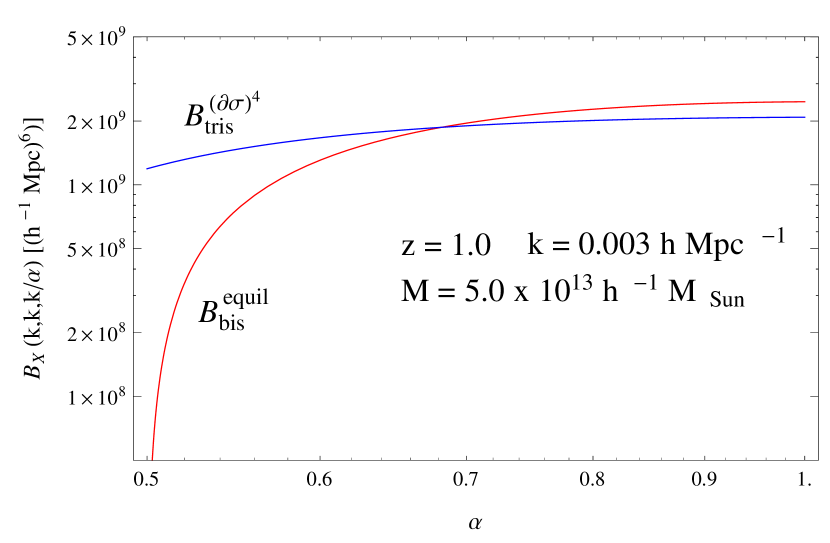
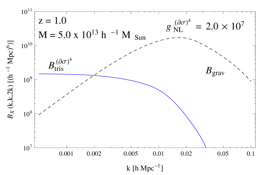
Figure 6: (Left panel) $B_{\rm bis}^{\rm equil}$ (red line) and $B_{\rm tris}^{(\partial\sigma)^{4}}$ (blue line) as functions of $\alpha$ which characterizes the isosceles configuration given by $k\equiv k_{1}=k_{2}=\alpha k_{3}$. We take $k=0.003h{\rm Mpc}^{-1}$ and adopt $f_{\rm NL}^{\rm equil}=80$ and $g_{\rm NL}^{(\partial\sigma)^{4}}=2.0\times 10^{7}$. (Right panel) $B_{\rm grav}$ (black dashed line) and $B_{\rm tris}^{(\partial\sigma)^{4}}$ (blue thick line) and as functions of $k$. We take the folded configuration characterized by $k=k_{1}=k_{2}=k_{3}/2$ and adopt $g_{\rm NL}^{(\partial\sigma)^{4}}=2.0\times 10^{7}$.

In the left panel of Fig. 6, we plot the contributions $B_{\rm bis}^{\rm equil}$ and $B_{\rm tris}^{(\partial\sigma)^{4}}$ as functions of the parameter $\alpha$. We can see that while $B_{\rm bis}^{\rm equil}$ is comparable to $B_{\rm tris}^{(\partial\sigma)^{4}}$ at the equilateral configuration ($\alpha=1$), it falls to zero very quickly at the folded configuration ($\alpha=1/2$). Therefore, even if there is primordial bispectrum whose effect gives the same scale-dependence of halo/galaxy bispectrum ($\propto k^{0}$) at the equilateral configuration, we can eliminate this effect by considering the folded configuration. Therefore, if $B_{\rm tris}^{(\partial\sigma)^{4}}$ can dominate $B_{\rm grav}$ on large scales also at the folded configuration, we can see the effect of this type of primordial trispectra. In the right panel of Fig. 6, we confirm that this actually happens as in the case of the equilateral configuration. Therefore, by considering both equilateral and folded configurations, we can see the effect of the primordial trispectrum $T_{\Phi}^{(\partial\sigma)^{4}}$ through the halo/galaxy bispectrum if its amplitude is sufficiently large.

V Summary and Discussions

The information contained in the primordial non-Gaussianity will contribute to a huge advance in our understanding of the physics of inflation. Although recent CMB observation by the Planck satellite has reported a very stringent constraints on the primordial non-Gaussianity Ade:2015ava , it would be very interesting to try further constraining the amplitude of non-Gaussianity based on the information other than CMB. For this purpose, recently, the fact that the large scale halo/galaxy distributions are affected by the primordial non-Gaussianity through the scale-dependent bias has been paid much attention. Although there have been many important works on investigating the effect of primordial non-Gaussianity on the scale-dependence of halo/galaxy distributions, the most works have been restricted to the primordial bispectrum and local-type trispectrum. This is because the shapes of the equilateral-type primordial trispectra strongly depend on theoretical models and also because their forms are generically much more complicated than those of the local-type trispectrum. Regardless of this, since this class of primordial trispectrum possess more information of the interaction structure of inflation, it would be worth trying to constrain this class of trispectrum, too. In this line, recently, based on the optimal analysis of the CMB, constraints on the amplitudes of the three equilateral-type trispectra $T_{\Phi}^{\dot{\sigma}^{4}}$, $T_{\Phi}^{\dot{\sigma}^{2}(\partial\sigma)^{2}}$ and $T_{\Phi}^{(\partial\sigma)^{4}}$ have been obtained in Ref. Smith:2015uia . These trispectra are considered not just because their forms are relatively simple, but have natural theoretical origin in the sense that they are shown to be appeared related with general $k$-inflation Huang:2006eha ; Arroja:2009pd ; Chen:2009bc and effective field theory of inflation Senatore:2010jy ; Senatore:2010wk .

In this paper, we have investigated the effect of these three important equilateral-type primordial trispectra on the scale-dependence of large scale halo/galaxy distributions. For this purpose, we have adopted the iPT formalism by which we can calculate the non-local biasing effect in the presence of any types of primordial non-Gaussianity systematically. Since it is not necessary for us to rely on the approximations like the peak background split and the peak formalism in iPT, the formulation for the large scale halo/galaxy distributions based on iPT can provide more general results than the formalisms mentioned above.

Before considering the effect of equilateral-type primordial trispectrum, we have demonstrated that it is necessary to consider the halo/galaxy bispectrum to see the scale-dependent behavior of halo/galaxy distributions sourced by the equilateral-type primordial bispectrum. This is completely different from the cases with the local-type primordial non-Gaussianity where there is an enhancement of the halo/galaxy power spectrum on large scales. We have shown that this difference comes from the fact that the shape of equilateral-type bispectrum has higher symmetry than the one of local-type bispectrum, which cancels the component enhanced on large scales in the halo/galaxy power spectrum. Since it is expected that a similar statement holds for the equilateral-type primordial trispectrum, we have investigated the effect of such trispectrum on the halo/galaxy bispectrum.

For the analysis of the scale-dependence of the halo/galaxy bispectrum in the presence of equilateral-type primordial trispectrum, although we had started with three primordial trispectra $T_{\Phi}^{\dot{\sigma}^{4}}$, $T_{\Phi}^{\dot{\sigma}^{2}(\partial\sigma)^{2}}$ and $T_{\Phi}^{(\partial\sigma)^{4}}$ , we have found that the large scale behaviors of $B_{\rm tris}^{\dot{\sigma}^{2}(\partial\sigma)^{2}}$ and $B_{\rm tris}^{(\partial\sigma)^{4}}$, the contributions sourced by $T_{\Phi}^{\dot{\sigma}^{2}(\partial\sigma)^{2}}$ and $T_{\Phi}^{(\partial\sigma)^{4}}$, respectively, become degenerate and we have got only two independent shapes. This is related with the fact that the primordial trispectrum $T_{\Phi}^{\dot{\sigma}^{2}(\partial\sigma)^{2}}$ is very strongly correlated with $T_{\Phi}^{(\partial\sigma)^{4}}$ and only two trispectra, $T_{\Phi}^{\dot{\sigma}^{4}}$ and $T_{\Phi}^{(\partial\sigma)^{4}}$ had been used as the basis of the optimal analysis of the CMB trispectrum Ade:2015ava ; Smith:2015uia . We have found that $B_{\rm tris}^{\dot{\sigma}^{2}(\partial\sigma)^{2}}$ and $B_{\rm tris}^{(\partial\sigma)^{4}}$ are enhanced on large scales and dominate $B_{\rm grav}$, the contribution induced by the nonlinearity of the gravitational evolution, on very large scales. On the other hand, we have shown that $B_{\rm tris}^{\dot{\sigma}^{4}}$, the contribution sourced by $T_{\Phi}^{\dot{\sigma}^{4}}$ has the same scale-dependence as $B_{\rm grav}$ and it cannot be expected that we can find $B_{\rm tris}^{\dot{\sigma}^{4}}$. Actually, for $g_{\rm NL}^{(\partial\sigma)^{4}}=2.0\times 10^{7}$ with which $B_{\rm tris}^{(\partial\sigma)^{4}}$ gives almost the same amplitude as $B_{\rm bis}^{\rm equil}$ with $f_{\rm NL}^{\rm equil}=80$, almost the 2-$\sigma$ upper bound obtained by Planck collaboration Ade:2015ava , $B_{\rm tris}^{(\partial\sigma)^{4}}$ would dominate the halo/galaxy bispectrum on large scales. Setting the typical redshift and the mass of the halos in surveys to be $z=1.0$ and $M=5\times 10^{13}h^{-1}M_{\odot}$, respectively, $B_{\rm tris}^{(\partial\sigma)^{4}}$ with $g_{\rm NL}^{(\partial\sigma)^{4}}=2.0\times 10^{7}$ will dominate $B_{\rm grav}$ at $k\lesssim 0.003h{\rm Mpc}^{-1}$. So far, we have estimated the scale-dependence of the halo/galaxy bispectrum with an equilateral configuration where the amplitudes of the contributions take the maximum values. But we have seen that $B_{\rm bis}^{\rm equil}$, $B_{\rm tirs}^{\dot{\sigma}^{2}(\partial\sigma)^{2}}$ and $B_{\rm tirs}^{(\partial\sigma)^{4}}$ provide the same scale-dependence on large scales. In order to pick up only the information of $T_{\Phi}^{(\partial\sigma)^{4}}$, we have shown that the folded configuration where $B_{\rm bis}^{\rm equil}$ falls to zero very quickly is helpful.

In summary, in this paper, it has been shown that we can constrain the non-linear parameters $g_{\rm NL}^{(\partial\sigma)^{4}}$ and $g_{\rm NL}^{\dot{\sigma}^{2}(\partial\sigma)^{2}}$ by the future LSS observations independently from those from CMB and we can use this at least as cross check of the CMB results. Next natural question is whether the constraints based on the future LSS observations can be more stringent than the ones from CMB. Actually, according to Smith:2015uia , the 2-$\sigma$ upper bound obtained by WMAP9 data is $0.19\times 10^{6}$. Given the fact that it is expected that the future LSS observations can constrain $f_{\rm NL}^{\rm equil}\sim\mathcal{O}(10)$ Sefusatti:2007ih , and a simple extrapolation provides $g_{\rm NL}^{(\partial\sigma)^{4}}$, $g_{\rm NL}^{\dot{\sigma}^{2}(\partial\sigma)^{2}}$ $\sim\mathcal{O}(10^{6})$, which is almost the same order as the ones obtained by current CMB observations. However, as we have shown that $B_{\rm tris}^{(\partial\sigma)^{4}}$ and $B_{\rm tris}^{\dot{\sigma}^{2}(\partial\sigma)^{2}}$ have signal for wider regions in $k$-space than $B_{\rm bis}^{\rm equil}$, which may provide more stringent constraints on $g_{\rm NL}^{(\partial\sigma)^{4}}$, $g_{\rm NL}^{\dot{\sigma}^{2}(\partial\sigma)^{2}}$. We leave the discussion on the detailed analysis to estimate the forecast on $g_{\rm NL}^{(\partial\sigma)^{4}}$, $g_{\rm NL}^{\dot{\sigma}^{2}(\partial\sigma)^{2}}$ to future work.

Finally, as is mentioned above, we have concentrated on three equilateral-type primordial trispectra whose amplitudes are constrained by CMB observations and theoretical origin is very clear. But there are still many interesting primordial trispectra generated by theoretical models which produce the equilateral-type bispectrum Gao:2009gd ; Mizuno:2009cv ; Mizuno:2009mv ; Chen:2009zp ; Huang:2010ab ; Izumi:2010wm ; Bartolo:2010di ; Izumi:2010yn ; Gao:2010xk ; Creminelli:2010qf ; Renaux-Petel:2013wya ; Renaux-Petel:2013ppa ; Fasiello:2013dla ; Bartolo:2013eka ; Arroja:2013dya . Although constraints are not obtained for these trispectra even by CMB observations, it might be interesting to consider the possibility to constrain these primordial trispectra based on the large scale halo/galaxy distributions.

Appendix A Equilateral-type primordial trispectrum in general single-field $k$-inflation models

Here, we briefly summarize the primordial trispectra generated by the general single-field $k$-inflation models Arroja:2009pd (see also Chen:2009bc ). The action of $k$-inflation is given by

$$S=\frac{1}{2}\int d^{4}x\sqrt{-g}\left[R+2P(X,\phi)\right]\,.$$ (50)

where $R$ is the Ricci scalar, $\phi$ is the inflaton field, $X\equiv-(1/2)g^{\mu\nu}\partial_{\mu}\phi\partial_{\nu}\phi$ is its kinetic term.

We calculate the primordial trispectrum making use of the so-called “interaction picture formalism” Weinberg:2005vy . As we mentioned in Sec. IV, although there are two types of trispectra which are generated through the contact interaction characterized by a quartic vertex and the scalar-exchange interaction characterized by two cubic vertices, we concentrate on the former ones. For this class of models, the fourth-order interaction Hamiltonian of the field perturbation $\sigma\equiv\delta\phi$ in the flat gauge at leading order in the slow-roll expansion are given by

$$H_{I}^{(4)}(\eta)=\int d^{3}x\left[\beta_{1}{\sigma_{I}^{\prime}}^{4}+\beta_{2}{\sigma_{I}^{\prime}}^{2}(\partial\sigma_{I})^{2}+\beta_{3}(\partial\sigma_{I})^{4}\right]\,.$$ (51)

where the subscript $I$ denotes that the variable is evaluated in the interaction picture, the prime denotes derivative with respect to conformal time $\eta$ and coefficients $\beta_{1}$, $\beta_{2}$ and $\beta_{3}$ are given by

$$\beta_{1} = P_{,XX}\left(1-\frac{9}{8}c_{s}^{2}\right)-2XP_{,XXX}\left(1-\frac{3}{4}c_{s}^{2}\right)+\frac{X^{3}c_{s}^{2}}{P_{,X}}P^{2}_{,XXX}-\frac{1}{6}X^{2}P_{,4X}\,,$$ (52)

$$\beta_{2} = -\frac{1}{2}P_{,XX}\left(1-\frac{3}{2}c_{s}^{2}\right)+\frac{1}{2}Xc_{s}^{2}P_{,XXX}\,,$$ (53)

$$\beta_{3} = -\frac{c_{s}^{2}}{8}P_{,XX}\,,$$ (54)

where $c_{s}$ is the sound speed given by

$$c_{s}^{2}=\frac{P_{,X}}{P_{,X}+2XP_{,XX}}\,.$$ (55)

Based on this interaction Hamiltonian, we can calculate the primordial trispectrum of the inflaton field perturbation at horizon crossing as

$$\langle\Omega|\sigma(0,{\bf k}_{1})\sigma(0,{\bf k}_{2})\sigma(0,{\bf k}_{3})\sigma(0,{\bf k}_{4})|\Omega\rangle=-i\int_{-\infty}^{0}d\eta\langle 0|\left[\sigma_{I}(0,{\bf k}_{1})\sigma_{I}(0,{\bf k}_{2})\sigma_{I}(0,{\bf k}_{3})\sigma_{I}(0,{\bf k}_{4}),H_{I}^{(4)}(\eta)\right]|0\rangle\,,$$ (56)

where $|\Omega\rangle$ denotes the vacuum in the interaction picture.

At leading order in slow-roll and in the small sound speed limit, in order to obtain the primordial trispectrum of the curvature perturbation at some time after horizon crossing, we can use the linear relation $\Phi=(H/\dot{\phi})\delta\phi$ because the higher order terms in this relation only generate sub-leading corrections to this result. Then, we can obtain the following equilateral-type primordial trispectra:

$$\langle\Omega|\Phi(0,{\bf k}_{1})\Phi(0,{\bf k}_{2})\Phi(0,{\bf k}_{3})\Phi(0,{\bf k}_{4})|\Omega\rangle$$

$$=-(2\pi)^{3}\delta^{(3)}({\bf k}_{1}+{\bf k}_{2}+{\bf k}_{3}+{\bf k}_{4})A_{\Phi}^{3}\frac{X}{c_{s}P_{,X}}\left(1152\beta_{1}c_{s}^{3}S^{\dot{\sigma}^{4}}+\beta_{2}c_{s}S^{\dot{\sigma}^{2}(\partial\sigma)^{2}}+32\beta_{3}c_{s}^{-1}S^{(\partial\sigma)^{4}}\right)\,,$$ (57)

where $A_{\Phi}\equiv k^{3}P_{\Phi}(k)=H^{4}/(4Xc_{s}P_{,X})$ is the amplitude of the primordial power spectrum and $S^{\dot{\sigma}^{4}}$, $S^{\dot{\sigma}^{2}(\partial\sigma)^{2}}$ and $S^{(\partial\sigma)^{4}}$ are shape functions given by Eqs. (40), (41) and (42), respectively.

By comparing Eq. (57) with Eqs. (37), (38), and (39), we can express the non-linear parameters $g_{\rm NL}^{\dot{\sigma}^{4}}$, $g_{\rm NL}^{\dot{\sigma}^{2}(\partial\sigma)^{2}}$ and $g_{\rm NL}^{(\partial\sigma)^{4}}$ in terms of the derivatives of $P$ with respect to $X$. However, since we have considered general $k$-inflation model so far and kept $P$ to be an arbitrary function of $\phi$ and $X$, it is not easy to see which trispectrum can give the dominant contribution among the three in Eq. (57). In order to see this, we consider the DBI inflation as a concrete example Silverstein:2003hf where the functional form of $P(\phi,X)$ is given by

$$P(X,\phi)=-f(\phi)^{-1}\sqrt{1-2f(\phi)X}-V(\phi)\,,$$ (58)

where $f(\phi)$ and $V(\phi)$ are functions of $\phi$ determined by string theory configurations, the derivatives of $P$ is related with $c_{s}$ like $c_{s}=P_{,X}^{-1}$. Then, at leading order in the sound speed, $\beta_{1}$, $\beta_{2}$ and $\beta_{3}$ are simplified as

$$\beta_{1}=\frac{1}{4c_{s}^{7}X}\,,\,\;\;\;\;\beta_{2}=\frac{1}{8c_{s}^{3}X}\,,\,\;\;\;\;\beta_{3}=-\frac{1}{16c_{s}X}\,.$$ (59)

Therefore, from Eqs. (57) and (59), we can see $T^{\dot{\sigma}^{4}}_{\Phi}$ gives the dominant contribution and the other two terms $T^{\dot{\sigma}^{2}(\partial\sigma)^{2}}_{\Phi}$ and $T^{(\partial\sigma)^{4}}_{\Phi}$ are subdominant unless $1/c_{s}^{2}\sim 1$, in which case the trispectrum is only marginally large $\sim\mathcal{O}(1)$. Although we do not show explicitly, similar things happens and the contributions from $T^{\dot{\sigma}^{2}(\partial\sigma)^{2}}_{\Phi}$ and $T^{(\partial\sigma)^{4}}_{\Phi}$ cannot be dominant whenever we can expect large non-Gaussian signal Chen:2009bc in general single-field $k$-inflation. However, as we explain in Sec. IV, the result based on the effective theory of multifield inflation Senatore:2010wk suggests that we can realize the situation where the three trispectra $T^{\dot{\sigma}^{4}}_{\Phi}$, $T^{\dot{\sigma}^{2}(\partial\sigma)^{2}}_{\Phi}$ and $T^{(\partial\sigma)^{4}}_{\Phi}$ give comparable contributions if we consider multi-field extension of the $k$-inflation models.

References

- (1) N. Bartolo, E. Komatsu, S. Matarrese and A. Riotto, Phys. Rept. 402 (2004) 103 [astro-ph/0406398].
- (2) P. A. R. Ade et al. [Planck Collaboration], arXiv:1502.01592 [astro-ph.CO].
- (3) N. Dalal, O. Dore, D. Huterer and A. Shirokov, Phys. Rev. D 77 (2008) 123514 [arXiv:0710.4560 [astro-ph]].
- (4) A. Slosar, C. Hirata, U. Seljak, S. Ho and N. Padmanabhan, JCAP 0808 (2008) 031 [arXiv:0805.3580 [astro-ph]].
- (5) S. Matarrese and L. Verde, Astrophys. J. 677 (2008) L77 [arXiv:0801.4826 [astro-ph]].
- (6) T. Giannantonio, A. J. Ross, W. J. Percival, R. Crittenden, D. Bacher, M. Kilbinger, R. Nichol and J. Weller, Phys. Rev. D 89 (2014) 2, 023511 [arXiv:1303.1349 [astro-ph.CO]].
- (7) T. Abbott et al. [Dark Energy Survey Collaboration], astro-ph/0510346.
- (8) D. Schlegel et al. [BiggBoss Experiment Collaboration], arXiv:1106.1706[astro-ph.IM]
- (9) P. A. Abell et al. [LSST Science and LSST Porject Collaborations], arXiv:0912.0201[astro-ph.IM]
- (10) R. Laureijs et al. [EUCLID Collaborations], arXiv:1110.3193[astro-ph.CO]
- (11) R. Ellis et al. [PFS Team Collaboration], arXiv:1206.0737[astro-ph.CO]
- (12) D. Yamauchi, K. Takahashi and M. Oguri, Phys. Rev. D 90 (2014) 8, 083520 [arXiv:1407.5453 [astro-ph.CO]].
- (13) E. Sefusatti and E. Komatsu, Phys. Rev. D 76 (2007) 083004 [arXiv:0705.0343 [astro-ph]].
- (14) D. Jeong and E. Komatsu, Astrophys. J. 703 (2009) 1230 [arXiv:0904.0497 [astro-ph.CO]].
- (15) E. Sefusatti, Phys. Rev. D 80 (2009) 123002 [arXiv:0905.0717 [astro-ph.CO]].
- (16) T. Baldauf, U. Seljak and L. Senatore, JCAP 1104 (2011) 006 [arXiv:1011.1513 [astro-ph.CO]].
- (17) T. Nishimichi, A. Taruya, K. Koyama and C. Sabiu, JCAP 1007 (2010) 002 [arXiv:0911.4768 [astro-ph.CO]].
- (18) S. Yokoyama, T. Matsubara and A. Taruya, Phys. Rev. D 89, no. 4, 043524 (2014) [arXiv:1310.4925 [astro-ph.CO]].
- (19) G. Tasinato, M. Tellarini, A. J. Ross and D. Wands, JCAP 1403 (2014) 032 [arXiv:1310.7482 [astro-ph.CO]].
- (20) H. Gil-Marin, C. Wagner, J. Norena, L. Verde and W. Percival, JCAP 1412 (2014) 12, 029 [arXiv:1407.1836 [astro-ph.CO]].
- (21) M. Tellarini, A. J. Ross, G. Tasinato and D. Wands, arXiv:1504.00324 [astro-ph.CO].
- (22) K. M. Smith, L. Senatore and M. Zaldarriaga, arXiv:1502.00635 [astro-ph.CO].
- (23) D. M. Regan, E. P. S. Shellard and J. R. Fergusson, Phys. Rev. D 82, 023520 (2010) [arXiv:1004.2915 [astro-ph.CO]].
- (24) S. Mizuno and K. Koyama, JCAP 1010 (2010) 002 [arXiv:1007.1462 [hep-th]].
- (25) J. R. Fergusson, D. M. Regan and E. P. S. Shellard, arXiv:1012.6039 [astro-ph.CO].
- (26) K. Izumi, S. Mizuno and K. Koyama, Phys. Rev. D 85 (2012) 023521 [arXiv:1109.3746 [astro-ph.CO]].
- (27) D. Regan, M. Gosenca and D. Seery, JCAP 1501 (2015) 01, 013 [arXiv:1310.8617 [astro-ph.CO]].
- (28) X. Chen, M. x. Huang and G. Shiu, Phys. Rev. D 74 (2006) 121301 [hep-th/0610235].
- (29) F. Arroja, S. Mizuno, K. Koyama and T. Tanaka, Phys. Rev. D 80 (2009) 043527 [arXiv:0905.3641 [hep-th]].
- (30) X. Chen, B. Hu, M. x. Huang, G. Shiu and Y. Wang, JCAP 0908 (2009) 008 [arXiv:0905.3494 [astro-ph.CO]].
- (31) L. Senatore and M. Zaldarriaga, JCAP 1101 (2011) 003 [arXiv:1004.1201 [hep-th]].
- (32) L. Senatore and M. Zaldarriaga, JHEP 1204 (2012) 024 [arXiv:1009.2093 [hep-th]].
- (33) T. Matsubara, Phys. Rev. D 83 (2011) 083518 [arXiv:1102.4619 [astro-ph.CO]].
- (34) T. Matsubara, Phys. Rev. D 86 (2012) 063518 [arXiv:1206.0562 [astro-ph.CO]].
- (35) T. Matsubara, Phys. Rev. D 90 (2014) 043537 [arXiv:1304.4226 [astro-ph.CO]].
- (36) S. Yokoyama and T. Matsubara, Phys. Rev. D 87 (2013) 2, 023525 [arXiv:1210.2495 [astro-ph.CO]].
- (37) M. Sato and T. Matsubara, Phys. Rev. D 87 (2013) 12, 123523 [arXiv:1304.4228 [astro-ph.CO]].
- (38) P. A. R. Ade et al. [Planck Collaboration], arXiv:1502.01589 [astro-ph.CO].
- (39) S. Chongchitnan and J. Silk, Astrophys. J. 724 (2010) 285 [arXiv:1007.1230 [astro-ph.CO]].
- (40) E. V. Linder, Phys. Rev. D 72 (2005) 043529 [astro-ph/0507263].
- (41) R. K. Sheth and G. Tormen, Mon. Not. Roy. Astron. Soc. 308 (1999) 119 [astro-ph/9901122].
- (42) E. Komatsu and D. N. Spergel, Phys. Rev. D 63 (2001) 063002 [astro-ph/0005036].
- (43) P. Creminelli, A. Nicolis, L. Senatore, M. Tegmark and M. Zaldarriaga, JCAP 0605 (2006) 004 [astro-ph/0509029].
- (44) C. Cheung, P. Creminelli, A. L. Fitzpatrick, J. Kaplan and L. Senatore, JHEP 0803 (2008) 014 [arXiv:0709.0293 [hep-th]].
- (45) X. Gao and B. Hu, JCAP 0908 (2009) 012 [arXiv:0903.1920 [astro-ph.CO]].
- (46) S. Mizuno, F. Arroja, K. Koyama and T. Tanaka, Phys. Rev. D 80 (2009) 023530 [arXiv:0905.4557 [hep-th]].
- (47) S. Mizuno, F. Arroja and K. Koyama, Phys. Rev. D 80 (2009) 083517 [arXiv:0907.2439 [hep-th]].
- (48) X. Chen and Y. Wang, JCAP 1004 (2010) 027 [arXiv:0911.3380 [hep-th]].
- (49) Q. G. Huang, JCAP 1007 (2010) 025 [arXiv:1004.0808 [astro-ph.CO]].
- (50) K. Izumi and S. Mukohyama, JCAP 1006 (2010) 016 [arXiv:1004.1776 [hep-th]].
- (51) N. Bartolo, M. Fasiello, S. Matarrese and A. Riotto, JCAP 1009 (2010) 035 [arXiv:1006.5411 [astro-ph.CO]].
- (52) K. Izumi, T. Kobayashi and S. Mukohyama, JCAP 1010 (2010) 031 [arXiv:1008.1406 [hep-th]].
- (53) X. Gao and C. Lin, JCAP 1011 (2010) 035 [arXiv:1009.1311 [hep-th]].
- (54) P. Creminelli, G. D’Amico, M. Musso, J. Norena and E. Trincherini, JCAP 1102 (2011) 006 [arXiv:1011.3004 [hep-th]].
- (55) S. Renaux-Petel, JCAP 1307 (2013) 005 [arXiv:1302.6978 [astro-ph.CO]].
- (56) S. Renaux-Petel, JCAP 1308 (2013) 017 [arXiv:1303.2618 [astro-ph.CO]].
- (57) M. Fasiello, JCAP 1312 (2013) 033 [arXiv:1303.5015 [hep-th]].
- (58) N. Bartolo, E. Dimastrogiovanni and M. Fasiello, JCAP 1309 (2013) 037 [arXiv:1305.0812 [astro-ph.CO]].
- (59) F. Arroja, N. Bartolo, E. Dimastrogiovanni and M. Fasiello, JCAP 1311 (2013) 005 [arXiv:1307.5371 [astro-ph.CO]].
- (60) S. Weinberg, Phys. Rev. D 72 (2005) 043514 [hep-th/0506236].
- (61) E. Silverstein and D. Tong, Phys. Rev. D 70 (2004) 103505 [hep-th/0310221].