A Modified KZ Reduction Algorithm

Abstract

The Korkine-Zolotareff (KZ) reduction has been used in communications and cryptography. In this paper, we modify a very recent KZ reduction algorithm proposed by Zhang et al., resulting in a new algorithm, which can be much faster and more numerically reliable, especially when the basis matrix is ill conditioned.

I Introduction

For any full column rank matrix $\boldsymbol{A}\in\mathbb{R}^{m\times n}$, the lattice $\mathcal{L}(\boldsymbol{A})$ generated by $\boldsymbol{A}$ is defined by

$$\mathcal{L}(\boldsymbol{A})=\{\boldsymbol{A}\boldsymbol{z}|\boldsymbol{z}\in\mathbb{Z}^{n}\}.$$ (1)

The columns of $\boldsymbol{A}$ form a basis of $\mathcal{L}(\boldsymbol{A})$. For any $n\geq 2$, $\mathcal{L}(\boldsymbol{A})$ has infinity many bases and any of two are connected by a unimodular matrix $\boldsymbol{Z}$, i.e., $\boldsymbol{Z}\in\mathbb{Z}^{n\times n}$ and $\det(\boldsymbol{Z})=\pm 1$. Specifically, for each given lattice basis matrix $\boldsymbol{A}\in\mathbb{R}^{m\times n}$, $\boldsymbol{A}\boldsymbol{Z}$ is also a basis matrix of $\mathcal{L}(\boldsymbol{A})$ if and only if $\boldsymbol{Z}$ is unimodular, see, e.g., [1].

The process of selecting a good basis for a given lattice, given some criterion, is called lattice reduction. In many applications, it is advantageous if the basis vectors are short and close to be orthogonal [1]. For more than a century, lattice reduction have been investigated by many people and several types of reductions have been proposed, including the KZ reduction [2], the Minkowski reduction [3], the LLL reduction [4] and Seysen’s reduction [5] etc.

Lattice reduction plays an important role in many research areas, such as, cryptography (see, e.g., [6]), communications (see, e.g., [1, 7]) and GPS (see, e.g., [8]), where the closest vector problem (CVP) and/or the shortest vector problem (SVP) need to be solved:

$$\min_{{\boldsymbol{x}}\in\mathbb{Z}^{n}}\|{\boldsymbol{y}}-\boldsymbol{A}{\boldsymbol{x}}\|_{2}^{2},$$ (2)

$$\min_{{\boldsymbol{x}}\in\mathbb{Z}^{n}\backslash\{{\boldsymbol{0}}\}}\|\boldsymbol{A}{\boldsymbol{x}}\|_{2}^{2}.$$ (3)

The often used lattice reduction is the LLL reduction, which can be computed in polynomial time under some conditions and has some nice properties, see, e.g., [9] for some latest results. In some communication applications, one needs to solve a sequence of CVPs, where ${\boldsymbol{y}}$’s are different, but $\boldsymbol{A}$’s are identical. In this case, instead of using the LLL reduction, one usually uses the KZ reduction [2] to do reduction, since sphere decoding for solving these CVPs becomes more efficient, although the KZ reduction costs more than the LLL reduction.

There are various KZ reduction algorithms, see, e.g., [10], [11], [12], [1]. Very recently, another KZ reduction algorithm was proposed in [13]. Like in [1], the LLL-aided Schnorr-Euchner search strategy [14] is used to solve the $n-1$ SVPs in [13]. But instead of using Kannan’s basis expansion method used in [11] and [1], it uses a new basis expansion method which is more efficient.

In this paper, we will propose a new KZ reduction algorithm, which improves the basis expansion method proposed in [13]. Like [13], we assume floating point arithmetic with fixed precision is used in the computation. Numerical results indicate that the modified algorithm can be much faster and more numerically reliable.

The rest of the paper is organized as follows. In section II, we introduce the LLL and KZ reductions. In section III, we introduce our modified KZ reduction algorithm. Some simulation results are given in section IV to show the efficiency and numerical reliability of our new algorithm. Finally, we summarize this paper in section V.

In this paper, boldface lowercase letters denote column vectors and boldface uppercase letters denote matrices. For a matrix $\boldsymbol{A}$, let $a_{ij}$ be its $(i,j)$ element and $\boldsymbol{A}_{i:j,k:\ell}$ be the submatrix containing elements with row indices from $i$ to $j$ and column indices from $k$ to $\ell$. Denote $\boldsymbol{e}_{1}=[1,0,\ldots,0]^{T}$, whose dimension depends on the context.

II LLL and KZ Reductions

Assume that $\boldsymbol{A}$ in (1) has the QR factorization

$$\boldsymbol{A}=[\boldsymbol{Q}_{1},\boldsymbol{Q}_{2}]\begin{bmatrix}\boldsymbol{R}\\ {\boldsymbol{0}}\end{bmatrix}$$ (4)

where $[\underset{n}{\boldsymbol{Q}_{1}},\underset{m-n}{\boldsymbol{Q}_{2}}]\in{\mathbb{R}}^{m\times m}$ is orthogonal and $\boldsymbol{R}\in{\mathbb{R}}^{n\times n}$ is upper triangular.

After the QR factorization of $\boldsymbol{A}$, the LLL reduction [4] reduces the matrix $\boldsymbol{R}$ in (4) to ${\bar{\boldsymbol{R}}}$ through the QRZ factorization:

$${\bar{\boldsymbol{Q}}}^{T}\boldsymbol{R}\boldsymbol{Z}={\bar{\boldsymbol{R}}},$$ (5)

where ${\bar{\boldsymbol{Q}}}\in\mathbb{R}^{n\times n}$ is orthogonal, $\boldsymbol{Z}\in\mathbb{Z}^{n\times n}$ is unimodular and ${\bar{\boldsymbol{R}}}\in\mathbb{R}^{n\times n}$ is upper triangular and satisfies the following conditions:

$$|{\bar{r}}_{ik}|\leq\frac{1}{2}|{\bar{r}}_{ii}|,\quad i=1,2,\ldots,k-1$$ (6)

$$\delta\,{\bar{r}}_{k-1,k-1}^{2}\leq{\bar{r}}_{k-1,k}^{2}+{\bar{r}}_{kk}^{2},\quad k=2,3,\ldots,n$$ (7)

where $\delta$ is a constant satisfying $1/4<\delta\leq 1$. The matrix $\boldsymbol{A}\boldsymbol{Z}$ is said to be LLL reduced. Equations (6) and (7) are referred to as the size-reduced condition and the Lovász condition, respectively.

Similarly, after the QR factorization of $\boldsymbol{A}$, the KZ reduction reduces the matrix $\boldsymbol{R}$ in (4) to ${\bar{\boldsymbol{R}}}$ in (5), where ${\bar{\boldsymbol{R}}}$ satisfies (6) and

$$|{\bar{r}}_{ii}|=\min_{{\boldsymbol{x}}\,\in\,\mathbb{Z}^{n-i+1}\backslash\{{\boldsymbol{0}}\}}\|{\bar{\boldsymbol{R}}}_{i:n,i:n}{\boldsymbol{x}}\|_{2},\ \ i=1,\ldots,n.$$ (8)

The matrix $\boldsymbol{A}\boldsymbol{Z}$ is said to be KZ reduced. Note that if a matrix is KZ reduced, it must be LLL reduced for $\delta=1$.

III A modified KZ reduction algorithm

In this section, we first introduce the KZ reduction algorithm given in [13], then propose a modified algorithm.

III-A The KZ Reduction Algorithm in [13]

From the definition of the KZ reduction, the reduced matrix ${\bar{\boldsymbol{R}}}$ satisfies both (6) and (8). If the QRZ factorization in (5) gives ${\bar{\boldsymbol{R}}}$ satisfying (8), then we can easily apply size reductions to ${\bar{\boldsymbol{R}}}$ such that (6) holds. Thus, in the following, we will only show how to obtain ${\bar{\boldsymbol{R}}}$ such that (8) holds.

The algorithm needs $n-1$ steps. Suppose that at the end of step $k-1$, one has found an orthogonal matrix $\boldsymbol{Q}^{(k-1)}\in{\mathbb{R}}^{n\times n}$, a unimodular matrix $\boldsymbol{Z}^{(k-1)}\in{\mathbb{Z}}^{n\times n}$ and an upper triangular $\boldsymbol{R}^{(k-1)}\in{\mathbb{R}}^{n\times n}$ such that

$$(\boldsymbol{Q}^{(k-1)})^{T}\boldsymbol{R}\boldsymbol{Z}^{(k-1)}=\boldsymbol{R}^{(k-1)}$$ (9)

where for $i=1,\ldots,k-1$,

$$|r^{(k-1)}_{ii}|=\min_{{\boldsymbol{x}}\,\in\,\mathbb{Z}^{n-i+1}\backslash\{{\boldsymbol{0}}\}}\|\boldsymbol{R}^{(k-1)}_{i:n,i:n}{\boldsymbol{x}}\|_{2}.\ \$$ (10)

At step $k$, like [1], [13] uses the LLL-aided Schnorr-Euchner search strategy [14] to solve the SVP:

$${\boldsymbol{x}}^{(k)}=\arg\min_{{\boldsymbol{x}}\,\in\mathbb{Z}^{n-k+1}\setminus\{{\boldsymbol{0}}\}}\|\boldsymbol{R}^{(k-1)}_{k:n,k:n}{\boldsymbol{x}}\|_{2}^{2}.$$ (11)

Then, unlike other KZ reduction algorithms, [13] finds the unimodular matrix by expanding $\boldsymbol{R}^{(k-1)}_{k:n,k:n}{\boldsymbol{x}}^{(k)}$ to a basis for the lattice $\{\boldsymbol{R}^{(k-1)}_{k:n,k:n}{\boldsymbol{x}}:{\boldsymbol{x}}\in\mathbb{Z}^{n-k+1}\}$. Specifically, [13] first constructs a unimodular matrix $\widetilde{\boldsymbol{Z}}^{(k)}\in{\mathbb{Z}}^{(n-k+1)\times(n-k+1)}$ whose first column is ${\boldsymbol{x}}^{(k)}$, i.e.,

$$\widetilde{\boldsymbol{Z}}^{(k)}\boldsymbol{e}_{1}={\boldsymbol{x}}^{(k)}$$ (12)

and then finds an orthogonal matrix $\widetilde{\boldsymbol{Q}}^{(k)}$ to bring $\boldsymbol{R}^{(k-1)}_{k:n,k:n}\widetilde{\boldsymbol{Z}}^{(k)}$ back to an upper triangular matrix $\widetilde{\boldsymbol{R}}^{(k)}$, i.e.,

$$(\widetilde{\boldsymbol{Q}}^{(k)})^{T}\boldsymbol{R}^{(k-1)}_{k:n,k:n}\widetilde{\boldsymbol{Z}}^{(k)}=\widetilde{\boldsymbol{R}}^{(k)}.$$ (13)

Based on (9) and (13), we define

$$\boldsymbol{Q}^{(k)} =\boldsymbol{Q}^{(k-1)}\left[\begin{smallmatrix}\boldsymbol{I}_{k-1}&{\boldsymbol{0}}\\ {\boldsymbol{0}}&\widetilde{\boldsymbol{Q}}^{(k)}\end{smallmatrix}\right],$$ (14)

$$\boldsymbol{R}^{(k)} =\left[\begin{smallmatrix}\boldsymbol{R}^{(k-1)}_{1:k-1,1:k-1}&\boldsymbol{R}^{(k-1)}_{1:k-1,k:n}\widetilde{\boldsymbol{Z}}^{(k)}\\ {\boldsymbol{0}}&\widetilde{\boldsymbol{R}}^{(k)}\end{smallmatrix}\right],$$ (15)

$$\boldsymbol{Z}^{(k)} =\boldsymbol{Z}^{(k-1)}\left[\begin{smallmatrix}\boldsymbol{I}_{k-1}&{\boldsymbol{0}}\\ {\boldsymbol{0}}&\widetilde{\boldsymbol{Z}}^{(k)}\end{smallmatrix}\right].$$ (16)

Here $\boldsymbol{Q}^{(k)}$ is orthogonal, $\boldsymbol{R}^{(k)}$ is upper triangular and $\boldsymbol{Z}^{(k)}$ is unimodular. Then, combining (9) and (13), we obtain

$$(\boldsymbol{Q}^{(k)})^{T}\boldsymbol{R}\boldsymbol{Z}^{(k)}=\boldsymbol{R}^{(k)}.$$ (17)

At the end of step $n-1$, we get $\boldsymbol{R}^{(n-1)}$, which is just ${\bar{\boldsymbol{R}}}$ in (5). In the following we explain why (8) holds.

From (15) and (13), it is easy to verify that for $i=1,\ldots,k$,

$$\boldsymbol{R}_{i:n,i:n}^{(k)}=\left[\begin{smallmatrix}\boldsymbol{I}_{k-i}&{\boldsymbol{0}}\\ {\boldsymbol{0}}&\widetilde{\boldsymbol{Q}}^{(k)}\end{smallmatrix}\right]^{T}\boldsymbol{R}_{i:n,i:n}^{(k-1)}\left[\begin{smallmatrix}\boldsymbol{I}_{k-i}&{\boldsymbol{0}}\\ {\boldsymbol{0}}&\widetilde{\boldsymbol{Z}}^{(k)}\end{smallmatrix}\right].$$ (18)

Then, from (18) and (10), for $i=1,\ldots,k-1$,

$$|r^{(k)}_{ii}| =|r^{(k-1)}_{ii}|=\min_{{\boldsymbol{x}}\,\in\,\mathbb{Z}^{n-i+1}\backslash\{{\boldsymbol{0}}\}}\|\boldsymbol{R}^{(k-1)}_{i:n,i:n}{\boldsymbol{x}}\|_{2}$$

$$=\min_{\boldsymbol{z}\,\in\,\mathbb{Z}^{n-i+1}\backslash\{{\boldsymbol{0}}\}}\|\boldsymbol{R}^{(k)}_{i:n,i:n}\boldsymbol{z}\|_{2}$$

where $\boldsymbol{z}=\left[\begin{smallmatrix}\boldsymbol{I}_{k-i}&{\boldsymbol{0}}\\ {\boldsymbol{0}}&\widetilde{\boldsymbol{Z}}^{(k)}\end{smallmatrix}\right]^{-1}{\boldsymbol{x}}$. From (15), (13), (12) and (11),

$$|r^{(k)}_{kk}| =\|\widetilde{\boldsymbol{R}}^{(k)}\boldsymbol{e}_{1}\|=\|(\widetilde{\boldsymbol{Q}}^{(k)})^{T}\boldsymbol{R}^{(k-1)}_{k:n,k:n}\widetilde{\boldsymbol{Z}}^{(k)}\boldsymbol{e}_{1}\|$$

$$=\|\boldsymbol{R}^{(k-1)}_{k:n,k:n}{\boldsymbol{x}}^{(k)}\|=\min_{{\boldsymbol{x}}\,\in\mathbb{Z}^{n-k+1}\setminus\{{\boldsymbol{0}}\}}\|\boldsymbol{R}^{(k-1)}_{k:n,k:n}{\boldsymbol{x}}\|_{2}$$

$$=\min_{{\boldsymbol{x}}\,\in\mathbb{Z}^{n-k+1}\setminus\{{\boldsymbol{0}}\}}\|\widetilde{\boldsymbol{R}}^{(k)}(\widetilde{\boldsymbol{Z}}^{(k)})^{-1}{\boldsymbol{x}}\|_{2}$$

$$=\min_{\boldsymbol{z}\,\in\mathbb{Z}^{n-k+1}\setminus\{{\boldsymbol{0}}\}}\|\boldsymbol{R}^{(k)}_{k:n,k:n}\boldsymbol{z}\|_{2}.$$ (19)

Thus (10) holds when $k-1$ changes to $k$. Then, with ${\bar{\boldsymbol{R}}}=\boldsymbol{R}^{(n-1)}$, we can conclude (8) holds.

In the following, we introduce the process of obtaining the unimodular matrix $\widetilde{\boldsymbol{Z}}^{(k)}$ in (12) proposed in [13]. (There are some other methods to find $\widetilde{\boldsymbol{Z}}^{(k)}$, see, e.g., [15, pp.13].) Suppose that $\boldsymbol{z}=[p,q]^{T}\in\mathbb{Z}^{2}$ and $\gcd(p,q)=d$, then, there exist two integers $a$ and $b$ such that $ap+bq=d$. Obviously,

$$\boldsymbol{U}=\begin{bmatrix}p/d&-b\\ q/d&a\end{bmatrix}$$ (20)

is unimodular and it is easy to verify that $\boldsymbol{U}^{-1}\boldsymbol{z}=d\,\boldsymbol{e}_{1}$.

From (11), we can conclude that

$$\gcd(x^{(k)}_{1},x^{(k)}_{2},\ldots,x^{(k)}_{k})=1.$$

After getting ${\boldsymbol{x}}^{(k)}$, $\widetilde{\boldsymbol{Z}}^{(k)}$ can be obtained by applying a sequence of 2 by 2 unimodular transformations of the form (20) to transform ${\boldsymbol{x}}^{(k)}$ to $\boldsymbol{e}_{1}$, i.e., $(\widetilde{\boldsymbol{Z}}^{(k)})^{-1}{\boldsymbol{x}}^{(k)}=\boldsymbol{e}_{1}$ (see (12)). Specifically they eliminate the entries of ${\boldsymbol{x}}^{(k)}$ from the last one to the second one. The resulting algorithm for finding $\widetilde{\boldsymbol{Z}}^{(k)}$ is described by Algorithm 1 and the corresponding KZ reduction algorithm is described by Algorithm 2.

Algorithm 1 The Basis Expansion Algorithm in [13]

1:  for $i=n-k,\dots,1$ do

2:     find $d=\gcd(x_{i},x_{i+1})$ and integers $a$ and $b$ such that $ax_{i}+bx_{i+1}=d$;

3:     set $\boldsymbol{U}=\begin{bmatrix}x_{i}/d&-b\\ x_{i+1}/d&a\\ \end{bmatrix}$;   $x_{i}=d$;

4:     $\boldsymbol{Z}_{1:n,i+k-1:i+k}=\boldsymbol{Z}_{1:n,i+k-1:i+k}\boldsymbol{U}$;

5:     $\boldsymbol{R}_{1:i+k,i+k-1:i+k}=\boldsymbol{R}_{1:i+k,i+k-1:i+k}\boldsymbol{U}$;

6:     find a 2 by 2 Givens rotation $\boldsymbol{G}$ such that:

$$\boldsymbol{G}\begin{bmatrix}r_{i+k-1,i+k-1}\\ r_{i+k,i+k-1}\\ \end{bmatrix}=\begin{bmatrix}\times\\ 0\\ \end{bmatrix};$$

7:     $\boldsymbol{R}_{i+k-1:i+k,i+k-1:n}=\boldsymbol{G}\boldsymbol{R}_{i+k-1:i-k,i+k-1:n}$;

8:  end for

Algorithm 2 The KZ Reduction Algorithm in [13]

1:  computer the QR factorization of $\boldsymbol{A}$, see (4);

2:  set $\boldsymbol{Z}=\boldsymbol{I}$;

3:  for $k=1$ to $n-1$ do

4:     solve $\min_{{\boldsymbol{x}}\,\in\mathbb{Z}^{n-k+1}\setminus\{{\boldsymbol{0}}\}}\|\boldsymbol{R}_{k:n,k:n}{\boldsymbol{x}}\|_{2}^{2}$ by the LLL-aided Schnorr-Euchner search strategy;

5:     apply Algorithm 1 to update $\boldsymbol{R}$ and $\boldsymbol{Z}$;

6:  end for

7:  perform size reductions on $\boldsymbol{R}$ and update $\boldsymbol{Z}$

Here we make a remark. Algorithm 2 does not show how to form and update $\boldsymbol{Q}$, as it may not be needed in applications. If an application indeed needs $\boldsymbol{Q}$, then we can obtain it by the QR factorization of $\boldsymbol{A}\boldsymbol{Z}$ after obtaining $\boldsymbol{Z}$. This would be more efficient.

III-B Proposed KZ Reduction Algorithm

In this subsection, we modify Algorithms 1 and 2 to get a new KZ reduction algorithm, which can be much faster and more numerically reliable.

First, we make an observation on Algorithm 2 and make a simple modification. At step $k$, if ${\boldsymbol{x}}^{(k)}=\pm\,\boldsymbol{e}_{1}$ (see (11)), then, obviously, the basis expansion algorithm, i.e., Algorithm 1 is not needed and we can move to step $k+1$. Later we will come back to this issue again.

In the following, we will make some major modifications. But before doing it, we introduce the following basic fact, which can be found in the literature: For any two integers $p$ and $q$, the time complexity of finding two integers $a$ and $b$ such that $ap+bq=d\equiv\gcd(p,q)$ by the extended Euclid algorithm is bounded by ${\mathcal{O}}(\log_{2}(\min\{|p|,|q|\}))$ if fixed precision is used.

In Algorithm 2, after finding ${\boldsymbol{x}}^{(k)}$ (see (11)), Algorithm 1 is used to expand $\boldsymbol{R}^{(k-1)}_{k:n,k:n}{\boldsymbol{x}}^{(k)}$ to a basis for the lattice $\{\boldsymbol{R}^{(k-1)}_{k:n,k:n}{\boldsymbol{x}}:{\boldsymbol{x}}\in\mathbb{Z}^{n-k+1}\}$. There are some serious drawbacks with this approach. Sometimes, especially when $\boldsymbol{A}$ is ill-conditioned, some of the entries of ${\boldsymbol{x}}^{(k)}$ may be very large such that they are beyond the range of consecutive integers in a floating point system (i.e., integer overflow occurs), very likely resulting in wrong results. Even if integer overflow does not occur in storing ${\boldsymbol{x}}^{(k)}$, large ${\boldsymbol{x}}^{(k)}$ may still cause problems. One problem is that the computational time of the extended Euclid algorithm will be long according to its complexity result we just mentioned before. The second problem is that updating $\boldsymbol{Z}$ and $\boldsymbol{R}$ in lines 4 and 5 of Algorithm 1 may cause numerical issues. Large $x_{i}$ and $x_{i+1}$ are likely to produce large elements in $\boldsymbol{U}$. As a result, integer overflow may occur in updating $\boldsymbol{Z}$, and large rounding errors are likely to occur in updating $\boldsymbol{R}$. Finally, $\boldsymbol{R}$ is likely to become more ill-conditioned after the updating, making the search process for solving SVPs in later steps expensive.

In order to deal with the large ${\boldsymbol{x}}^{(k)}$ issue, we look at line 4 in Algorithm 2, which uses the LLL-aided Schnorr-Euchner search strategy to solve the SVP. Specifically at step $k$, to solve (11), the LLL reduction algorithm is applied to $\boldsymbol{R}^{(k-1)}_{k:n,k:n}$:

$$(\widehat{\boldsymbol{Q}}^{(k)})^{T}\boldsymbol{R}^{(k-1)}_{k:n,k:n}\widehat{\boldsymbol{Z}}^{(k)}=\widehat{\boldsymbol{R}}^{(k-1)}$$ (21)

where $\widehat{\boldsymbol{Q}}^{(k)}\in\mathbb{R}^{(n-k+1)\times(n-k+1)}$ is orthogonal, $\widehat{\boldsymbol{Z}}^{(k)}\in\mathbb{Z}^{(n-k+1)\times(n-k+1)}$ is unimodular and $\widehat{\boldsymbol{R}}^{(k-1)}$ is LLL-reduced. Then, one solves the reduced SVP by the Schnorr-Euchner search strategy:

$$\boldsymbol{z}^{(k)}=\arg\min_{\boldsymbol{z}\,\in\mathbb{Z}^{n-k+1}\setminus\{{\boldsymbol{0}}\}}\|\widehat{\boldsymbol{R}}^{(k-1)}\boldsymbol{z}\|_{2}^{2}.$$ (22)

The solution of the original SVP is ${\boldsymbol{x}}^{(k)}=\widehat{\boldsymbol{Z}}^{(k)}\boldsymbol{z}^{(k)}$.

Instead of expanding $\boldsymbol{R}^{(k-1)}_{k:n,k:n}{\boldsymbol{x}}^{(k)}$ as done in Algorithm 2, we propose to expand $\widehat{\boldsymbol{R}}^{(k-1)}\boldsymbol{z}^{(k)}$ to a basis for the lattice $\{\widehat{\boldsymbol{R}}^{(k-1)}\boldsymbol{z}:\boldsymbol{z}\in\mathbb{Z}^{n-k+1}\}$. Thus, before doing the expansion, we update $\boldsymbol{Q}^{(k)},\boldsymbol{R}^{(k)}$ and $\boldsymbol{Z}^{(k)}$ by using the LLL reduction (21):

$$\check{\boldsymbol{Q}}^{(k)} =\boldsymbol{Q}^{(k-1)}\left[\begin{smallmatrix}\boldsymbol{I}_{k-1}&{\boldsymbol{0}}\\ {\boldsymbol{0}}&\widehat{\boldsymbol{Q}}^{(k)}\end{smallmatrix}\right],$$ (23)

$$\check{\boldsymbol{R}}^{(k)} =\left[\begin{smallmatrix}\boldsymbol{R}^{(k-1)}_{1:k-1,1:k-1}&\boldsymbol{R}^{(k-1)}_{1:k-1,k:n}\widehat{\boldsymbol{Z}}^{(k)}\\ {\boldsymbol{0}}&\widehat{\boldsymbol{R}}^{(k-1)}\end{smallmatrix}\right],$$ (24)

$$\check{\boldsymbol{Z}}^{(k)} =\boldsymbol{Z}^{(k-1)}\left[\begin{smallmatrix}\boldsymbol{I}_{k-1}&{\boldsymbol{0}}\\ {\boldsymbol{0}}&\widehat{\boldsymbol{Z}}^{(k)}\end{smallmatrix}\right].$$ (25)

Now we do expansion. We construct a unimodular matrix $\widetilde{\boldsymbol{Z}}^{(k)}\in{\mathbb{Z}}^{(n-k+1)\times(n-k+1)}$ whose first column is $\boldsymbol{z}^{(k)}$, and find an orthogonal matrix $\widetilde{\boldsymbol{Q}}^{(k)}$ to bring $\widehat{\boldsymbol{R}}^{(k-1)}\widetilde{\boldsymbol{Z}}^{(k)}$ back to an upper triangular matrix $\widetilde{\boldsymbol{R}}^{(k)}$ (cf. (13)):

$$(\widetilde{\boldsymbol{Q}}^{(k)})^{T}\widehat{\boldsymbol{R}}^{(k-1)}\widetilde{\boldsymbol{Z}}^{(k)}=\widetilde{\boldsymbol{R}}^{(k)}.$$ (26)

Then, we update $\check{\boldsymbol{Q}}^{(k)}$, $\check{\boldsymbol{R}}^{(k)}$ and $\check{\boldsymbol{Z}}^{(k)}$ as follows (cf. (14)–(16)):

$$\boldsymbol{Q}^{(k)} =\check{\boldsymbol{Q}}^{(k-1)}\left[\begin{smallmatrix}\boldsymbol{I}_{k-1}&{\boldsymbol{0}}\\ {\boldsymbol{0}}&\widetilde{\boldsymbol{Q}}^{(k)}\end{smallmatrix}\right],$$ (27)

$$\boldsymbol{R}^{(k)} =\left[\begin{smallmatrix}\check{\boldsymbol{R}}^{(k-1)}_{1:k-1,1:k-1}&\check{\boldsymbol{R}}^{(k-1)}_{1:k-1,k:n}\widetilde{\boldsymbol{Z}}^{(k)}\\ {\boldsymbol{0}}&\widetilde{\boldsymbol{R}}^{(k)}\end{smallmatrix}\right],$$ (28)

$$\boldsymbol{Z}^{(k)} =\check{\boldsymbol{Z}}^{(k-1)}\left[\begin{smallmatrix}\boldsymbol{I}_{k-1}&{\boldsymbol{0}}\\ {\boldsymbol{0}}&\widetilde{\boldsymbol{Z}}^{(k)}\end{smallmatrix}\right]$$ (29)

and we obtain the QRZ factorization of $\boldsymbol{R}$ in the same form as (17) at step $k$.

Unlike ${\boldsymbol{x}}^{(k)}$ in (11), which can be arbitrarily large, $\boldsymbol{z}^{(k)}$ in (22) can be bounded. Actually by using the LLL reduction properties and the fact that

$$\|\widehat{\boldsymbol{R}}^{(k-1)}\boldsymbol{z}^{(k)}\|_{2}\leq\|\widehat{\boldsymbol{R}}^{(k-1)}\boldsymbol{e}_{1}\|_{2}=|\widehat{r}_{11}^{(k-1)}|$$

we can show the following result:

Theorem 1

For $1\leq i\leq n-k+1$, the $i$-th entry of $\boldsymbol{z}^{(k)}\in\mathbb{Z}^{n-k+1}$ (see (22)) satisfies

$$|z^{(k)}_{i}|\leq\big{(}\frac{4}{4\delta-1}\big{)}^{(n-k)/2}2^{n-k+1-i}$$ (30)

where $\delta$ is the parameter in the LLL reduction (see (7)).

Because of the limitation of space, we omit its proof.

Now we discuss the benefits of the modification. First, since $\widehat{\boldsymbol{R}}^{(k-1)}$ is LLL reduced, it has a very good chance, especially when $\boldsymbol{R}$ is well-conditioned and $n$ is small (say, smaller than 30), that $\boldsymbol{z}^{(k)}=\pm\,\boldsymbol{e}_{1}$ (see (22)). This was observed in our simulations. As we stated before, the basis expansion is not needed in this case and we can move to next step. Second, the entries of $\boldsymbol{z}^{(k)}$ are bounded according to Theorem 1, but the entries of ${\boldsymbol{x}}^{(k)}$ are not. Our simulations indicated that the former are smaller or much smaller than the latter. Thus, the serious problems with using ${\boldsymbol{x}}^{(k)}$ for basis expansion mentioned before can be significantly mitigated by using $\boldsymbol{z}^{(k)}$ instead.

To further reduce the computational cost, we look at the basis expansion process at step $k$ of Algorithm 2. After $\boldsymbol{z}^{(k)}$ is obtained, Algorithm 1 is used to find a sequence of 2 by 2 unimodular matrices in the form of (20) to eliminate its entries form the last one to the second one. We noticed in our simulations that often $\boldsymbol{z}^{(k)}$ has a lot of zeros and we would like to explore this to make the basis expansion process more efficient. Specifically, if $\boldsymbol{z}=[p,q]^{T}\in\mathbb{Z}^{2}$ with $q=0$, then $\mbox{gcd}(p,q)=p$, and $\boldsymbol{U}=\boldsymbol{I}_{2}$ in (20). Thus, in this case we do not need to do anything and move to eliminate the next element in $\boldsymbol{z}^{(k)}$.

Now we can describe the modified KZ reduction algorithm in Algorithm 3.

Algorithm 3 Modified KZ Reduction Algorithm

1:  computer the QR factorization of $\boldsymbol{A}$, see (4);

2:  set $\boldsymbol{Z}=\boldsymbol{I},k=1$;

3:  while $k<n$ do

4:     compute the LLL reduction of $\boldsymbol{R}_{k:n,k:n}$ (see (21)) and update $\boldsymbol{R},\boldsymbol{Z}$ (see (24)-(25));

5:     solve $\min_{\boldsymbol{z}\,\in\mathbb{Z}^{n-k+1}\setminus\{{\boldsymbol{0}}\}}\|\boldsymbol{R}_{k:n,k:n}\boldsymbol{z}\|_{2}^{2}$ by the Schnorr-Euchner search strategy to get the solution $\boldsymbol{z}$;

6:     if $\boldsymbol{z}=\pm\,\boldsymbol{e}_{1}$ then

7:        $k=k+1$;

8:     else

9:        $i=n-k$;

10:        while $i\geq 1$ do

11:           if $z_{i+1}\neq 0$ then

12:              perform lines 2-7 of Algorithm 1 (where $x_{i}$ and $x_{i+1}$ are replaced by $z_{i}$ and $z_{i+1}$);

13:           end if

14:           $i=i-1$;

15:        end while

16:        $k=k+1$;

17:     end if

18:  end while

19:  perform size reductions on $\boldsymbol{R}$ and update $\boldsymbol{Z}$.

IV Numerical tests

In this section, we compare the performance of the proposed KZ algorithm Algorithm 3 with Algorithm 2. All the numerical tests were done by Matlab 14b on a desktop computer with Intel(R) Xeon(R) CPU W3530 @ 2.80GHz$\times 4$. The Matlab code for Algorithm 2 was provided by Dr. Wen Zhang, one of the authors of [13]. The parameter $\delta$ in the LLL reduction was chosen to be 1.

We first give an example to show that Algorithm 2 may not even give a LLL reduced matrix (for $\delta=1$), while Algorithm 3 does.

Example. Let

$$\boldsymbol{A}\!=\!\left[\begin{array}[]{@{}rrrrr@{}}10.6347&-66.2715&9.3046&17.5349&24.9625\\ 0&8.6759&-4.7536&-3.9379&-2.3318\\ 0&0&0.3876&0.1296&-0.2879\\ 0&0&0&0.0133&-0.0082\\ 0&0&0&0&0.0015\end{array}\right].$$

Applying Algorithm 2 gives

$$\boldsymbol{R}=\left[\begin{array}[]{@{}rrrrr@{}}-0.2256&-0.0792&0.0125&0&0\\ 0&0.2148&-0.0728&-0.0029&-0.0012\\ 0&0&0.2145&0.0527&-0.0211\\ 0&0&0&-0.1103&0.0306\\ 0&0&0&0&0.6221\end{array}\right].$$

It is easy to check that $\boldsymbol{R}$ is not LLL reduced (for $\delta=1$) since ${r}_{33}^{2}>{r}_{34}^{2}+{r}_{44}^{2}$. Moreover, the matrix $\boldsymbol{Z}$ obtained by Algorithm 2 is not unimodular since its determinant is $-3244032$, which was precisely calculated by Maple. The reason for this is that $\boldsymbol{A}$ is ill conditioned (its condition number in the 2-norm is about $1.0\times 10^{5}$) and some of the entries of ${\boldsymbol{x}}^{(k)}$ (see (11)) are too large, causing severe inaccuracy in updating $\boldsymbol{R}$ and integer overflow in updating $\boldsymbol{Z}$ (see lines 4-5 in Algorithm 1). In fact,

$${\boldsymbol{x}}^{(1)} =\begin{bmatrix}-47,&-27,&-21,&-14,&-34\end{bmatrix}^{T};$$

$${\boldsymbol{x}}^{(2)} =\begin{bmatrix}-48029,&-27593,&2145,&345\end{bmatrix}^{T};$$

$${\boldsymbol{x}}^{(3)} =\begin{bmatrix}-2767925153,&432235,&40\end{bmatrix}^{T};$$

$${\boldsymbol{x}}^{(4)} =\begin{bmatrix}691989751,&2\end{bmatrix}^{T}.$$

The condition numbers in the 2-norm of $\boldsymbol{R}(k\!:\!5,k\!:\!5)$ obtained at the end of step $k=1,2,3,4$ of Algorithm 2 are respectively $2.9\times 10^{8},1.5\times 10^{15},6.2\times 10^{18}$ and $1.1\times 10$. A question one may raise is that if $\boldsymbol{A}$ is updated by the unimodular matrices produced in the process (i.e., $\boldsymbol{Z}$ is not explicitly formed) is $\boldsymbol{A}\boldsymbol{Z}$ LLL reduced? We found it is still not by looking at the R-factor of the QR factorization of $\boldsymbol{A}\boldsymbol{Z}$.

Applying Algorithm 3 to $\boldsymbol{A}$ gives

$${\boldsymbol{R}}=\left[\begin{array}[]{@{}rrrrr@{}}-0.2256&0.0792&-0.0126&0.0028&-0.0621\\ 0&-0.2148&0.0728&-0.0084&0.0930\\ 0&0&0.2145&0.0292&-0.0029\\ 0&0&0&-0.2320&0.0731\\ 0&0&0&0&-0.2959\end{array}\right].$$

Although we cannot verify if $\boldsymbol{R}$ is KZ reduced, we can verify that indeed it is LLL reduced. All of the solutions of the four SVPs are $\boldsymbol{e}_{1}$ (note that the dimensions are different). Thus, no basis expansion is needed. The condition numbers in the 2-norm of $\boldsymbol{R}(k\!:\!5,k\!:\!5)$ obtained at the end of step $k=1,2,3,4$ of Algorithm 3 are respectively $2.1,1.9,1.6$ and $1.4$.

Now we consider two more general cases for comparing the efficiency of the two algorithms:

• Case 1. $\boldsymbol{A}=\text{randn}(n,n)$, where $\text{randn}(n,n)$ is a Matlab built-in function to generate a random $n\times n$ matrix, whose entries follow the normal distribution ${\cal N}(0,1)$.

• Case 2. $\boldsymbol{A}=\boldsymbol{U}\boldsymbol{D}\boldsymbol{V}^{T}$, $\boldsymbol{U},\boldsymbol{V}$ are random orthogonal matrices obtained by the QR factorization of random matrices generated by $\text{randn}(n,n)$ and $\boldsymbol{D}$ is a $n\times n$ diagonal matrix with $d_{ii}=10^{3(n/2-i)/(n-1)}$.

In the numerical tests for each case for a fixed $n$ we gave 200 runs to generate 200 different $\boldsymbol{A}$’s. Figures 1 and 2 display the average CPU time over 200 runs versus $n=2:2:20$ for Cases 1 and 2, respectively. In both figures, “KZ” and “Modified KZ” refer to Algorithms 2 and 3, respectively.

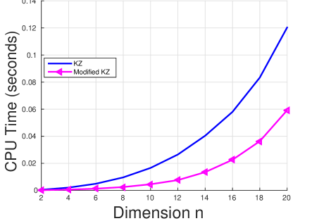
Figure 1: Average CPU time versus $\boldsymbol{n}$ for Case 1

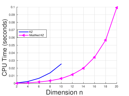
Figure 2: Average CPU time versus $\boldsymbol{n}$ for Case 2

Figure 2 gives the results for only $n=2:2:10$. This is because when $n\geq 12$, Algorithm 2 often did not terminate within ten hours.

In Case 1, sometimes Algorithm 2 did not terminate within a half hour and we just ignored this instance and gave one more run. The number of such instances was much smaller than that for Case 2.

From Figures 1 and 2, we can see that Algorithm 3 is faster than Algorithm 2 for Case 1 and much faster for Case 2. Also, when we ran Algorithm 2 we got a warning message ”Warning: Inputs contain values larger than the largest consecutive flint. Result may be inaccurate” several times, for both Cases 1 and 2 in the tests. But this did not happen to Algorithm 3. Thus Algorithm 3 is more numerically reliable.

V Summary and comment

In this paper, we modified the KZ reduction algorithm proposed by Zhang et al. in [13]. The resulting algorithm can be much faster and more numerically reliable.

The modified basis expansion strategy proposed in this paper can be applied in designing algorithms for the Minkowski reduction (see, e.g., [13]) and the block KZ reduction (see [12] and [16]).

References

• [1] E. Agrell, T. Eriksson, A. Vardy, and K. Zeger, “Closest point search in lattices,” IEEE Transactions on Information Theory, vol. 48, no. 8, pp. 2201–2214, 2002.
• [2] A. Korkine and G. Zolotareff, “Sur les formes quadratiques,” Mathematische Annalen, vol. 6, no. 3, pp. 366–389, 1873.
• [3] H. Minkowski, “Geometrie der zahlen (2 vol.),” Teubner, Leipzig, vol. 1910, 1896.
• [4] A. Lenstra, H. Lenstra, and L. Lovász, “Factoring polynomials with rational coefficients,” Mathematische Annalen, vol. 261, no. 4, pp. 515–534, 1982.
• [5] M. Seysen, “Simultaneous reduction of a lattice basis and its reciprocal basis,” Combinatorica, vol. 13, no. 3, pp. 363–376, 1993.
• [6] G. Hanrot, X. Xavier Pujol, and D. Stehlé, “Algorithms for the shortest and closest lattice vector problems,” in IWCC’11 Proceedings of the Third international conference on Coding and cryptology, 2011, pp. 159–190.
• [7] D. Wübben, D. seethaler, J. Jaldén, and G. Matz, “Lattice reduction: A survey with applications in wireless communications,” IEEE Transactions on Magazine, vol. 28, no. 3, pp. 79–91, 2011.
• [8] P. J. G. Teunissen, GPS carrier phase ambiguity fixing concepts. In Kleusberg A and Teunissen, P. J. G, editors, GPS for Geodesy, pp. 317-388.   Springer, Heidelberg.
• [9] X.-W. Chang, J. Wen, and X. Xie, “Effects of the LLL reduction on the success probability of the Babai point and on the complexity of sphere decoding,” IEEE Transactions on Information Theory, vol. 59, no. 8, pp. 4915–4926, 2013.
• [10] B. Helfrich, “Algorithms to construct minkowski reduced and hermite reduced lattice bases,” Theoretical Computer Science, vol. 41, no. 8, pp. 125–139, 1985.
• [11] R. Kannan, “Minkowski’s convex body theorem and integer programming,” Mathematics of operations research, vol. 12, no. 3, pp. 415–440, 1987.
• [12] C. P. Schnorr, “A hierarchy of polynomial time lattice basis reduction algorithms,” Theoretical Computer Science, vol. 53, pp. 201–224, 1987.
• [13] W. Zhang, S. Qiao, and Y. Wei, “HKZ and Minkowski reduction algorithms for lattice-reduction-aided MIMO detection,” IEEE Transactions on Singal Processing, vol. 60, no. 11, pp. 5963–5976, 2012.
• [14] C. Schnorr and M. Euchner, “Lattice basis reduction: improved practical algorithms and solving subset sum problems,” Mathematical Programming, vol. 66, pp. 181–191, 1994.
• [15] M. Newman, Integral Matrices.   Academic Press, New York and London.
• [16] Y. Chen and P. Q. Nguyen, “BKZ 2.0: Better lattice security estimates,” in Advances in Cryptology – Proceedings of ASIACRYPT ’11, ser. LNCS, vol. 7073.   Springer, 2011, pp. 1–20.