Dynamic phase transitions in a ferromagnetic thin film system: A Monte Carlo simulation study
Abstract
Dynamic phase transition properties of ferromagnetic thin film system under the influence both bias and time dependent magnetic fields have been elucidated by means of kinetic Monte Carlo simulation with local spin update Metropolis algorithm. The obtained results after a detailed analysis suggest that bias field is the conjugate field to dynamic order parameter, and it also appears to define a phase line between two antiparallel dynamic ordered states depending on the considered system parameters. Moreover, the data presented in this study well qualitatively reproduce the recently published experimental findings where time dependent magnetic behavior of a uniaxial cobalt films is studied in the neighborhood of dynamic phase transition point.
keywords:
Ferromagnetic thin film, dynamic phase transitions, Monte Carlo simulation.1 Introduction
When a magnetically interacting spin system with ferromagnetic coupling is exposed to a magnetic field oscillating in time, the system may not respond to the external perturbation simultaneously, and hereby, two important striking phenomena occur: Non-equilibrium phase transitions and dynamic hysteresis behavior. A typical ferromagnetic system exists in dynamically disordered phase, in which the time dependent magnetization of the system oscillates around zero value in the range of high temperature and high amplitude of field. In contrary to the aforementioned treatment, for the low temperature and small amplitude of field regimes, the time dependent magnetization exhibits an oscillating behavior in a restricted range around one of its two non-zero values. For the first time, this type of investigation regarding the dynamic phase transition properties of Ising model under the presence of a sinusoidally oscillating magnetic field have been performed by Tomé and Oliveira by benefiting from Molecular Field Theory (MFT) [1]. Since then, a great deal works concerning the non-equilibrium phase transitions as well as hysteresis behaviors of different types of magnetic systems have been investigated by a variety of techniques such as MFT [2, 3, 4, 5, 6, 7], Effective Field Theory (EFT) [8, 9, 10, 11, 12, 13, 14], and Monte Carlo simulations (MC) [2, 15, 16, 17, 18, 19, 20, 21, 22]. For example, thermal and magnetic phase transition properties of the kinetic Ising model have been analyzed within the framework of MFT in [6], and it is found that frequency dispersion of the hysteresis loop area, the remanence and the coercivity have been categorized into three distinct types for varying system parameters. Furthermore, Park and Pleimling have considered kinetic Ising models with surfaces subjected to a periodic oscillating magnetic field to probe the role of surfaces at dynamic phase transitions. They have reported that the non-equilibrium surface universality class differs from that of the equilibrium system, although the same universality class prevails for the corresponding bulk systems [19].
It is obvious from the above picture that only influences of a time dependent magnetic field on the dynamic phase transitions properties of the kinetic Ising model and its derivations have been realized, and possible situations have been addressed by means of theory and modeling. Besides, as far as we know, there are a rather few experimental and theoretical studies associated with the discussion of possible role of an additionally time-independent magnetic field, namely bias field , on the dynamic phase transitions in the magnetic systems [23, 24, 25, 26, 27], and these studies suggest that appears to be conjugate field of the dynamic order parameter. Very recently, this fact has been verified by experimentally and theoretically in Ref. [28] where time dependent magnetic behavior of a uniaxial cobalt films under the presence of both bias and time dependent magnetic fields has been studied, and after a detailed analysis, it is observed that the bias field is conjugate field of the dynamic order parameter. Berger and co-workers in Ref. [28] have used the MFT as a theoretical tool. It is a fact that spin fluctuations are ignored and the obtained results do not have any microscopic information details of system in MFT. Keeping in this mind, in order to qualitatively reproduce the experimental observations, we have implemented a series of MC simulations of a ferromagnetic thin film system described by a simple Ising Hamiltonian including both bias and time dependent oscillating magnetic fields. Some outstanding results are given in this letter, and it can be said that our findings qualitatively support and confirm the experimental results [28].
2 Formulation
We consider a ferromagnetic thin film with thickness under the existence of both bias and time dependent magnetic fields. The Hamiltonian of the considered system can be written in the following form:
| (1) |
where is conventional Ising spin variable which can take values of , and is the nearest-neighbor spin-spin interaction term, and it is kept fixed as in throughout the simulation. The first summation in Eq. (1) is over the nearest-neighbor site pairs while the second one is over all lattice sites in the thin film system. denotes the time dependent oscillating magnetic field term, and it composes of both bias and time dependent oscillating magnetic fields which has the following form:
| (2) |
here is the bias field, is time, and are amplitude and angular frequency of the driving magnetic field, respectively. The period of the oscillating magnetic field is given by .
We simulate the system specified by the Hamiltonian in Eq. (1) on a simple cubic lattice, and we apply free boundary condition in the direction of the thin film system, whereas in the directions perpendicular to the direction we use periodic boundary conditions. We have studied the thin film system with thickness with . The simulation procedure we follow in this work is as following: The simulation begins at a high temperature using a random initial condition, and then the system is slowly cooled down with a reduced temperature step , where and are the Boltzmann constant and temperature, respectively. The configurations were generated by selecting the sites sequentially through the lattice and making single-spin-flip attempts, which were accepted or rejected according to the Metropolis algorithm [29, 30]. The numerical data were generated over 50 independent sample realizations by running the simulations for 20000 MC steps per site after discarding the first 10000 MC steps. This amount of transient steps is found to be sufficient for thermalization for the whole range of the parameter sets.
Our program calculates the instantaneous value of the total magnetization at time t as following:
| (3) |
where and while and terms correspond to the total number of the spins located on the surface and bulk of the thin film system, respectively. In this study, we are interested only in thermal variation of total dynamic order parameter as a function of system parameters, hence, from the instantaneous magnetization, we can obtain the dynamic order parameter as follows [1]:
| (4) |
In order to specify the dynamic phase transition point at which dynamically ferromagnetic and paramagnetic phases separate from each other, we use and check the thermal variation of dynamic heat capacity which is defined according to the following equation:
| (5) |
where is the energy per spin over a full cycle of the external applied magnetic field which has the following form:
| (6) |
3 Results and Discussion
In this section, first of all, in order to understand the dynamic evolution of the magnetic system in detail, we will focus our attention on non-equilibrium phase transition properties of the ferromagnetic thin film system under the existence of only a time dependent oscillating magnetic field. We will argue and discuss how the amplitude and period of the field affect the dynamic critical nature of the system. Next, for some selected combinations of Hamiltonian parameters, we will give and examine the bias field effects on the thermal and magnetic properties of the thin film system. Finally, we will discuss the competing mechanism between bias and time dependent magnetic fields.
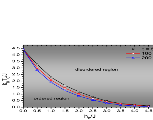
Dynamic phase diagram separating dynamically ordered and disordered phases of the thin film system in a plane in the absence of bias field is shown in Fig. 1 at various values. At first sight, it can be easily seen from the figure that, for a fixed value of , the system shows ordered phase at the relatively low temperature and applied field amplitude regions. Here, the time dependent magnetization of the system oscillate around a non-zero value, namely, the system may not respond to the external magnetic field instantaneously. With increasing strength of the amplitude of the external field, the magnetic phase of the system tends to shift dynamically paramagnetic phase. In this region, the time dependent magnetization of the thin film system oscillate around a zero value, and it can follow the external field with a relatively small phase lag depending on the studied system parameters. One of the obtained results of our MC simulation study is that the thin film system shows sensitivity to varying applied field period in accordance with the expectations. For a fixed value of , it is obvious that as is increased, the phase transition point is lowered because of the fact that decreasing field frequency leads to a decreasing phase delay between the magnetization and magnetic field and this makes the occurrence of the dynamic phase transition easy. The physical discussions mentioned above can be easily visualized by checking any two values of oscillation periods such as and for fixed value of .
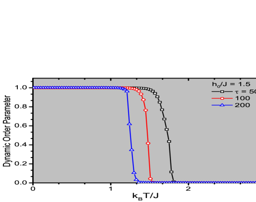
In Fig. 2 we present the thermal variations of dynamic order parameter of thin film system corresponding to phase diagrams plotted in Fig. 1 for various values with a selected applied field amplitude . It is evident from our simulation that when the temperature increases starting from zero, the dynamic order parameter starts to decrease from its saturation value, and it undergoes a second order dynamic phase transition between dynamically ordered and disordered phases. As we discussed above, dynamic phase transition point moves downward in the temperature space with increasing applied field period. It is possible to see more clearly these facts in this figure.
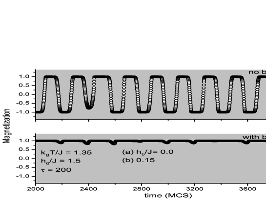
Before we start to discuss the influences of bias field on the thermal and magnetic behavior of the thin film system, it is beneficial to underline that there exists a competition between bias and time dependent magnetic fields. Namely, the bias field tries to keep the system in ordered phase whereas the time dependent magnetic field tries to drive the system into dynamically disordered phase depending on the other system parameters. From this point of view, in Fig. 3 (a) we give time series of the magnetization without a bias field for selected values of and . One can deduce from the figure that the unbiased magnetization curve displays a nearly rectangular shaped time sequence around zero value such that the thin film system exists in dynamically paramagnetic phase. As shown in Fig. 3(b), by keeping the system parameters fixed, if one applies the bias field to the thin film system, for example , the biased magnetization curve shows a small variation around its saturation value with increasing time. We should note that application of the bias field to the system is sufficient to induce a large value indicating the existence of an ordered phase, and it also allows us to analogy with static paramagnetic saturation at large applied field values. If one compares the our MC simulation findings with the experimental data in Fig. 2 of Ref. [28], a well agreement is seen between modeling and experiment.
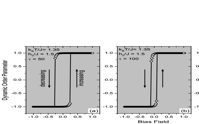
In the following analysis, we give the bias field dependencies of the dynamic order parameter for a fixed temperature and applied field amplitude for varying applied field periods in Fig. 4(a)-(c). The measurement procedure to obtain the decreasing branches of the hysteresis curves is as follows: The bias field starts at , and then it is slowly decreased with a step until it reaches to . We obtain the increasing branches of the curves using a similar way. The decreasing and increasing branches of the hysteresis curves are shown by downward and upward arrows in figures. One of the outstanding results is that dynamically ordered state is not simply inverted at , and therefore, hysteresis curve appears. When one compares the obtained curve with hysteresis curve for ferromagnetic system at thermal equilibrium, it may possible to say that bias field appears to be the conjugate field of the dynamic order parameter . Furthermore, the aforementioned behavior strongly depends on the applied field period, and it disappears with increasing value of the applied field period.
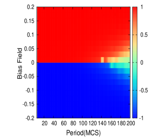
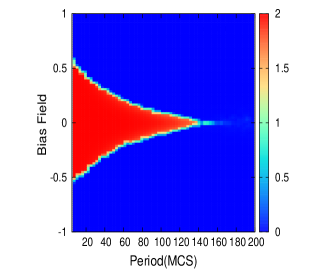
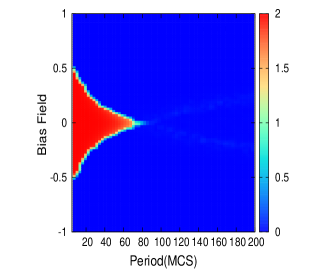
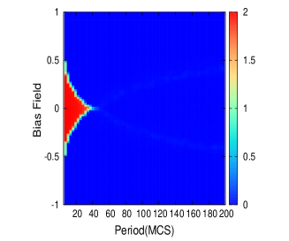
As a final investigation, we touch upon the period dependencies of dynamic hysteresis curve for a considered value of temperature with different values of the applied field amplitudes in Fig. (5). In order to generate the Fig. 5(a) constructed as a color-coded map displaying the stable dynamic order parameter as a function of the applied field period and bias field, we follow a similar way used in Ref. [28]. It is found that a sharp transition takes place at between positive and negative values up to a particular value of . With increasing value of starting from a relatively low value, vanishes at . As a result of this, the sharp transition behavior tends to disappear, and there is no phase transition line as reaches at a critical value. The curves in Figs. 5(b)-(d) are plotted for three values of applied field amplitude: (b) , (c) and (d) . The figures represent a map of . In other words, this formula determines the differences of the values obtained for the decreasing branch and the increasing branch . It is clear from the figures that the obtained curves appear as the roughly triangular structure extending up to a critical period value which sensitively depends on the applied field amplitude and other system parameters. When the energy coming from the time dependent applied field is increased, the boundaries of the triangular shapes tend to show a decreasing trend, and it is possible to mention that after a special value of the amplitude of field, the triangular shape completely disappears.
4 Conclusion
In summary, we have investigated the thermal and magnetic phase transition features of the ferromagnetic thin film system under the influence both bias field and time-dependent magnetic fields. For this purpose, we have used Monte Carlo simulation technique with single-spin flip Metropolis algorithm. First, to determine the dynamic phase transition point, we have treated the thermal variation of the heat capacity for considered values of the system parameters, and by benefiting from its peak, we have constructed the dynamic phase diagram in reduced magnetic field versus temperature plane. It is reported that for a fixed value of , as is increased, the phase transition point is lowered since decreasing field frequency gives rise to a decreasing phase delay between the magnetization and magnetic field and this makes the occurrence of the dynamic phase transition easy. Next, we have focused on effects of the varying bias field on the ferromagnetic thin film system, and we have studied the dynamic hysteresis behaviors as a functions of system parameters in detail. It is emphasized that is the conjugate field to the dynamic order parameter, and also appears to define a phase line between two antiparallel dynamic ordered states. As a final note, it should be underlined that our MC simulation results obtained in the present work corroborate the experimental observations found in Ref. [28].
5 Acknowledgements
The authors thank Andreas Berger from CIC Nanogune for critical reading of the manuscript and for valuable discussions on the subject. The numerical calculations reported in this paper were performed at TÜBİTAK ULAKBİM (Turkish agency), High Performance and Grid Computing Center (TRUBA Resources).
References
- [1] T. Tomé, M.J. de Oliveira, Dynamic phase transition in the kinetic Ising model under a time-dependent oscillating field, Phys. Rev. A 41 (1990) 4251.
- [2] M. Acharyya, Comparison of mean-field and Monte Carlo approaches to dynamic hysteresis in Ising ferromagnets, Physica A 253 (1998) 199.
- [3] G.M. Buendía, E. Machado, Kinetics of a mixed Ising ferrimagnetic system, Phys. Rev. E 58 (1998) 1260.
- [4] M. Keskin, E. Kantar, O. Canko, Kinetics of a mixed spin- and spin- Ising system under a time-dependent oscillating magnetic field, Phys. Rev. E 77 (2008) 051130.
- [5] O. Canko, E. Kantar, M. Keskin, Nonequilibrium phase transition in the kinetic Ising model on a two-layer square lattice under the presence of an oscillating field, Physica A 388 (2009) 28.
- [6] A. Punya, R. Yimnirun, P. Laoratanakul, Y. Laosiritaworn, Frequency dependence of the Ising hysteresis phase diagram: Mean field analysis, Physica B 405 (2010) 3488.
- [7] M. Ertaş, M. Keskin, Dynamic magnetic behavior of the mixed-spin bilayer system in an oscillating field within the mean-field theory, Phys. Lett. A 376 (2012) 2455.
- [8] X. Shi, G. Wei, L. Li, Effective-field theory on the kinetic Ising model, Phys. Lett. A 372 (2008) 5922.
- [9] B. Deviren, M. Keskin, Thermal behavior of dynamic magnetizations, hysteresis loop areas and correlations of a cylindrical Ising nanotube in an oscillating magnetic field within the effective-field theory and the Glauber-type stochastic dynamics approach, Phys. Lett. A 376 (2012) 1011.
- [10] M. Ertaş, Y. Kocakaplan, Dynamic behaviors of the hexagonal Ising nanowire, Phys. Lett. A 378 (2014) 845.
- [11] B.O. Aktaş, Ü. Akıncı, H. Polat, Critical phenomena in dynamical Ising-typed thin films by effective-field theory, Thin Solid Films 562 (2014) 680.
- [12] Y. Yüksel, E. Vatansever, Ü. Akıncı, H. Polat, Nonequilibrium phase transitions and stationary-state solutions of a three-dimensional random-field Ising model under a time-dependent periodic external field, Phys. Rev. E 85 (2012) 051123.
- [13] E. Vatansever, Ü. Akıncı, Y. Yüksel, H. Polat, Investigation of oscillation frequency and disorder induced dynamic phase transitions in a quenched-bond diluted Ising ferromagnet, J. Magn. Magn. Mater. 329 (2013) 14.
- [14] Ü. Akıncı, Y. Yüksel, E. Vatansever, H. Polat, Nonequilibrium steady state of the kinetic Glauber Ising model under a periodically time-varying magnetic field, Physica A 391 (2012) 5810.
- [15] M. Acharyya, Nonequilibrium phase transition in the kinetic Ising model: Is the transition point the maximum lossy point? Phys. Rev. E 58 (1998) 179.
- [16] M. Acharyya, Multiple dynamic transitions in an anisotropic Heisenberg ferromagnet driven by polarized magnetic field, Phys. Rev. E 69 (2004) 027105.
- [17] S.W. Sides, P.A. Rikvold, M.A. Novotny, Kinetic Ising model in an oscillating field: Finite-size scaling at the dynamic phase transition, Phys. Rev. Lett. 81 (1998) 834.
- [18] Y. Laosiritaworn, Monte Carlo simulation on thickness dependence of hysteresis properties in Ising thin-films, Thin Solid Films 517 (2009) 5189.
- [19] H. Park, M. Pleimling, Surface Criticality at a Dynamic Phase Transition, Phys. Rev. Lett. 109 (2012) 175703.
- [20] Y. Yüksel, E. Vatansever, H. Polat, Dynamic phase transition properties and hysteretic behavior of a ferrimagnetic core shell nanoparticle in the presence of a time dependent magnetic field, J. Phys.: Condens. Matter 24 (2012) 436004.
- [21] E. Vatansever, H. Polat, Monte Carlo investigation of a spherical ferrimagnetic core shell nanoparticle under a time dependent magnetic field, J. Magn. Magn. Mater. 343 (2013) 221.
- [22] E. Vatansever, H. Polat, Non-equilibrium dynamics of a ferrimagnetic core shell nanocubic particle, Physica A 394 (2014) 82.
- [23] D.T. Robb, P.A. Rikvold, A. Berger, M.A. Novotny, Conjugate field and fluctuation-dissipation relation for the dynamic phase transition in the two-dimensional kinetic Ising model, Phys. Rev. E 76 (2007) 021124.
- [24] D.T. Robb, Y.H. Xu, O. Hellwig, J. McCord, A. Berger, M.A. Novotny, P.A. Rikvold, Evidence for a dynamic phase transition in magnetic multilayers, Phys. Rev. B 78 (2008) 134422.
- [25] O. Idigoras, P. Vavassori, A. Berger, Mean field theory of dynamic phase transitions in ferromagnets, Physica B 407 (2012) 1377.
- [26] R.A. Gallardo, O. Idigoras, P. Landeros, A. Berger, Analytical derivation of critical exponents of the dynamic phase transition in the mean-field approximation, Phys. Rev. E 86 (2012) 051101.
- [27] Y. Yüksel, Monte Carlo study of magnetization dynamics in uniaxial ferromagnetic nanowires in the presence of oscillating and biased magnetic fields, Phys. Rev. E 91 (2015) 032149.
- [28] A. Berger, O. Idigoras, P. Vavassori, Transient behavior of the dynamically ordered phase in uniaxial cobalt films, Phys. Rev. Lett. 111 (2013) 190602.
- [29] K. Binder, Monte Carlo Methods in Statistical Physics (Springer, Berlin, 1979).
- [30] M.E.J. Newman, G.T. Barkema, Monte Carlo Methods in Statistical Physics (Oxford University Press, New York, 1999).