Information Without Rolling Dice

Abstract

The deterministic notions of capacity and entropy are studied in the context of communication and storage of information using square-integrable, bandlimited signals subject to perturbation. The $(\epsilon,\delta)$-capacity, that extends the Kolmogorov $\epsilon$-capacity to packing sets of overlap at most $\delta$, is introduced and compared to the Shannon capacity. The functional form of the results indicates that in both Kolmogorov and Shannon’s settings, capacity and entropy grow linearly with the number of degrees of freedom, but only logarithmically with the signal to noise ratio. This basic insight transcends the details of the stochastic or deterministic description of the information-theoretic model. For $\delta=0$, the analysis leads to new bounds on the Kolmogorov $\epsilon$-capacity, and to a tight asymptotic expression of the Kolmogorov $\epsilon$-entropy of bandlimited signals. A deterministic notion of error exponent is introduced. Applications of the theory are briefly discussed.

I Introduction

Claude Shannon introduced the notions of capacity and entropy in the context of communication in 1948 [1], and with them he ignited a technological revolution. His work instantly became a classic and it is today the pillar of modern digital technologies. On the other side of the globe, the great Soviet mathematician Andrei Kolmogorov was acquainted with Shannon’s work in the early 1950s and immediately recognized that “his mathematical intuition is remarkably precise.” His notions of $\epsilon$-entropy and $\epsilon$-capacity [2, 3] were certainly influenced by Shannon’s work. The $\epsilon$-capacity has the same operational interpretation of Shannon’s in terms of the limit for the amount of information that can be transmitted under perturbation, but it was developed in the purely deterministic setting of functional approximation. On the other hand, the $\epsilon$-entropy corresponds to the amount of information required to represent any function of a given class within $\epsilon$ accuracy, while the Shannon entropy corresponds to the average amount of information required to represent any stochastic process of a given class, quantized at level $\epsilon$. Kolmogorov’s interest in approximation theory dated back to at least the nineteen-thirties, when he introduced the concept of $N$-width to characterize the “massiveness” or effective dimensionality of an infinite-dimensional functional space [4]. This interest also eventually led him to the solution in the late nineteen-fifties, together with his student Arnold, of Hilbert’s thirteenth problem [5].

Even though they shared the goal of mathematically describing the limits of communication and storage of information, Shannon and Kolmogorov’s approaches to information theory have evolved separately. Shannon’s theory flourished in the context of communication, while Kolmogorov’s work impacted mostly mathematical analysis. Connections between their definitions of entropy have been pointed out in [6], and we discussed the relationship between capacities in our previous work [7]. The related concept of complexity and its relation to algorithmic information theory has been treated extensively [8, 9]. Kolmogorov devoted his presentation at the 1956 International Symposium on Information Theory [10], and Appendix II of his work with Tikhomirov [3] to explore the relationship with the probabilistic theory of information developed in the West, but limited the discussion “at the level of analogy and parallelism.” This is not surprising, given the state of affairs of the mathematics of functional approximation in the nineteen-fifties — at the time the theory of spectral decomposition of time-frequency limiting operators, needed for a rigorous treatment of continuous waveform channels, had yet to be developed by Landau, Pollack and Slepian [11, 12].

Renewed interest in deterministic models of information has recently been raised in the context of networked control theory [13, 14], and in the context of electromagnetic wave theory [15, 16, 17]. Motivated by these applications, in this paper we define the number of degrees of freedom, or effective dimensionality, of the space of bandlimited functions in terms of $N$-width, and study capacity and entropy in Kolmogorov’s deterministic setting. We also extend Kolmogorov’s capacity to packing sets of non-zero overlap, which allows a more detailed comparison with Shannon’s work.

I-A Capacity and packing

Shannon’s capacity is closely related to the problem of geometric packing “billiard balls” in high-dimensional space. Roughly speaking, each transmitted signal, represented by the coefficients of an orthonormal basis expansion, corresponds to a point in the space, and balls centered at the transmitted points represent the probability density of the uncertainty of the observation performed at the receiver. A certain amount of overlap between the balls is allowed to construct dense packings corresponding to codebooks of high capacity, as long as the overlap does not include typical noise concentration regions, and this allows to achieve reliable communication with vanishing probability of error. The more stringent requirement of communication with probability of error equal to zero leads to the notion of zero-error capacity [18], which depends only on the region of uncertainty of the observation, and not on its probabilistic distribution, and it can be expressed as the supremum of a deterministic information functional [14].

Similarly, in Kolmogorov’s deterministic setting communication between a transmitter and a receiver occurs without error, balls of fixed radius $\epsilon$ representing the uncertainty introduced by the noise about each transmitted signal are not allowed to overlap, and his notion of $2\epsilon$-capacity corresponds to the Shannon zero-error capacity of the $\epsilon$-bounded noise channel.

In order to represent a vanishing-error in a deterministic setting, we allow a certain amount of overlap between the $\epsilon$-balls. In our setting, a codebook is composed by a subset of waveforms in the space, each corresponding to a given message. A transmitter can select any one of these signals, that is observed at the receiver with perturbation at most $\epsilon$. If signals in the codebook are at distance less than $2\epsilon$ of each other, a decoding error may occur due to the overlap region between the corresponding $\epsilon$-balls. The total volume of the error region, normalized by the total volume of the $\epsilon$-balls in the codebook, represents a measure of the fraction of space where the received signal may fall and result in a communication error. The $(\epsilon,\delta)$-capacity is then defined as the logarithm base two of the largest number of signals that can be placed in a codebook having a normalized error region of size at most $\delta$. We provide upper and lower bounds on this quantity, when communication occurs using bandlimited, square-integrable signals, and introduce a natural notion of deterministic error exponent associated to it, that depends only on the communication rate, on $\epsilon$, on the signals’ bandwidth, and on the energy constraint. Our bounds become tight for high values of the signal to noise ratio, and their functional form indicates that capacity grows linearly with the number of degrees of freedom, but only logarithmically with the signal to noise ratio. This was Shannon’s original insight, revisited here in a deterministic setting.

For $\delta=0$ our notion of capacity reduces to the Kolmogorov $2\epsilon$-capacity, and we provide new bounds on this quantity. By comparing the lower bound for $\delta>0$ and the upper bound for $\delta=0$, we also show that a strict inequality holds between the corresponding values of capacity if the signal to noise ratio is sufficiently large. The analogous result in a probabilistic setting is that the Shannon capacity of the uniform noise channel is strictly greater than the corresponding zero-error capacity.

I-B Entropy and covering

Shannon’s entropy is closely related to the geometric problem of covering a high-dimensional space with balls of given radius. Roughly speaking, each source signal, modeled as a stochastic process, corresponds to a random point in the space, and by quantizing all coordinates of the space at a given resolution, Shannon’s entropy corresponds to the number of bits needed on average to represent the quantized signal. Thus, the entropy depends on both the probability distribution of the process, and the quantization step along the coordinates of the space. A quantizer, however, does not need to act uniformly on each coordinate, and can be more generally viewed as a discrete set of balls covering the space. The source signal is represented by the closest center of a ball covering it, and the distance to the center of the ball represents the distortion measure associated to this representation. In this setting, Shannon’s rate distortion function provides the minimum number of bits that must be specified per unit time to represent the source process with a given average distortion.

In Kolmogorov’s deterministic setting, the $\epsilon$-entropy is the logarithm of the minimum number of balls of radius $\epsilon$ needed to cover the whole space and, when taken per unit time, it corresponds to the Shannon rate-distortion function, as it also represents the minimum number of bits that must be specified per unit time to represent any source signal with distortion at most $\epsilon$. We provide a tight expression for this quantity, when sources are bandlimited, square-integrable signals. The functional form of our result shows that the $\epsilon$-entropy grows linearly with the number of degrees of freedom and logarithmically with the ratio of the norm of the signal to the norm of the distortion. Once again, this was Shannon’s key insight that remains invariant when subject to a deterministic formulation.

The leitmotiv of the paper is the comparison between deterministic and stochastic approaches to information theory, and the presentation is organized as follows: In Section II we informally describe our results, in section III we present our model rigorously, provide some definitions, recall results in the literature that are useful for our derivations, and present our technical approach. Section IV briefly discusses applications. Section V provides precise mathematical statements of our results, along with their proofs. A discussion of previous results and the computation of the error exponent in the deterministic setting appear in the Appendixes.

II Description of the results

We begin with an informal description of our results, that is placed on rigorous grounds in subsequent sections.

II-A Capacity

We consider one-dimensional, real, scalar waveforms of a single scalar variable and supported over an angular frequency interval $[-\Omega,\Omega]$. We assume that waveforms are square-integrable, and satisfy the energy constraint

$$\int_{-\infty}^{\infty}f^{2}(t)dt\leq E.$$ (1)

These bandlimited waveforms have unbounded time support, but are observed over a finite interval $[-T/2,T/2]$. In this way, and in a sense to be made precise below, any signal can be expanded in terms of a suitable set of basis functions, orthonormal over the real line, and for $T$ large enough it can be seen as a point in a space of essentially

$$N_{0}=\Omega T/\pi$$ (2)

dimensions, corresponding to the number of degrees of freedom of the waveform, and of radius $\sqrt{E}$.

To introduce the notion of capacity, we consider an uncertainty sphere of radius $\epsilon$ centered at each signal point, representing the energy of the noise that is added to the observed waveform. In this model, due to Kolmogorov, the signal to noise ratio is

$$\mbox{{SNR}}_{K}=E/\epsilon^{2}.$$ (3)

A codebook is composed by a subset of waveforms in the space, each corresponding to a given message. A transmitter can select any one of these signals, that is observed at the receiver with perturbation at most $\epsilon$. By choosing signals in the codebook to be at at distance at least $2\epsilon$ of each other, the receiver can decode the message without error. The $2\epsilon$-capacity is the logarithm base two of the maximum number $M_{2\epsilon}(E)$ of distinguishable signals in the space. This geometrically corresponds to the maximum number of disjoint balls of radius $\epsilon$ with their centers situated inside the signals’ space and it is given by

$$C_{2\epsilon}=\log M_{2\epsilon}(E)\;\;\;\mbox{bits}.$$ (4)

We also define the capacity per unit time

$$\bar{C}_{2\epsilon}=\lim_{T\rightarrow\infty}\frac{\log M_{2\epsilon}(E)}{T}\;\;\;\mbox{bits per second}.\$$ (5)

A similar Gaussian stochastic model, due to Shannon, considers bandlimited signals in a space of essentially $N_{0}$ dimensions, subject to an energy constraint over the interval $[-T/2,T/2]$ that scales linearly with the number of dimensions

$$\int_{-T/2}^{T/2}f^{2}(t)dt\leq PN_{0},$$ (6)

and adds a zero mean Gaussian noise variable of standard deviation $\sigma$ independently to each coordinate of the space. In this model, the signal to noise ratio on each coordinate is

$$\mbox{{SNR}}_{S}=P/\sigma^{2}.$$ (7)

Shannon’s capacity is the logarithm base two of the largest number of messages $M_{\sigma}^{\delta}(P)$ that can be communicated with probability of error $\delta>0$. When taken per unit time, this is

$$C=\lim_{T\rightarrow\infty}\frac{\log M_{\sigma}^{\delta}(P)}{T}\;\;\;\mbox{bits per second},$$ (8)

and it does not depend on $\delta$. The definition in (8) should be compared with (5). The geometric insight on which the two models are built upon is the same. However, while in Kolmogorov’s deterministic model packing is performed with “hard” spheres of radius $\epsilon$ and communication in the presence of arbitrarily distributed noise over a bounded support is performed without error, in Shannon’s stochastic model packing is performed with “soft” spheres of effective radius $\sqrt{N_{0}}\sigma$ and communication in the presence of Gaussian noise of unbounded support is performed with arbitrarily low probability of error $\delta$.

Shannon’s energy constraint (6) scales with the number of dimensions, rather than being a constant. The reason for this should be clear: since the noise is assumed to act independently on each signal’s coefficient, the statistical spread of the output, given the input signal, corresponds to an uncertainty ball of radius $\sqrt{N_{0}}\sigma$. It follows that the norm of the signal should also be proportional to $\sqrt{N_{0}}$, to avoid a vanishing signal to noise ratio as $N_{0}\rightarrow\infty$. In contrast, in the case of Kolmogorov the capacity is computed assuming an uncertainty ball of fixed radius $\epsilon$ and the energy constraint is constant. In both cases, spectral concentration ensures that the size of the signals’ space is essentially of $N_{0}$ dimensions. Probabilistic concentration ensures that the noise in Shannon’s model concentrates around its standard deviation, so that the functional form of the results is similar in the two cases.

Shannon’s celebrated formula for the capacity of the Gaussian model is [1]

$$C=\frac{\Omega}{\pi}\log(\sqrt{1+\mbox{{SNR}}_{S}})\;\;\;\mbox{bits per second}.$$ (9)

Our results for Kolmogorov’s deterministic model are

$$\bar{C}_{2\epsilon} \leq\frac{\Omega}{\pi}\log\left(1+\sqrt{\mbox{{SNR}}_{K}/2}\right)\;\;\;\mbox{bits per second},$$ (10)

$$\bar{C}_{2\epsilon} \geq\frac{\Omega}{\pi}\left(\log\sqrt{\mbox{{SNR}}_{K}}-1\right)\;\;\;\mbox{bits per second}.$$ (11)

The upper bound (10) is an improved version of our previous one in [7]. For high values of the signal to noise ratio, it becomes approximately $\Omega/\pi\left(\log\sqrt{\mbox{{SNR}}_{K}}-1/2\right)$, i.e. tight up to a term $\Omega/(2\pi)$. Both upper and lower bounds are improvements over the ones given by Jagerman [19, 20], see Appendix -C for a discussion.

To provide a more precise comparison between the deterministic and the stochastic model, we extend the deterministic model allowing signals in the codebook to be at distance less than $2\epsilon$ of each other. We say that signals in a codebook are $(\epsilon,\delta)$-distinguishable if the portion of space where the received signal may fall and result in a decoding error is of measure at most $\delta$. The $(\epsilon,\delta)$-capacity is the logarithm base two of the maximum number $M_{\epsilon}^{\delta}(E)$ of $(\epsilon,\delta)$-distinguishable signals in the space and it is given by

$$C_{\epsilon}^{\delta}=\log M_{\epsilon}^{\delta}(E)\;\;\;\mbox{bits}.$$ (12)

We also define the $(\epsilon,\delta)$-capacity per unit time

$$\bar{C}_{\epsilon}^{\delta}=\lim_{T\rightarrow\infty}\frac{\log M_{\epsilon}^{\delta}(E)}{T}\;\;\;\mbox{bits per second}.\$$ (13)

In this case, we show, for any $\epsilon,\delta>0$

$$\bar{C}_{\epsilon}^{\delta} \leq\frac{\Omega}{\pi}\log\left(1+\sqrt{\mbox{{SNR}}_{K}}\right)\;\;\;\mbox{bits per second},$$ (14)

$$\bar{C}_{\epsilon}^{\delta} \geq\frac{\Omega}{\pi}\log\sqrt{\mbox{{SNR}}_{K}}\;\;\;\mbox{bits per second}.$$ (15)

As in Shannon’s case, these results do not depend on the size of the error region $\delta$. They become tight for high values of the signal to noise ratio.

The lower bound follows from a random coding argument by reducing the problem to the existence of a coding scheme for a stochastic uniform noise channel with arbitrarily small probability of error. The existence of such a scheme in the stochastic setting implies the existence of a corresponding scheme in the deterministic setting as well. Comparing (10) and (15) it follows that in the high $\mbox{{SNR}}_{K}$ regime, where

$$\sqrt{E}>\frac{\sqrt{2}}{\sqrt{2}-1}\epsilon,$$ (16)

having a positive error region guarantees a strictly larger capacity. Given our proof reduction, this corresponds to having a Shannon capacity for the uniform noise channel strictly greater than the corresponding zero-error capacity.

The analogy between the size of the error region in the deterministic setting and the probability of error in the stochastic setting also leads to a notion of deterministic error exponent. Letting the number of messages in the codebook be $M=2^{TR}$, where the transmission rate $R$ is smaller than the lower bound (15), in Appendix -E we bound the size of the error region to be at most

$$\delta\leq 2^{-T\left(\frac{\Omega}{\pi}\log\scriptsize{\sqrt{\mbox{{SNR}}_{K}}}-R\right)},$$ (17)

and the error exponent in the deterministic model is

$$\mbox{{Er}}(R)=\frac{\Omega}{\pi}\log\sqrt{\mbox{{SNR}}_{K}}-R>0,$$ (18)

that depends only on $\Omega$, $E$, $\epsilon$, and on the transmission rate $R$.

II-B Entropy

We consider the same signal space as above, corresponding to points of essentially $N_{0}=\Omega T/\pi$ dimensions and contained in a ball of radius $\sqrt{E}$. A source codebook is composed by a subset of points in this space, and each codebook point is a possible representation for the signals that are within radius $\epsilon$ of itself. If the union of the $\epsilon$ balls centered at all codebook points covers the whole space, then any signal in the space can be encoded by its closest representation. The radius $\epsilon$ of the covering balls provides a bound on the largest estimation error between any source $f(t)$ and its codebook representation $\hat{f}(t)$. When signals are observed over a finite time interval $[-T/2,T/2]$, this corresponds to

$$d[f(t),\hat{f}(t)]=\int_{-T/2}^{T/2}[f(t)-\hat{f}(t)]^{2}dt\leq\epsilon^{2}.$$ (19)

Following the usual convention in the literature, we call this distortion measure noise, so that the signal to distortion ratio in this source coding model is again $\mbox{{SNR}}_{K}=\sqrt{E}/\epsilon$.

The Kolmogorov $\epsilon$-entropy is the logarithm base two of the minimum number $L_{\epsilon}(E)$ of $\epsilon$-balls covering the whole space and it is given by

$$H_{\epsilon}=\log L_{\epsilon}(E)\;\;\;\mbox{bits}.$$ (20)

We also define the $\epsilon$-entropy per unit time

$$\bar{H}_{\epsilon}=\lim_{T\rightarrow\infty}\frac{\log L_{\epsilon}(E)}{T}\;\;\;\mbox{bits per second}.\$$ (21)

An analogous Gaussian stochastic source model, due to Shannon, models the source signal as a white Gaussian stochastic process of constant power spectral density $P$ of support $[-\Omega,\Omega]$. This stochastic process has infinite energy, and finite average power

$$\mathds{E}(\mathsf{f}^{2}(t))=R_{\mathsf{f}}(0)=\frac{1}{2\pi}\int_{-\infty}^{\infty}S_{\mathsf{f}}(\omega)d\omega=\frac{P\Omega}{\pi},$$ (22)

where $R_{\mathsf{f}}$ and $S_{\mathsf{f}}$ are the autocorrelation and the power spectral density of $f(t)$, respectively. When observed over the interval $[-T/2,T/2]$, the process can be viewed as a random point having essentially $N_{0}$ independent Gaussian coordinates of zero mean and variance $P$, and of energy

$$\int_{-T/2}^{T/2}\mathds{E}(\mathsf{f}^{2}(t))dt=\frac{P\Omega T}{\pi}=PN_{0}.$$ (23)

A source codebook is composed by a subset of points in the space, and each codebook point is a possible representation for the stochastic process. The distortion associated to the representation of $f(t)$ using codebook point $\hat{f}(t)$ is defined in terms of mean-squared error

$$d[\mathsf{f}(t),\hat{\mathsf{f}}(t)]=\int_{-T/2}^{T/2}\mathds{E}[\mathsf{f}(t)-\hat{\mathsf{f}}(t)]^{2}dt.$$ (24)

Letting $L_{\sigma}(P)$ be the smallest number of codebook points that can be used to represent the source process with distortion at most $\sigma^{2}N_{0}$, the rate-distortion function is defined as

$$R_{\sigma}=\lim_{T\rightarrow\infty}\frac{\log L_{\sigma}(P)}{T}\;\;\;\mbox{bits per second}.$$ (25)

In this setting, Shannon’s formula for the rate distortion function of a Gaussian source is [1]

$$R_{\sigma}=\frac{\Omega}{\pi}\log(\sqrt{\mbox{{SNR}}_{S}})\;\;\;\mbox{bits per second}.$$ (26)

We show the corresponding result in Kolmogorov’s deterministic setting

$$\bar{H}_{\epsilon}=\frac{\Omega}{\pi}\log(\sqrt{\mbox{{SNR}}_{K}})\;\;\;\mbox{bits per second}.$$ (27)

Previously, Jagerman [19, 20] has shown

$$0\leq\bar{H}_{\epsilon}\leq\frac{\Omega}{\pi}\log\left(1+2\sqrt{\mbox{{SNR}}_{K}}\right),$$ (28)

see Appendix -C for a discussion. Our result in (27) can be derived by combining a theorem of Dumer, Pinsker and Prelov [21, Theorem 2], on the thinnest covering of ellipsoids in Euclidean spaces of arbitrary dimension, our Lemma 57, on the phase transition of the dimensionality of bandlimited square-integrable functions, and an approximation argument given in our Theorem 6. Instead, we provide a self-contained proof.

II-C Summary

Table I

TABLE I: Comparison of stochastic and deterministic models

	Stochastic	Deterministic
Transmitted Signal	$\int_{-T/2}^{T/2}f^{2}(t)dt\leq PN_{0}$	$\int_{-\infty}^{\infty}f^{2}(t)dt\leq E$
Additive Noise	$\mathds{E}\sum_{i=1}^{N_{0}}\mathsf{n}_{i}^{2}=N_{0}{\sigma}^{2}$	$\sum_{i=1}^{\infty}n_{i}^{2}\leq{\epsilon}^{2}$
Effective Dimensionality	$N_{0}=\Omega T/\pi$	$N_{0}=\Omega T/\pi$
Signal to Noise Ratio	$\mathsf{SNR}_{S}=P/\sigma^{2}$	$\mathsf{SNR}_{K}=E/\epsilon^{2}$
Max Cardinality of Codebook	$M_{\sigma}^{\delta}(P)$	$M_{\epsilon}^{\delta}(E)$
Capacity	$C=\frac{\Omega}{\pi}\log(\sqrt{1+\mbox{{SNR}}_{S}})$	$\frac{\Omega}{\pi}\log\sqrt{\mbox{{SNR}}_{K}}\leq{\bar{C}}_{\epsilon}^{\delta}\leq\frac{\Omega}{\pi}\log(1+\sqrt{\mbox{{SNR}}_{K}})$
Source Signal	$\int_{-T/2}^{T/2}\mathds{E}(\mathsf{f}^{2}(t))dt=PN_{0}$	$\int_{-\infty}^{\infty}f^{2}(t)dt\leq E$
Distortion	$d[\mathsf{f}(t),\hat{f}(t)]\leq N_{0}\sigma^{2}$	$d[\mathsf{f}(t),\hat{\mathsf{f}}(t)]\leq\epsilon^{2}$
Min Cardinality of Codebook	$L_{\sigma}(P)$	$L_{\epsilon}(E)$
Rate Distortion Function	$R_{\sigma}=\frac{\Omega}{\pi}\log\sqrt{\mbox{{SNR}}_{S}}$	${\bar{H}}_{\epsilon}=\frac{\Omega}{\pi}\log\sqrt{\mbox{{SNR}}_{K}}$

provides a comparison between results in the deterministic and in the stochastic setting. In the computation of capacity, a transmitted signal subject to a given energy constraint, is corrupted by additive noise. Due to spectral concentration, the signal has an effective number of dimensions $N_{0}$. In a deterministic setting, the noise represented by the deterministic coordinates $\{n_{i}\}$, can take any value inside a ball of radius $\epsilon$. In a stochastic setting, due to probabilistic concentration, the noise represented by the stochastic coordinates $\{\mathsf{n}_{i}\}$, can take values essentially uniformly at random inside a ball of effective radius $N_{0}\sigma^{2}$. In both cases, the maximum cardinality of the codebook used for communication depends on the error measure $\delta>0$, but the capacity in bits per unit time does not, and it depends only on the signal to noise ratio. The special case $\delta=0$ is treated separately, and it does not appear in the table. This corresponds to the Kolmogorov $2\epsilon$-capacity, and is the analog of the Shannon zero-error capacity of an $\epsilon$-bounded noise channel.

In the computation of the rate distortion function, a source signal is modeled as either an arbitrary, or stochastic process of given energy constraint. The distortion measure corresponds to the estimation error incurred when this signal is represented by an element of the source codebook. The minimum cardinality of the codebook used for representation depends on the distortion constraint, and so does the rate distortion function.

In both the deterministic and stochastic settings we have a tight asymptotic characterization of the rate distortion function, while we have bounds for the capacity in the deterministic setting that are tight only in the high $\textsf{SNR}_{K}$ regime. This is because distances in the probabilistic model are measured in terms of standard deviation, while they are measured in terms of $L^{2}[-T/2,T/2]$ norm in the deterministic model. The computation of capacity requires to sum the signal and the noise, and in the probabilistic model the norm of the sum of two signals can be expressed as the square root of the sum of their variances, leading to a tight expression. In the deterministic model, the norm of the sum of two signals can only be bounded, and this leads to a gap between upper and lower bounds that vanishes for high values of $\textsf{SNR}_{K}$. In the case of rate distortion, we do not need to compute the sum of two signals, and tight bounds are obtained in both settings.

III The signals’ space

We now describe the signals’ space rigorously, mention some classic results required for our derivations, introduce rigorous notions of capacity and entropy, and present the technical approach that we use in the proofs.

III-A Energy-constrained, bandlimited functions

We consider the set of one-dimensional, real, bandlimited functions

$$\mathcal{B}_{\Omega}=\{f(t):\mathcal{F}f(\omega)=0,\mbox{ for }|\omega|>\Omega\},$$ (29)

where

$$\mathcal{F}f(\omega)=\int_{-\infty}^{\infty}f(t)\exp(-j\omega t)dt,$$ (30)

and $j$ denotes the imaginary unit.

These functions are assumed to be square-integrable, and to satisfy the energy constraint (1). We equip them with the $L^{2}[-T/2,T/2]$ norm

$$\|f\|=\left(\int_{-\frac{T}{2}}^{\frac{T}{2}}f^{2}(t)dt\right)^{1/2}.$$ (31)

It follows that $(\mathcal{B}_{\Omega},\|\cdot\|)$ is a metric space, whose elemets are real, bandlimited functions, of infinite duration and observed over a finite interval $[-T/2,T/2]$. The elements of this space can be optimally approximated, in the sense of Kolmogorov, using a finite series expansion of a suitable basis set.

III-B Prolate spheroidal basis set

Given any $T,\Omega>0$, there exists a countably infinite set of real functions $\{\psi_{n}(t)\}_{n=1}^{\infty}$, called prolate spheroidal wave functions (PSWF), and a set of real positive numbers $1>\lambda_{1}>\lambda_{2}>\cdots$ with the following properties:

Property 1. The elements of $\{\lambda_{n}\}$ and $\{\psi_{n}\}$ are solutions of the Fredholm integral equation of the second kind

$$\lambda_{n}\psi_{n}(t)=\int_{-\frac{T}{2}}^{\frac{T}{2}}\psi_{n}(s)\frac{\sin\Omega(t-s)}{\pi(t-s)}ds.$$ (32)

Property 2. The elements of $\{\psi_{n}(t)\}$ have Fourier transform that is zero for $|\omega|>\Omega$.

Property 3. The set $\{\psi_{n}(t)\}$ is complete in $\mathcal{B}_{\Omega}$.

Property 4. The elements of $\{\psi_{n}(t)\}$ are orthonormal in $(-\infty,\infty)$

$$\int_{-\infty}^{\infty}\psi_{n}(t)\psi_{m}(t)dt=\begin{cases}1&n=m,\\ 0&\mbox{otherwise}.\end{cases}$$ (33)

Property 5. The elements of $\{\psi_{n}(t)\}$ are orthogonal in $\left(-\frac{T}{2},\frac{T}{2}\right)$

$$\int_{-\frac{T}{2}}^{\frac{T}{2}}\psi_{n}(t)\psi_{m}(t)dt=\begin{cases}\lambda_{n}&n=m,\\ 0&\mbox{otherwise}.\end{cases}$$ (34)

Property 6. The eigenvalues in $\{\lambda_{n}\}$ undergo a phase transition at the scale of $N_{0}=\Omega T/\pi$: for any $\alpha>0$

$${}\lim_{N_{0}\rightarrow\infty}\lambda_{\lfloor(1-\alpha)N_{0}\rfloor}=1,$$ (35)

$${}\lim_{N_{0}\rightarrow\infty}\lambda_{\lfloor(1+\alpha)N_{0}\rfloor}=0.$$ (36)

Property 7. The width of the phase transition can be precisely characterized: for any $k>0$

$${}\lim_{N_{0}\rightarrow\infty}\lambda_{\lfloor N_{0}+k\log(N_{0}\pi/2)\rfloor}=\frac{1}{1+e^{k\pi^{2}}}.$$ (37)

For an extended treatment of PSWF see [22]. The phase transition behavior of the eigenvalues is a key property related to the number of terms required for a satisfactory approximation of any square integrable bandlimited function using a finite basis set. Much of the theory was developed jointly by Landau, Pollack, and Slepian, see [12] for a review. The precise asymptotic behavior in (37) was finally proven by Landau and Widom [23], after a conjecture of Slepian supported by a non-rigorous computation [24].

III-C Approximation of $\mathcal{B}_{\Omega}$

Let $\mathcal{X}=L^{2}[-T/2,T/2]$, the Kolmogorov $N$-width [25] of $\mathcal{B}_{\Omega}$ in $\mathcal{X}$ is

$$d_{N}(\mathcal{B}_{\Omega},\mathcal{X})=\inf_{\mathcal{X}_{N}\subseteq\mathcal{X}}\sup_{f\in\mathcal{B}_{\Omega}}\inf_{g\in\mathcal{X}_{N}}\|f-g\|,$$ (38)

where $\mathcal{X}_{N}$ is an $N$-dimensional suspace of $\mathcal{X}$. For any $\mu>0$, we use this notion to define the number of degree of freedom at level $\mu$ of the space $\mathcal{B}_{\Omega}$ as

$$N_{\mu}(\mathcal{B}_{\Omega})=\min\{N:d_{N}(\mathcal{B}_{\Omega},\mathcal{X})\leq\mu\}.$$ (39)

In words, the Kolmogorov $N$-width represents the extent to which $\mathcal{B}_{\Omega}$ may be uniformly approximated by an $N$-dimensional subspace of $\mathcal{X}$, and the number of degrees of freedom is the dimension of the minimal subspace representing the elements of $\mathcal{B}_{\Omega}$ within the desired accuracy $\mu$. It follows that the number of degrees of freedom represents the effective dimensionality of the space, and corresponds to the number of coordinates that are essentially needed to identify any one element in the space.

A basic result in approximation theory (see e.g. [25, Ch. 2, Prop. 2.8]) states that

$${}d_{N}(\mathcal{B}_{\Omega},\mathcal{X})=\sqrt{E\lambda_{N+1}},$$ (40)

and the corresponding approximating subspace is the one spanned by the PSWF basis set $\{\psi_{n}\}_{n=1}^{N}$. It follows that any bandlimited function $f\in\mathcal{B}_{\Omega}$ can be optimally approximated by retaining a finite number $N$ of terms in the series expansion

$$f(t)=\sum_{n=1}^{\infty}b_{n}\psi_{n}(t),$$ (41)

and that the number of degree of freedom in (39) is given by the minimum index $N$ such that $\sqrt{\lambda_{N+1}}\leq\mu/\sqrt{E}$. The phase transition of the eigenvalues ensures that this number is only slightly larger than $N_{0}$. More precisely, for any $\mu>0$ we may choose an integer

$$N =N_{0}+\frac{1}{\pi^{2}}\log\left(\frac{E}{\mu^{2}}-1\right)\log\left(\frac{N_{0}\pi}{2}\right)+o(\log N_{0}),$$ (42)

and approximate

$$\mathcal{B}_{\Omega}=\left\{{\bf{b}}=(b_{1},b_{2},\cdots):\sum_{n=1}^{\infty}b_{n}^{2}\leq E\right\},$$ (43)

within accuracy $\mu$ as $N_{0}\rightarrow\infty$ using

$$\mathcal{B}_{\Omega}^{{}^{\prime}}=\left\{{\bf{b}}=(b_{1},b_{2},\cdots,b_{N}):\sum_{n=1}^{N}b_{n}^{2}\leq E\right\},$$ (44)

equipped with the norm

$$\|{\bf{b}}\|^{\prime}=\sqrt{\sum_{n=1}^{N}b_{n}^{2}\lambda_{n}}.$$ (45)

The energy constraint in (44) follows from (1) using the orthonormality Property 4 of the PSWF, the norm in (45) follows from (31) using the orthogonality Property 5 of the PSWF, and the desired level of approximation is guaranteed by Property 7 of the PSWF.

By (42) it follows that the number of degrees of freedom is an intrinsic property of the space, essentially dependent on the time-bandwidth product $N_{0}=\Omega T/\pi$, and only weakly, i.e. logarithmically, on the accuracy $\mu$ of the approximation and on the energy constraint $E$.

These approximation-theoretic results show that any energy-constrained, bandlimited waveform can be identified by essentially $N_{0}$ real numbers. This does not pose a limit on the amount of information carried by the signal. The real numbers identifying the waveform can be specified up to arbitrary precision, and this results in an infinite number of possible waveforms that can be used for communication. To bound the amount of information, we need to introduce a resolution limit at which the waveform can be observed, which allows an information-theoretic description of the space using bits rather than real numbers. This description is given in terms of entropy and capacity.

III-D $\epsilon$-entropy and $\epsilon$-capacity

Let $\mathcal{A}$ be a subset of the metric space $\mathcal{X}=L^{2}[-T/2,T/2]$. A set of points in $\mathcal{A}$ is called an $\epsilon$-covering if for any point in $\mathcal{A}$ there exists a point in the covering at distance at most $\epsilon$ from it. The minimum cardinality of an $\epsilon$-covering is an invariant of the set $\mathcal{A}$, which depends only on $\epsilon$, and is denoted by $L_{\epsilon}(\mathcal{A})$. The $\epsilon$-entropy of $\mathcal{A}$ is defined as the base two logarithm

$$H_{\epsilon}(\mathcal{A})=\log L_{\epsilon}(\mathcal{A})\;\;\;\mbox{bits},\$$ (46)

see Fig. 1-(a). We also define the $\epsilon$-entropy per unit time

$${\bar{H}}_{\epsilon}(\mathcal{A})=\lim_{T\rightarrow\infty}\frac{H_{\epsilon}(\mathcal{A})}{T}\;\;\;\mbox{bits per second}.\$$ (47)

A set of points in $\mathcal{A}$ is called $\epsilon$-distinguishable if the distance between any two of them exceeds $\epsilon$. The maximum cardinality of an $\epsilon$-distinguishable set is an invariant of the set $\mathcal{A}$, which depends only on $\epsilon$, and is denoted by $M_{\epsilon}(\mathcal{A})$. The $\epsilon$-capacity of $\mathcal{A}$ is defined as the base two logarithm

$$C_{\epsilon}(\mathcal{A})=\log M_{\epsilon}(\mathcal{A})\;\;\;\mbox{bits},\$$ (48)

see Fig. 1-(b). We also define the $\epsilon$-capacity per unit time

$${\bar{C}}_{\epsilon}(\mathcal{A})=\lim_{T\rightarrow\infty}\frac{C_{\epsilon}(\mathcal{A})}{T}\;\;\;\mbox{bits per second}.\$$ (49)

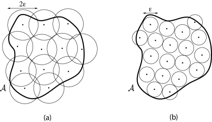
Figure 1: Part (a): Illustration of the $\epsilon$-entropy. Part (b): Illustration of the $\epsilon$-capacity.

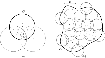
Figure 2: Part (a): Illustration of the error region for a signal in the space. The letters indicate the volume of the corresponding regions of the ball $\mathcal{S}^{1}$, and $\Delta_{1}=(c+e+f+g+i)/(a+b+c+d+e+f+g+h+i)$. Part (b): Illustration of the $(\epsilon,\delta)$-capacity. An overlap among the $\epsilon$-balls is allowed, provided that the cumulative error measure $\Delta\leq\delta$.

The $\epsilon$-entropy and $\epsilon$-capacity are closely related to the probabilistic notions of entropy and capacity used in information theory. The $\epsilon$-entropy corresponds to the rate distortion function, and the $\epsilon$-capacity corresponds to the zero-error capacity. In order to have a deterministic quantity that corresponds to the Shannon capacity, we extend the $\epsilon$-capacity and allow a small fraction of intersection among the $\epsilon$-balls when constructing a packing set. This leads to a certain region of space where the received signal may fall and result in a communication error, and to the notion of $(\epsilon,\delta)$-capacity.

III-E $(\epsilon,\delta)$-capacity

Let $\mathcal{A}$ be a subset of the metric space $\mathcal{X}=L^{2}[-T/2,T/2]$. We consider a set of points in $\mathcal{A}$, $\mathcal{M}=\{{\bf{a}}^{(1)},{\bf{a}}^{(2)},\cdots,{\bf{a}}^{(M)}\}$. For a given ${\bf{a}}^{(i)}$, $1\leq i\leq M$, we let the noise ball

$$\mathcal{S}^{i}=\{{\bf{x}}\in\mathcal{X}:\|{\bf{x}}-{\bf{a}}^{(i)}\|\leq\epsilon\},$$ (50)

where $\epsilon$ is a positive real number, and we let error region with respect to minimum distance decoding

$$\mathcal{D}^{i}=\{{\bf{x}}\in\mathcal{S}^{i}:\exists j\not=i:\|{\bf{x}}-{\bf{a}}^{(j)}\|\leq\|{\bf{x}}-{\bf{a}}^{(i)}\|\}.$$ (51)

We define the error measure for the $i$th signal

$$\Delta_{i}=\frac{{\rm{vol}}(\mathcal{D}^{i})}{{\rm{vol}}(\mathcal{S}^{i})},$$ (52)

where ${\rm{vol}(\cdot)}$ indicates volume in $\mathcal{X}$, and the cumulative error measure

$$\Delta=\frac{1}{M}\sum_{i=1}^{M}{\Delta_{i}},$$ (53)

Fig. 2-(a) provides an illustration of the error region for a signal in the space. Clearly, we have $0\leq\Delta\leq 1$. For any $\delta>0$, we say that a set of points $\mathcal{M}$ in $\mathcal{A}$ is $(\epsilon,\delta)$-distinguishable set if $\Delta\leq\delta$. The maximum cardinality of an $(\epsilon,\delta)$-distinguishable set is an invariant of the space $\mathcal{A}$, which depends only on $\epsilon$ and $\delta$, and is denoted by $M_{\epsilon}^{\delta}(\mathcal{A})$. The $(\epsilon,\delta)$-capacity of $\mathcal{A}$ is defined as the base two logarithm

$$C_{\epsilon}^{\delta}(\mathcal{A})=\log M_{\epsilon}^{\delta}(\mathcal{A})\;\;\;\mbox{bits},$$ (54)

see Fig. 2-(b). We also define the $(\epsilon,\delta)$-capacity per unit time

$$\bar{C}_{\epsilon}^{\delta}(\mathcal{A})=\lim_{T\rightarrow\infty}\frac{C_{\epsilon}^{\delta}({\mathcal{A}})}{T}\;\;\;\mbox{bits per second}.\$$ (55)

III-F Technical approach

Our objective is to compute entropy and capacity of square integrable, bandlimited functions. First, we perform this computation for the finite-dimensional space of functions $\mathcal{B}_{\Omega}^{{}^{\prime}}$ that approximates the infinite-dimensional space $\mathcal{B}_{\Omega}$ up to arbitrary accuracy $\mu>0$ in the $L^{2}[-T/2,T/2]$ norm, as $N_{0}\rightarrow\infty$. Our results in this setting are given by Theorem 1 for the $\epsilon$-capacity, Theorem 2 for the $(\epsilon,\delta)$-capacity, and Theorem 3 for the $\epsilon$-entropy. Then, in Theorems 4, 5, and 6, we extend the computation to the $\epsilon$-capacity, $(\epsilon,\delta)$-capacity, and $\epsilon$-entropy of the whole space $\mathcal{B}_{\Omega}$ of bandlimited functions.

When viewed per unit time, results for the two spaces are identical, indicating that using a highly accurate, lower-dimensional subspace approximation leaves only a negligible “information leak” in higher dimensions. We bound this leak in the case of $\epsilon$-entropy and $\epsilon$-capacity by performing a projection from the high-dimensional space $\mathcal{B}_{\Omega}$ onto the lower-dimensional one $\mathcal{B}_{\Omega}^{{}^{\prime}}$ and noticing that distances do not change significantly when these two spaces are sufficiently close to one another. On the other hand, for the $(\epsilon,\delta)$-capacity the error is defined in terms of volume, which may change significantly, no matter how close the two spaces are. In this case, we cannot bound the $(\epsilon,\delta)$ capacity of $\mathcal{B}_{\Omega}$ by performing a projection onto $\mathcal{B}_{\Omega}^{{}^{\prime}}$, and instead provide a bound on the capacity per unit time in terms of another finite-dimensional space that asymptotically approximates $\mathcal{B}_{\Omega}$ with perfect accuracy $\mu=0$, as $N_{0}\rightarrow\infty$.

IV Applications

Recent interest in deterministic models of information has been raised in the context of control theory and electromagnetic wave theory.

Control theory often treats uncertainties and disturbances as bounded unknowns having no statistical structure. In this context, Nair [14] introduced a maximin information functional for non-stochastic variables and used it to derive tight conditions for uniformly estimating the state of a linear time-invariant system over an error-prone channel. The relevance of Nair’s approach to estimation over unreliable channels is due to its connection with the Shannon zero-error capacity [14, Theorem 4.1], which has applications in networked control theory [13]. In Appendix -D we point out that Nairs’ maximum information rate functional, when viewed in our continuous setting of communication with bandlimited signals, is nothing else than $\bar{C}(\mathcal{B}_{\Omega})$. This suggests that our approach can be used in the same context as his.

In electromagnetic wave theory, the field measurement accuracy, and the corresponding image resolution in remote sensing applications, are often treated as fixed constants below which distinct electromagnetic fields, corresponding to different images, must be considered indistinguishable. In this framework, the number of degrees of freedom of radiating fields has been determined starting from their bandlimitation properties [26, 27]. Using the same approach, in communication theory the number of parallel channels available in spatially distributed multiple antenna systems under a fixed noise level constraint has been determined and related to the cut-set boundary separating transmitters and receivers [15]. Our results can be used in the same setting to provide the extension from the approximation-theoretic notion of degrees of freedom to the information-theoretic ones of entropy and capacity, something already suggested in [27].

Several other applications of the deterministic approach pursued here seem worth exploring, including the analysis of multi-band signals of sparse support. More generally, one could study capacity and entropy under different constrains beside bandlimitation, and attempt, for example, to obtain formulas analogous to waterfilling solutions in a deterministic setting.

V Nothing but proofs

We start with some preliminary lemmas that are needed for the proof of our main theorems. The first lemma is a consequence of the phase transition of the eigenvalues, while the second and third lemmas are properties of Euclidean spaces.

Lemma 1.

Let

$$\zeta(N)=\left(\prod_{i=1}^{N}\lambda_{i}\right)^{1/(2N)},$$ (56)

where $N=N_{0}+O(\log N_{0})$ as $N_{0}\rightarrow\infty$. We have

$$\lim_{N_{0}\rightarrow\infty}\zeta(N)=1.$$ (57)

Proof:

For any $\alpha>0$, we have

$$\log\zeta(N) =\frac{1}{2N}\sum_{i=1}^{N}\log\lambda_{i}$$

$$=\frac{1}{2N}\left(\sum_{i=1}^{\lfloor(1-\alpha)N_{0}\rfloor}\log\lambda_{i}\right.$$

$$\left.\hskip 19.91684pt+\sum_{i=\lfloor(1-\alpha)N_{0}\rfloor+1}^{N}\log\lambda_{i}\right).$$ (58)

From Property 6 of the PSWF and the monotonicity of the eigenvalues it follows that the first sum in (58) tends to zero as $N_{0}\rightarrow\infty$. We turn our attention to the second sum. By the monotonicity of the eigenvalues, we have

$$\sum_{i=\lfloor(1-\alpha)N_{0}+1\rfloor}^{N}\log\lambda_{i}\geq(N-(1-\alpha)N_{0})\log\lambda_{N}.$$ (59)

Since $N=N_{0}+O(\log N_{0})$ as $N_{0}\rightarrow\infty$, there exists a constant $k$ such that for $N_{0}$ large enough $N\leq N_{0}+k\log N_{0}$ and the right-hand side is an integer. It follows that for $N_{0}$ large enough, we have

$$\sum_{i=\lfloor(1-\alpha)N_{0}+1\rfloor}^{N}\log\lambda_{i} \geq(\alpha N_{0}+k\log N_{0})\log\lambda_{N}$$

$$\geq(\alpha N_{0}+k\log N_{0})$$

$$\times\log(\lambda_{N_{0}+k\log N_{0}}).$$ (60)

Substituting (60) into (58) and using Property 7 of the PSWF, it follows that for $N_{0}$ large enough

$$\log\zeta(N) \geq\frac{\alpha N_{0}+k\log N_{0}}{2N}\log\left(\frac{1}{1+e^{\pi^{2}k}}\right),$$ (61)

and since $N=N_{0}+O(\log N_{0})$ as $N_{0}\rightarrow\infty$, we have

$$\lim_{N_{0}\rightarrow\infty}\log\zeta(N)\geq\frac{\alpha}{2}\log\left(\frac{1}{1+e^{\pi^{2}k}}\right).$$ (62)

The proof is completed by noting that $\alpha$ can be arbitrarily small. ∎

Lemma 2.

Let $m$ be a positive integer and let ${\bf{x}},{\bf{x}}^{(1)},\cdots,{\bf{x}}^{(m)}$ be arbitrary points in $n$-dimensional Euclidean space, $(\mathbb{E}^{n}$, $\|\cdot\|)$. We have

$$\sum_{j=1}^{m}\sum_{k=1}^{m}\|{\bf{x}}^{(j)}-{\bf{x}}^{(k)}\|^{2}\leq 2m\sum_{j=1}^{m}\|{\bf{x}}-{\bf{x}}^{(j)}\|^{2}.$$ (63)

The proof is given in [28, Lemma 6.1].

Lemma 3.

Let $L$ be the cardinality of the minimal $\epsilon$-covering of the $\sqrt{E}$-ball $\mathcal{S}_{\sqrt{E}}$ in $\mathbb{E}^{n}$. If $n\geq 9$, we have

$$L\leq\frac{4e\cdot n^{3/2}\left(\frac{\sqrt{E}}{\epsilon}\right)^{n}}{\ln{n}-2}\left[n\cdot\ln{n}+o(n\cdot\ln{n})\right]$$ (64)

where $1<\frac{\sqrt{E}}{\epsilon}<\frac{n}{\ln{n}}$.

The proof is given in [29, Theorem 2].

V-A Main theorems for $\mathcal{B}_{\Omega}^{{}^{\prime}}$

Although the set $\mathcal{B}_{\Omega}^{{}^{\prime}}$ in (44) defines an $N$-dimensional hypersphere, the metric in (45) is not Euclidean. It is convenient to express the metric in Euclidean form by performing a scaling transformation of the coordinates of the space. For all $n$, we let $a_{n}=b_{n}\sqrt{\lambda_{n}}$, so that we have

$$\mathcal{B}_{\Omega}^{{}^{\prime}}=\left\{{\bf{a}}=(a_{1},a_{2},\cdots,a_{N}):\sum_{n=1}^{N}\frac{a_{n}^{2}}{\lambda_{n}}\leq E\right\}$$ (65)

and

$$\|{\bf{a}}\|^{\prime}=\sqrt{\sum_{n=1}^{N}a_{n}^{2}}.$$ (66)

We now consider packing and covering with $\epsilon$-balls inside the ellipsoid defined in (65), using the Euclidean metric in (66).

Theorem 1.

For any $\epsilon>0$, we have

$$\bar{C}_{\epsilon}^{0}(\mathcal{B}_{\Omega}^{{}^{\prime}})\geq\frac{\Omega}{\pi}\left[\log\left(\frac{\sqrt{E}}{\epsilon}\right)-1\right],$$ (67)

$$\bar{C}_{\epsilon}^{0}(\mathcal{B}_{\Omega}^{{}^{\prime}})\leq\frac{\Omega}{\pi}\left[\log\left(1+\frac{\sqrt{E}}{\epsilon\sqrt{2}}\right)\right].$$ (68)

Proof:

To prove the result it is enough to show the following inequalities for the $2\epsilon$-capacity

$$C_{\epsilon}^{0}(\mathcal{B}_{\Omega}^{{}^{\prime}})\geq N\left[\log\left(\zeta(N)\frac{\sqrt{E}}{\epsilon}\right)-1\right],$$ (69)

$$C_{\epsilon}^{0}(\mathcal{B}_{\Omega}^{{}^{\prime}})\leq N\left[\log\left(1+\frac{\sqrt{E}}{\sqrt{2}\epsilon}\right)\right]+\log\left(1+\frac{N}{2}\right),$$ (70)

because $\lim_{T\rightarrow\infty}\zeta(N)=1$ and $\log\left(1+\frac{N}{2}\right)=o(T)$.

Lower bound.    Let $\mathcal{M}_{\epsilon}^{0}$ be a maximal $(\epsilon,0)$-distinguishable subset of $\mathcal{B}_{\Omega}^{{}^{\prime}}$ and $M_{\epsilon}^{0}(\mathcal{B}_{\Omega}^{{}^{\prime}})$ be the number of elements in $\mathcal{M}_{\epsilon}^{0}$. For each point of $\mathcal{M}_{\epsilon}^{0}$, we consider an Euclidean ball whose center is the chosen point and whose radius is $2\epsilon$. Let $\mathcal{U}$ be the union of these balls. We claim that $\mathcal{B}_{\Omega}^{{}^{\prime}}$ is contained in $\mathcal{U}$. If that is not the case, we can find a point of $\mathcal{B}_{\Omega}^{{}^{\prime}}$ which is not contained in $\mathcal{M}_{\epsilon}^{0}$, but whose distance from every point in $\mathcal{M}_{\epsilon}^{0}$ exceeds $2\epsilon$, which is a contradiction. Thus, we have the chain of inequalities

$${\rm{vol}}(\mathcal{B}_{\Omega}^{{}^{\prime}})\leq{\rm{vol}}(\mathcal{U})\leq M_{\epsilon}^{0}(\mathcal{B}_{\Omega}^{{}^{\prime}}){\rm{vol}}(\mathcal{S}_{2\epsilon}),$$ (71)

where $\mathcal{S}_{2\epsilon}$ is an Euclidean ball whose radius is $2\epsilon$ and the second inequality follows from a union bound. Since ${\rm{vol}}(\mathcal{S}_{\epsilon})=\beta_{N}\cdot\epsilon^{N}$, where $\beta_{N}$ is the volume of $\mathcal{S}_{1}$, by (71) we have

$${\left(\frac{1}{2}\right)}^{N}\frac{{\rm{vol}}(\mathcal{B}_{\Omega}^{{}^{\prime}})}{{\rm{vol}}(\mathcal{S}_{\epsilon})}\leq M_{\epsilon}^{0}(\mathcal{B}_{\Omega}^{{}^{\prime}}).$$ (72)

Since $\mathcal{B}_{\Omega}^{{}^{\prime}}$ is an ellipsoid of radii $\{\sqrt{\lambda_{i}E}\}_{i=1}^{N}$, we also have

$${\rm{vol}}(\mathcal{B}_{\Omega}^{{}^{\prime}})=\beta_{N}\prod_{i=1}^{N}\sqrt{\lambda_{i}E}=\beta_{N}\left(\zeta(N)\sqrt{E}\right)^{N},$$ (73)

and

$$\frac{{{\rm{vol}}(\mathcal{B}_{\Omega}^{{}^{\prime}})}}{{{\rm{vol}}(\mathcal{S}_{\epsilon})}}=\left(\zeta(N)\frac{\sqrt{E}}{\epsilon}\right)^{N}.$$ (74)

By combining (72) and (74), we get

$$C_{\epsilon}^{0}(\mathcal{B}_{\Omega}^{{}^{\prime}})=\log M_{\epsilon}^{0}(\mathcal{B}_{\Omega}^{{}^{\prime}})\geq N\left[\log\left(\zeta(N)\frac{\sqrt{E}}{\epsilon}\right)-1\right].$$ (75)

Upper bound.    We define the auxiliary set

$$\bar{\mathcal{B}}_{\Omega}^{{}^{\prime}}=\left\{{\bf{a}}=(a_{1},a_{2},\cdots,a_{N}):\sum_{n=1}^{N}a_{n}^{2}\leq E\right\}.$$ (76)

The corresponding space $(\bar{\mathcal{B}}_{\Omega}^{{}^{\prime}},\|\cdot\|^{\prime})$ is Euclidean. Since $\mathcal{B}_{\Omega}^{{}^{\prime}}\subset\bar{\mathcal{B}}_{\Omega}^{{}^{\prime}}$, it follows that $C_{\epsilon}^{0}(\mathcal{B}_{\Omega}^{{}^{\prime}})\leq C_{\epsilon}^{0}(\bar{\mathcal{B}}_{\Omega}^{{}^{\prime}})$ and it is sufficient to derive an upper bound for $C_{\epsilon}^{0}(\bar{\mathcal{B}}_{\Omega}^{{}^{\prime}})$.

Let $\mathcal{M}_{\epsilon}^{0}=\{{\bf{a}}^{(1)},{\bf{a}}^{(2)},\cdots,{\bf{a}}^{(M)}\}$ be a maximal $(\epsilon,0)$-distinguishable subset of $\bar{\mathcal{B}}_{\Omega}^{{}^{\prime}}$, where $M=M_{\epsilon}^{0}(\bar{\mathcal{B}}_{\Omega}^{{}^{\prime}})$. Let $\{{\bf{a}}^{(i_{1})},{\bf{a}}^{(i_{2})}\cdots{\bf{a}}^{(i_{m})}\}$ be any subset of $\mathcal{M}_{\epsilon}^{0}$. For any integer $j\neq k$, $j,k\in\{1,\ldots m\}$, we have

$$\|{\bf{a}}^{(i_{j})}-{\bf{a}}^{(i_{k})}\|^{\prime}\geq 2\epsilon,$$ (77)

and

$$\sum_{j=1}^{m}\sum_{k=1}^{m}\|{\bf{a}}^{(i_{j})}-{\bf{a}}^{(i_{k})}\|^{\prime 2}\geq 4{\epsilon}^{2}m(m-1).$$ (78)

By Lemma 2 it follows that

$$\sum_{j=1}^{m}\|{\bf{a}}-{\bf{a}}^{(i_{j})}\|^{\prime 2}\geq 2{\epsilon}^{2}(m-1).$$ (79)

We now define the function

$$\gamma{(x)}=\max\{0,1-\frac{1}{2\epsilon^{2}}x^{2}\},$$ (80)

and for any ${\bf{a}}\in{\mathbb{E}}^{N}$, we let $\mathcal{M}_{\bf{a}}=\{{\bf{a}}^{(i_{1})},{\bf{a}}^{(i_{2})}\cdots{\bf{a}}^{(i_{m})}\}$ be a subset of $\mathcal{M}_{\epsilon}^{0}$ whose distance from ${\bf{a}}$ is not larger than $\sqrt{2}\epsilon$. We have

$$\sum_{j=1}^{M}\gamma(\|{\bf{a}}-{\bf{a}}^{(j)}\|^{\prime}) = \sum_{k=1}^{m}\gamma(\|{\bf{a}}-{\bf{a}}^{(i_{k})}\|^{\prime})$$ (81)

$$= \sum_{k=1}^{m}\left(1-\frac{1}{2\epsilon^{2}}\|{\bf{a}}-{\bf{a}}^{(i_{k})}\|^{\prime 2}\right)$$

$$= m-\frac{1}{2\epsilon^{2}}\sum_{k=1}^{m}\|{\bf{a}}-{\bf{a}}^{(i_{k})}\|^{\prime 2}$$

$$\leq m-(m-1)$$

$$= 1,$$

where the last inequality follows from (79). If ${\bf{a}}\notin\mathcal{S}_{\sqrt{E}+\sqrt{2}\epsilon}$, then $\sum_{j=1}^{M}\gamma(\|{\bf{a}}-{\bf{a}}^{(j)}\|^{\prime})=0$ because $\mathcal{M}_{\bf{a}}=\emptyset$. By using (81) and this last observation, we perform the following computation:

$${\rm{vol}}\left(\mathcal{S}_{\sqrt{E}+\sqrt{2}\epsilon}\right) = \int_{\mathcal{S}_{\sqrt{E}+\sqrt{2}\epsilon}}d{\bf{a}}$$ (82)

$$\geq \int_{\mathcal{S}_{\sqrt{E}+\sqrt{2}\epsilon}}\sum_{j=1}^{M}\gamma(\|{\bf{a}}-{\bf{a}}^{(j)}\|^{\prime})d{\bf{a}}$$

$$= \sum_{j=1}^{M}\int_{\mathbb{E}^{N}}\gamma(\|{\bf{a}}-{\bf{a}}^{(j)}\|^{\prime})d{\bf{a}}$$

$$= M\int_{\mathbb{E}^{N}}\gamma(\|{\bf{a}}\|^{\prime})d{\bf{a}}$$

$$= M\int_{0}^{\sqrt{2}\epsilon}\gamma(x)d(\beta_{N}x^{N})$$

$$= \beta_{N}MN\int_{0}^{\sqrt{2}\epsilon}\gamma(x)x^{N-1}dx$$

$$= \frac{2\beta_{N}M}{N+2}(\sqrt{2}\epsilon)^{N},$$

where $\beta_{N}$ is the volume of $\mathcal{S}_{1}$ in $\mathbb{E}^{N}$. Since ${\rm{vol}}\left(\mathcal{S}_{\sqrt{E}+\sqrt{2}\epsilon}\right)=\beta_{N}(\sqrt{E}+\sqrt{2}\epsilon)^{N}$, we obtain

$$M_{\epsilon}^{0}(\bar{\mathcal{B}}_{\Omega}^{{}^{\prime}})=M\leq\frac{N+2}{2}\left(1+\frac{\sqrt{E}}{\sqrt{2}\epsilon}\right)^{N}.$$ (83)

The proof is completed by taking the logarithm. ∎

Theorem 2.

For any $0<\delta<1$ and $\epsilon>0$, we have

$$\bar{C}_{\epsilon}^{\delta}(\mathcal{B}_{\Omega}^{{}^{\prime}})\geq\frac{\Omega}{\pi}\left[\log\left(\frac{\sqrt{E}}{\epsilon}\right)\right],$$ (84)

$$\bar{C}_{\epsilon}^{\delta}(\mathcal{B}_{\Omega}^{{}^{\prime}})\leq\frac{\Omega}{\pi}\left[\log\left(1+\frac{\sqrt{E}}{\epsilon}\right)\right].$$ (85)

Proof:

To prove the result it is enough to show the following inequalities for the $(\epsilon,\delta)$-capacity

$$C_{\epsilon}^{\delta}(\mathcal{B}_{\Omega}^{{}^{\prime}})\geq N\left[\log\left(\zeta(N)\frac{\sqrt{E}}{\epsilon}\right)\right]+\log{\delta},$$ (86)

$$C_{\epsilon}^{\delta}(\mathcal{B}_{\Omega}^{{}^{\prime}})\leq N\left[\log\left(1+\frac{\sqrt{E}}{\epsilon}\right)\right]+\log{\frac{1}{1-\delta}},$$ (87)

because $\lim_{T\rightarrow\infty}\zeta(N)=1$ and both $\log{\delta}$ and $\log{\frac{1}{1-\delta}}$ are $o(T)$.

Lower bound.    We show that there exists a codebook $\mathcal{M}=\{{\bf{a}}^{(1)},{\bf{a}}^{(2)},\cdots,{\bf{a}}^{(M)}\}$, where

$$M=\delta\left(\zeta(N)\frac{\sqrt{E}}{\epsilon}\right)^{N},$$ (88)

that has cumulative error measure $\Delta\leq\delta$. To prove this result, we consider an auxiliary stochastic communication model where the transmitter selects a signal uniformly at random from a given codebook and, given the signal ${\bf{a}}^{(i)}$ is sent, the receiver observes ${\bf{a}}^{(i)}+{\bf{n}}$, with ${\bf{n}}$ distributed uniformly in $\mathcal{S}_{\epsilon}$. The receiver compares this signal with all signals in the codebook and selects the one that is nearest to it as the one actually sent. The decoding error probability of this stochastic communication model, averaged over the uniform selection of signals in the codebook, is given by

$$P_{err}=\frac{1}{M}\sum_{i=1}^{M}\frac{{\rm{vol}}(\mathcal{D}^{i})}{{\rm{vol}}(\mathcal{S}^{i})},$$ (89)

and by (52) and (53) it corresponds to the cumulative error measure $\Delta$ of the deterministic model that uses the same codebook. It follows that in order to prove the desired lower bound in the deterministic model, we can show that there exists a codebook in the stochastic model satisfying (88), and whose decoding error probability is at most $\delta$. This follows from a standard random coding argument, in conjunction to a less standard geometric argument due to the metric employed.

We construct a random codebook by selecting $M$ signals uniformly at random inside the ellipsoid $\mathcal{B}_{\Omega}^{{}^{\prime}}$. We indicate the average error probability over all signal selections in the codebook and over all codebooks and by $\bar{P}_{err}$. Since all signals in the codebook have the same error probability when averaged over all codebooks, $\bar{P}_{err}$ is the same as the average error probability over all codebooks when ${\bf{a}}^{(1)}$ is transmitted. Let in this case the received signal be ${\bf{y}}$ and let $\mathcal{S}_{\epsilon}^{\bf{y}}$ be an Euclidean ball whose radius is $\epsilon$ and center is $\bf{y}$.

The probability that the signal $\bf{y}$ is decoded correctly is at least as large as the probability that the remaining $M-1$ signals in the codebook are in $\mathcal{B}_{\Omega}^{{}^{\prime}}\setminus\mathcal{S}_{\epsilon}^{\bf{y}}$. By the union bound, we have

$$1-\bar{P}_{err} \geq 1-(M-1)\frac{{\rm{vol}}(\mathcal{S}_{\epsilon}^{\bf{y}})}{{\rm{vol}}(\mathcal{B}_{\Omega}^{{}^{\prime}})}$$ (90)

$$\geq 1-M\frac{{\rm{vol}}(\mathcal{S}_{\epsilon}^{\bf{y}})}{{\rm{vol}}(\mathcal{B}_{\Omega}^{{}^{\prime}})}$$

$$= 1-M\left(\frac{\epsilon}{\zeta(N)\sqrt{E}}\right)^{N}.$$

Letting $M=\delta\left(\zeta(N)\frac{\sqrt{E}}{\epsilon}\right)^{N}$, we have $\bar{P}_{err}\leq\delta$. This implies that there exist a given codebook for which the average probability of error over the selection of signals in the codebook given in (89) is at most $\delta$. When this same codebook is applied in the deterministic model, we also have a cumulative error measure $\Delta\leq\delta$.

Upper bound.    Let $\mathcal{M}_{\epsilon}^{\delta}$ be a maximal $(\epsilon,\delta)$-distinguishable subset of $\mathcal{B}_{\Omega}^{{}^{\prime}}$ and $M_{\epsilon}^{\delta}(\mathcal{B}_{\Omega}^{{}^{\prime}})=M$ be the number of elements in $\mathcal{M}_{\epsilon}^{\delta}$. Let $\hat{\mathcal{B}}_{\Omega}^{{}^{\prime}}$ be the union of $\mathcal{B}_{\Omega}^{{}^{\prime}}$ and the trace of the inner points of an $\epsilon$-ball whose center is moved along the boundary of $\mathcal{B}_{\Omega}^{{}^{\prime}}$, as depicted in Fig. 3.

Figure 3: Illustration of the relationship between $\mathcal{B}_{\Omega}^{{}^{\prime}}$ and $\hat{\mathcal{B}}_{\Omega}^{{}^{\prime}}$.

Since $\bigcup_{i=1}^{M}{\mathcal{S}}^{i}\subset\hat{\mathcal{B}}_{\Omega}^{{}^{\prime}}$, we have

$${\rm{vol}}\left(\bigcup_{i=1}^{M}{\mathcal{S}}^{i}\right)\leq{\rm{vol}}\left(\hat{\mathcal{B}}_{\Omega}^{{}^{\prime}}\right).$$ (91)

Since $\bigcup_{i=1}^{M}{\mathcal{S}}^{i}=\biguplus_{i=1}^{M}({\mathcal{S}}^{i}\setminus{\mathcal{D}}^{i})$, where $\biguplus$ indicates disjoint union, we obtain

$${\rm{vol}}\left(\bigcup_{i=1}^{M}{\mathcal{S}}^{i}\right) = \sum_{i=1}^{M}\left[{\rm{vol}}({\mathcal{S}}^{i})-{\rm{vol}}({\mathcal{D}}^{i})\right]$$ (92)

$$= \sum_{i=1}^{M}{\rm{vol}}({\mathcal{S}}^{i})\left[1-\frac{{\rm{vol}}({\mathcal{D}}^{i})}{{\rm{vol}}({\mathcal{S}}^{i})}\right]$$

$$= \sum_{i=1}^{M}{\rm{vol}}({\mathcal{S}}^{i})\left(1-\Delta_{i}\right)$$

$$= M\cdot{\rm{vol}}({\mathcal{S}}_{\epsilon})(1-\Delta).$$

Since $\hat{\mathcal{B}}_{\Omega}^{{}^{\prime}}\subset\mathcal{S}_{\sqrt{E}+\epsilon}$, (91) can be rewritten as

$$M{\rm{vol}}({\mathcal{S}}_{\epsilon})(1-\Delta)\leq{\rm{vol}}\left(\mathcal{S}_{\sqrt{E}+\epsilon}\right)$$ (93)

or equivalently

$$M_{\epsilon}^{\delta}(\mathcal{B}_{\Omega}^{{}^{\prime}})=M\leq\frac{1}{1-\Delta}\left(1+\frac{\sqrt{E}}{\epsilon}\right)^{N}.$$ (94)

Since $C_{\epsilon}^{\delta}(\mathcal{B}_{\Omega}^{{}^{\prime}})=\log M_{\epsilon}^{\delta}(\mathcal{B}_{\Omega}^{{}^{\prime}})$ and $\Delta\leq\delta$, the result follows. ∎

Theorem 3.

For any $\epsilon>0$, we have

$$\bar{H}_{\epsilon}(\mathcal{B}_{\Omega}^{{}^{\prime}})=\frac{\Omega}{\pi}\left[\log\left(\frac{\sqrt{E}}{\epsilon}\right)\right].$$ (95)

Proof:

To prove the result it is enough to show the following inequalities for the $\epsilon$-entropy

$$H_{\epsilon}(\mathcal{B}_{\Omega}^{{}^{\prime}})\geq N\left[\log\left(\zeta(N)\frac{\sqrt{E}}{\epsilon}\right)\right],$$ (96)

$$H_{\epsilon}(\mathcal{B}_{\Omega}^{{}^{\prime}})\leq N\left[\log\left(\frac{\sqrt{E}}{\epsilon}\right)\right]+\eta(N),$$ (97)

where $\eta(N)=o(T)$ and $\lim_{T\rightarrow\infty}\zeta(N)=1$.

Lower bound.    Let $\mathcal{L}_{\epsilon}$ be a minimal $\epsilon$-covering subset of $\mathcal{B}_{\Omega}^{{}^{\prime}}$ and $L_{\epsilon}(\mathcal{B}_{\Omega}^{{}^{\prime}})$ be the number of elements in $\mathcal{L}_{\epsilon}$. Since $\mathcal{L}_{\epsilon}$ is an $\epsilon$-covering, we have

$${\rm{vol}}(\mathcal{B}_{\Omega}^{{}^{\prime}})\leq L_{\epsilon}(\mathcal{B}_{\Omega}^{{}^{\prime}}){\rm{vol}}(\mathcal{S}_{\epsilon}),$$ (98)

where $\mathcal{S}_{\epsilon}$ is an Euclidean ball whose radius is $\epsilon$. By combining (74) and (98), we have

$$L_{\epsilon}(\mathcal{B}_{\Omega}^{{}^{\prime}})\geq\left(\zeta(N)\frac{\sqrt{E}}{\epsilon}\right)^{N}.$$ (99)

The proof is completed by taking the logarithm.

Upper bound.    We define the auxiliary set

$$\bar{\mathcal{B}}_{\Omega}^{{}^{\prime}}=\left\{{\bf{a}}=(a_{1},a_{2},\cdots,a_{N}):\sum_{n=1}^{N}a_{n}^{2}\leq E\right\}.$$ (100)

The corresponding space $(\bar{\mathcal{B}}_{\Omega}^{{}^{\prime}},\|\cdot\|^{\prime})$ is Euclidean. Since $\mathcal{B}_{\Omega}^{{}^{\prime}}\subset\bar{\mathcal{B}}_{\Omega}^{{}^{\prime}}$, it follows that $H_{\epsilon}(\mathcal{B}_{\Omega}^{{}^{\prime}})\leq H_{\epsilon}(\bar{\mathcal{B}}_{\Omega}^{{}^{\prime}})$ and it is sufficient to derive an upper bound for $H_{\epsilon}(\bar{\mathcal{B}}_{\Omega}^{{}^{\prime}})$.

Let $\mathcal{L}_{\epsilon}$ be a minimal $\epsilon$-covering subset of $\bar{\mathcal{B}}_{\Omega}^{{}^{\prime}}$ and $L_{\epsilon}(\bar{\mathcal{B}}_{\Omega}^{{}^{\prime}})$ be the number of elements in $\mathcal{L}_{\epsilon}$. By applying Lemma 3, we have

$$L_{\epsilon}(\bar{\mathcal{B}}_{\Omega}^{{}^{\prime}})\leq\frac{4eN^{3/2}\left(\frac{\sqrt{E}}{\epsilon}\right)^{N}}{\ln{N}-2}\left[N\ln{N}+o(N\ln{N})\right],$$ (101)

for $N\geq 9$ and $1<\frac{\sqrt{E}}{\epsilon}<\frac{N}{\ln{N}}$. By taking the logarithm, we have

$$H_{\epsilon}(\bar{\mathcal{B}}_{\Omega}^{{}^{\prime}}) \leq N\log\left(\frac{\sqrt{E}}{\epsilon}\right)$$

$$\hskip 8.5359pt+\log\left(\frac{4eN^{3/2}}{\ln{N}-2}\left[N\ln{N}+o(N\ln{N})\right]\right),$$ (102)

Letting $\eta(N)$ be equal to the second term of (V-A) the result follows. ∎

V-B Main theorems for $\mathcal{B}_{\Omega}$

We now extend results to the full space $\mathcal{B}_{\Omega}$. We define the auxiliary set

$$\underline{\mathcal{B}}_{\Omega}=\left\{{\bf{b}}=(b_{1},\cdots,b_{N},0,0,\cdots):\sum_{n=1}^{N}b_{n}^{2}\leq E\right\}$$ (103)

whose norm is the same as $\mathcal{B}_{\Omega}$. We also use another auxiliary set

$$\mathcal{B}_{\Omega}^{{}^{\prime\prime}}=\left\{{\bf{b}}=(b_{1},b_{2},\cdots,b_{N^{\prime}}):\sum_{n=1}^{N^{\prime}}b_{n}^{2}\leq E\right\},$$ (104)

equipped with the norm

$$\|{\bf{b}}\|^{\prime\prime}=\sqrt{\sum_{n=1}^{N^{\prime}}b_{n}^{2}\lambda_{n}}.$$ (105)

where $N^{\prime}=(1+\alpha)N_{0}$ for an arbitrary $\alpha>0$.

Theorem 4.

For any $\epsilon>0$, we have

$$\bar{C}_{\epsilon}^{0}(\mathcal{B}_{\Omega})\geq\frac{\Omega}{\pi}\left[\log\left(\frac{\sqrt{E}}{\epsilon}\right)-1\right]$$ (106)

$$\bar{C}_{\epsilon}^{0}(\mathcal{B}_{\Omega})\leq\frac{\Omega}{\pi}\left[\log\left(1+\frac{\sqrt{E}}{\epsilon\sqrt{2}}\right)\right].$$ (107)

Proof:

By the continuity of the logarithmic function, to prove the upper bound it is enough to show that for any $\epsilon>\mu>0$

$$\bar{C}_{\epsilon}^{0}(\mathcal{B}_{\Omega})\leq\frac{\Omega}{\pi}\left[\log\left(1+\frac{\sqrt{E}}{(\epsilon-\mu)\sqrt{2}}\right)\right],$$ (108)

and in order to prove (106) and (108), it is enough to show the following inequalities for the $2\epsilon$-capacity: for any $\epsilon>\mu>0$

$$C_{\epsilon}^{0}(\mathcal{B}_{\Omega})\geq C_{\epsilon}^{0}(\mathcal{B}_{\Omega}^{{}^{\prime}}),$$ (109)

$$C_{\epsilon}^{0}(\mathcal{B}_{\Omega})\leq C_{\epsilon-\mu}^{0}(\mathcal{B}_{\Omega}^{{}^{\prime}}),$$ (110)

and then apply Theorem 1.

Lower bound.    Let $\mathcal{D}$ be a maximal $(\epsilon,0)$-distinguishable subset of $\mathcal{B}_{\Omega}$ whose cardinality is $2^{C_{\epsilon}^{0}(\mathcal{B}_{\Omega})}$. Similary, let $\mathcal{E}$ be a maximal $(\epsilon,0)$-distinguishable subset of $\underline{\mathcal{B}}_{\Omega}$ whose cardinality is $2^{C_{\epsilon}^{0}(\underline{\mathcal{B}}_{\Omega})}$. Note that $\mathcal{E}$ is also a $(\epsilon,0)$-distinguishable subset of $\mathcal{B}_{\Omega}$. Thus, we have

$$2^{C_{\epsilon}^{0}(\underline{\mathcal{B}}_{\Omega})}=|\mathcal{E}|\leq|\mathcal{D}|=2^{C_{\epsilon}^{0}(\mathcal{B}_{\Omega})}.$$ (111)

From which it follows that

$$C_{\epsilon}^{0}(\underline{\mathcal{B}}_{\Omega})\leq C_{\epsilon}^{0}(\mathcal{B}_{\Omega}).$$ (112)

Since $C_{\epsilon}^{0}(\underline{\mathcal{B}}_{\Omega})=C_{\epsilon}^{0}(\mathcal{B}_{\Omega}^{{}^{\prime}})$, the result follows.

Upper bound.    For any $\epsilon>\mu>0$, we consider a projection map $\beta_{\mu}:\mathcal{B}_{\Omega}\rightarrow\underline{\mathcal{B}}_{\Omega}$. Let $\mathcal{D}$ be a maximal $(\epsilon,0)$-distinguishable subset of $\mathcal{B}_{\Omega}$ whose cardinality is $2^{C_{\epsilon}^{0}(\mathcal{B}_{\Omega})}$. Similary, let $\mathcal{E}$ be a maximal $(\epsilon-\mu,0)$-distinguishable subset of $\underline{\mathcal{B}}_{\Omega}$ whose cardinality is $2^{C_{\epsilon-\mu}^{0}(\underline{\mathcal{B}}_{\Omega})}$.

We define $\mathcal{E^{\prime}}=\beta_{\mu}(\mathcal{D})$. In general, $\beta_{\mu}$ is not one-to-one correspondence, however $|\mathcal{D}|=|\mathcal{E^{\prime}}|$. If this is not the case, then there exist a pair of points ${\bf{b}}^{(1)},{\bf{b}}^{(2)}\in\mathcal{D}$ satisfying $\beta_{\mu}({\bf{b}}^{(1)})=\beta_{\mu}({\bf{b}}^{(2)})={\bf{a}}$, and we have

$$\|{\bf{b}}^{(1)}-{\bf{b}}^{(2)}\| =\|{\bf{b}}^{(1)}-{\bf{a}}+{\bf{a}}-{\bf{b}}^{(2)}\|$$

$$\leq\|{\bf{b}}^{(1)}-{\bf{a}}\|+\|{\bf{a}}-{\bf{b}}^{(2)}\|$$

$$\leq\mu+\mu$$

$$\leq 2\epsilon,$$ (113)

which is a contradiction. Thus, we have

$$2^{C_{\epsilon}^{0}(\mathcal{B}_{\Omega})}=|\mathcal{D}|=|\mathcal{E^{\prime}}|.$$ (114)

The distance between any pair of points in $\mathcal{E^{\prime}}$ exceeds $2(\epsilon-\mu)$. If this is not the case, then there exist a pair of points in $\mathcal{E^{\prime}}$ whose distance is smaller than $2(\epsilon-\mu)$. These two point can be represented by ${\bf{a}}^{(1)}=\beta_{\mu}({\bf{b}}^{(1)})$ and ${\bf{a}}^{(2)}=\beta_{\mu}({\bf{b}}^{(2)})$, where ${\bf{b}}^{(1)},{\bf{b}}^{(2)}\in\mathcal{D}$. It follows that

$$\|{\bf{b}}^{(1)}-{\bf{b}}^{(2)}\| =\|{\bf{b}}^{(1)}-{\bf{a}}^{(1)}+{\bf{a}}^{(1)}-{\bf{a}}^{(2)}+{\bf{a}}^{(2)}-{\bf{b}}^{(2)}\|$$

$$\leq\|{\bf{b}}^{(1)}-{\bf{a}}^{(1)}\|+\|{\bf{a}}^{(1)}-{\bf{a}}^{(2)}\|$$

$$\hskip 14.22636pt+\|{\bf{a}}^{(2)}-{\bf{b}}^{(2)}\|$$

$$\leq\mu+2(\epsilon-\mu)+\mu$$

$$\leq 2\epsilon,$$ (115)

which is a contradiction. Thus, $\mathcal{E^{\prime}}$ is a $(\epsilon-\mu,0)$-distingushiable subset of $\underline{\mathcal{B}}_{\Omega}$, and we have

$$|\mathcal{E^{\prime}}|\leq|\mathcal{E}|=2^{C_{\epsilon-\mu}^{0}(\underline{\mathcal{B}}_{\Omega})}.$$ (116)

By combinining (114) and (116), we obatin

$$2^{C_{\epsilon}^{0}(\mathcal{B}_{\Omega})}=|\mathcal{D}|=|\mathcal{E^{\prime}}|\leq|\mathcal{E}|=2^{C_{\epsilon-\mu}^{0}(\underline{\mathcal{B}}_{\Omega})}.$$ (117)

From which it follows that

$$C_{\epsilon}^{0}(\mathcal{B}_{\Omega})\leq C_{\epsilon-\mu}^{0}(\underline{\mathcal{B}}_{\Omega}).$$ (118)

Since $C_{\epsilon-\mu}^{0}(\underline{\mathcal{B}}_{\Omega})=C_{\epsilon-\mu}^{0}(\mathcal{B}_{\Omega}^{{}^{\prime}})$, the result follows.

∎

Theorem 5.

For any $0<\delta<1$ and $\epsilon>0$, we have

$$\bar{C}_{\epsilon}^{\delta}(\mathcal{B}_{\Omega})\geq\frac{\Omega}{\pi}\left[\log\left(\frac{\sqrt{E}}{\epsilon}\right)\right]$$ (119)

$$\bar{C}_{\epsilon}^{\delta}(\mathcal{B}_{\Omega})\leq\frac{\Omega}{\pi}\left[\log\left(1+\frac{\sqrt{E}}{\epsilon}\right)\right].$$ (120)

Proof:

In this case, while the lower bound follows from a corresponding inequality on the $(\epsilon,\delta)$-capacity, the upper bound follows from an approximation argument and holds for the $(\epsilon,\delta)$-capacity per unit time only.

Lower bound.    Let $\mathcal{E}$ be a maximal $(\epsilon,\delta^{\prime})$-distinguishable subset of $\mathcal{B}_{\Omega}^{{}^{\prime}}$ whose cardinality is $2^{C_{\epsilon}^{\delta^{\prime}}(\mathcal{B}_{\Omega}^{{}^{\prime}})}$. We define a map $\alpha:\mathcal{B}_{\Omega}^{{}^{\prime}}\rightarrow\mathcal{B}_{\Omega}$ such that, for ${\bf{b}}=(b_{1},\cdots,b_{N})\in\mathcal{B}_{\Omega}^{{}^{\prime}}$, we have

$$\alpha({\bf{b}})=(b_{1},\cdots,b_{N},0,0,\cdots)\in\mathcal{B}_{\Omega}.$$ (121)

Then $\alpha(\mathcal{E})$ is a $(\epsilon,\delta^{\prime\prime})$-distinguishable subset of $\mathcal{B}_{\Omega}$ where $\delta^{\prime\prime}\rightarrow 0$ for $\delta^{\prime}\rightarrow 0$. Thus, we can choose $\delta^{\prime}$ whose corresponding $\delta^{\prime\prime}$ is smaller than $\delta$. In this case, we have

$$2^{C_{\epsilon}^{\delta^{\prime}}(\mathcal{B}_{\Omega}^{{}^{\prime}})}=|\mathcal{E}|\leq 2^{C_{\epsilon}^{\delta^{\prime\prime}}(\mathcal{B}_{\Omega})}.$$ (122)

Also, since $\delta^{\prime\prime}<\delta$, we have

$$C_{\epsilon}^{\delta^{\prime\prime}}(\mathcal{B}_{\Omega})\leq C_{\epsilon}^{\delta}(\mathcal{B}_{\Omega}).$$ (123)

By combining (122) and (123), we obtain

$$C_{\epsilon}^{\delta^{\prime}}(\mathcal{B}_{\Omega}^{{}^{\prime}})\leq C_{\epsilon}^{\delta}(\mathcal{B}_{\Omega}).$$ (124)

The result now follows from Theorem 2.

Upper bound.    We define

$$d(\mathcal{B}_{\Omega}^{{}^{\prime\prime}},\mathcal{B}_{\Omega})=\sup_{f\in\mathcal{B}_{\Omega}}\inf_{g\in\mathcal{B}_{\Omega}^{{}^{\prime\prime}}}\|f-g\|$$ (125)

which is a measure of distance between $\mathcal{B}_{\Omega}^{{}^{\prime\prime}}$ and $\mathcal{B}_{\Omega}$. From the Property 6 of the PSWF, we have

$$d(\mathcal{B}_{\Omega}^{{}^{\prime\prime}},\mathcal{B}_{\Omega})\rightarrow 0\;\;\;\mbox{as}\;\;\;N_{0}\rightarrow\infty.$$ (126)

which implies

$$\bar{C}_{\epsilon}^{\delta}(\mathcal{B}_{\Omega})=\bar{C}_{\epsilon}^{\delta}(\mathcal{B}_{\Omega}^{{}^{\prime\prime}}).$$ (127)

Thus, in order to prove the upper bound of $\bar{C}_{\epsilon}^{\delta}(\mathcal{B}_{\Omega})$, it is sufficient to derive an upper bound for $\bar{C}_{\epsilon}^{\delta}(\mathcal{B}_{\Omega}^{{}^{\prime\prime}})$.

By using a the same proof technique as the one in Theorem 2, we obatin

$$C_{\epsilon}^{\delta}(\mathcal{B}_{\Omega}^{{}^{\prime\prime}})\leq N^{\prime}\left[\log\left(1+\frac{\sqrt{E}}{\epsilon}\right)\right]+\log{\frac{1}{1-\delta}}$$ (128)

which implies

$$\bar{C}_{\epsilon}^{\delta}(\mathcal{B}_{\Omega}^{{}^{\prime\prime}})\leq(1+\alpha)\frac{\Omega}{\pi}\left[\log\left(1+\frac{\sqrt{E}}{\epsilon}\right)\right].$$ (129)

Since $\alpha$ is an arbitrary positive number, the result follows.

∎

Theorem 6.

For any $\epsilon>0$, we have

$$\bar{H}_{\epsilon}(\mathcal{B}_{\Omega})=\frac{\Omega}{\pi}\left[\log\left(\frac{\sqrt{E}}{\epsilon}\right)\right].$$ (130)

Proof:

By the continuity of the logarithmic function, to prove the result it is enough to show that for any $\epsilon>\mu>0$

$$\bar{H}_{\epsilon}(\mathcal{B}_{\Omega})\geq\frac{\Omega}{\pi}\left[\log\left(\frac{\sqrt{E}}{\epsilon}\right)\right],$$ (131)

$$\bar{H}_{\epsilon}(\mathcal{B}_{\Omega})\leq\frac{\Omega}{\pi}\left[\log\left(\frac{\sqrt{E}}{\epsilon-\mu}\right)\right],$$ (132)

and in order to prove (131) and (132), it is enough to show the following inequalities for the $\epsilon$-entropy: for any $\epsilon>\mu>0$

$$H_{\epsilon}(\mathcal{B}_{\Omega})\geq H_{\epsilon}(\mathcal{B}_{\Omega}^{{}^{\prime}})$$ (133)

$$H_{\epsilon}(\mathcal{B}_{\Omega})\leq H_{\epsilon-\mu}(\mathcal{B}_{\Omega}^{{}^{\prime}}),$$ (134)

and then apply Theorem 3.

Lower bound.    For any $\epsilon>\mu>0$, we condiser a projection map $\beta_{\mu}:\mathcal{B}_{\Omega}\rightarrow\underline{\mathcal{B}}_{\Omega}$. Let $\mathcal{D}$ be a minimal $\epsilon$-covering subset of $\mathcal{B}_{\Omega}$ whose cardinality is $2^{H_{\epsilon}(\mathcal{B}_{\Omega})}$. Similary, let $\mathcal{E}$ be a minimal $\epsilon$-covering subset of $\underline{\mathcal{B}}_{\Omega}$ whose cardinality is $2^{H_{\epsilon}(\underline{\mathcal{B}}_{\Omega})}$.

We define $\mathcal{E^{\prime}}=\beta_{\mu}(\mathcal{D})$. We claim that $\mathcal{E^{\prime}}$ is also a $\epsilon$-covering subset of $\underline{\mathcal{B}}_{\Omega}$. Let ${\bf{p}}$ be a point of $\underline{\mathcal{B}}_{\Omega}$. Since $\mathcal{D}$ is an $\epsilon$-covering subset of $\mathcal{B}_{\Omega}$ and $\underline{\mathcal{B}}_{\Omega}\subset\mathcal{B}_{\Omega}$, there exists a point ${\bf{b}}\in\mathcal{D}$ such that $\|{\bf{b}}-{\bf{p}}\|\leq\epsilon$. Note that $\|\beta_{\mu}({\bf{b}})-{\bf{p}}\|\leq\|{\bf{b}}-{\bf{p}}\|$ and $\beta_{\mu}({\bf{b}})\in\mathcal{E^{\prime}}$. This means that, for any point ${\bf{p}}\in\underline{\mathcal{B}}_{\Omega}$, there exists a point in $\mathcal{E^{\prime}}$ whose distance from ${\bf{p}}$ is eqaul or less than $\epsilon$, which implies $\mathcal{E^{\prime}}$ is a $\epsilon$-covering subset of $\underline{\mathcal{B}}_{\Omega}$. Thus, we have

$$|\mathcal{E^{\prime}}|\geq|\mathcal{E}|=2^{H_{\epsilon}(\underline{\mathcal{B}}_{\Omega})}.$$ (135)

Since $|\mathcal{D}|\geq|\mathcal{E^{\prime}}|$, we obtain the following chain of inequlities:

$$2^{H_{\epsilon}(\mathcal{B}_{\Omega})}=|\mathcal{D}|\geq|\mathcal{E^{\prime}}|\geq|\mathcal{E}|=2^{H_{\epsilon}(\underline{\mathcal{B}}_{\Omega})}.$$ (136)

From which it follows that

$$H_{\epsilon}(\underline{\mathcal{B}}_{\Omega})\leq H_{\epsilon}(\mathcal{B}_{\Omega}).$$ (137)

Since $H_{\epsilon}(\underline{\mathcal{B}}_{\Omega})=H_{\epsilon}(\mathcal{B}_{\Omega}^{{}^{\prime}})$, the result follows.

Upper bound.    Let $\mathcal{D}$ be a minimal $\epsilon$-covering subset of $\mathcal{B}_{\Omega}$ whose cardinality is $2^{H_{\epsilon}(\mathcal{B}_{\Omega})}$. Similary, let $\mathcal{E}$ be a minimal $(\epsilon-\mu)$-covering subset of $\underline{\mathcal{B}}_{\Omega}$ whose cardinality is $2^{H_{\epsilon-\mu}(\underline{\mathcal{B}}_{\Omega})}$.

We claim that $\mathcal{E}$ is also an $\epsilon$-covering subset of $\mathcal{B}_{\Omega}$. Let ${\bf{p}}$ be a point of $\mathcal{B}_{\Omega}$. Since $\mathcal{E}$ is an $(\epsilon-\mu)$-covering subset of $\underline{\mathcal{B}}_{\Omega}$ and $\beta_{\mu}({\bf{p}})\in\underline{\mathcal{B}}_{\Omega}$, there exists a point ${\bf{a}}\in\mathcal{E}$ such that $\|{\bf{a}}-\beta_{\mu}({\bf{p}})\|\leq\epsilon-\mu$. Then,

$$\|{\bf{a}}-{\bf{p}}\| =\|{\bf{a}}-\beta_{\mu}({\bf{p}})+\beta_{\mu}({\bf{p}})-{\bf{p}}\|$$

$$\leq\|{\bf{a}}-\beta_{\mu}({\bf{p}})\|+\|\beta_{\mu}({\bf{p}})-{\bf{p}}\|$$

$$\leq\epsilon-\mu+\mu$$

$$=\epsilon.$$ (138)

This means that, for any point ${\bf{p}}\in\mathcal{B}_{\Omega}$, there exists a point in $\mathcal{E}$ whose distance from ${\bf{p}}$ is eqaul or less than $\epsilon$, which implies $\mathcal{E}$ is an $\epsilon$-covering subset of $\mathcal{B}_{\Omega}$. Thus, we have

$$2^{H_{\epsilon-\mu}(\underline{\mathcal{B}}_{\Omega})}=|\mathcal{E}|\geq|\mathcal{D}|=2^{H_{\epsilon}(\mathcal{B}_{\Omega})}.$$ (139)

From which it follows that

$$H_{\epsilon-\mu}(\underline{\mathcal{B}}_{\Omega})\geq H_{\epsilon}(\mathcal{B}_{\Omega}).$$ (140)

Since $H_{\epsilon-\mu}(\underline{\mathcal{B}}_{\Omega})=H_{\epsilon-\mu}(\mathcal{B}_{\Omega}^{{}^{\prime}})$, the result follows.

∎

-C Comparison with Jagerman’s results

A basic relationship between $\epsilon$-entropy and $\epsilon$-capacity, given in [3], is

$${}C_{2\epsilon}(\mathcal{A})\leq H_{\epsilon}(\mathcal{A}).$$ (141)

It follows that a typical technique to estimate entropy and capacity is to find a lower bound for $C_{2\epsilon}$ and an upper bound for $H_{\epsilon}$, and if these are close to each other, then they are good estimates for both capacity and entropy.

Following this approach, Jagerman provided a lower bound on the $2\epsilon$-capacity and an upper bound on the $\epsilon$-entropy of bandlimited functions. In our notation, the lower bound [19, Theorem 6] can be written as

$$C_{2\epsilon}\geq N_{0}\log\left(\frac{2}{\sqrt{10}}\sqrt{\frac{\mbox{{SNR}}_{K}}{N_{0}}}+1\right),$$ (142)

where the result is adapted here to real signals.

Jagerman’s proof roughly follows the codebook construction corresponding to the lattice packing depicted in Figure 4.

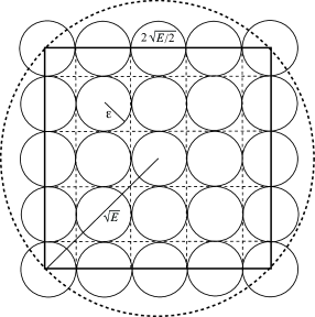
Figure 4: Lattice packing in Jagerman’s lower bound.

In higher dimensions the side length of the hypercube corresponding to the square in Figure 4 becomes $2\sqrt{E/N_{0}}$, which divided by the diameter $2\epsilon$ of the noise sphere gives the leading term $\sqrt{\mbox{{SNR}}_{K}/N_{0}}$ inside the logarithm. The precise result requires a more detailed analysis of the asymptotic dimensionality of the space. This lower bound becomes very loose as $N_{0}\rightarrow\infty$. In this case, by using the Taylor expansion of $\log(1+x)$ for $x$ near zero in (142), it follows that $C_{2\epsilon}$ grows only as $\sqrt{N_{0}}$ and, as a consequence, we have the trivial lower bound on the $2\epsilon$-capacity per unit time

$$\bar{C}_{2\epsilon}\geq 0.$$ (143)

Geometrically, this is due to the volume of the high-dimensional sphere tending to concentrate on its boundary. For this reason, the packing in the inscribed hypercube in Figure 4 captures only a vanishing fraction of the volume available in the sphere. In contrast, our lower bound in Theorem 1 is non-constructive, and it gives the correct scaling order of the number of bits that can be reliably communicated over the channel, namely $N_{0}$ rather than $\sqrt{N_{0}}$, yielding a non-trivial lower bound on the $2\epsilon$-capacity per unit time.

In the same paper, Jagerman derives an upper bound on the $\epsilon$-entropy [19, Theorem 8] by applying Mitjagin’s theorem [30], which relates entropy to the Kolmogorov $N$-width. This standard technique is also illustrated in [31, Theorem 8]. For bandlimited signals, Jagerman further improves Mityagin’s bound in a subsequent paper [20, Theorem 1], obtaining in our notation

$$H_{\epsilon}\leq N\log\left(\frac{2\sqrt{E}}{\epsilon-\mu}+\frac{\epsilon+\mu}{\epsilon-\mu}\right),$$ (144)

where $0<\mu<\epsilon$ and $N$ is defined in (42). Since $\mu$ is an arbitrary positive number, (144) can be approximated by

$$H_{\epsilon}\leq N\log\left(2\sqrt{\mbox{{SNR}}_{K}}+1\right).$$ (145)

The $\epsilon$-entropy per unit time is then bounded as

$$\bar{H}_{\epsilon}\leq\frac{\Omega}{\pi}\log(2\sqrt{\mbox{{SNR}}_{K}}+1).$$ (146)

By combining (141),(143) and (146), Jagerman obtains

$$0\leq\bar{H}_{\epsilon}\leq\frac{\Omega}{\pi}\log\left(2\sqrt{\mbox{{SNR}}_{K}}+1\right),$$ (147)

while we provide a tight characterization of the same quantity in Theorem 6 of this paper. If we use this tight result to bound the $2\epsilon$-capacity using the classic approach of (141), we obtain

$$\bar{C}_{2\epsilon}\leq\frac{\Omega}{\pi}\log\sqrt{\mbox{{SNR}}_{K}},$$ (148)

while our direct bounds given in Theorem 1 yield, for high values of $\mbox{{SNR}}_{K}$,

$$\frac{\Omega}{\pi}(\log\sqrt{\mbox{{SNR}}_{K}}-1)\leq\bar{C}_{2\epsilon}\leq\frac{\Omega}{\pi}(\log\sqrt{\mbox{{SNR}}_{K}}-1/2).$$ (149)

-D Relationship with Nair’s work

Nair defined the peak maximum information rate $R_{*}$ in [14, Lemma 4.2] and showed $R_{*}$ equals the zero-error capacity [14, Theorem 4.1]. In his paper, Nair defined $R_{*}$ for a discrete time channel, but this definition can be modified for a continuous time channel as follows:

$$R_{*}=\lim_{T\rightarrow\infty}\sup_{X:X\subset\mathcal{B}_{\Omega}}\frac{I_{*}(X;Y)}{T},$$ (150)

where $Y$ is the uncertain output signal yielded by $X$.

When we consider our channel model, it is clear that the supremum is achieved when $X$ is a maximal $2\epsilon$-distinguishable set, $\mathcal{M}_{2\epsilon}$. In this case, $I_{*}(X;Y)=\log|{X}|=\log{M_{2\epsilon}(\mathcal{B}_{\Omega})}$. Thus (150) can be rewritten as follows:

$$R_{*}=\lim_{T\rightarrow\infty}\frac{\log M_{2\epsilon}(\mathcal{B}_{\Omega})}{T}.$$ (151)

The right-hand side of (151) is the definition of ${\bar{C}}_{2\epsilon}(\mathcal{B}_{\Omega})$. Thus, we conclude that ${\bar{C}}_{2\epsilon}(\mathcal{B}_{\Omega})$ is a peak maximum information rate and equals the zero-error capacity in our setting.

-E Derivation of the error exponent

By (90), we have

$$\Delta=P_{err}\leq M\left(\frac{\epsilon}{\zeta(N)\sqrt{E}}\right)^{N}.$$ (152)

Let $M=2^{TR}$, where the transmission rate $R$ is smaller than the lower bound on ${\bar{C}}_{\epsilon}^{\delta}$. Then, (152) can be rewritten as

$$\Delta=P_{err}\leq 2^{-T\left[\frac{N}{T}\log\left(\zeta(N)\frac{\sqrt{E}}{\epsilon}\right)-R\right]}.$$ (153)

In a stochastic setting the error exponent is defined as the logarithm of the error probability. It follows that we may also define the error exponent in our deterministic model

$$\mbox{{Er}}(R)=\frac{N}{T}\log\left(\zeta(N)\frac{\sqrt{E}}{\epsilon}\right)-R.$$ (154)

Since $N/T$ tends to ${\Omega}/{\pi}$ and $\zeta(N)$ tends to $1$ as $T\rightarrow\infty$ , we can approximate the error exponent when $N_{0}$ is sufficiently large by

$$\mbox{{Er}}(R)=\frac{\Omega}{\pi}\log\left(\frac{\sqrt{E}}{\epsilon}\right)-R.$$ (155)

Aknowledgments. The question of determining a notion of error exponent in a deterministic setting was raised by Francois Baccelli, following the presentation of [7].

References

- [1] C. Shannon, “A mathematical theory of communication,” Bell Systems Technical Journal, vol. 27, pp. 379–423, 1948.
- [2] A. N. Kolmogorov, “On certain asymptotic characteristics of completely bounded metric spaces,” Uspekhi Matematicheskikh Nauk, 108(3), pp. 385–388, 1956. (In Russian)
- [3] A. N. Kolmogorov, V. M. Tikhomirov, “-entropy and -capacity of sets in functional spaces,” Uspekhi Matematicheskikh Nauk, 14(2), pp. 3–86, 1959. English translation: American Mathematical Society Translation Series, 2(17), pp. 277–364, 1961.
- [4] A. N. Kolmogorov, “ Über die beste Annäherung von Funktionen einer gegebenen Funktionenklasse. ”Annals of Mathematics 37(1), pp. 107-110, 1936. (In German).
- [5] A. N. Kolmogorov, “On the representation of continuous functions of many variables by superposition of continuous functions of one variable and addition.” Doklady Akademii Nauk SSSR, 114, pp. 953-956, 1957. (In Russian).
- [6] D. L. Donoho, “Wald lecture I: counting bits with Shannon and Kolmogorov , Technical Report, Stanford University, 2000.
- [7] T. J. Lim, M. Franceschetti, “A deterministic view on the capacity of bandlimited functions.” Proceedings of the 52nd Annual Allerton Conference on Communication, Control, and Computing, Monticello, Illinois, September 2014.
- [8] T. M. Cover, J. Thomas, “Elements of information theory.” Second edition. J. Wiley and sons, 2006.
- [9] T. M. Cover, P. Gacs, R. Gray, “Kolmogorov’s contributions to information theory and algorithmic complexity.” The Annals of Probability, 17(3), pp. 840-865, 1989.
- [10] A. N. Kolmogorov, “On the Shannon theory of information transmission in the case of continuous signals.” IRE Transactions on Information Theory, 2(4), pp.102-108, December 1956.
- [11] D. Slepian, “On Bandwidth.” Proceedings of the IEEE, 64(3), pp. 292-300, March 1976.
- [12] D. Slepian, “Some comments on Fourier analysis, uncertainty and modeling,” SIAM Review, vol. 25, no. 3, pp. 379–393, 1983.
- [13] A. S. Matveev and A. V. Savkin, “Shannon zero-error capacity in the problems of state estimation and stabilization via noisy communication channels.” International Journal of Control, 80, pp. 241–255, 2007.
- [14] G. Nair, “A non-stochastic information theory for communication and state estimation,” IEEE Transactions on automatic control, vol. 58, pp. 1497–1510, 2013.
- [15] M. Franceschetti, “On Landau’s eigenvalue theorem and its applications.” Proceedings of the IEEE International Symposium of Information Theory, Honolulu, Hawaii, July 2014. Extended version available on-line: “On Landau’s eigenvalue theorem and information cut-sets” http://arxiv.org/abs/1405.1761.
- [16] M. Franceschetti, M. D. Migliore, P. Minero, and F. Schettino, “The degrees of freedom of wireless networks via cut-set integrals.” IEEE Transactions on Information Theory, 57(11), pp. 3067-3079, 2011.
- [17] M. Franceschetti, M. D. Migliore, and P. Minero, “The capacity of wireless networks: information-theoretic and physical limits.” IEEE Transactions on Information Theory, 55(8), pp. 3413–3424, 2009.
- [18] C. Shannon, “The zero-error capacity of a noisy channel,” IRE Transactions on Information Theory, 2(3), pp. 8–19, 1956.
- [19] D. Jagerman, “-entropy and approximation of bandlimted functions,” SIAM Journal of Applied Mathematics., vol. 17, no. 2, pp. 362–376, 1969.
- [20] D. Jagerman, “Information theory and approximation of bandlimted functions,” Bell Systems Technical Journal, 49(8), pp. 1911–1941, 1970.
- [21] I. Dumer, M. S. Pinsker and V. V. Prelov, “On coverings of ellipsoids in Eucliden spaces.” IEEE Transactions on Information Theory, 50(10), pp. 2348–2356, 2004.
- [22] C. Flammer, “Spheroidal wave functions,” Stanford University Press, 1957. Reprinted 2005, Dover.
- [23] H. J. Landau, H. Widom, “The eigenvalue distribution of time and frequency limiting,” Journal of Mathematical Analysis and Applications, vol. 77, pp. 469–481, 1980.
- [24] D. Slepian. “Some asymptotic expansions for prolate spheroidal wave functions.” Journal of mathematics and physics, 44, pp. 99-140, 1965.
- [25] A. Pinkus, “-Widths in Approximation Theory,” Springer-Verlag, 1985.
- [26] O. Bucci, G. Franceschetti. On the spatial bandwidth of scattered fields. IEEE Trans. on Antennas and Propagation, 35(12), pp. 1445-1455, December 1985.
- [27] O. Bucci, G. Franceschetti. On the degrees of freedom of scattered fields. IEEE Trans. on Antennas and Propagation, 37(7), pp. 918-926, July 1989.
- [28] C. Zong, Sphere Packings, Springer, 2013.
- [29] C. A. Rogers, ”Covering a sphere with spheres”, Mathematika, 10, pp. 157–164, 1963.
- [30] B. S. Mitjagin. “The approximative dimension and bases in nuclear spaces,” Uspekhi Matematicheskikh Nauk, 16(4), pp. 63-132, 1961. English translation: Russian Mathematical Surveys. 16(4). pp. 59-127, 1961.
- [31] G. Lorentz, “Approximation of Functions,” AMS Chelsea Publishing, second edition, 1986.