SymPix: A spherical grid for efficient sampling of rotationally invariant operators

Abstract

We present SymPix, a special-purpose spherical grid optimized for efficient sampling of rotationally invariant linear operators. This grid is conceptually similar to the Gauss-Legendre (GL) grid, aligning sample points with iso-latitude rings located on Legendre polynomial zeros. Unlike the GL grid, however, the number of grid points per ring varies as a function of latitude, avoiding expensive over-sampling near the poles and ensuring nearly equal sky area per grid point. The ratio between the number of grid points in two neighbouring rings is required to be a low-order rational number (3, 2, 1, 4/3, 5/4 or 6/5) to maintain a high degree of symmetries. Our main motivation for this grid is to solve linear systems using multi-grid methods, and to construct efficient preconditioners through pixel-space sampling of the linear operator in question. The GL grid is not suitable for these purposes due to its massive over-sampling near the poles, leading to nearly degenerate linear systems, while HEALPix, another commonly used spherical grid, exhibits few symmetries, and is therefore computationally inefficient for these purposes. As a benchmark and representative example, we compute a preconditioner for a linear system with both HEALPix and SymPix that involves the operator $\widehat{\mathbf{D}}+\widehat{\mathbf{B}}^{T}\mathbf{N}^{-1}\widehat{\mathbf{B}}$, where $\widehat{\mathbf{B}}$ and $\widehat{\mathbf{D}}$ may be described as both local and rotationally invariant operators, and $\mathbf{N}$ is diagonal in pixel domain. For a bandwidth limit of $\ell_{\text{max}}=3000$, we find that SymPix, due to its higher number of internal symmetries, yields average speed-ups of 360 and 23 for $\widehat{\mathbf{B}}^{T}\mathbf{N}^{-1}\widehat{\mathbf{B}}$ and $\widehat{\mathbf{D}}$, respectively, relative to HEALPix.

1. Introduction

Unlike the plane, it is impossible to construct a regular discretization of the sphere. Instead, every conceivable spherical grid comes with its own set of trade-offs, emphasizing one or more features at the cost of others. Thus, there is no such thing as a perfect spherical grid, but the optimal grid instead depends sensitively on the application under consideration.

In this paper, we will restrict our attention to high-resolution grids designed for fast and accurate spherical harmonic transforms (SHTs). In such cases, the primary consideration is that the grid must allow for efficient $\mathcal{O}(\ell_{\text{max}}^{3})$ SHTs, where $\ell_{\text{max}}$ denotes the upper harmonic space bandwidth limit of the field in question, as opposed to the $\mathcal{O}(\ell_{\text{max}}^{4})$ scaling resulting from naive brute-force summation. This requires the use of Fast Fourier Transforms (FFTs) in the longitudinal direction, which in turn implies that i) sample points must be placed on a set of iso-latitude rings, and ii) sample points within each ring must be equidistant. However, there is still flexibility in choosing the latitude of each ring ($\theta_{j}\in[0,\pi]$), the number of grid points along each ring ($n_{j}$), and the initial offset of each ring ($\phi_{0,j}$).

Three popular spherical grids are the equiangular grid, the Gauss-Legendre grid (e.g., Doroshkevich et al., 2005), and HEALPix (Górski et al., 2005). Of these, the equiangular grid is the most straightforward, simply defined by evenly spaced grid points $(\theta_{i},\phi_{i})$ in both directions. This grid is typically used for geographical maps, and it is therefore also called a geographical grid.

Similarly, the standard Gauss-Legendre grid has a constant number of grid points per ring. However, the ring latitudes $\theta_{j}$ are defined such that $P_{N_{\text{rings}}}(\cos\theta_{j})=0$, where $P_{n}$ is the Legendre polynomial of degree $n$. This simple modification allows efficient spherical harmonic analysis to machine precision, and the grid is thus optimized for spherical harmonics transforms.

Both of these grids suffers from a massive over-sampling of the polar regions ($\theta$ close to $0$ or $\pi$) compared to the equatorial region ($\theta\approx\pi/2$), and this renders them sub-optimal, and sometimes even useless, for certain practical applications. An important example is the solution of discretized and bandwidth limited linear systems. If there is a large number of sample points within the correlation length implied by $\ell_{\text{max}}$, the system becomes degenerate and numerically unstable. Grids with nearly constant pixel areas perform much better than grids with strongly varying pixel areas for this type of applications.

One example of such grids is HEALPix, which is short for “Hierarchical Equal Area and Latitude Pixelization”. This grid has by construction both constant area pixel area per pixel and grid points located on iso-latitude, and is as such a good general-purpose grid. However, this generality comes at a cost in terms of spherical harmonics precision, as well as a low level of internal pixel symmetries.

The latter point is particularly important for our applications. Consider a function of two grid points, $\hat{n}_{1}$ and $\hat{n}_{2}$, that is both localized and rotationally invariant,

$$f(\hat{n}_{1},\hat{n}_{2})=\left\{\begin{array}[]{ll}f(\hat{n}_{1}\cdot\hat{n}_{2})&\text{if $\text{arccos}(\hat{n}_{1}\cdot\hat{n}_{2})<k\Delta$}\\ 0&\text{otherwise},\end{array}\right.$$ (1)

where $\Delta$ denotes the average distance between two neighbouring grid points. Thus, $f$ is assumed identically zero if the two grid points are separated by more than $k$ grid units. In our applications, which employ multi-grid and/or preconditioning methods, we need to evaluate $f$ for all relevant pairs $(\hat{n}_{1},\hat{n}_{2})$. Furthermore, because $f$ typically is computationally expensive, it is important to minimize the total number of function evaluations, and large speed-ups can be gained by exploiting symmetries and caching.

For HEALPix, $f$ needs to be evaluated $\mathcal{O}(k^{2}N_{\text{pix}})$ times, because the angular distances between neighbouring grid points are all different, up to handful of overall symmetries. In contrast, for the equi-angular and Gauss-Legendre grids only $\mathcal{O}(k^{2}\sqrt{N_{\text{pix}}})$ evaluations are needed. Since the number of grid points is constant for every ring, we only need to evaluate $f$ for the first grid point on every ring, accounting for all its neighbours, after which all function evaluations along the same ring will be given by symmetry.

In this paper, we construct a novel spherical grid called SymPix that combines the spherical harmonics transform precision of the Gauss-Legendre grid with the nearly uniform sample point distances of HEALPix, while at the same time maintaining a high degree symmetries within each ring, ensuring that fully sampling $f(\hat{n_{1}}\cdot\hat{n_{2}})$ scales as $\mathcal{O}(k^{2}\sqrt{N_{\text{pix}}})$.

2. The SymPix grid

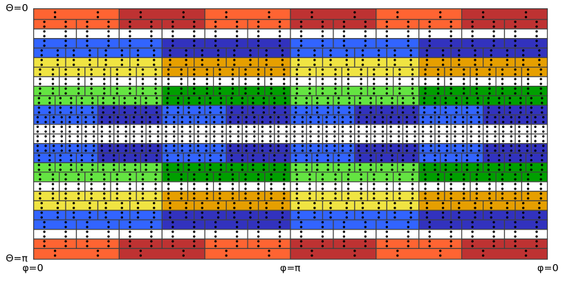
Figure 1.— Geometric layout of SymPix sample points, implementing a cylindrical projection of the sphere. Each rectangle indicates a tile of (in this case) $2\times 2$ sample points. For white tile-bands, the bands above and below have the same number of tiles, and angular distances between sample points in a given tile and sample points in the neighbouring tiles are therefore constant throughout the band. Function evaluations depending only on angular distances may therefore be cached and reused. Colored tile-bands increment the number of tiles by a factor of $2$ (red), $4/3$ (blue), $5/4$ (yellow), $6/5$ (green), and $4/3$ again (blue) towards the equator. For these bands, the neighbouring tile relationship repeats itself (as indicated by shading), and there are still only a few cases that need to be computed and cached for each band.

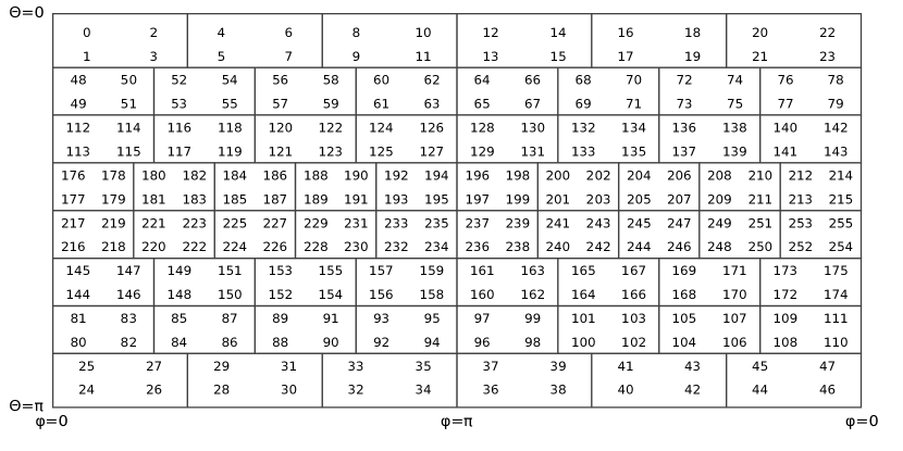
Figure 2.— Memory ordering of SymPix sample points. Note that the resolution is lower than in Figure 1. Within each band the pixel order increases first latitudinally, i.e., along the $\theta$ direction. This ensures that access within the same tile is local in memory, and there are no discontinuities along each ring, which is convenient for SHTs. Additionally, to support efficient distributed programming, we interleave Northern and Southern bands, such that they naturally are assigned to the same node without explicit additional book-keeping.

2.1. Ring layout basics

The main role of the SymPix grid is that of a supporting grid in internal multi-grid and/or preconditioning calculations, and maintaining high numerical precision is therefore essential. For this reason, we adopt the Gauss-Legendre latitudinal ring layout as the basis of our grid. This provides support for both spherical harmonic synthesis (i.e., transforming from harmonic coefficients to pixel space) and analysis (transforming from pixel space to harmonic coefficients) to machine precision, by virtue of having an exact quadrature rule on the form

$$a_{\ell m}=\int_{\Omega}Y^{*}(\hat{n})f(\hat{n})d\Omega=\sum_{i}Y^{*}(\hat{n}_{i})f(\hat{n}_{i})w_{i},$$ (2)

where $w_{i}$ is a set of quadrature weights. By placing rings exclusively on the zeros of the $\ell_{\text{max}}$’th polynomial, one is guaranteed that $P_{\ell_{\text{max}}+1}(\cos\theta_{i})=0$, and the discretized field is algebraically bandwidth limited to harmonic modes with $\ell\leq\ell_{\text{max}}$.

Next, we need to include enough sample points along each ring to fully resolve all spherical harmonic modes with $\ell\leq\ell_{\text{max}}$. Formally speaking, this requires $2N_{\text{rings}}$ grid points per ring. However, this requirement is somewhat counter-intuitive by suggesting massive over-sampling of the polar regions compared to the equatorial region. And, indeed, our intuition is correct: The spherical harmonic modes $Y_{\ell m}(\theta,\phi)$ are very close to zero in the polar regions for high $\ell$ and $m$, and these are the only modes that can cause high-frequency variation in the longitudinal direction. For this reason, the libsharp SHT package (Reinecke & Seljebotn, 2013) omits $Y_{\ell m}(\theta,\phi)$ whenever

$$\sqrt{m^{2}-2m\cos\theta}-\ell_{\text{max}}\sin\theta>\text{max}(100,0.01\ell_{\text{max}}),$$ (3)

exploiting that contributions from higher-ordered harmonics are numerically irrelevant. An explicit bound on the number of pixels required for machine precision was derived by Prézeau & Reinecke (2010), and Reinecke & Seljebotn (2013) used this to construct the reduced Gauss-Legendre grid. Explicitly, for a given ring located at some latitude $\theta$, Equation 3 defines the maximum $m$ such that $Y_{\ell m}(\theta,\phi)$ does not vanish. The minimum number of pixels on that ring is then given by $2m+1$, resulting in a longitudinal sample frequency that exceeds the Nyquist frequency.

2.2. Tiling

As discussed in Section 1, our primary usecase is evaluating a function $f(\hat{n}_{1},\hat{n}_{2})$ for all possible pairs $(\hat{n}_{1},\hat{n}_{2})$, but with the restriction that $f$ is zero unless $\hat{n}_{1}$ and $\hat{n}_{2}$ are close together. To avoid unnecessary searches over vanishing pairs, we therefore partition our grid into a set of $k\times k$-sized tiles, where $k$ is chosen such that $f(\hat{n}_{1},\hat{n}_{2})=0$ unless $\hat{n}_{1}$ and $\hat{n}_{2}$ are either in the same tile or in two neighbouring tiles. Thus, finding all relevant partner points for a given grid point simply amounts to a closest neighbour tile look-up. However, this also requires that the number of rings is divisible by $k$ (letting $N_{\text{rings}}>\ell_{\text{max}}+1$ if necessary), and that a set of $k$ consequtive rings must have the same number of sample points. We will refer to each such set of $k$ rings as a band.

2.3. Enforcing symmetries

The main remaining step is to define the number of tiles per band. On the one hand, it must satisfy the minimum number of pixels given by Equation 3. On the other hand, it may be beneficial to increase it beyond this, in order to increase symmetries within and across bands. For instance, if we sample $f$ from Equation 1 for all point-pairs within a tile, the result can obviously be re-used for all tiles in that band, since all between-point angular distances are conserved between tiles. Similarly, we can reuse results between neighbouring tiles within the same band due to longitudinal symmetry.

In addition, we exploit the additional degrees of freedom in choosing the number of tiles to ensure symmetries with respect to latitudinally neighbouring tiles. Specifically, we require that the number of tiles can increase from one band to the next only by a factor of exactly 3, 2, 1, 4/3, 5/4, or 6/5. Additionally, at least two bands in a row must have the same number of tiles, except for the polar bands. Finally, in order to avoid special cases we allow no equatorial ring (i.e., we insist that $N_{\text{rings}}$ is an even number), and, purely conventionally, the location of the first grid point in a given ring is chosen to be half the pixel distance within that same ring. Together, these requirements ensure that the pattern of neighbouring tiles repeats itself with a short period, and the total number of different cases to evaluate scales as $\mathcal{O}(N_{\textrm{ring}})$ rather than $\mathcal{O}(N_{\textrm{pix}})$. We employ a dynamic programming algorithm to find the optimal number of tiles per band, subject to the constraints defined above, as detailed in Section 2.5. An example grid corresponding to $k=2$ tiling is illustrated in Figure 1.

2.4. Memory layout and pixel ordering

While the above constraints fully define the geometric properties of the SymPix grid, they do not imply a canonical memory layout or “pixel ordering”. To fix this, we adopt two additional rules, both designed to maximize memory access efficiency and programming convenience.

First, the Northern and Southern hemispheres are band-wise interleaved. That is, we first list the Northern-most polar band, followed by the Southern-most polar band, followed by the second Northern band and so on. The main advantage of this organization lies in convenient distributed programming across multiple computing nodes; interleaving the two hemispheres ensures that the same node can readily exploit North-South symmetries.

Second, grid points are latitudinally major-ordered within a given tile, i.e., the pixel ordering increases most rapidly along the $\theta$ direction. While the order within each tile could have been in any direction, this choice implies that pixel ordering is continuous across longitudinal tile borders, which is particularly convenient for SHTs.

Figure 2 provides an example of the resulting pixel ordering. Note that the resolution is lower than the corresponding illustration in Figure 1.

Optimal-SymPix-Grid:
Inputs:
$\ell_{\text{max}}$	–	Band-limit of field to represent
$k$	–	Tile size
Output:
$n$	–	number of bands
$T_{i}$	–	number of tiles in each band
Auxiliary:
$\alpha_{i}$	–	minimum number of tiles for band $i$
$C_{i,t}$	–	the cost of the best partial solution for
		bands $0$ to $i$ when assuming $T_{i}=t$
$P_{i,t}$	–	“previous-pointers”; when assuming $T_{i}=t$,
		the solution for bands $0$ to $i$ has $T_{i-1}=P_{i,t}$

Treat unassigned $C_{i,t}$ as $\infty$ and unassigned $P_{i,T_{0}}$ as $-1$

$N_{\text{rings}}$ $\leftarrow$ $\ell_{\text{max}}+1$ rounded up to next multiple of $2k$

$n\leftarrow N_{\text{rings}}/2k$

Find $\theta_{j}$ for each ring $j$ as for Gauss-Legendre grid

$T\leftarrow\text{max}(100,\ell_{\text{max}}/100)$

for each $i\in\{0,\dots,n-1\}$:

Find minimum $m$ that satisfies Equation (3) for $\theta_{ik}$

$\alpha_{i}\leftarrow\lceil(2m+1)/k\rceil$

$T_{0}\leftarrow\text{min}(\{2^{i}3^{j}5^{k}\;|2^{i}3^{j}5^{k}\geq\alpha_{0},i\in\mathcal{N},j\in\mathcal{N},k\in\mathcal{N}\})$

$C_{i,T_{0}}\leftarrow(T_{0}-\alpha_{0})^{2}$

for each $i$ from $1$ to $n-1$:

for each $t_{\text{prev}}$ such that $C_{i-1,t_{\text{prev}}}<\infty$:

for each $x\in\{3,2,1,4/3,5/4,6/5\}$ such that $xt_{\text{prev}}\in\mathcal{N}$:

$t\leftarrow xt_{\text{prev}}$

if $C_{i-1,t_{\text{prev}}}+(\alpha_{i}-t)^{2}<C_{i,t}$

and $\alpha_{i}\leq t\leq 3\alpha_{i}$

and ($P_{i-1,t_{\text{prev}}}=t_{\text{prev}}$ or $x=1$):

$C_{i,t}\leftarrow c+(\alpha_{i}-t)^{2}$

$P_{i,t}\leftarrow t_{\text{prev}}$

$T_{n-1}\leftarrow$ $\text{argmin}_{t}(C_{n,t})$

for each $i$ from $n-2$ to $1$:

$T_{i}\leftarrow$ $P_{i+1,T_{i+1}}$

Figure 3.— Dynamic programming algorithm for optimizing the SymPix grid layout. In summary, the algorithm considers all possible solutions, and employ look-up tables of partial solutions for bands 0 to $i-1$ when considering band $i$. The condition $P_{i-1,t_{\text{prev}}}=t_{\text{prev}}$ ensures that at least two bands in a row have the same number of tiles, except (possibly) for the first two rows, $T_{1}\neq T_{0}$.

2.5. Grid optimization

We end this section by describing the algorithm used to optimize the number of of tiles in each band, subject to the constraints defined in Section 2.3. We will in the following only discuss the Northern hemisphere, as the Southern hemisphere is given directly by symmetry.

To initialize the algorithm, the user must provide a tile size $k$ and a total number of rings $N_{\text{rings}}$, where $N_{\text{rings}}$ must divisible by both 2 and $k$. The grid will be able to accurately represent fields that are band-limited at $\ell_{\text{max}}=N_{\text{rings}}-1$. Together, these parameters specify the angular resolution of the grid, and correspond in principle to the HEALPix $N_{\textrm{side}}$ parameter. We then number the bands by $i=0,\dots\,N_{\text{bands}}-1\equiv N_{\text{rings}}/(2k)-1$, such that each band consists of $k$ rings. We also define $\alpha_{i}$ to be the minimum number of tiles in each band subject to the constraint that the southmost ring within the band fulfills Equation 3.

Deriving the optimal SymPix grid is now equivalent to determining the number of tiles, $T_{i}$, for each band. For this optimization process we adopt the following cost function,

$$c(T_{0},\dots,T_{N_{\text{bands}}-1})\equiv\sum_{i}c_{i}(T_{i})\equiv\sum_{i}(T_{i}-\alpha_{i})^{2},$$ (4)

which must be minimized subject to

$$\frac{T_{i+1}}{T_{i}}\in\left\{\frac{6}{5},\frac{5}{4},\frac{4}{3},1,2,3\right\}.$$ (5)

Additionally, we initialize the recursion by defining $T_{0}$ as the smallest number larger than $\alpha_{0}$ that is only a product of the factors $2$, $3$ and $5$, and for computational speed we add the heuristic (or modification to the cost function) that $T_{i}<3\alpha_{i}$, i.e., that no band should be over-pixelized by more than three times the Nyquist frequency.

The actual calculation is then a simple exercise in dynamic programming, as described in any standard text on algorithms (e.g. Cormen et al., 1989). Our implementation is summarized in Figure 3, which has a worst-case computational complexity of $\mathcal{O}(n\alpha_{n})=\mathcal{O}(N_{\text{rings}}^{2})=\mathcal{O}(N_{\text{pix}})$, and the same worst-case memory use. Due to the low computational complexity and the fact that the optimization only needs to be performed once per grid resolution, we do not present benchmarks this operation; its computational cost is negligibly small for our purposes.

3. Benchmarks and comparisons

Before considering specific applications, we first characterize the basic performance of the SymPix grid in terms of computational efficiency and numerical accuracy.

3.1. Geometric efficiency

We start by quantifying the geometric efficiency of our grid, as characterized by the overall number of grid points and the pixel area uniformity. For these tests, we consider an example grid with $\ell_{\text{max}}=2000$ and $k=4$, sufficient to discretize a spherical field with an angular resolution of 15’ FWHM. Running the algorithm summarized in Figure 3 with these input parameters yields a SymPix grid with $5.6\cdot 10^{6}$ grid points.

In Figure 4 we compare the number of SymPix grid points per ring with the optimal number of points per ring used by the reduced Gauss-Legendre grid (Reinecke & Seljebotn, 2013). The ratio between the solid and dashed lines thus indicates the amount of longitudinal over-sampling implied by the SymPix grid. Except very close to the poles, where there are very few points in terms of absolute numbers, this ratio is never larger than 1.35.

A similar illustration is provided in Figure 5, where we plot the pixel area as a function of latitude, defining pixel borders strictly along longitudes and latitudes. The pixel area is given in units of the pixel area averaged over the full sky, i.e., $4\pi/N_{\text{pix}}$, such that a perfectly uniform pixelization, like HEALPix, corresponds to a constant value of unity. Overall, we see that the effective pixel areas vary at most by 20 % relative to the average, except near the poles, where the normalized area may be as low as 0.1.

Figure 6 shows a histogram of normalized pixel areas, and we see that the vast majority of grid points have a normalized area between 0.9 and 1.1. The tail below 0.8 corresponds to the over-pixelized polar caps, and these contain only 0.4% of the total number of grid points for this particular example. Overall, the SymPix grid implies an over-sampling of about 11% compared to the reduced Gauss-Legendre grid, which is acceptable for our purposes.

3.2. Accuracy of spherical harmonic quadrature

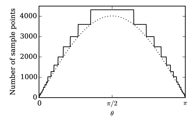
Figure 4.— Number of SymPix grid points per ring as a function of latitude (solid line). The dotted line shows $\alpha_{i}$, i.e., the same quantity for the reduced Gauss-Legendre grid (Reinecke & Seljebotn, 2013).

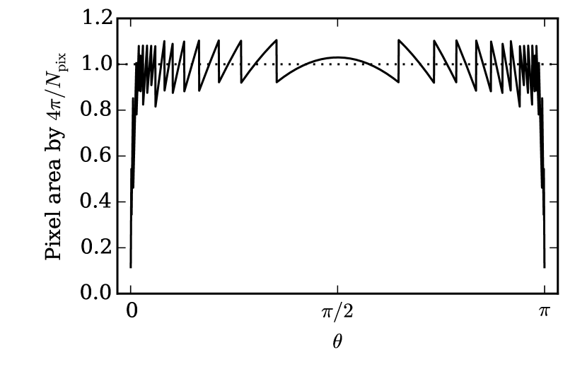
Figure 5.— SymPix pixel area as a function of latitude in units of $4\pi/N_{\text{pix}}$ (solid line). For the HEALPix grid, pixel areas are perfectly uniform (dotted line), while significant over-sampling occurs close to the poles for the SymPix grid.

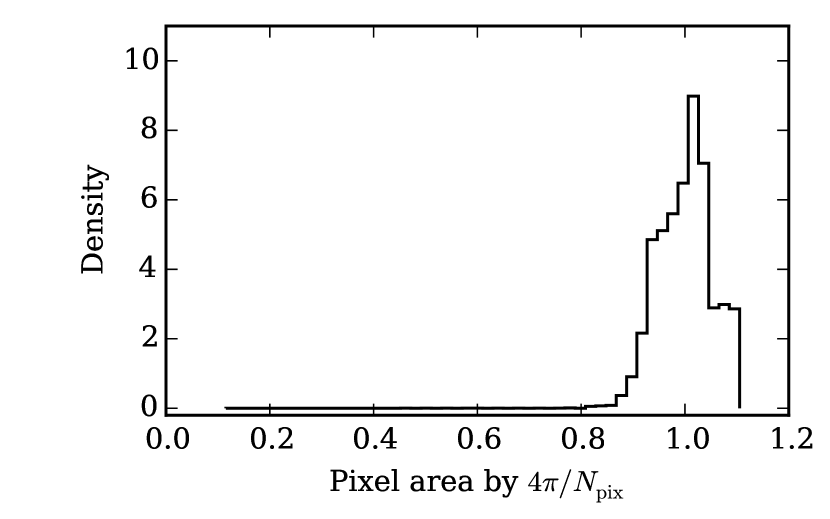
Figure 6.— Histogram of normalized SymPix pixel areas. The tail extending below 0.8 corresponds to polar oversampling, and contains about 0.4% of the total number of pixels for this particular grid setup.

Table 1Comparison of different grids in terms of number of pixels and accuracy of spherical harmonic analysis

$\ell_{\text{max}}$	Grid	Parameter	$N_{\text{pix}}$	$N_{\text{pix}}/N_{\text{pix}}^{\text{HEALPix}}$	Max. error	Mean error	CPU time for SHT (ms)
511	HEALPix	$N_{\text{side}}=256$	786 432	1.00	$2.1\cdot 10^{-2}$	$2.9\cdot 10^{-5}$	160
	SymPix	$\ell_{\text{max}}=511$	390 656	0.50	$7.8\cdot 10^{-3}$	$8.1\cdot 10^{-7}$	67
	Gauss-Legendre	$\ell_{\text{max}}=511$	524 288	0.67	$7.5\cdot 10^{-13}$	$2.8\cdot 10^{-14}$	66
639	HEALPix	$N_{\text{side}}=256$	786 432	1.00	$2.2\cdot 10^{-1}$	$1.3\cdot 10^{-3}$	219
	SymPix	$\ell_{\text{max}}=639$	591 232	0.75	$7.2\cdot 10^{-3}$	$1.1\cdot 10^{-6}$	118
	Gauss-Legendre	$\ell_{\text{max}}=639$	819 200	1.04	$1.2\cdot 10^{-12}$	$3.2\cdot 10^{-14}$	118
767	HEALPix	$N_{\text{side}}=256$	786 432	1.00	$1.6\cdot 10^{0}$	$6.8\cdot 10^{-2}$	287
	SymPix	$\ell_{\text{max}}=767$	838 656	1.07	$4.0\cdot 10^{-2}$	$4.8\cdot 10^{-6}$	188
	Gauss-Legendre	$\ell_{\text{max}}=767$	1 179 648	1.50	$1.0\cdot 10^{-12}$	$3.8\cdot 10^{-14}$	188

Note. — The HEALPix resolution is kept constant at $N_{\text{side}}=256$, while the spherical harmonic bandlimit varies over $\ell_{\text{max}}=\{2.0,2.5,3.0\}N_{\text{side}}$. The SymPix and Gauss-Legendre band-limits are identical to the spherical harmonic band-limit.

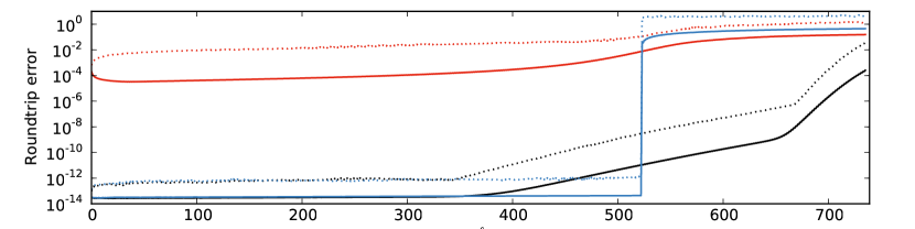
Figure 7.— Spherical harmonic round-trip error as a function of multipole, summarized in terms of maximum (dotted lines) and mean (solid lines) errors, averaged over both harmonic quantum number $m$ and $N_{\textrm{sim}}=100$ simulations. Black lines show results for a SymPix grid with $\ell_{\textrm{max}}=735$ and tile-size $8$; red lines show results for a HEALPix grid with $N_{\text{side}}=256$ and $\ell_{\textrm{max}}=735$; and blue lines show results for a regular Gauss-Legendre grid with $\ell_{\textrm{max}}=628$. All grids have roughly the same number of grid points, $N_{\text{pix}}\approx 780\,000$.

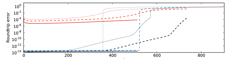
Figure 8.— Error induced by under-sampling (aliasing) as a function of multipole in terms of average errors, averaged over both harmonic quantum number $m$ and $N_{\textrm{sim}}=100$ simulations. The experimental setup is the same as in Figure 7, but the spherical harmonic bandwidth limit varies between $\ell_{\text{max}}=512$ (solid), $\ell_{\text{max}}=735$ (dashed), and $\ell_{\text{max}}=900$ (dotted).

Next, we compare the numerical accuracy of spherical harmonics transforms as implemented on the SymPix, HEALPix and reduced Gauss-Legendre grids. This test is carried out through the following experiment:

1. We draw a fiducial signal $\mathbf{a}=\{a_{\ell m}\}$ in spherical harmonic domain, band-limited by some $\ell_{\text{max}}$. All spherical harmonics coefficients are drawn from the same zero mean and unit variance Gaussian distribution, such that no angular scales dominate the real-space field.

2. We project this signal onto the respective grid sample points by spherical harmonic synthesis.

3. We convert the real-space signal back to harmonic space through spherical harmonic analysis, including multipoles up to $\ell_{\text{max}}$, to recover $\widehat{\mathbf{a}}$.

4. We repeat this procedure $N_{\textrm{sim}}$ times, and summarize the results in terms of the resulting round-trip errors, $e^{(i)}_{\ell m}\equiv\widehat{a}^{(i)}_{\ell m}-a^{(i)}_{\ell m}$.

Before presenting the results, we note that no fundamental band-limit and/or resolution parameter $N_{\text{side}}$ exist for HEALPix for a given angular resolution. For instance, changing the band-limit $\ell_{\text{max}}$ will add/reduce aliasing for all scales. A quantitative head-to-head comparison at a given resolution is therefore difficult, as additional parameter tuning can affect the results. With this caveat in mind, we present in Table 1 results for three different band-limits, $\ell_{\text{max}}=\{2.0,2.5,3.0\}N_{\text{side}}$ with $N_{\text{side}}=256$, quoting both the maximum and mean errors as evaluated over all error coefficients $e^{(i)}_{\ell m}$. Each case includes $N_{\textrm{sim}}=100$ simulations, and the SymPix tile size is fixed at $k=8$.

Starting with the highest bandwidth case, $\ell_{\text{max}}=3N_{\text{side}}$, we first note that the regular Gauss-Legendre grid is the only one grid that achieves overall machine precision, with a mean error of $\mathcal{O}(10^{-14})$ and a maximum error of $\mathcal{O}(10^{-12})$. For comparison, the corresponding mean and maximum SymPix errors are $\mathcal{O}(10^{-6})$ and $\mathcal{O}(10^{-2})$, respectively, while HEALPix achieves $\mathcal{O}(10^{-1})$ and $\mathcal{O}(1)$ for this high bandwidth case. Reducing the bandlimit to $\ell_{\text{max}}=2N_{\text{side}}$ improves the latter by about two orders of magnitude.

However, the statistics listed in Table 1 provide only a very coarse comparison, because the round-trip errors are highly scale dependent. In Figure 7 we therefore plot the error as a function of multipole, $\ell$, choosing the SymPix and HEALPix bandlimits such that the corresponding grids roughly match a HEALPix $N_{\textrm{side}}=256$ grid in terms of total number of sample points. For SymPix, this corresponds to $\ell_{\text{max}}=735$, and for the Gauss-Legendre grid it is $\ell_{\text{max}}=628$.

Starting with the Gauss-Legendre grid (blue lines), we see that the error reaches machine precision up to the bandwidth limit; at higher multipoles no information is carried by the grid. In contrast, the SymPix grid reaches machine precision up to $\ell\approx 0.5\ell_{\text{max}}$, while the error increases more smoothly at higher multipoles. However, even though the high-$\ell$ error increase is smooth, it is still exponential, and the mean and maximum statistics listed in Table 1 are therefore strongly dominated by the small-scale errors. Thus, by virtue of deriving its main geometric grid layout from the Gauss-Legendre grid, we see that the numerical performance of the SymPix grid is excellent on large and intermediate angular scales, and the cost of its superior symmetry properties primarily comes in the form of sub-optimal small-scale residuals. For comparison, the HEALPix errors are roughly constant at $\mathcal{O}(10^{-4})$ to $\mathcal{O}(10^{-2})$, and vary only weakly with angular scale. Note that in all cases the errors can be reduced by iteration techniques, essentially using least squares minimization to find the spherical harmonic signal with least power that projects exactly to the map, and employing the result of spherical harmonic analysis as a preconditioner.

The large errors seen for the Gauss-Legendre grid above $\ell_{\text{max}}$ is due to under-sampling or, equivalently, aliasing. In Figure 8 we study this effect directly by varying the spherical harmonics bandwidth limit between $\ell_{\text{max}}^{\textrm{SH}}=512$, 735 and 900; note, however, that the actual grid resolution parameters are kept fixed at the above values, and the higher resolutions enforced here therefore no longer match the respective grid properties. Considering first the Gauss-Legendre grid with a SHT bandlimit of $\ell_{\text{max}}=512$, we see, as expected, that the errors reach machine precision at all scales. However, for the higher bandlimits, $\ell_{\text{max}}=735$ and 900, both of which are higher than the grid resolution of $\ell_{\text{max}}^{\textrm{grid}}=628$, the errors saturate at a multipole below the grid resolution. To be specific, the critical multipole is $2\ell_{\text{max}}^{\textrm{grid}}-\ell_{\text{max}}^{\textrm{SH}}$, corresponding to the well-known aliasing limit from standard Fourier theory. However, at lower multipoles no aliasing is observed for the Gauss-Legendre grid, which implies that it is fully robust with respect to under-sampling, given a known bandlimit.

In comparison, the corresponding HEALPix errors are non-local, in the sense that increasing the spherical harmonics bandlimit increases the errors at all angular scales: The dotted line ($\ell_{\text{max}}=900$) lies consistently higher than the dashed line ($\ell_{\text{max}}=735$), which in turn lies consistently higher than the solid line ($\ell_{\text{max}}=512$). The HEALPix grid is thus not robust against under-sampling, and it is very important to choose a grid resolution appropriate for the bandwidth of the signal under consideration, which in several applications may imply over-sampling the signal.

The SymPix grid performance lies, as expected, between those of Gauss-Legendre and HEALPix. On large angular scales, it achieves numerical precision, while on small scales the aliasing increases exponentially with multipole, and eventually reaches similar levels as HEALPix.

3.3. Computational speed of SHTs

Before ending this section, we compare the performance of the SymPix, HEALPix and Gauss-Legendre grids in terms of computational speed. The rightmost column in Table 1 lists the CPU time for each of the cases considered above in units of wall-clock milli-seconds, while Figure 9 presents a head-to-head comparison of the SymPix and HEALPix grid performance as a function of $N_{\text{pix}}$. All benchmarks were performed using libsharp on a single Intel Core i7 Q840 at 1.87 GHz (SSE2); for full details including CPU times in absolute numbers, we refer the interested reader to Reinecke & Seljebotn (2013).

Overall, SymPix perform similarly to the Gauss-Legendre grid, and both execute about 30 % faster than HEALPix. This latter difference may be explained by the fact that the HEALPix grid points form a zig-zag pattern in which every other ring is longitudinally shifted by half a pixel width. This implies a grid point organization that comprise about 30 % more rings than Gauss-Legendre and SymPix grids, which exhibit more regular longitudinal pixel organizations. This is relevant, because the computational complexity of SHTs scales as

$$C_{\text{SHT}} =\mathcal{O}(N_{\text{ring}}\ell_{\text{max}}^{2})+\mathcal{O}(N_{\text{pix}}\log\frac{N_{\text{pix}}}{N_{\text{ring}}})$$ (6)

$$=\mathcal{O}(\ell_{\text{max}}^{3})+\mathcal{O}(\ell_{\text{max}}^{2}\log\ell_{\text{max}}).$$

The first term represents the cost of computing the associated Legendre polynomials for each ring, and dominates the second term, which accounts for evaluating Fast Fourier Transforms (FFTs) along each ring. Thus, the number of grid points per ring is not critical for the overall speed of SHTs, while the total number of rings is.

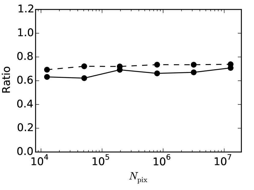
Figure 9.— Comparison between spherical harmonic transforms cost as performed with SymPix and HEALPix as a function of $N_{\text{pix}}$, plotted in terms of their ratio (black solid line). The dashed line shows the ratio between the number of grid point rings.

In addition, SymPix grids have by construction rings with pixel numbers that are only products of $2$, $3$ and/or $5$, which ensures efficient Fast Fourier Transforms (FFTs). In contrast, many HEALPix rings have pixel numbers that includes large primes, and therefore the Bluestein algorithm must be employed for these. This effect is more important for lower resolution grids, for which the cost of FFTs is relatively higher.

4. Applications

We now turn our attention to practical applications, and in particular to the construction of efficient preconditioners. Before doing that, however, we consider a simpler application, namely real-space convolution, in order to build up intuition regarding the relevant operations. We emphasize that the purpose of this preliminary discussion is not to provide a real-world alternative to spherical harmonic transforms, or the methods presented by Elsner & Wandelt (2011) and Sutter et al. (2012) for such convolutions, but simply to quantify the computational efficiency of the SymPix grid on a simple and intuitive application.

4.1. Spherical convolution

The convolution of a spherical image $f$ with a kernel $b$ is given by the spherical surface integral

$$g(\hat{n})=\int_{4\pi}b(\hat{n},\hat{m})f(\hat{m})d\Omega_{\hat{m}}.$$ (7)

In our case we assume an azimuthally symmetric kernel, and $b(\hat{n},\hat{m})$ therefore depends only on the distance between $\hat{n}$ and $\hat{m}$, such that

$$g(\hat{n})=\int_{4\pi}b(\hat{n}\cdot\hat{m})f(\hat{m})d\Omega_{\hat{m}}.$$ (8)

This integral is most commonly performed in spherical harmonic domain, turning full-sky convolution into coefficient-wise multiplication with a corresponding transfer function, $b_{\ell}$, which is given by the Legendre transform of $b(\hat{n}\cdot\hat{m})$. These computations are dominated by the spherical harmonic transforms, and therefore have a computational scaling of $\mathcal{O}(N_{\text{pix}}^{3/2})=\mathcal{O}(\ell_{\text{max}}^{3})$.

If $b$ is spatially narrow compared to the required pixelization, as is usually the case, one could instead consider the pixel-domain convolution by evaluating

$$g(\hat{n}_{i})=\sum_{j=1}^{N_{\text{pix}}}b(\hat{n}_{i}\cdot\hat{n}_{j})f(\hat{n}_{j}),$$ (9)

where the convolution kernel reads

$$b(x)=\sum_{\ell=0}^{\ell_{\text{max}}}\frac{2\ell+1}{4\pi}b_{\ell}P_{\ell}(x).$$ (10)

One would then make the approximation that $b(\hat{n}_{i}\cdot\hat{n}_{j})=0$ whenever sample points $i$ and $j$ are more than $k$ sample point distances apart, as discussed in Section 1.

For HEALPix, almost all sample point distances are different, and $b$ must therefore be evaluated $\mathcal{O}(N_{\text{pix}}\,k^{2})$ times. The computational complexity of pixel-domain convolution on the HEALPix grid therefore scales as $\mathcal{O}(N_{\text{pix}}\,k^{2}\,\ell_{\text{max}})=\mathcal{O}(k^{2}\,\ell_{\text{max}}^{3})$, which is clearly inferior to the harmonic approach both in terms of speed and accuracy. With SymPix, however, the large number of symmetries allows us to reduce the computational complexity to $\mathcal{O}(k^{2}\,N_{\text{pix}}+\sqrt{N_{\text{pix}}}\,\ell_{\text{max}})=\mathcal{O}(k^{2}\,N_{\text{pix}})$: One simply needs to choose a tile size $k$ such that only sample point pairs within a tile and between neighbouring tiles must be considered. Then for, each band of $k$ rings, $b(\hat{n}\cdot\hat{m})$ only needs to be evaluated for the first few tiles of the band, as other distances within the same band will be identical within the remainder of the band.

The speed-up for evaluating all necessary $b(\hat{n}\cdot\hat{m})$, when approximating $b(\hat{n}\cdot\hat{m})=0$ whenever $\hat{n}$ and $\hat{m}$ are not in neighbouring tiles, are given in Table 2. In addition to scaling better than the $\mathcal{O}(N_{\text{pix}}^{3/2})$ spherical harmonic transforms, this approach should also be easier to parallelize and implement efficiently on a GPU.

Table 2CPU time and theoretical speed-up for evaluating $b(\hat{n}\cdot\hat{m})$

	CPU time	Speed-up
$\ell_{\text{max}}$	[sec]	[factor]
3000	9.80	732
1500	3.60	335
0750	1.40	149
0375	0.74	070
0188	0.50	026
0100	0.31	014

Note. — We have approximated $b(\hat{n}\cdot\hat{m})=0$ whenever $\hat{n}$ and $\hat{m}$ are not in neighbouring tiles. The third column shows the number of non-zero $b(\hat{n}\cdot\hat{m})$, which scales as $O(k^{2}N_{\text{pix}})$, divided by the number of elements we had to compute when making use of the SymPix symmetries, which scales as $O(k^{2}\sqrt{N_{\text{pix}}})$. In this example we have chosen $k=8$.

Note that yet another method for spherical convolution with a symmetric kernel has been implemented in the ARKCoS code (Elsner & Wandelt, 2011; Sutter et al., 2012), with a computational scaling of $\mathcal{O}(k\,\ell_{\text{max}}^{2}\,\text{log}\,\ell_{\text{max}})=\mathcal{O}(k\,N_{\text{pix}}\,\log\,N_{\text{pix}})$. Whether a SymPix-based convolution would improve relative to their work for relevant resolution parameters and accuracy requirements remains to be explored.

4.2. Preconditioner construction for linear systems

Finally, we are in the position to discuss the application of the SymPix grid to our main usecase, namely for solving linear systems involving rotationally invariant operators in pixel domain, either through multi-grid methods or to construct efficient preconditioners. The simplest example of such a system is

$$\mathbf{Y}\mathbf{B}\mathbf{Y}^{T}\mathbf{x}=\mathbf{b},$$ (11)

where $\mathbf{Y}$, as usual, is the matrix corresponding to spherical harmonic synthesis and $\mathbf{B}$ is a diagonal matrix in spherical harmonic domain, $B_{\ell m,\ell^{\prime}m^{\prime}}=b_{\ell}\delta_{\ell,\ell^{\prime}}\delta_{mm^{\prime}}$. The product $\mathbf{Y}\mathbf{B}\mathbf{Y}^{T}$ is a pixel domain operator with strong spatial couplings within the correlation length implied by $b$. Of course, this particular system could have been trivially solved by converting to spherical harmonic domain, which would diagonalize the coefficient matrix. However, if there are more terms in the operator, this is no longer possible, and iterative solvers like Conjugate Gradients or multi-level algorithms are needed. In these cases SymPix is useful to construct preconditioners or smoothers.

Our own main interest lies in drawing constrained Gaussian realizations of the CMB sky by using a multi-level solver (Seljebotn et al., 2014). This may performed by solving the following linear system (Jewell et al., 2004; Wandelt et al., 2004; Eriksen et al., 2004),

$$\mathbf{Y}_{1}(\mathbf{D}+\mathbf{B}\mathbf{Y}_{\text{obs}}\mathbf{N}^{-1}\mathbf{Y}_{\text{obs}}^{T}\mathbf{B})\mathbf{Y}_{1}^{T}\mathbf{x}=\mathbf{r},$$ (12)

where $\mathbf{D}$ and $\mathbf{B}$ are diagonal matrices in spherical harmonic domain, characterized by transfer functions $d_{\ell}$ and $b_{\ell}$, $\mathbf{N}^{-1}$ is a diagonal (inverse noise covariance) matrix in pixel domain, pixelized on some external grid $\theta_{i}$, and $\mathbf{r}$ is a stochastic term that depends on the data set in question.

Two different spherical grids are involved in system. First, the outermost spherical harmonics transform, $\mathbf{Y}_{1}$, denotes synthesis to a grid of our own choosing. We will use a SymPix grid of resolution $\ell_{\text{max}}$ for this operator in the following. The inner transform, $\mathbf{Y}_{\text{obs}}$, is determined by some external experiment, and is thus not flexible. Here we will assume that this operator is defined on a full-sky HEALPix grid of $N_{\text{side}}=2048$, typical for the CMB maps published by the Planck experiment (Planck Collaboration, 2015).

Of course, from the viewpoint of the overall linear system, the details of any individual operator is irrelevant, and the only crucial point is that the combined operator remains the same. In order to speed up the calculations through use of symmetries, we therefore substitute the inner-most HEALPix based noise covariance matrix product with a corresponding SymPix based product,

$$\mathbf{Y}_{\text{obs}}\mathbf{N}^{-1}\mathbf{Y}_{\text{obs}}^{T}=\mathbf{Y}_{2}\mathbf{N}_{2}^{-1}\mathbf{Y}_{2}^{T}$$ (13)

where $\mathbf{Y}_{2}$ denotes an auxiliary SymPix grid; note that this does not need to be the same as $\mathbf{Y}_{1}$, but its resolution can be adjusted to trade numerical precision for computational speed. As shown by Seljebotn et al. (2014), Equation 13 holds true if $\mathbf{N}_{2}$ is constructed from

$$\mathbf{\theta}_{2}=\mathbf{W}_{2}\mathbf{Y}_{2}\mathbf{Y}_{\text{obs}}^{T}\mathbf{\theta},$$ (14)

in the same way as $\mathbf{N}$ is constructed from $\theta$. In this latter expression, $\mathbf{W}_{2}$ is a diagonal matrix containing the quadrature weights used in the spherical harmonic analysis of the target grid, while $\mathbf{Y}_{\text{obs}}^{T}$ lacks the ring weights one normally uses in spherical harmonic analysis. Note that this operation is in fact the opposite procedure compared to naive resampling, which would be written $\mathbf{Y}_{2}\mathbf{Y}_{\text{obs}}^{T}\mathbf{W}_{\text{obs}}$ in our notation. For full details, we refer the interested reader to Seljebotn et al. (2014).

Table 3CPU time for constructing preconditioner

	HEALPix	SymPix
$\ell_{\text{max}}$	(CPU min)	(CPU min)	Speed-up
Evalution of $\widehat{\mathbf{B}}^{T}\mathbf{N}^{-1}\widehat{\mathbf{B}}$
3000	727	5.400	00130
1500	509	1.400	00360
750	340	0.370	00920
375	230	0.110	02 100
188	452	0.035	13 000
0100	363	0.027	13 000
Sum	2 6210	7.300	00360
Evalution of $\widehat{\mathbf{D}}$
3000	00085.000	3.30	00026
1500	00015.000	0.83	00018
750	0002.40	0.22	00011
375	0000.36	0.07	00005
188	0000.05	0.02	00003
0100	0000.01	0.01	00001
Sum	000103.0000	4.50	00023

Note. — The top section lists the CPU time for preconditioner calculations that depend only on data geometry (mask, beam, noise characterization), while the bottom section lists the corresponding CPU time for calculations that depend on $d_{\ell}$, which in CMB applications typically corresponds to an angular power spectrum, $C_{\ell}$. The second column is copied directly from Seljebotn et al. (2014), and shows results using HEALPix for all calculations. The third row shows similar results using SymPix, while the fourth column shows the ratio between the two.

The precision of Equation 13 depends on the relative bandlimit of $\mathbf{Y}_{1}$, $\mathbf{Y}_{2}$ and $\mathbf{Y}_{\text{obs}}$. For instance, choosing $\ell_{\text{max}}$ for $\mathbf{Y}_{2}$ and $\mathbf{Y}_{\text{obs}}$ to be twice that of $\mathbf{Y}_{1}$ yields a numerical precision of $\mathcal{O}(10^{-10})$. Increasing these to four times that of $\mathbf{Y}_{1}$ results in an accuracy of $\mathcal{O}(10^{-14})$, whereas reducing it to only one, such that $\mathbf{Y}_{1}=\mathbf{Y}_{2}$, gives an accuracy of $\mathcal{O}(10^{-2})$. Even the latter may be acceptable for preconditioning purposes.

In order to derive an approximation to the full coefficient matrix defined by Equation 12, we first re-write the system as

$$\widehat{\mathbf{D}}+\widehat{\mathbf{B}}^{T}\mathbf{N}_{2}^{-1}\widehat{\mathbf{B}}\mathbf{x}=\mathbf{r},$$ (15)

where

$$\widehat{\mathbf{D}}=\mathbf{Y}_{1}\mathbf{D}\mathbf{Y}_{1}^{T}\quad\text{and}\quad\widehat{\mathbf{B}}=\mathbf{Y}_{2}\mathbf{B}\mathbf{Y}_{1}^{T}.$$ (16)

We now introduce the approximation that $\widehat{D}_{ij}=0$ and $\widehat{B}_{ij}=0$ whenever two sample points $i$ and $j$ are not in the same or neighbouring tiles, as per the SymPix organization. The non-zero elements (i.e., the “local” part) of $\widehat{\mathbf{D}}$ and $\widehat{\mathbf{B}}$ are evaluated by Equation 10, at a cost of $\mathcal{O}(\ell_{\text{max}})$ operations per matrix element. However, as discussed in Section 4.1, evaluating all required elements for a SymPix grid scales as $\mathcal{O}(k^{2}\,\sqrt{N_{\text{pix}}})$, as opposed to $\mathcal{O}(k^{2}\,N_{\text{pix}})$ for less symmetric grids.

These calculations constitute essential components of the pre-computation step of the multi-grid solver presented by Seljebotn et al. (2014). In that paper, all evaluations were performed with the HEALPix grid, with a computational scaling of $\mathcal{O}(\ell_{\text{max}}k^{2}N_{\text{pix}})$ as discussed above. Their Table 2 summarizes the resulting computational costs in units of CPU minutes. Here we repeat those calculations adopting exactly the same overall parameters, facilitating a one-to-one comparison, but we employ SymPix for intermediate calculations instead of HEALPix. The results are summarized in Table 3, in which the second column is copied directly from Seljebotn et al. (2014), and the third column shows the new SymPix results. The fourth column shows the ratio between the two.

Clearly, the net gains achieved by the SymPix grid varies with resolution. For the high resolution levels the speed-up is driven by symmetries drastically reducing the time taken to evaluate $\widehat{\mathbf{B}}$. The theoretical speed-up of 732 times for evaluating $\widehat{\mathbf{B}}$ at $\ell_{\text{max}}=3000$, found in Table 2, is reduced to 130 and 26 for $\widehat{\mathbf{B}}^{T}\mathbf{N}^{-1}\widehat{\mathbf{B}}$ and $\widehat{\mathbf{D}}$, respectively. This is due to work that was previously unimportant now dominating the computation. At lower resolutions the speed-up is almost entirely due to being able to use the operator resampling given in Equation (13). This degradation procedure is not possible when using the HEALPix grid, and so our previous code had to use a resolution of $N_{\text{side}}=2048$ along columns and level resolution along rows.

Overall, the SymPix grid reduces what used to be over-night jobs to essentially interactive tasks.

5. Conclusion

We have presented SymPix, a novel spherical grid for efficient sampling of rotationally invariant operators. This grid derives many of its properties from the Gauss-Legendre grid, ensuring overall excellent spherical harmonics transform performance. The main difference between the two grids is that SymPix sacrifices proper Nyquist sampling in the longitudinal direction in order to increase pixel symmetries, such that all grid pair distances repeat perfectly along constant-latitude rings. This decreases the computational scaling of evaluating rotationally invariant operators from $\mathcal{O}(N_{\text{pix}})$ to $\mathcal{O}(\sqrt{N_{\text{pix}}})$.

The intended primary application of the SymPix grid is efficient construction of preconditioners (or smoothers) for iterative linear solvers. In this paper we considered the specific example of drawing constrained Gaussian realizations using a multi-grid solver, which is an important problem in current CMB analysis. Comparing with previous state-of-the-art results based on the HEALPix grid (Seljebotn et al., 2014), we achieve average speed-ups of 360 and 23 for the two most important pre-computation steps when using SymPix for internal calculations.

However, we emphasize that SymPix is a special-purpose grid designed for precisely such tasks; it is not intended to provide a general purpose spherical pixelization that is suitable for, say, map making. HEALPix is clearly preferred for such purposes due to its uniform pixel areas, regular pixel window and hierarchical pixel structure. Likewise, if machine precision spherical harmonics transforms are required, the Gauss-Legendre grid is the obvious choice. However, for those particular applications that can benefit from efficient pixel space sampling of linear operators, such as ours, SymPix holds a clear edge over existing alternatives.

Appendix A Code

The SymPix code has been developed as part of the Commmander project, and does not yet have its own library. For the benefit of the reader we have however copied the source files relevant to this paper to its own repository at http://github.com/dagss/sympix. Please consult the accompanying README file for further details. This repository will be updated if the code does eventually develop into a stand-alone package.

The SHTs are all done using libsharp (Reinecke & Seljebotn, 2013), at the time of writing available at http://sourceforge.net/projects/libsharp/. We then construct the grid geometry in our Python code and feed it to libsharp. In the future we may port our Python code to C and make it available directly in libsharp.

References

- Cormen et al. (1989) Cormen, T. H., Leiserson, C. E., Rivest, R. L. 1989, Introduction to Algorithms (MIT Press)
- Doroshkevich et al. (2005) Doroshkevich, A. G., Naselsky, P. D., Verkhodanov, O. V., et al. 2005, International Journal of Modern Physics D, 14, 275
- Elsner & Wandelt (2011) Elsner, F., & Wandelt, B. D. 2011, A&A, 532, A35
- Eriksen et al. (2004) Eriksen, H. K., O’Dwyer, I. J., Jewell, J., Wandelt, B. D., Larson, D. L., Górski, K. M., Levin, S., Banday, A. J., Lilje, P. B, ApJS, 155, 227
- Górski et al. (2005) Górski, K. M., Hivon, E., Banday, A. J., Wandelt, B. D., Hansen, F. K., Reinecke, M., & Bartelmann, M. 2005 ApJ, 622, 2
- Jewell et al. (2004) Jewell, J., Levin, S., & Anderson, C. H. 2004, ApJ, 609, 1
- Planck Collaboration (2015) Planck Collaboration 2015, A&A, submitted, [arXiv:1502.01582]
- Prézeau & Reinecke (2010) Prézeau, G., & Reinecke, M. 2010, ApJS, 190, 267
- Reinecke (2011) Reinecke, M. 2011, A&A, 526, A108
- Reinecke & Seljebotn (2013) Reinecke, M., & Seljebotn, D. S. 2013, A&A, 554, A112
- Seljebotn (2012) Seljebotn, D. S. 2012, ApJS, 199, 5
- Seljebotn et al. (2014) Seljebotn, D. S., Mardal, K.-A., Jewell, J. B., Eriksen, H. K., & Bull, P. 2014, ApJS, 210, 24
- Sutter et al. (2012) Sutter, P., Wandelt, B. D., & Elsner, F. 2012, Proceedings of ”Big Bang, Big Data, Big Computers” (Big3). September 19-21, 2012.
- Wandelt et al. (2004) Wandelt, B. D., Larson, D. L., & Lakshminarayanan, A. 2004, Phys. Rev. D, 70, 083511