Fundamental differences between glassy dynamics in two and three dimensions

Abstract

The two-dimensional freezing transition is very different from its three-dimensional counterpart. In contrast, the glass transition is usually assumed to have similar characteristics in two and three dimensions. Using computer simulations we show that glassy dynamics in supercooled two- and three-dimensional fluids are fundamentally different. Specifically, transient localization of particles upon approaching the glass transition is absent in two dimensions, whereas it is very pronounced in three dimensions. Moreover, the temperature dependence of the relaxation time of orientational correlations is decoupled from that of the translational relaxation time in two dimensions but not in three dimensions. Lastly, the relationships between the characteristic size of dynamically heterogeneous regions and the relaxation time are very different in two and three dimensions. These results strongly suggest that the glass transition in two dimensions is different than in three dimensions.

I Introduction

In two-dimensional (2D) solids, thermal fluctuations destroy crystalline order, displacement correlations increase logarithmically, and density correlations decay according to power laws Strandburg1988 ; Mermin1968 . However, there can be long-range bond-orientational order in 2D Mermin1968 . The transition from the 2D fluid phase to the solid phase can occur in two steps with an intermediate phase characterized by an exponential decay of the density correlations and a power-law decay of the bond-orientational correlations Strandburg1988 ; Bernard2011 . In contrast, in three-dimensional (3D) solids fluctuations do not destroy crystalline order Peierls1935 , and long-range translational and rotational order emerge together at the freezing transition.

Despite these differences between two- and three-dimensional ordered solids, the formation of an amorphous solid upon supercooling a fluid, i.e. the glass transition, is generally assumed to have similar characteristics in 2D and 3D Harrowell2006 . This assumption is reflected in the trivial dimensional dependence of most glass transition theories Berthier2011 .

We show that structural relaxation of supercooled fluids in two dimensions is different than in three dimensions. While we find the transient localization often associated with glassy dynamics in three dimensions, we do not find any transient localization in two dimensions if we simulated systems large enough to remove any finite size effects. Furthermore, the temperature dependence of the bond-orientational correlation time is decoupled from that of the translational relaxation time time in two dimensions, but these relaxation times have very similar temperature dependence in three dimensions. Along with these differences in structural relaxation, we also find that the characteristic size of regions of correlated mobility, dynamic heterogeneities, increases faster with the structural relaxation time in two dimensions than in three dimensions, and these regions are more ramified in two dimensions than three dimensions. Lastly, we show that the structural relaxation and heterogeneous dynamics depends on the underlying dynamics in two dimensions.

II Results

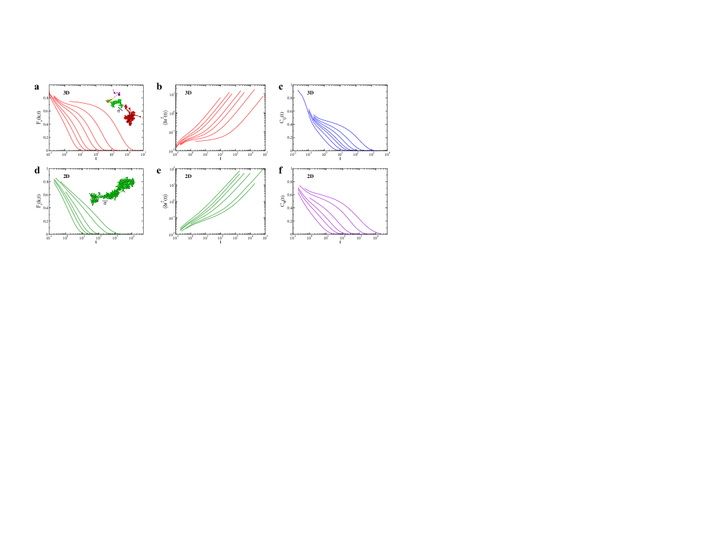
Figure 1: Structural relaxation in two and three dimensions. a, The self-intermediate scattering function $F_{s}(k;t)$ for the 3D glass-former for $T=1.0$, 0.8, 0.7, 0.6, 0.55, 0.5, and 0.45 listed from left to right. The mode-coupling temperature $T_{c}^{3D}\approx 0.435$. The inset shows a trajectory plot of one small particle at $T=0.45$ where the color of the trajectory plot changes when the particle moves more than one large particle diameter $\sigma$ (length of the black line) over a time of $0.1\tau_{\alpha}$. b, The mean square displacement $\left<\delta r^{2}(t)\right>$ for the 3D system showing the same temperatures as in (a). c, The bond-orientational correlation function $C_{Q}(t)$ for the 3D glass-former showing the same temperatures as in (a). d, The self-intermediate scattering function $F_{s}(k;t)$ for the 2D glass-former for $T=1.0$, 0.8, 0.7, 0.6, 0.5, and 0.45 listed from left to right. The inset shows a trajectory plot of a small particle, and no sudden jumps are observed. e, The mean square displacement $\left<\delta r^{2}(t)\right>$ for the 2D system showing the same temperatures as in (d). f, The bond-orientational correlation function $C_{\Psi}(t)$ for the 2D glass-former showing the same temperatures as in (d).

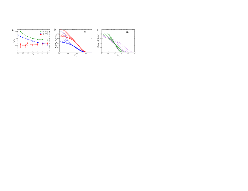
Figure 2: Bond angle and translational relaxation times. a, The ratio of the relaxation time for the bond-orientational correlation functions $\tau_{\theta}$ and the self-intermediate scattering function $\tau_{\alpha}$ for the 2D system (circles) and the 3D system (squares). The ratio $\tau_{\theta}/\tau_{\alpha}$ for the 3D system is approximately constant and equal to 0.1-0.2 over the entire range of temperatures. The green circles are for Newtonian dynamics (ND) and the blue circles are results for Brownian dynamics (BD). b, The self-intermediate scattering function $F_{s}(k;t)$ (red solid lines) and the bond-angle time correlation function $C_{Q}(t)$ (blue lines) rescaled by $\tau_{\alpha}$ for the 3D system. c, The self-intermediate scattering function $F_{s}(k;t)$ (green solid lines) and the bond-angle time correlation function $C_{\Psi}(t)$ (violet dashed lines) rescaled by $\tau_{\alpha}$ for the 2D system.

Structural relaxation. To demonstrate the differences between glassy dynamics in two and three dimensions, we focus on two closely related glass-forming fluids: the 3D 80:20 binary Lennard-Jones system introduced by Kob and Andersen Kob1994 , and its 2D variant that has the same interaction potentials but a 65:35 composition to avoid crystallization Bruning2009 . To simulate the relaxation in these systems we used the standard Newtonian dynamics AT . We also simulated the 2D system using Brownian dynamics AT and we comment on the differences between these two dynamics. See Methods for the simulation details and the reduced units used to present the results. We examined three other 2D glass formers and one additional 3D glass former (see Methods for details of the systems) and present results, which are qualitatively the same as the results for the KA system, in the supplemental material.

In 3D, the dominant feature in the dynamics of deeply supercooled glass-forming fluids is transient localization of individual particles Berthier2011 , which is illustrated in the inset to Fig. 1a. The transient localization results in characteristic plateaus of the self-intermediate scattering function, $F_{s}(k;t)=N^{-1}\left<\sum_{n}e^{i\mathbf{k}\cdot[\mathbf{r}_{n}(t)-\mathbf{r}_{n}(0)]}\right>$ (k=7.2 in 3D and 6.28 in 2D), shown in Fig. 1(a), and the mean-square displacement, $\left<\delta r^{2}(t)\right>=N^{-1}\left<\sum_{n}[\mathbf{r}_{n}(t)-\mathbf{r}_{n}(0)]^{2}\right>$, shown in Fig. 1b. The plateaus extend to longer and longer times upon approaching the glass transition. Similar plateaus are observed in the collective scattering function, $F(k;t)=N^{-1}\left<\sum_{n,m}e^{i\mathbf{k}\cdot[\mathbf{r}_{n}(t)-\mathbf{r}_{m}(0)]}\right>$, which describes relaxation of the density field (not shown), and in the correlation function quantifying bond-orientational correlations in 3D, $C_{Q}(t)$, shown in Fig. 1c (see Methods for the definition of $C_{Q}$). Qualitatively similar slowing down of the translational and bond-orientational relaxation in 3D glass forming fluids is analogous to the simultaneous appearance of translational and rotational long range order in 3D crystalline solids.

The transient localization observed in 3D glassy dynamics is absent in 2D, as showed in the inset to Fig. 1d. Correspondingly, there is no intermediate time plateau in the self-intermediate scattering function in 2D, Fig. 1d. The final decay of $F_{s}(k;t)$, which in 3D is well described by a stretched exponential, is replaced by a very slow decay in 2D. The intermediate time plateau in the mean-square displacement observed in 3D is replaced by an extended sub-diffusive regime in 2D, Fig. 1e. However, an intermediate time plateau is observed in the correlation function quantifying bond-orientational correlations in 2D, $C_{\Psi}(t)$, Fig. 1f (see Methods for the definition of $C_{\Psi}$). Shown in Supplemental Figure 1a-c are $F_{s}(k;t)$ and $C_{\Psi}(t)$ for three additional 2D glass formers and they behave similarly. Qualitatively different behavior of the translational and bond-orientational relaxation in 2D glass forming fluids is analogous to the absence of the translational and the presence of the bond-orientational long-range order in 2D solids Strandburg1988 .

To quantify decoupling between translational and bond-orientational relaxation we compare the temperature dependence of the relaxation times characterizing $F_{s}(k;t)$ and $C_{(Q,\Psi)}(t)$, where $Q$ and $\Psi$ refer to 3D and 2D correlation functions. We define the translational relaxation time $\tau_{\alpha}$ through the relation $F_{s}(k;\tau_{\alpha})=e^{-1}$ and the bond-orientational relaxation time $\tau_{\theta}$ through $C_{(Q,\Psi)}(\tau_{\theta})=e^{-1}$. At the highest temperatures the ratio $\tau_{\theta}/\tau_{\alpha}$ is less than one for both the 3D and the 2D glass-former, Fig. 2a. However, this ratio stays approximately constant with decreasing temperature for the 3D glass-former, but grows monotonically for the 2D glass-former. In Supplemental Figure 1d we show this ratio for the other 2D glass formers and show that the decoupling is a general feature of 2D glassy dynamics. In addition, in Figs. 2b,c we show that the final translational and orientational relaxation satisfies the time-temperature superposition in 3D but not in 2D, and we show corresponding figures for an additional glass former in 2D and 3D in Supplemental Figure 2. Fig. 2c clearly demonstrates the decoupling of the temperature dependence of the translational and bond-orientational relaxation times in 2D.

Dynamic heterogeneities. The non-exponential decay of $F_{s}(k;t)$ is frequently attributed to the emergence of domains, referred to as dynamic heterogeneities, in which the relaxation is spatially correlated and significantly different (faster or slower) than the average relaxation. While we find non-exponential decay in $F_{s}(k;t)$ for 3D and 2D glass-formers, the nature of the decay is very different and this difference is mirrored by differences in the heterogeneous dynamics.

Shown in Figs. 3a-d are displacement maps showing the center of a four million particle simulation in 2D at $T=0.45$. The maps are created by coloring the particles, whose position is shown on $t=0$, according to the magnitude of their displacements $|\mathbf{r}_{n}(t)-\mathbf{r}_{n}(0)|$ at a time $t$. The red particles have moved a distance equal to or greater than the diameter of a larger particle. There are large domains of particles that have moved less than a particle diameter even at $t=10\,000$.

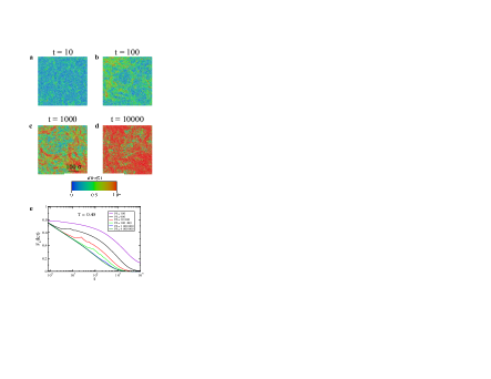
Figure 3: Dynamic heterogeneities. a-d, Displacement maps of the center of a system of 4 million particles that show the position of the particles at $t=0$ colored by the displacement of the particle at a later time $t$ for $T=0.45$. There are approximately $250\,000$ particles in each map. The scale bar in d corresponds to 100 larger particle diameters. e, The self-intermediate scattering function $F_{s}(k;t)$ calculated for systems of 100 to 4 million particles. There are clear finite size effects for less than one million particles.

Considering the large dynamically heterogeneous regions in Figs. 3a-d, it is unsurprising that we also find large finite size effects. Shown in Fig. 3e is $F_{s}(k;t)$ calculated for different size systems at the same temperature as shown in Figs. 3a-d. A plateau reminiscent of the plateau in 3D systems is present for the smaller systems but gradually disappears with increasing system size. Similar finite size effects are also evident in the mean square displacement, Supplemental Figure 3a, and the inherent structure dynamics, Supplemental Figure 3b.

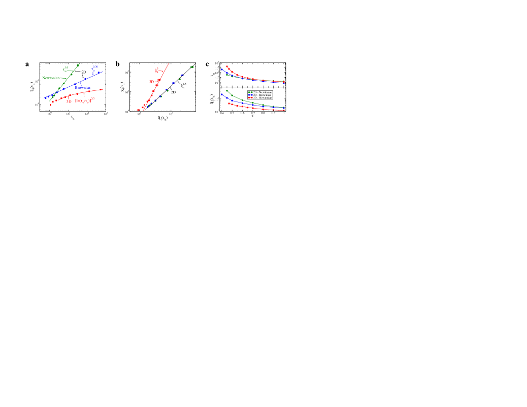
Figure 4: Properties of dynamic heterogeneities. a, The dynamic correlation length $\xi_{4}(\tau_{\alpha})$ versus the translational relaxation time $\tau_{\alpha}$. The circles are the results for the 2D system where the underlying dynamics is Newtonian (green) and Brownian (blue). The lines are fits to a power law $\xi_{4}(\tau_{\alpha})=a\tau_{\alpha}^{\beta}$. The red squares are results for the 3D system where the underlying dynamics is Newtonian. The red line is a fit to $\xi_{4}(\tau_{\alpha})=b[\ln(\tau_{\alpha}/\tau_{o})]^{2/3}$. b, The dynamic susceptibility $\chi_{4}(\tau_{\alpha})$ versus the dynamic correlation length $\xi_{4}(\tau_{\alpha})$ for the 2D system where the underlying dynamics are Newtonian (green circles) and Brownian (blue circles). The red squares are results for the 3D system. The lines are fits to the power laws $\chi_{4}(\tau_{\alpha})\sim\xi_{4}(\tau_{\alpha})^{3}$ in 3D and $\chi_{4}(\tau_{\alpha})\sim\xi_{4}(\tau_{\alpha})^{1.5}$ in 2D. c, The relaxation time $\tau_{\alpha}$ and the dynamic correlation length $\xi_{4}(\tau_{\alpha})$ where the underlying dynamics are Newtonian (green) and Brownian (blue) for the 2D system, and Newtonian for the 3D system (red).

To quantify dynamic heterogeneity shown in Fig. 3a-d we use a four-point structure factor $S_{4}(q;t)$ Flenner2014 constructed from overlap functions $w_{n}(a;t)=\Theta(a-|\mathbf{r}_{n}(t)-\mathbf{r}_{n}(0)|)$, where $\Theta(\cdot)$ is Heaviside’s step function. The parameter $a$ is chosen such that $N^{-1}\left<\sum_{n}w_{n}(a;\tau_{\alpha})\right>\approx F_{s}(k;\tau_{\alpha})$, which results in $a=0.25$ in 3D and $a=0.22$ in 2D. To characterize the slow domains we calculate $S_{4}(q;t)=N^{-1}\left<\sum_{n}\sum_{m}w_{n}(a;t)w_{m}(a;t)e^{i\mathbf{q}\cdot(\mathbf{r}_{n}(0)-\mathbf{r}_{m}(0))}\right>$ (note that $w_{n}(a;t)$ restricts the sums over the particles that moved less than $a$ over a time $t$). The characteristic size of dynamically heterogeneous regions is quantified through the dynamic correlation length $\xi_{4}(t)$, which is determined from fitting $S_{4}(q;t)$ for small $q$ to the Ornstein-Zernicke form $\chi_{4}(t)/\{1+[q\xi_{4}(t)]^{2}\}$. Here $\chi_{4}(t)$ is the dynamic susceptibility, which characterizes the overall strength of the dynamic heterogeneity.

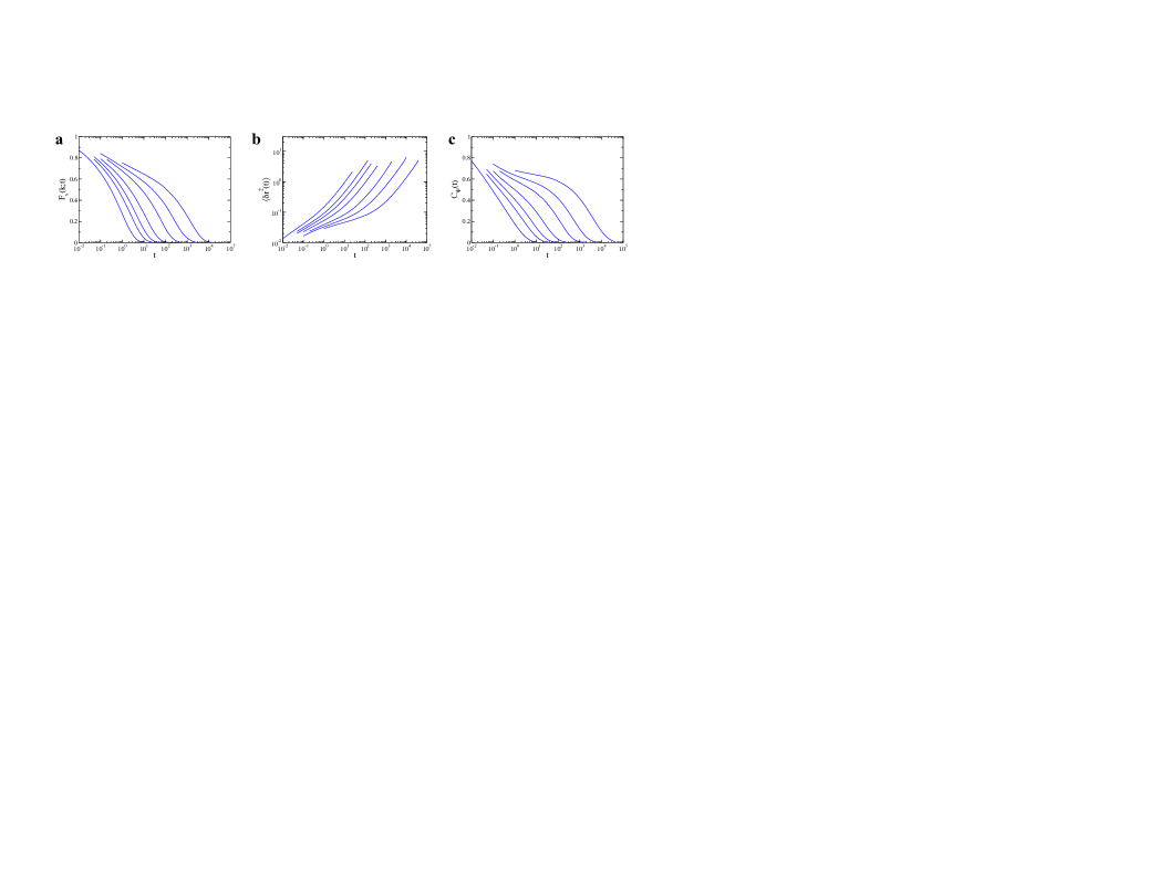
Figure 5: Structural relaxation in two dimensions with Brownian dynamics. a, The self-intermediate scattering function $F_{s}(k;t)$ for $T=1.0$, 0.8, 0.7, 0.6, 0.5, 0.45 and 0.4 listed from left to right. b, The mean square displacement $\left<\delta r^{2}(t)\right>$ showing the same temperatures as in (a). c, The bond angle time correlation function $C_{\Psi}(t)$ showing the same temperatures as in a. We emphasize that the 6 higher temperatures showed in this figure are the same as the temperatures showed in Figs. 1(d)-(f). The finite size effects are much more pronounced in systems evolving with Newtonian dynamics. This fact made impossible to simulate the 2D system at $T=0.4$ with Newtonian dynamics.

In Fig. 4a we show the correlation between the translational relaxation time, $\tau_{\alpha}$, and the dynamic correlation length calculated at $\tau_{\alpha}$, $\xi_{4}(\tau_{\alpha})$, for the 3D and 2D glass forming fluids. While for the 3D system we find that a power law is a poor description for an extended range of $\tau_{\alpha}$, and a better description is $\xi_{4}(\tau_{\alpha})\sim\left[\ln(\tau_{\alpha}/\tau_{0})\right]^{2/3}$ (red line in Fig. 4b), we find that a power law $\xi_{4}(\tau_{\alpha})\sim\tau_{\alpha}^{\beta}$ with $\beta=1.0\pm 0.1$ describes the full range of results well for the 2D system. We show results for additional glass formers in 2D and 3D in Supplemental Figure 4. Note that similar power law behavior was observed in simulations of 2D granular fluids Avila2014 . In Fig. 4b we show that the relationship between the dynamic susceptibility and the dynamic correlation length is fundamentally different in 3D and 2D. For 3D systems $\chi_{4}(\tau_{\alpha})\sim\xi_{4}(\tau_{\alpha})^{3}$ at low temperatures, which implies compact dynamically heterogeneous regions. For 2D systems we observe $\chi_{4}(\tau_{\alpha})\sim\xi_{4}(\tau_{\alpha})^{1.5}$, which suggests more ramified dynamically heterogeneous regions, see Fig. 3d.

Dependence on the microscopic dynamics. Lastly, we discuss the dependence of the long-time relaxation in 2D on the underlying microscopic dynamics and two important consequences. In 3D, an important finding is that the long-time dynamics does not depend on the microscopic dynamics; the same long-time dynamics has been observed in simulations using Newtonian Kob1994 , stochastic Gleim , Brownian SFEPL and Monte Carlo BerthierKob dynamics. This result can be rationalized within the mode-coupling approach SL . Surprisingly, we find that in 2D the long-time dynamics is quite different in the case of microscopic Newtonian and Brownian dynamics. The results corresponding to the those shown in Fig. 1d-f for the Newtonian case are shown in Fig. 5 for the Brownian case. Notably, the decay of $F_{s}(k;t)$ is strikingly different for the Brownian simulations than for the Newtonian simulations.

Importantly, the temperature dependence of the translational relaxation time is also decoupled from orientational relaxation time in the case of Brownian dynamics, Fig. 2a, but the ratio $\tau_{\theta}/\tau_{\alpha}$ is not as large for Brownian dynamics than for Newtonian dynamics. In addition, we find a power law relationship $\xi_{4}(\tau_{\alpha})\sim\tau_{\alpha}^{\beta}$ between the dynamic correlation length and the relaxation time but with $\beta=0.36\pm 0.05$, which is a different exponent than obtained for Newtonian dynamics, see Fig. 4a. However, we find that the relationship between the strength of the dynamic heterogeneity and the dynamic correlation length in 2D is the same for Brownian and Newtonian dynamics, see Fig. 4b. The latter two results show that the universality of the relationships between the relaxation time and properties of heterogeneous dynamics that we found in 3D Flenner2014 is absent in 2D. Furthermore, a full description of heterogeneous dynamics in 2D must also include the influence of the microscopic dynamics, and descriptions solely in terms of the structure or the potential energy landscape are not sufficient in 2D.

III Discussion

Glassy dynamics in 2D and in 3D are profoundly different. While we only presented detailed results for one glass-former, we verified that the features of the translational relaxation and dynamic heterogeneity are qualitatively the same for three additional 2D glass-formers (see Methods for their description and Supplemental Information for the results). Our results call for a re-examination of the present glass transition paradigm in 2D. We note that there is currently no theoretical framework that accounts for the different dynamics observed in the 2D glass forming systems. However, we note that the dynamic picture of the Random First Order Transition theory breaks down for dimensions less than two, and has been described as marginal for two dimensions Kirkpatrick1987 ; Lubchenko2014 . Moreover, insights gained from theoretical analysis of the 2D glassy dynamics and glass transition might shed light onto slow dynamics and the glass transition in 3D. It will also be interesting to investigate if the differences between 2D and 3D glassy dynamics are observable for glass-forming fluids in confinement and at interfaces or surfaces, i.e. for quasi-two-dimensional systems.

We gratefully acknowledge the support of NSF grant CHE 1213401. This research utilized the CSU ISTeC Cray HPC System supported by NSF Grant CNS-0923386.

IV Methods

IV.1 Simulations

We simulated binary mixtures of Lennard-Jones particle in two and three dimensions. The interaction potential is $V_{\alpha\beta}(r)=4\epsilon_{\alpha\beta}[(\sigma_{\alpha\beta}/r)^{12}-(\sigma_{\alpha\beta}/r)^{6}]$ where $\epsilon_{BB}=0.5\epsilon_{AA}$, $\epsilon_{AB}=1.5\epsilon_{AA}$, $\sigma_{BB}=0.88\sigma_{AA}$, and $\sigma_{AB}=0.8\sigma_{AA}$. The results are presented in reduced units where $\sigma_{AA}\equiv\sigma$ is the unit of length and $\epsilon_{AA}$ the unit of energy. The unit of time for the Newtonian dynamics simulations is $\sqrt{\sigma^{2}m/\epsilon_{AA}}$ and the mass $m$ is the same for both species. The Newtonian dynamics simulations AT were performed using LAMMPS Plimpton1995 for the 2D and 3D simulations and HOOMD-blue for the 2D simulations hoomd . The LAMMPS simulations were run in an NVE ensemble, but there is significant energy drift for the HOOMD-blue simulations for the lowest temperatures. Therefore, we ran the HOOMD-blue simulations using an NVT Nosé-Hoover thermostat with a coupling constant $\tau=10$. We ran at least one LAMMPS NVE simulation at every temperature to make sure that the conclusions did not depend on the thermostat. All the results are averages over four or more production runs. The equations of motion for the Brownian dynamics simulations AT are $\dot{\mathbf{r}}_{n}(t)=\gamma^{-1}\mathbf{F}_{n}(t)+{\bm{\eta}}_{n}(t)$, where $\gamma=1$ is the friction coefficient, $\mathbf{F}_{n}(t)$ is the force on particle $n$ at time $t$, and ${\bm{\eta}}_{n}$ is a random noise term. The random noise satisfies the fluctuation dissipation relation $\left<{\bm{\eta}}_{n}(t){\bm{\eta}}_{m}(t^{\prime})\right>=2k_{B}T\gamma^{-1}\delta(t-t^{\prime})\delta_{nm}\mathbf{1}$ where $\mathbf{1}$ is the unit tensor. The unit of time for the Brownian dynamics simulation is $\sigma^{2}\gamma/\epsilon_{AA}$. The Brownian dynamics simulations were run using a modified version of LAMMPS and our in house developed code.

We simulated 2D systems of $10\,000$ particles for $T\geq 0.9$ and $250\,000$ particles for $0.5\leq T\leq 0.8$. At $T=0.45$ we studied 4 million particles for the Newtonian dynamics simulations, but $250\,000$ particles for the Brownian dynamics simulations. We simulated $27\,000$ particles in 3D using Newtonian dynamics. To check that the results are independent of the system size for each state point for the 2D Newtonian dynamic simulations we ran $100\,489$ particle simulations and checked to see if the results agreed with the $250\,000$ particle simulations. At $T=0.45$ they did not agree, and we increased the system size until we found agreement between the 4 million particle system and an 8 million particle system. For the 2D Brownian dynamics simulations we found agreement between $10\,000$ particle simulations and $250\,000$ particle simulations for $T\geq 0.45$. For $T=0.4$ we found that a $100\,489$ particle simulation agreed with a $250\,000$ particle system.

We also examined the translational dynamics, bond-orientational, and dynamic heterogeneities for three additional systems in 2D and one additional glass forming system in 3D. The first system is the one studied in Ref. Candelier2010 and consists of a 32.167:67.833 binary mixture with the potential $V_{\alpha\beta}(r)=\epsilon(\sigma_{\alpha\beta}/r)^{12}$. The size ratios are $\sigma_{AB}=1.1\sigma_{AA}$ and $\sigma_{BB}=1.4\sigma_{AA}$. We simulated this system using $250\,000$ particles in 2D and $100\,000$ particles 3D. The number density $\rho=0.719\sigma_{AA}^{-2}$ in 2D and $\rho=0.719\sigma_{AA}^{-3}$ in 3D. The second is a system introduced in Ref. Harrowell1998 , which consists of an 50:50 mixture of repulsive particles where the potential $V_{\alpha\beta}(r)=\epsilon(\sigma_{\alpha\beta}/r)^{12}$. The size ratios are given by $\sigma_{AB}=1.2\sigma_{AA}$ and $\sigma_{BB}=1.4\sigma_{AA}$ and the number density $\rho=N/L^{2}=0.74718\sigma_{AA}^{-2}$. We simulated $250\,000$ particles for this second additional system. The third system is the one introduced in Ref. Ohern , which consists of an 50:50 mixture of harmonic spheres with the interaction potential $V_{\alpha\beta}(r)=0.5\epsilon(1-r/\sigma_{\alpha\beta})^{2}$ for $r\leq\sigma_{\alpha\beta}$ and $V_{\alpha\beta}(r)=0$ otherwise. The size ratios are given by $\sigma_{AB}=1.2\sigma_{AA}$ and $\sigma_{BB}=1.4\sigma_{AA}$ and $\rho=0.699\sigma_{AA}^{-2}$. We simulated $250\,000$ particles for this third additional system. Some results for the three systems described in this paragraph are given in the Supplemental Material.

IV.2 Bond-Orientational Correlation Functions

To measure bond-orientational relaxation times in 2D we first define $\Psi_{6}^{n}(t)=(N_{b}^{n})^{-1}\sum_{m}e^{i6\theta_{nm}(t)}$, where $\theta_{nm}(t)$ is the angle between particle $n$ and particle $m$ at a time $t$, $N_{b}^{n}$ is the number of neighbors of particle $n$, and the sum is over the neighbors of particle $n$ at the time $t$. The neighbors are determined through Voronoi tessellation Bernard2011 . The time dependence of the bond angle correlations was monitored by calculating $C_{\Psi}(t)=\left<\sum_{n}\Psi_{6}^{n}(t)[\Psi_{6}^{n}(0)]^{*}\right>/\left<\sum_{n}|\Psi_{6}^{n}(0)|^{2}\right>$ where ^∗ denotes the complex conjugate.

To measure bond-orientational relaxation in 3D we define $Q_{lm}^{i}(t)=(N_{b}^{i})^{-1}\sum_{j}q_{lm}[\theta_{ij}(t),\phi_{ij}(t)]$ where $q_{lm}(\theta,\phi)$ are the spherical harmonics Steinhardt1983 and the sum is over the neighbors of a particle $i$ at a time $t$ determined through Voronoi tessellation. Next, we define the correlation function $\mathcal{Q}_{l}(t)=\left<[(4\pi)/(2l+1)]\sum_{i}\sum_{m=-l}^{l}Q_{lm}^{i}(t)[Q_{lm}^{i}(0)]^{*}\right>$. We calculated $C_{Q}(t)=\mathcal{Q}_{6}(t)/\mathcal{Q}_{6}(0)$ to monitor the decay of orientational correlations.

We note that the conclusions remain unchanged if we define neighbors as being less than a distance equal to the first minimum of the pair correlation function rather than through Voronoi tessellation.

References

- (1) Strandburg, K.J. Two-dimensional melting. Rev. Mod. Phys. 60, 161-207 (1988).
- (2) Mermin, N.D. Crystalline order in two dimensions. Phys. Rev. 176, 250 (1968).
- (3) Bernard, E.P. & Krauth, W. Two-step melting in two dimensions: First-order liquid-hexatic transition. Phys. Rev. Lett. 107, 155704 (2011).
- (4) Peierls, R.E. Quelques propriétés typiques des corps solides. Ann. Inst. Henri Poincaré 5, 177-222 (1935).
- (5) Harrowell, P. Glass transitions in plane view. Nature Phys. 2, 157-158 (2006).
- (6) Berthier, L. & Biroli, G. Theoretical perspective on the glass transition and amorphous materials. Rev. Mod. Phys. 83, 587-645 (2011).
- (7) Kob, W. & Andersen, H.C. Scaling behavior in the -relaxation regime of a supercooled Lennard-Jones mixture. Phys. Rev. Lett. 73, 1376-1379. (1994).
- (8) Brüning R., St-Onge, D.A., Patterson, S. & Kob W. Glass transitions in one-, two-, three-, and four-dimensional binary Lennard-Jones systems. J. Phys. Condens. Matter 21, 035117 (2009).
- (9) Allen, M.P. and Tildesley, D.J. Computer Simulation of Liquids (Clarendon Press, Oxford, 1987).
- (10) Avila, K.E., Castillo, H.E., Fiege, A., Vollmayer-Lee, K. & Zippelius, A. Strong dynamical heterogeneity and universal scaling in driven granular fluids. Phys. Rev. Lett. 113, 025701 (2014).
- (11) Gleim, T., Kob, W. & Binder, K. How does the relaxation of a supercooled liquid depend on its microscopic dynamics? Phys. Rev. Lett. 81, 4404 (1998).
- (12) Szamel, G. & Flenner, E. Independence of the relaxation of a supercooled fluid from its microscopic dynamics: Need for yet another extension of the mode-coupling theory. EPL 67, 779 (2004).
- (13) Berthier, L. & Kob, W. The Monte Carlo dynamics of a binary Lennard-Jones glass-forming mixture. J. Phys.: Condens. Matter 19 205130 (2007).
- (14) Szamel, G. & Löwen, H. Mode-coupling theory of the glass transition in colloidal systems. Phys. Rev. A 44, 8215 (1991).
- (15) Flenner, E., Staley, H. & Szamel, G. Universal features of dynamic heterogeneities in supercooled liquids. Phys. Rev. Lett. 112, 097801 (2014).
- (16) Kirkpatrick, T.R. & Wolynes, P.G. Stable and metastable states in mean-field Potts and structural glasses. Phys. Rev. B 36, 8552-8564 (1987).
- (17) Lubchencko, V. & Robochiy, P. On the mechanism of activated transport in glassy liquids. J. Phys. Chem. B 118, 13744-13759 (2014).
- (18) Plimpton, S. Fast parallel algorithms for short-range molecular dynamics. J. Comput. Phys. 117, 1-19 (1995).
- (19) Andersen, J.A., Lorenz, C.D. & Travesset, A. General purpose molecular dynamics simulations fully implemented on graphics processing units. J. Comput. Phys. 227, 5342-5359 (2008).
- (20) Perera, D.N. & Harrowell, P. Origin of the difference in the temperature dependences of diffusion and structural relaxation in a supercooled liquid. Phys. Rev. Lett. 81, 120-123 (1998).
- (21) Candelier, R., Widmer-Cooper, A., Kummerfeld, J.K., Dauchot, O., Biroli, G., Harrowell, P., & Reichman, D.R. Spatiotemporal Hierarchy of Relaxation Events, Dynamical Heterogeneities, and Structural Reorganization in a Supercooled Liquid. Phys. Rev. Lett. 105, 135702 (2010).
- (22) O’Hern, C.S., Silbert, L.E., Liu, A.J. & Nagel, S.R. Jamming at zero temperature and zero applied stress: The epitome of disorder. Phys. Rev. E 68, 011306 (2003).
- (23) Steinhardt, P. J., Nelson, D. R. & Ronchetti, M. Bond-orientational order in liquids and glasses. Phys. Rev. B 28, 784-805 (1983).