Nonlinear Spinor Fields in Bianchi type-$VI_{0}$ spacetime

Abstract

Within the scope of Bianchi type-$VI_{0}$ spacetime we study the role of spinor field on the evolution of the Universe. It is found that the presence of nontrivial non-diagonal components of energy-momentum tensor of the spinor field plays vital role on the evolution of the Universe. As a result of their mutual influence there occur two different scenarios. In one case the invariants constructed from the bilinear forms of the spinor field become trivial, thus giving rise to a massless and linear spinor field Lagrangian. According to the second scenario massive and nonlinear terms do not vanish and depending on the sign of coupling constants we have either an expanding mode of expansion or the one that after obtaining some maximum value contracts and ends in big crunch generating spacetime singularity. This result shows that the spinor field is highly sensitive to the gravitational one.

I Introduction

Thanks to its flexibility to simulate the different characteristics of matter from perfect fluid to dark energy and its ability to describe the different stages of the evolution of the Universe, spinor field has become quite popular among the cosmologists henneaux ; ochs ; saha1997a ; saha1997b ; saha2001a ; greene ; saha2004a ; saha2004b ; ribas ; saha2006c ; saha2006d ; saha2006e ; saha2007 ; souza ; PopPLB ; FabJMP ; ELKO ; PopPRD ; PopGREG ; FabIJTP ; kremer . But some recent study sahaIJTP2014 ; sahaAPSS2015 suggests that flexible though it is, the existence of non-diagonal components of the energy-momentum tensor of the spinor field imposes very severe restrictions on the geometry of the Universe as well as on the spinor field, thus justifying our previous claim that spinor field is very sensitive to the gravitational one sahashikinCJP .

In some recent papers sahaIJTP2014 ; sahaAPSS2015 within the scope of Bianchi type-I cosmological model the role of spinor field in the evolution of the Universe has been studied. It is found that due to the spinor affine connections the energy momentum tensor of the spinor field becomes non-diagonal, whereas the Einstein tensor is diagonal. This non-triviality of non-diagonal components of the energy-momentum tensor imposes some severe restrictions either on the spinor field or on the metric functions or on both of them. In case if the restrictions are imposed on the components of spinor field only, it becomes massless and invariants constructed from bilinear spinor forms also become trivial. Imposing restriction wholly on metric functions one obtains FRW model, while if the restrictions are imposed both on metric functions and spinor field components, the initially BI model becomes locally rotationally symmetric. These results motivated us to consider the other Bianchi models and study the influence of spacetime geometry on the spinor field and vice versa.

A Bianchi type-$VI_{0}$ model describes an anisotropic spacetime and generates particular interest among physicists. Weaver Weaver , Ib$\acute{a}\tilde{n}$ez et al. Hoogen , Socorro and Medina Socorro , and Bali et al. Bali have studied B-$VI_{0}$ spacetime in connection with massive strings. Recently, Belinchon Belinchon studied several cosmological models with B-$VI_{0}$ & B-III symmetries under the self similar approach. A spinor description of dark energy within the scope of a B-$VI_{0}$ model was given in Saha2012 . Bianchi type $VI_{0}$ spacetime filled with dark energy was investigated in sahaECAADE .

In this paper we study the self-consistent system of nonlinear spinor field and gravitational one given by the Bianchi type $VI_{0}$ spacetime in order to clarify the role of non-diagonal components of the energy-momentum tensor of spinor field in the evolution of the Universe.

II Basic equation

Let us consider the case when the anisotropic space-time is filled with nonlinear spinor field. The corresponding action can be given by

$${\cal S}(g;\psi,\bar{\psi})=\int\,L\sqrt{-g}d\Omega$$ (1)

with

$$L=L_{\rm g}+L_{\rm sp}.$$ (2)

Here $L_{\rm g}$ corresponds to the gravitational field

$$L_{\rm g}=\frac{R}{2\kappa},$$ (3)

where $R$ is the scalar curvature, $\kappa=8\pi G$, with G being Newton’s gravitational constant and $L_{\rm sp}$ is the spinor field Lagrangian.

II.1 Gravitational field

The gravitational field in our case is given by a Bianchi type-$VI_{0}$ anisotropic space time:

$$ds^{2}=dt^{2}-a_{1}^{2}e^{-2mx_{3}}dx_{1}^{2}-a_{2}^{2}e^{2mx_{3}}dx_{2}^{2}-a_{3}^{2}dx_{3}^{2},$$ (4)

with $a_{1},\,a_{2}$ and $a_{3}$ being the functions of time only and $m$ is some arbitrary constant.

The nontrivial Christoffel symbols for (4) are

$$\Gamma_{01}^{1} = \frac{\dot{a_{1}}}{a_{1}},\quad\Gamma_{02}^{2}=\frac{\dot{a_{2}}}{a_{2}},\quad\Gamma_{03}^{3}=\frac{\dot{a_{3}}}{a_{3}},$$

$$\Gamma_{11}^{0} = a_{1}\dot{a_{1}}e^{-2mx_{3}},\quad\Gamma_{22}^{0}=a_{2}\dot{a_{2}}e^{2mx_{3}},\quad\Gamma_{33}^{0}=a_{3}\dot{a_{3}},$$ (5)

$$\Gamma_{31}^{1} = -m,\quad\Gamma_{32}^{2}=m,\quad\Gamma_{11}^{3}=\frac{ma_{1}^{2}}{a_{3}^{2}}e^{-2mx_{3}},\quad\Gamma_{22}^{3}=-\frac{ma_{2}^{2}}{a_{3}^{2}}e^{2mx_{3}}.$$

The nonzero components of the Einstein tensor corresponding to the metric (4) are

$$G_{1}^{1} = -\frac{\ddot{a}_{2}}{a_{2}}-\frac{\ddot{a}_{3}}{a_{3}}-\frac{\dot{a}_{2}}{a_{2}}\frac{\dot{a}_{3}}{a_{3}}+\frac{m^{2}}{a_{3}^{2}},$$ (6a)

$$G_{2}^{2} = -\frac{\ddot{a}_{3}}{a_{3}}-\frac{\ddot{a}_{1}}{a_{1}}-\frac{\dot{a}_{3}}{a_{3}}\frac{\dot{a}_{1}}{a_{1}}+\frac{m^{2}}{a_{3}^{2}},$$ (6b)

$$G_{3}^{3} = -\frac{\ddot{a}_{1}}{a_{1}}-\frac{\ddot{a}_{2}}{a_{2}}-\frac{\dot{a}_{1}}{a_{1}}\frac{\dot{a}_{2}}{a_{2}}-\frac{m^{2}}{a_{3}^{2}},$$ (6c)

$$G_{0}^{0} = -\frac{\dot{a}_{1}}{a_{1}}\frac{\dot{a}_{2}}{a_{2}}-\frac{\dot{a}_{2}}{a_{2}}\frac{\dot{a}_{3}}{a_{3}}-\frac{\dot{a}_{3}}{a_{3}}\frac{\dot{a}_{1}}{a_{1}}+\frac{m^{2}}{a_{3}^{2}},$$ (6d)

$$G_{3}^{0} = -m\left(\frac{\dot{a}_{1}}{a_{1}}-\frac{\dot{a}_{2}}{a_{2}}\right).$$ (6e)

II.2 Spinor field

For a spinor field $\psi$, the symmetry between $\psi$ and $\bar{\psi}$ appears to demand that one should choose the symmetrized Lagrangian kibble . Keeping this in mind we choose the spinor field Lagrangian as saha2001a :

$$L_{\rm sp}=\frac{\imath}{2}\biggl{[}\bar{\psi}\gamma^{\mu}\nabla_{\mu}\psi-\nabla_{\mu}\bar{\psi}\gamma^{\mu}\psi\biggr{]}-m_{\rm sp}\bar{\psi}\psi-F,$$ (7)

where the nonlinear term $F$ describes the self-interaction of a spinor field and can be presented as some arbitrary functions of invariants generated from the real bilinear forms of a spinor field. Since $\psi$ and $\psi^{\star}$ (complex conjugate of $\psi$) have four component each, one can construct $4\times 4=16$ independent bilinear combinations. They are

$$S = \bar{\psi}\psi\qquad({\rm scalar}),$$ (8a)

$$P = \imath\bar{\psi}\gamma^{5}\psi\qquad({\rm pseudoscalar}),$$ (8b)

$$v^{\mu} = (\bar{\psi}\gamma^{\mu}\psi)\qquad({\rm vector}),$$ (8c)

$$A^{\mu} = (\bar{\psi}\gamma^{5}\gamma^{\mu}\psi)\qquad({\rm pseudovector}),$$ (8d)

$$Q^{\mu\nu} = (\bar{\psi}\sigma^{\mu\nu}\psi)\qquad({\rm antisymmetric\,\,\,tensor}),$$ (8e)

where $\sigma^{\mu\nu}\,=\,(\imath/2)[\gamma^{\mu}\gamma^{\nu}\,-\,\gamma^{\nu}\gamma^{\mu}]$. Invariants, corresponding to the bilinear forms, are

$$I = S^{2},$$ (9a)

$$J = P^{2},$$ (9b)

$$I_{v} = v_{\mu}\,v^{\mu}\,=\,(\bar{\psi}\gamma^{\mu}\psi)\,g_{\mu\nu}(\bar{\psi}\gamma^{\nu}\psi),$$ (9c)

$$I_{A} = A_{\mu}\,A^{\mu}\,=\,(\bar{\psi}\gamma^{5}\gamma^{\mu}\psi)\,g_{\mu\nu}(\bar{\psi}\gamma^{5}\gamma^{\nu}\psi),$$ (9d)

$$I_{Q} = Q_{\mu\nu}\,Q^{\mu\nu}\,=\,(\bar{\psi}\sigma^{\mu\nu}\psi)\,g_{\mu\alpha}g_{\nu\beta}(\bar{\psi}\sigma^{\alpha\beta}\psi).$$ (9e)

According to the Fierz identity, among the five invariants only $I$ and $J$ are independent as all others can be expressed by them: $I_{v}=-I_{A}=I+J$ and $I_{Q}=I-J.$ Therefore, we choose the nonlinear term $F$ to be the function of $I$ and $J$ only, i.e., $F=F(I,J)$, thus claiming that it describes the nonlinearity in its most general form. Indeed, without losing generality we can choose $F=F(K)$, with $K$ taking any of the following expressions $\{I,\,J,\,I+J,\,I-J\}$. Here $\nabla_{\mu}$ is the covariant derivative of spinor field:

$$\nabla_{\mu}\psi=\frac{\partial\psi}{\partial x^{\mu}}-\Gamma_{\mu}\psi,\quad\nabla_{\mu}\bar{\psi}=\frac{\partial\bar{\psi}}{\partial x^{\mu}}+\bar{\psi}\Gamma_{\mu},$$ (10)

with $\Gamma_{\mu}$ being the spinor affine connection. In (7) $\gamma$’s are the Dirac matrices in curve space-time and obey the following algebra

$$\gamma^{\mu}\gamma^{\nu}+\gamma^{\nu}\gamma^{\mu}=2g^{\mu\nu}$$ (11)

and are connected with the flat space-time Dirac matrices $\bar{\gamma}$ in the following way

$$g_{\mu\nu}(x)=e_{\mu}^{a}(x)e_{\nu}^{b}(x)\eta_{ab},\quad\gamma_{\mu}(x)=e_{\mu}^{a}(x)\bar{\gamma}_{a}$$ (12)

where $e_{\mu}^{a}$ is a set of tetrad 4-vectors.

For the metric (4) we choose the tetrad as follows:

$$e_{0}^{(0)}=1,\quad e_{1}^{(1)}=a_{1}e^{-mx_{3}},\quad e_{2}^{(2)}=a_{2}e^{mx_{3}},\quad e_{3}^{(3)}=a_{3}.$$ (13)

The Dirac matrices $\gamma^{\mu}(x)$ of Bianchi type-$VI_{0}$ spacetime are connected with those of Minkowski one as follows:

$$\gamma^{0}=\bar{\gamma}^{0},\quad\gamma^{1}=\frac{e^{mx_{3}}}{a_{1}}\bar{\gamma}^{1},\quad\gamma^{2}=\frac{e^{-mx_{3}}}{a_{2}}\bar{\gamma}^{2},\quad\gamma^{3}=\frac{1}{a_{3}}\bar{\gamma}^{3}$$

$$\gamma^{5}=-\imath\sqrt{-g}\gamma^{0}\gamma^{1}\gamma^{2}\gamma^{3}=-\imath\bar{\gamma}^{0}\bar{\gamma}^{1}\bar{\gamma}^{2}\bar{\gamma}^{3}=\bar{\gamma}^{5}$$

with

$$\bar{\gamma}^{0}\,=\,\left(\begin{array}[]{cc}I&0\\ 0&-I\end{array}\right),\quad\bar{\gamma}^{i}\,=\,\left(\begin{array}[]{cc}0&\sigma^{i}\\ -\sigma^{i}&0\end{array}\right),\quad\gamma^{5}=\bar{\gamma}^{5} = \left(\begin{array}[]{cc}0&-I\\ -I&0\end{array}\right),$$ (20)

where $\sigma_{i}$ are the Pauli matrices:

$$\sigma^{1}\,=\,\left(\begin{array}[]{cc}0&1\\ 1&0\end{array}\right),\quad\sigma^{2}\,=\,\left(\begin{array}[]{cc}0&-\imath\\ \imath&0\end{array}\right),\quad\sigma^{3}\,=\,\left(\begin{array}[]{cc}1&0\\ 0&-1\end{array}\right).$$ (27)

Note that the $\bar{\gamma}$ and the $\sigma$ matrices obey the following properties:

$$\bar{\gamma}^{i}\bar{\gamma}^{j}+\bar{\gamma}^{j}\bar{\gamma}^{i}=2\eta^{ij},\quad i,j=0,1,2,3$$

$$\bar{\gamma}^{i}\bar{\gamma}^{5}+\bar{\gamma}^{5}\bar{\gamma}^{i}=0,\quad(\bar{\gamma}^{5})^{2}=I,\quad i=0,1,2,3$$

$$\sigma^{j}\sigma^{k}=\delta_{jk}+i\varepsilon_{jkl}\sigma^{l},\quad j,k,l=1,2,3$$

where $\eta_{ij}=\{1,-1,-1,-1\}$ is the diagonal matrix, $\delta_{jk}$ is the Kronekar symbol and $\varepsilon_{jkl}$ is the totally antisymmetric matrix with $\varepsilon_{123}=+1$.

The spinor affine connection matrices $\Gamma_{\mu}(x)$ are uniquely determined up to an additive multiple of the unit matrix by the equation

$$\frac{\partial\gamma_{\nu}}{\partial x^{\mu}}-\Gamma_{\nu\mu}^{\rho}\gamma_{\rho}-\Gamma_{\mu}\gamma_{\nu}+\gamma_{\nu}\Gamma_{\mu}=0,$$ (28)

with the solution

$$\Gamma_{\mu}=\frac{1}{4}\bar{\gamma}_{a}\gamma^{\nu}\partial_{\mu}e^{(a)}_{\nu}-\frac{1}{4}\gamma_{\rho}\gamma^{\nu}\Gamma^{\rho}_{\mu\nu}.$$ (29)

From the Bianchi type-VI metric (29) one finds the following expressions for spinor affine connections:

$$\Gamma_{0} = 0,$$ (30a)

$$\Gamma_{1} = \frac{1}{2}\Bigl{(}\dot{a}_{1}\bar{\gamma}^{1}\bar{\gamma}^{0}-m\frac{a_{1}}{a_{3}}\bar{\gamma}^{1}\bar{\gamma}^{3}\Bigr{)}e^{-mx_{3}},$$ (30b)

$$\Gamma_{2} = \frac{1}{2}\Bigl{(}\dot{a}_{2}\bar{\gamma}^{2}\bar{\gamma}^{0}+m\frac{a_{2}}{a_{3}}\bar{\gamma}^{2}\bar{\gamma}^{3}\Bigr{)}e^{mx_{3}},$$ (30c)

$$\Gamma_{3} = \frac{\dot{a}_{3}}{2}\bar{\gamma}^{3}\bar{\gamma}^{0}.$$ (30d)

II.3 Field equations

Variation of (1) with respect to the metric function $g_{\mu\nu}$ gives the Einstein field equation

$$G_{\mu}^{\nu}=R_{\mu}^{\nu}-\frac{1}{2}\delta_{\mu}^{\nu}R=-\kappa T_{\mu}^{\nu},$$ (31)

where $R_{\mu}^{\nu}$ and $R$ are the Ricci tensor and Ricci scalar, respectively. Here $T_{\mu}^{\nu}$ is the energy momentum tensor of the spinor field.

Varying (7) with respect to $\bar{\psi}(\psi)$ one finds the spinor field equations:

$$\imath\gamma^{\mu}\nabla_{\mu}\psi-m_{\rm sp}\psi-{\cal D}\psi-\imath{\cal G}\gamma^{5}\psi = 0,$$ (32a)

$$\imath\nabla_{\mu}\bar{\psi}\gamma^{\mu}+m_{\rm sp}\bar{\psi}+{\cal D}\bar{\psi}+\imath{\cal G}\bar{\psi}\gamma^{5} = 0,$$ (32b)

where we denote ${\cal D}=2SF_{K}K_{I}$ and ${\cal G}=2PF_{K}K_{J}$, with $F_{K}=dF/dK$, $K_{I}=dK/dI$ and $K_{J}=dK/dJ.$ In view of (32), eq. (7) can be rewritten as

$$L_{\rm sp} = \frac{\imath}{2}\bigl{[}\bar{\psi}\gamma^{\mu}\nabla_{\mu}\psi-\nabla_{\mu}\bar{\psi}\gamma^{\mu}\psi\bigr{]}-m_{\rm sp}\bar{\psi}\psi-F(I,\,J)$$ (33)

$$= \frac{\imath}{2}\bar{\psi}[\gamma^{\mu}\nabla_{\mu}\psi-m_{\rm sp}\psi]-\frac{\imath}{2}[\nabla_{\mu}\bar{\psi}\gamma^{\mu}+m_{\rm sp}\bar{\psi}]\psi-F(I,\,J),$$

$$= 2(IF_{I}+JF_{J})-F=2KF_{K}-F(K).$$

In what follows we consider the case when the spinor field depends on $t$ only, i.e. $\psi=\psi(t)$.

II.4 Energy momentum tensor of the spinor field

The energy-momentum tensor of the spinor field is given by

$$T_{\mu}^{\rho}=\frac{\imath}{4}g^{\rho\nu}\biggl{(}\bar{\psi}\gamma_{\mu}\nabla_{\nu}\psi+\bar{\psi}\gamma_{\nu}\nabla_{\mu}\psi-\nabla_{\mu}\bar{\psi}\gamma_{\nu}\psi-\nabla_{\nu}\bar{\psi}\gamma_{\mu}\psi\biggr{)}\,-\delta_{\mu}^{\rho}L_{\rm sp}.$$ (34)

Then in view of (10) and (33) the energy-momentum tensor of the spinor field can be written as

$$T_{\mu}^{\,\,\,\rho} = \frac{\imath}{4}g^{\rho\nu}\bigl{(}\bar{\psi}\gamma_{\mu}\partial_{\nu}\psi+\bar{\psi}\gamma_{\nu}\partial_{\mu}\psi-\partial_{\mu}\bar{\psi}\gamma_{\nu}\psi-\partial_{\nu}\bar{\psi}\gamma_{\mu}\psi\bigr{)}$$ (35)

$$- \frac{\imath}{4}g^{\rho\nu}\bar{\psi}\bigl{(}\gamma_{\mu}\Gamma_{\nu}+\Gamma_{\nu}\gamma_{\mu}+\gamma_{\nu}\Gamma_{\mu}+\Gamma_{\mu}\gamma_{\nu}\bigr{)}\psi\,-\delta_{\mu}^{\rho}\bigl{(}2KF_{K}-F(K)\bigr{)}.$$

As is seen from (35), in the case where, for a given metric $\Gamma_{\mu}$’s are different, there arise nontrivial non-diagonal components of the energy momentum tensor.

After a little manipulations from (35) one finds the following components of the energy momentum tensor:

$$T_{0}^{0} = m_{\rm sp}S+F(K),$$ (36a)

$$T_{1}^{1} = T_{2}^{2}=T_{3}^{3}=F(K)-2KF_{K},$$ (36b)

$$T_{1}^{0} = -\frac{\imath}{4}m\frac{a_{1}}{a_{3}}e^{-mx_{3}}\,\bar{\psi}\bar{\gamma}^{3}\bar{\gamma}^{1}\bar{\gamma}^{0}\psi=-\frac{1}{4}m\frac{a_{1}}{a_{3}}e^{-mx_{3}}\,A^{2},$$ (36c)

$$T_{2}^{0} = -\frac{\imath}{4}m\frac{a_{2}}{a_{3}}e^{mx_{3}}\,\bar{\psi}\bar{\gamma}^{2}\bar{\gamma}^{3}\bar{\gamma}^{0}\psi=-\frac{1}{4}m\frac{a_{2}}{a_{3}}e^{mx_{3}}\,A^{1},$$ (36d)

$$T_{3}^{0} = 0,$$ (36e)

$$T_{2}^{1} = \frac{\imath}{4}\frac{a_{2}}{a_{1}}e^{2mx_{3}}\biggl{[}\biggl{(}\frac{\dot{a}_{1}}{a_{1}}-\frac{\dot{a}_{2}}{a_{2}}\biggr{)}\bar{\psi}\bar{\gamma}^{1}\bar{\gamma}^{2}\bar{\gamma}^{0}\psi-\frac{2m}{a_{3}}\bar{\psi}\bar{\gamma}^{1}\bar{\gamma}^{2}\bar{\gamma}^{3}\psi\biggr{]}$$ (36f)

$$= \frac{1}{4}\frac{a_{2}}{a_{1}}e^{2mx_{3}}\biggl{[}\biggl{(}\frac{\dot{a}_{1}}{a_{1}}-\frac{\dot{a}_{2}}{a_{2}}\biggr{)}A^{3}-\frac{2m}{a_{3}}A^{0}\biggr{]},$$

$$T_{3}^{1} = \frac{\imath}{4}\frac{a_{3}}{a_{1}}e^{mx_{3}}\biggl{(}\frac{\dot{a}_{3}}{a_{3}}-\frac{\dot{a}_{1}}{a_{1}}\biggr{)}\bar{\psi}\bar{\gamma}^{3}\bar{\gamma}^{1}\bar{\gamma}^{0}\psi=\frac{1}{4}\frac{a_{3}}{a_{1}}e^{mx_{3}}\biggl{(}\frac{\dot{a}_{3}}{a_{3}}-\frac{\dot{a}_{1}}{a_{1}}\biggr{)}A^{2}$$ (36g)

$$T_{3}^{2} = \frac{\imath}{4}\frac{a_{3}}{a_{2}}e^{-mx_{3}}\biggl{(}\frac{\dot{a}_{2}}{a_{2}}-\frac{\dot{a}_{3}}{a_{3}}\biggr{)}\bar{\psi}\bar{\gamma}^{2}\bar{\gamma}^{3}\bar{\gamma}^{0}\psi=\frac{1}{4}\frac{a_{3}}{a_{2}}e^{-mx_{3}}\biggl{(}\frac{\dot{a}_{2}}{a_{2}}-\frac{\dot{a}_{3}}{a_{3}}\biggr{)}A^{1}.$$ (36h)

As one sees from (36) the spinor field possesses non-trivial of non-diagonal components of the energy momentum tensor.

III Solution to the field equations

In this section we solve the self consistent system of spinor and gravitational field equations. We begin with the spinor field equations and then solve the gravitational field equations. Finally we study the influence of the non-diagonal components of the energy momentum tensor on the components of the spinor field and metric functions.

III.1 Solution to the spinor field equation

Let us begin with the spinor field equations. In view of (10) and (30) the spinor field equations (32) take the form

$$\imath\bar{\gamma}^{0}\bigl{(}\dot{\psi}+\frac{1}{2}\frac{\dot{V}}{V}\psi\bigr{)}-m_{\rm sp}\psi-{\cal D}\psi-\imath{\cal G}\bar{\gamma}^{5}\psi = 0,$$ (37a)

$$\imath\bigl{(}\dot{\bar{\psi}}+\frac{1}{2}\frac{\dot{V}}{V}\bar{\psi}\bigr{)}\bar{\gamma}^{0}+m_{\rm sp}\bar{\psi}+{\cal D}\bar{\psi}+\imath{\cal G}\bar{\psi}\bar{\gamma}^{5} = 0,$$ (37b)

where we define the volume scale

$$V=a_{1}a_{2}a_{3}.$$ (38)

As we have already mentioned, $\psi$ is a function of $t$ only. We consider the 4-component spinor field given by

$$\psi=\left(\begin{array}[]{c}\psi_{1}\\ \psi_{2}\\ \psi_{3}\\ \psi_{4}\end{array}\right).$$ (43)

Denoting $\phi_{i}=\sqrt{V}\psi_{i}$ from (37a) for the spinor field we find we find

$$\dot{\phi}_{1}+\imath\,{\Phi}\phi_{1}+{\cal G}\phi_{3} = 0,$$ (44a)

$$\dot{\phi}_{2}+\imath\,{\Phi}\phi_{2}+{\cal G}\phi_{4} = 0,$$ (44b)

$$\dot{\phi}_{3}-\imath\,{\Phi}\phi_{3}-{\cal G}\phi_{1} = 0,$$ (44c)

$$\dot{\phi}_{4}-\imath\,{\Phi}\phi_{4}-{\cal G}\phi_{2} = 0.$$ (44d)

The foregoing system of equations can be written in the form:

$$\dot{\phi}=A\phi,$$ (45)

with $\phi={\rm col}\left(\phi_{1},\,\phi_{2},\,\phi_{3},\,\phi_{4}\right)$ and

$$A=\left(\begin{array}[]{cccc}-\imath\,\Phi&0&-{\cal G}&0\\ 0&-\imath\,\Phi&0&-{\cal G}\\ {\cal G}&0&\imath\,\Phi&0\\ 0&{\cal G}&0&\imath\,\Phi\end{array}\right).$$ (46)

It can be easily found that

$${\rm det}A=\left(\Phi^{2}+{\cal G}^{2}\right)^{2}.$$ (47)

The solution to the equation (45) can be written in the form

$$\phi(t)={\rm Texp}\Bigl{(}-\int_{t}^{t_{1}}A_{1}(\tau)d\tau\Bigr{)}\phi(t_{1}),$$ (48)

where

$$A_{1}=\left(\begin{array}[]{cccc}-\imath\,{\cal D}&0&-{\cal G}&0\\ 0&-\imath\,{\cal D}&0&-{\cal G}\\ {\cal G}&0&\imath\,{\cal D}&0\\ 0&{\cal G}&0&\imath\,{\cal D}\end{array}\right).$$ (49)

and $\phi(t_{1})$ is the solution at $t=t_{1}$, with $t_{1}$ being quite large, so that the volume scale $V$, hence the expanding Universe becomes large enough. As it will be shown later, $K=V_{0}^{2}/V^{2}$ for $K$ taking one of the following expressions $\{J,\,I+J,\,I-J\}$ with trivial spinor-mass and $K=V_{0}^{2}/V^{2}$ for $K=I$ for any spinor-mass. Since our Universe is expanding, the quantities ${\cal D}$ and ${\cal G}$ become trivial at large $t=t_{1}$. Hence in case of $K=I$ with non-trivial spinor-mass one can assume $\phi(t_{1})={\rm col}\left(e^{-\imath m_{\rm sp}t_{1}},\,e^{-\imath m_{\rm sp}t_{1}},\,e^{\imath m_{\rm sp}t_{1}},\,e^{\imath m_{\rm sp}t_{1}}\right)$, whereas for other cases with trivial spinor-mass we have $\phi(t_{1})={\rm col}\left(\phi_{1}^{0},\,\phi_{2}^{0},\,\phi_{3}^{0},\,\phi_{4}^{0}\right)$ with $\phi_{i}^{0}$ being some constants. Here we have used the fact that $\Phi=m_{\rm sp}+{\cal D}.$ The other way to solve the system (44) is given in saha2004b .

It can be shown that bilinear spinor forms (8) the obey the following system of equations:

$$\dot{S}_{0}+{\cal G}A_{0}^{0} = 0,$$ (50a)

$$\dot{P}_{0}-\Phi A_{0}^{0} = 0,$$ (50b)

$$\dot{A}_{0}^{0}+\Phi P_{0}-{\cal G}S_{0} = 0,$$ (50c)

$$\dot{A}_{0}^{3} = 0,$$ (50d)

$$\dot{v}_{0}^{0} = 0,$$ (50e)

$$\dot{v}_{0}^{3}+\Phi Q_{0}^{30}+{\cal G}Q_{0}^{21} = 0,$$ (50f)

$$\dot{Q}_{0}^{30}-\Phi v_{0}^{3} = 0,$$ (50g)

$$\dot{Q}_{0}^{21}-{\cal G}v_{0}^{3} = 0,$$ (50h)

where we denote $S_{0}=SV$, $P_{0}=PV$, $A_{0}^{\mu}=A^{\mu}V$, $v_{0}^{\mu}=v^{\mu}V$ and $Q_{0}^{\mu\nu}=Q^{\mu\nu}V$ . Combining these equations together and taking the first integral one gets

$$(S_{0})^{2}+(P_{0})^{2}+(A_{0}^{0})^{2} = l_{1}^{2}={\rm Const},$$ (51a)

$$A_{0}^{3} = l_{2}^{2}={\rm Const},$$ (51b)

$$(Q_{0}^{30})^{2}+(Q_{0}^{21})^{2}+(v_{0}^{3})^{2} = l_{3}^{2}={\rm Const},$$ (51c)

$$v_{0}^{0} = l_{4}^{2}={\rm Const}.$$ (51d)

III.2 Solution to the gravitational field equation

Now let us consider the gravitational field equations. In view of (6) and (36) with find the following system of Einstein Equations

$$\frac{\ddot{a}_{2}}{a_{2}}+\frac{\ddot{a}_{3}}{a_{3}}+\frac{\dot{a}_{2}}{a_{2}}\frac{\dot{a}_{3}}{a_{3}}-\frac{m^{2}}{a_{3}^{2}} = \kappa\bigl{(}F(K)-2KF_{K}\bigr{)},$$ (52a)

$$\frac{\ddot{a}_{3}}{a_{3}}+\frac{\ddot{a}_{1}}{a_{1}}+\frac{\dot{a}_{3}}{a_{3}}\frac{\dot{a}_{1}}{a_{1}}-\frac{m^{2}}{a_{3}^{2}} = \kappa\bigl{(}F(K)-2KF_{K}\bigr{)},$$ (52b)

$$\frac{\ddot{a}_{1}}{a_{1}}+\frac{\ddot{a}_{2}}{a_{2}}+\frac{\dot{a}_{1}}{a_{1}}\frac{\dot{a}_{2}}{a_{2}}+\frac{m^{2}}{a_{3}^{2}} = \kappa\bigl{(}F(K)-2KF_{K}\bigr{)},$$ (52c)

$$\frac{\dot{a}_{1}}{a_{1}}\frac{\dot{a}_{2}}{a_{2}}+\frac{\dot{a}_{2}}{a_{2}}\frac{\dot{a}_{3}}{a_{3}}+\frac{\dot{a}_{3}}{a_{3}}\frac{\dot{a}_{1}}{a_{1}}-\frac{m^{2}}{a_{3}^{2}} = \kappa\bigl{(}m_{\rm sp}S+F(K)\bigr{)},$$ (52d)

$$\frac{\dot{a}_{1}}{a_{1}}-\frac{\dot{a}_{2}}{a_{2}} = 0,$$ (52e)

with the additional constraints

$$T_{1}^{0} = -\frac{1}{4}m\frac{a_{1}}{a_{3}}e^{-mx_{3}}\,A^{2}=0,$$ (53a)

$$T_{2}^{0} = -\frac{1}{4}m\frac{a_{2}}{a_{3}}e^{mx_{3}}\,A^{1}=0,$$ (53b)

$$T_{2}^{1} = \frac{1}{4}\frac{a_{2}}{a_{1}}e^{2mx_{3}}\biggl{[}\biggl{(}\frac{\dot{a}_{1}}{a_{1}}-\frac{\dot{a}_{2}}{a_{2}}\biggr{)}A^{3}-\frac{2m}{a_{3}}A^{0}\biggr{]}=0,$$ (53c)

$$T_{2}^{1} = \frac{1}{4}\frac{a_{3}}{a_{1}}e^{mx_{3}}\biggl{(}\frac{\dot{a}_{3}}{a_{3}}-\frac{\dot{a}_{1}}{a_{1}}\biggr{)}A^{2}=0,$$ (53d)

$$T_{3}^{2} = \frac{1}{4}\frac{a_{3}}{a_{2}}e^{-mx_{3}}\biggl{(}\frac{\dot{a}_{2}}{a_{2}}-\frac{\dot{a}_{3}}{a_{3}}\biggr{)}A^{1}=0.$$ (53e)

From (52e) one dully finds

$$a_{2}=X_{0}a_{1},\quad X_{0}={\rm Const}.$$ (54)

Let us now find expansion and shear for Bianchi type-$VI_{0}$ metric. The expansion is given by

$$\vartheta=u^{\mu}_{;\mu}=u^{\mu}_{\mu}+\Gamma^{\mu}_{\mu\alpha}u^{\alpha},$$ (55)

and the shear is given by

$$\sigma^{2}=\frac{1}{2}\sigma_{\mu\nu}\sigma^{\mu\nu},$$ (56)

with

$$\sigma_{\mu\nu}=\frac{1}{2}\bigl{[}u_{\mu;\alpha}P^{\alpha}_{\nu}+u_{\nu;\alpha}P^{\alpha}_{\mu}\bigr{]}-\frac{1}{3}\vartheta P_{\mu\nu},$$ (57)

where the projection vector $P$:

$$P^{2}=P,\quad P_{\mu\nu}=g_{\mu\nu}-u_{\mu}u_{\nu},\quad P^{\mu}_{\nu}=\delta^{\mu}_{\nu}-u^{\mu}u_{\nu}.$$ (58)

In comoving system we have $u^{\mu}=(1,0,0,0)$. In this case one finds

$$\vartheta=\frac{\dot{a}_{1}}{a_{1}}+\frac{\dot{a}_{2}}{a_{2}}+\frac{\dot{a}_{3}}{a_{3}}=\frac{\dot{V}}{V},$$ (59)

and

$$\sigma_{1}^{1} = -\frac{1}{3}\Bigl{(}-2\frac{\dot{a}_{1}}{a_{1}}+\frac{\dot{a}_{2}}{a_{2}}+\frac{\dot{a}_{3}}{a_{3}}\Bigr{)}=\frac{\dot{a}_{1}}{a_{1}}-\frac{1}{3}\vartheta,$$ (60a)

$$\sigma_{2}^{2} = -\frac{1}{3}\Bigl{(}-2\frac{\dot{a}_{2}}{a_{2}}+\frac{\dot{a}_{3}}{a_{3}}+\frac{\dot{a}_{1}}{a_{1}}\Bigr{)}=\frac{\dot{a}_{2}}{a_{2}}-\frac{1}{3}\vartheta,$$ (60b)

$$\sigma_{3}^{3} = -\frac{1}{3}\Bigl{(}-2\frac{\dot{a}_{3}}{a_{3}}+\frac{\dot{a}_{1}}{a_{1}}+\frac{\dot{a}_{2}}{a_{2}}\Bigr{)}=\frac{\dot{a}_{3}}{a_{3}}-\frac{1}{3}\vartheta.$$ (60c)

One then finds

$$\sigma^{2}=\frac{1}{2}\biggl{[}\sum_{i=1}^{3}\biggl{(}\frac{\dot{a}_{i}}{a_{i}}\biggr{)}^{2}-\frac{1}{3}\vartheta^{2}\biggr{]}=\frac{1}{2}\biggl{[}\sum_{i=1}^{3}H_{i}^{2}-\frac{1}{3}\vartheta^{2}\biggr{]}.$$ (61)

Inserting (54) into (59) and (60) we find

$$\vartheta=2\frac{\dot{a}_{1}}{a_{1}}+\frac{\dot{a}_{3}}{a_{3}},$$ (62)

and

$$\sigma_{1}^{1} = \frac{1}{3}\Bigl{(}\frac{\dot{a}_{1}}{a_{1}}-\frac{\dot{a}_{3}}{a_{3}}\Bigr{)},$$ (63a)

$$\sigma_{2}^{2} = \frac{1}{3}\Bigl{(}\frac{\dot{a}_{1}}{a_{1}}-\frac{\dot{a}_{3}}{a_{3}}\Bigr{)},$$ (63b)

$$\sigma_{3}^{3} = -\frac{2}{3}\Bigl{(}\frac{\dot{a}_{1}}{a_{1}}-\frac{\dot{a}_{3}}{a_{3}}\Bigr{)}.$$ (63c)

As it was found in previous papers, due to explicit presence of $a_{3}$ in the Einstein equations, one needs some additional conditions. In an early work we propose two different situation, namely, set $a_{3}=\sqrt{V}$ and $a_{3}=V$ which allowed us to obtain exact solutions for the metric functions.

In a recent paper we imposed the proportionality condition, widely used in literature. Demanding that the expansion is proportion to a component of the shear tensor, namely

$$\vartheta=N_{3}\sigma_{3}^{3}.$$ (64)

The motivation behind assuming this condition is explained with reference to Thorne thorne67 . The observations of the velocity-red-shift relation for extragalactic sources suggest that Hubble expansion of the universe is isotropic today within $\approx 30$ per cent kans66 ; ks66 . To put more precisely, red-shift studies place the limit

$$\frac{\sigma}{H}\leq 0.3,$$ (65)

on the ratio of shear $\sigma$ to Hubble constant $H$ in the neighborhood of our Galaxy today. Collins et al. Collins have pointed out that for spatially homogeneous metric, the normal congruence to the homogeneous hypersurfaces satisfies the condition: $\frac{\sigma}{\theta}={\rm const.}$ Under this proportionality condition it was also found that the energy-momentum distribution of the model is strictly isotropic, which is absolutely true for our case.

Further on account of (38) we finally find

$$a_{1}=\Bigl{[}\frac{1}{X_{0}X_{1}}V\Bigr{]}^{\frac{1}{3}-\frac{1}{2N_{3}}},\quad a_{2}=X_{0}\Bigl{[}\frac{1}{X_{0}X_{1}}V\Bigr{]}^{\frac{1}{3}-\frac{1}{2N_{3}}},\quad a_{3}=X_{1}\Bigl{[}\frac{1}{X_{0}X_{1}}V\Bigr{]}^{\frac{1}{3}+\frac{1}{N_{3}}}.$$ (66)

As it is obvious from (66) the isotropization of the spacetime can take place only for large value of $N_{3}$.

The equation for $V$ can be found from the Einstein Equation (6) which after some manipulation looks

$$\ddot{V}=\bar{X}V^{1/3-2/N_{3}}+\frac{3\kappa}{2}\bigl{[}m_{\rm sp}S+2\bigl{(}F(K)-KF_{K}\bigr{)}\bigr{]}V,$$ (67)

with $\bar{X}=2m^{2}X_{0}^{2/N_{3}+2/3}X_{1}^{2/N_{3}-1/3}.$ In order to solve (67) we have to know the relation between $K$ and $V$. Recalling that $K$ takes one of the following expressions $\{I,\,J,\,I+J,\,I-J\}$, with ${\cal D}=2SF_{K}K_{I}$ and ${\cal G}=2PF_{K}K_{J}$ let us first find those relations for different $K$.

In case of $K=I$, i.e. ${\cal G}=0$ from (50a) we find

$$\dot{S}_{0}=0,$$ (68)

with the solution

$$K=I=S^{2}=\frac{V_{0}^{2}}{V^{2}},\quad\Rightarrow\quad S=\frac{V_{0}}{V},\quad V_{0}={\rm const.}$$ (69)

In this case spinor field can be either massive or massless.

In the cases where $K$ takes any of the following expressions $\{J,\,I+J,\,I-J\}$ that gives $K_{J}=\pm 1$, we consider a massless spinor field.

In case of $K=J$,  $\Phi={\cal D}=0$. Then from (50b) we have

$$\dot{P}_{0}=0,$$ (70)

with the solution

$$K=J=P^{2}=\frac{V_{0}^{2}}{V^{2}},\quad\Rightarrow\quad P=\frac{V_{0}}{V},\quad V_{0}={\rm const.}$$ (71)

In case of $K=I+J$ the equations (50a) and (50b) can be rewritten as

$$\dot{S}_{0}+2PF_{K}A_{0}^{0} = 0,$$ (72a)

$$\dot{P}_{0}-2SF_{K}A_{0}^{0} = 0,$$ (72b)

which can be rearranged as

$$S_{0}\dot{S}_{0}+P_{0}\dot{P}_{0}=\frac{1}{2}\frac{d}{dt}\bigl{(}S_{0}^{2}+P_{0}^{2}\bigr{)}=\frac{1}{2}\frac{d}{dt}\bigl{(}V^{2}K\bigr{)}=0,$$ (73)

with the solution

$$K=I+J=S^{2}+P^{2}=\frac{V_{0}^{2}}{V^{2}},\quad V_{0}={\rm const.}$$ (74)

It should be noticed that in this case one can use the following parametrization for $S$ and $P$:

$$S=\sqrt{K}\sin\theta=\frac{V_{0}}{V}\sin\theta,\quad P=\sqrt{K}\cos\theta=\frac{V_{0}}{V}\cos\theta.$$ (75)

Here we like to note that for the case in concern one can consider the massive spinor field as well. In that case we have

$$\dot{S}_{0}+2PF_{K}A_{0}^{0} = 0,$$ (76a)

$$\dot{P}_{0}-m_{\rm sp}A_{0}^{0}-2SF_{K}A_{0}^{0} = 0,$$ (76b)

which can be rearranged as

$$S_{0}\dot{S}_{0}+P_{0}\dot{P}_{0}=\frac{1}{2}\frac{d}{dt}\bigl{(}S_{0}^{2}+P_{0}^{2}\bigr{)}=\frac{1}{2}\frac{d}{dt}\bigl{(}V^{2}K\bigr{)}=m_{\rm sp}P_{0}A_{0}^{0}.$$ (77)

From (51a) follows

$$(A_{0}^{0})^{2}=l_{1}^{2}-V^{2}\left(S^{2}+P^{2}\right)=l_{1}^{2}-V^{2}K.$$ (78)

Further setting $S=\sqrt{K}\sin\theta$ and $P=\sqrt{K}\cos\theta$ Eq. (77) can be written as

$$\frac{d\left(V^{2}K\right)}{\sqrt{\left(V^{2}K\right)\left(l_{1}^{2}-\left(V^{2}K\right)\right)}}=2m_{\rm sp}\cos\theta dt,$$ (79)

with the solution

$$K=\frac{l_{1}^{2}}{2V^{2}}\left(1+\sin\left(2m_{\rm sp}\cos\theta t\right)\right).$$ (80)

As one sees for massless spinor field from (80) follows $K=l_{1}^{2}/2V^{2}$, which is equivalent to (74) for $V_{0}^{2}=l_{1}^{2}/2$. Moreover, given the fact that $\sin\left(2m_{\rm sp}\cos\theta t\right)\in[-1,\,1]$ for the massive spinor field $K$ comes out to be a time varying quantity that has the range $K\in[0,\,l_{1}^{2}/V^{2}].$ In our purpose we consider here only the massless spinor field.

Finally, for $K=I-J$ the equations (50a) and (50b) can be rewritten as

$$\dot{S}_{0}-2PF_{K}A_{0}^{0} = 0,$$ (81a)

$$\dot{P}_{0}-2SF_{K}A_{0}^{0} = 0,$$ (81b)

which can be rearranged as

$$S_{0}\dot{S}_{0}-P_{0}\dot{P}_{0}=\frac{d}{dt}\bigl{(}S_{0}^{2}-P_{0}^{2}\bigr{)}=\frac{d}{dt}\bigl{(}V^{2}K\bigr{)}=0,$$ (82)

with the solution

$$K=I-J=S^{2}-P^{2}=\frac{V_{0}^{2}}{V^{2}},\quad V_{0}={\rm const.}$$ (83)

In this case one can use the following parametrization for $S$ and $P$:

$$S=\sqrt{K}\cosh\theta=\frac{V_{0}}{V}\cosh\theta,\quad P=\sqrt{K}\sinh\theta=\frac{V_{0}}{V}\sinh\theta.$$ (84)

Thus we see that $K$ is a function of $V$. For the cases considered here we established that $K=V_{0}^{2}/V^{2}$. So one can easily consider the case when $K=I=S^{2}$. In that case it is possible to study both massive and massless spinor field to clarify the role of spinor mass. Further inserting $F(K)$ into (67) one finds the expression for $V$. One can further study the behavior of $V$ numerically for different $F$. But before that let us first see what happens to the result obtained if the additional conditions are taken into account.

IV Influence of Additional conditions on the solutions

Thus, until this point we have only used the Einstein system of equations without the additional conditions (53). In what follows we turn to them and see how these conditions effect our solutions.

From (53a) and (53b) one dully finds

$$A^{2}=0,\quad{\rm and}\quad A^{1}=0.$$ (85)

In view of (85) the relations (53d) and (53e) fulfill even without imposing restrictions on the metric functions. On account of (52e) from (53c) one finds

$$A^{0}=0.$$ (86)

The equalities (85) and (86) can be rewritten in terms of spinor field components as follows:

$$\psi_{1}^{*}\psi_{2}-\psi_{2}^{*}\psi_{1}+\psi_{3}^{*}\psi_{4}-\psi_{4}^{*}\psi_{3} = 0,$$ (87a)

$$\psi_{1}^{*}\psi_{2}+\psi_{2}^{*}\psi_{1}+\psi_{3}^{*}\psi_{4}+\psi_{4}^{*}\psi_{3} = 0,$$ (87b)

$$\psi_{1}^{*}\psi_{3}+\psi_{2}^{*}\psi_{4}+\psi_{3}^{*}\psi_{1}+\psi_{4}^{*}\psi_{2} = 0.$$ (87c)

On the other hand, in view of (85) and (86) from the equality

$$v_{\mu}A^{\mu}=0\Longrightarrow v_{3}A^{3}=0,$$ (88)

we have either

$$A^{3}=0\Longrightarrow\psi_{1}^{*}\psi_{1}-\psi_{2}^{*}\psi_{2}+\psi_{3}^{*}\psi_{3}-\psi_{4}^{*}\psi_{4}=0,$$ (89)

or

$$v^{3}=0\Longrightarrow\psi_{1}^{*}\psi_{3}-\psi_{2}^{*}\psi_{4}+\psi_{3}^{*}\psi_{1}-\psi_{4}^{*}\psi_{2}=0.$$ (90)

In case of $A^{3}=0$ we find $A^{\mu}=0$. Then taking into account that $I_{A}=A_{\mu}A^{\mu}=-(S^{2}+P^{2})$ we ultimately find sahaAPSS2015

$$S^{2}+P^{2}=0\Longrightarrow S=0\quad{\rm and}\quad P=0.$$ (91)

Thus we see that in the case considered here the initially massive, nonlinear spinor field becomes linear and massless as a result of special geometry of the Bianchi type-$VI_{0}$ spacetime, which is equivalent to solving the corresponding Einstein equation in vacuum.

In this case for volume scale $V$ we find

$$\ddot{V}=\bar{X}V^{1/3-2/N_{3}},$$ (92)

with the solution in quadrature

$$\frac{dV}{\Phi_{0}}=t+t_{0},\quad\Phi_{0}=\sqrt{\frac{6N_{3}\bar{X}}{4N_{3}-6}V^{(4N_{3}-6)/3N_{3}}+C_{0}},$$ (93)

with $t_{0}$ and $C_{0}$ are being some arbitrary constants.

In Fig. 1 we have plotted the evolution of volume scale. For simplicity we have set $m=1$, $X_{0}=1$, $X_{1}=1$, $C_{0}=10$ and $N_{3}=3$. The initial value of volume scale is taken to be $V(0)=0.1$ and $\dot{V}(0)$ is calculated using (93).

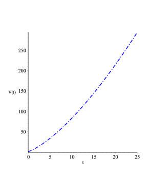
Figure 1: Evolution of the Universe in absence of spinor field (Vacuum solution).

.

As far as spinor field is concerned the Matrix $A$ in (45) in this case becomes trivial and the components of the spinor field can be written as

$$\psi_{i}=\frac{c_{i}}{\sqrt{V}},\quad i=1,\,2,\,3,\,4,$$ (94)

with $c_{i}$’s being the constant of integration obeying

$$c_{1}^{*}c_{1}+c_{2}^{*}c_{2}-c_{3}^{*}c_{3}-c_{4}^{*}c_{4} = 0,$$ (95a)

$$c_{1}^{*}c_{3}+c_{2}^{*}c_{4}-c_{3}^{*}c_{1}-c_{4}^{*}c_{2} = 0.$$ (95b)

The second possibility is to consider (90) with $A^{3}\neq 0$. In this case the nonlinear term as well as the massive term do not vanish. In what follows, we will consider the case for $K=I$, setting

$$F=\sum_{k}\lambda_{k}I^{n_{k}}=\sum_{k}\lambda_{k}S^{2n_{k}}.$$ (96)

As far as other cases are concerned we can revive them setting spinor mass $m_{\rm sp}=0$.

Then inserting (96) into (67) and taking into account that in this case $S=V_{0}/V$ we find

$$\ddot{V}=\Phi_{1}(V),\quad\Phi_{1}=\bar{X}V^{1/3-2/N_{3}}+\frac{3\kappa}{2}\left[m_{\rm sp}\,V_{0}+2\sum_{k}\lambda_{k}(1-n_{k})V_{0}^{2n_{k}}V^{1-2n_{k}}\right],$$ (97)

with the solution in quadrature

$$\frac{dV}{\Phi_{2}}=t+t_{0},\quad\Phi_{2}=\sqrt{\frac{6N_{3}\bar{X}}{4N_{3}-6}V^{(4N_{3}-6)/3N_{3}}+3\kappa\left[m_{\rm sp}\,V_{0}V+\sum_{k}\lambda_{k}V_{0}^{2n_{k}}V^{2(1-n_{k})}\right]+C_{1}},$$ (98)

with $t_{0}$ and $C_{1}$ are being some arbitrary constants.

It can be shown that the metric functions and the components of the spinor field as well as the invariants constructed form them are inverse function of $V$ of some degree, hence at any spacetime point where $V=0$ it is a singularity. So we assume that at the beginning $V$ was small but non-zero. From (97) we see that at initial stage the nonlinear term prevails if $n_{k}=n_{1}$ such that $n_{1}>1/2$ and $n_{1}>1/3+1/N_{3}$, whereas for the nonlinearity to become dominant for large value of $V$ one should have $n_{k}=n_{2}$ such that $n_{2}<1/2$ and $n_{2}<1/3+1/N_{3}$.

In Figs. 2 and 3 we have plotted the evolution of volume scale for positive and negative coupling constants $\lambda_{1}$ and $\lambda_{2}$, respectively. For simplicity we set $m=1$, $X_{0}=1$, $X_{1}=1$, $N_{3}=3$, $m_{\rm sp}=1$, $V_{0}=1$, $\kappa=1$, $C_{1}=10$, $n_{1}=3$, $n_{2}=1/4$ and $N_{3}=3$. In case of positive coupling constants $\lambda_{1}=1$ and $\lambda_{2}=1$ the model describes an expanding Universe, while for negative coupling constants $\lambda_{1}=-0.5$ and $\lambda_{2}=-0.5$ we have a cyclic Universe that expands to some maximum and then contracts to minimum only to expand again. The initial value of volume scale is taken to be $V(0)=0.1$ and $\dot{V}(0)$ is calculated using (98).

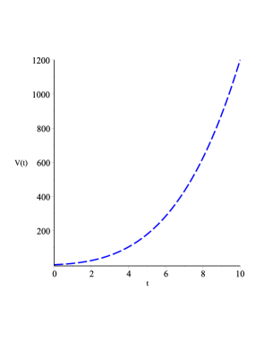
Figure 2: Evolution of the Universe filled with massive spinor field with a positive self-coupling constants $\lambda_{1}=1$ and $\lambda_{2}=1$.

.

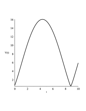
Figure 3: Evolution of the Universe filled with massive spinor field with a negative self-coupling constants $\lambda_{1}=-0.5$ and $\lambda_{2}=-0.5$.

.

Let us also see what happens to deceleration parameter for positive coupling constants. Using the definition

$$q=-\frac{V\ddot{V}}{{\dot{V}}^{2}}=-\frac{V\Phi_{1}}{\Phi_{2}^{2}}$$ (99)

it can be shown that in this case our Universe is expanding with acceleration. Taking into account the discussion about the value of $n_{k}$ we can rewrite

$$q=-\frac{\bar{X}V^{4/3-2/N_{3}}+\frac{3\kappa}{2}\left[m_{\rm sp}\,V_{0}V+2\lambda_{1}(1-n_{1})V_{0}^{2n_{1}}V^{2(1-n_{1})}+2\lambda_{2}(1-n_{2})V_{0}^{2n_{2}}V^{2(1-n_{2})}\right]}{\frac{6N_{3}\bar{X}}{4N_{3}-6}V^{4/3-2/N_{3}}+3\kappa\left[m_{\rm sp}\,V_{0}V+\lambda_{1}V_{0}^{2n_{1}}V^{2(1-n_{1})}+\lambda_{2}V_{0}^{2n_{2}}V^{2(1-n_{2})}\right]+C_{1}}.$$ (100)

As it was mentioned earlier, at large $t$, hence for large $V$ prevails the term with $n_{k}=n_{2}<1/2$. Taking this into account we find

$$\lim_{V\to\infty}q\longrightarrow-(1-n_{2})<0.$$ (101)

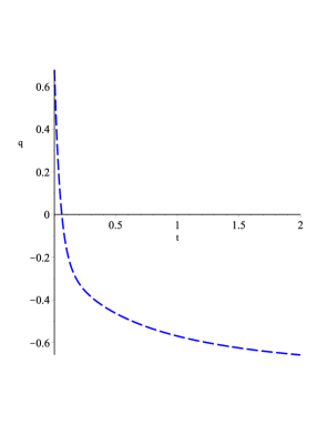
Figure 4: Evolution of the deceleration parameter for the Universe filled with massive spinor field with a positive self-coupling constants $\lambda_{1}=1$ and $\lambda_{2}=1$.

.

In Fig. 4 we have illustrated the evolution of the the deceleration parameter. As we see that the spinor field nonlinearity leads to the late time accelerated expansion of the Universe.

V Conclusion

Within the scope of Bianchi type-$VI_{0}$ spacetime we study the role of spinor field on the evolution of the Universe. In this case we consider the spinor field that depends only on time $t$. Even in this case the spinor field possesses non-zero non-diagonal components of energy-momentum tensor thanks to its specific relation with gravitational field. This fact plays vital role on the evolution of the Universe. Due to the specific behavior of the spinor field we have two different scenarios. In one case the bilinear forms constructed from it becomes trivial, thus giving rise to a massless and linear spinor field Lagrangian. This case is equivalent to the vacuum solution of the Bianchi type-$VI_{0}$ spacetime. The second case allows non-vanishing massive and nonlinear terms and depending on the sign of coupling constants gives rise to expanding mode of expansion or the one that after obtaining some maximum value contracts and ends in big crunch generating spacetime singularity. This result once again shows the sensitivity of spinor field to the gravitational one.

Acknowledgments
This work is supported in part by a joint Romanian-LIT, JINR, Dubna Research Project, theme no. 05-6-1119-2014/2016. I would also like to thank the referee for some valuable suggestions that helped me to improve the MS.

References

- (1) M. Henneaux Phys. Rev. D 21, 857 (1980)
- (2) U. Ochs and M. Sorg Int. J. Theor. Phys. 32, 1531 (1993)
- (3) B. Saha and G.N. Shikin Gen. Relat. Grav. 29, 1099 (1997)
- (4) B. Saha and G.N. Shikin J Math. Phys. 38, 5305 (1997)
- (5) B. Saha Phys. Rev. D 64, 123501 (2001)
- (6) C. Armendriz-Picn and P.B. Greene Gen. Relat. Grav. 35, 1637 (2003)
- (7) B. Saha and T. Boyadjiev Phys. Rev. D 69, 124010 (2004)
- (8) B. Saha Phys. Rev. D 69, 124006 (2004)
- (9) M.O. Ribas, F.P. Devecchi, and G.M. Kremer Phys. Rev. D 72, 123502 (2005)
- (10) B. Saha Phys. Particle. Nuclei. 37. Suppl. 1, S13 (2006)
- (11) B. Saha Phys. Rev. D 74, 124030 (2006)
- (12) B. Saha Grav. Cosmol. 12(2-3)(46-47), 215 (2006)
- (13) B. Saha Romanian Rep. Phys. 59, 649 (2007).
- (14) R.C de Souza and G.M. Kremer Class. Quantum Grav. 25, 225006 (2008)
- (15) N. J. Popławski Phys. Lett. B 690, 73 (2010)
- (16) S. Vignolo, L. Fabbri, and R. Cianci J. Math. Phys. 52 112502 (2011)
- (17) L. Fabbri Phys. Rev. D 85 0475024 (2012)
- (18) N. J. Popławski Phys. Rev. D 85, 107502 (2012)
- (19) N. J. Popławski Gen. Releat. Grav. 44, 1007 (2012)
- (20) L. Fabbri Int. J. Theor. Phys. 52 634 (2013)
- (21) G.M. Kremer and R.C de Souza arXiv:1301.5163v1 [gr-qc]
- (22) B. Saha Int. J. Theor. Phys. 53 1109 (2014)
- (23) B. Saha Astrophys. Space Sci. 357, 28 (2015) DOI 10.1007/s10509-015-2291-x (online first)
- (24) B. Saha and G.N. Shikin Czechoslovak Journal of Physics 54, 597 (2004)
- (25) M. Weaver Classical and Quantum Gravity 17, 421 (2009)
- (26) J. Ibez, R.J. van der Hoogen and A.A. Coley Phys. Rev. D 1995. 51, 928 (1995)
- (27) J. Socorro and E.R. Medina Phys. Rev. D 61, 087702 (2000)
- (28) R. Bali, A. Pradhan and H. Amirhashchi Int. J. Theor. Phys. 47, 2594 (2008)
- (29) J.A. Belinchon Classical and Quantum Gravity 26, 175003 (2009)
- (30) B. Saha Int. J. Theor. Phys. 51, 1812 (2012)
- (31) B. Saha Physics of Particles and Nuclei 45, 349 (2014)
- (32) T.W.B. Kibble J. Math. Phys. 2, 212 (1961)
- (33) K.S. Thorne The Astrophys. J. 148, 51 (1967)
- (34) R. Kantowski and R.K. Sachs J. Math. Phys. 7, 443 (1966)
- (35) J. Kristian and R.K. Sachs Astrophys. J. 143, 379 (1966)
- (36) C. B. Collins, E.N. Glass and D.A. Wilkinson Gen. Rel. Grav. 12, 805 (1980)