Probabilistic representation of a class of non conservative nonlinear Partial Differential Equations

Abstract

We introduce a new class of nonlinear Stochastic Differential Equations in the sense of McKean, related to non conservative nonlinear Partial Differential equations (PDEs). We discuss existence and uniqueness pathwise and in law under various assumptions. We propose an original interacting particle system for which we discuss the propagation of chaos. To this system, we associate a random function which is proved to converge to a solution of a regularized version of PDE.

Key words and phrases: Chaos propagation; Nonlinear Partial Differential Equations; Nonlinear Stochastic Differential Equations; Particle systems; Probabilistic representation of PDEs; McKean.

2010 AMS-classification: 65C05; 65C35; 60H10;60H30; 60J60; 58J35

1 Introduction

Probabilistic representations of nonlinear Partial Differential Equations (PDEs) are interesting in several aspects. From a theoretical point of view, such representations allow for probabilistic tools to study the analytic properties of the equation (existence and/or uniqueness of a solution, regularity,…). They also have their own interest typically when they provide a microscopic interpretation of physical phenomena macroscopically drawn by a nonlinear PDE. Similarly, stochastic control problems are a way of interpreting non-linear PDEs through Hamilton-Jacobi-Bellman equation that have their own theoretical and practical interests (see [16]). Besides, from a numerical point of view, such representations allow for new approximation schemes potentially less sensitive to the dimension of the state space thanks to their probabilistic nature involving Monte Carlo based methods.

The present paper focuses on a specific forward approach relying on nonlinear SDEs in the sense of McKean [22]. The coefficients of that SDE instead of depending only on the position of the solution $Y$, also depend on the law of the process, in a non-anticipating way. One historical contribution on the subject was performed by [31], which concentrated on non-linearities on the drift coefficients.
Let us consider $d,p\in\mathbb{N}^{\star}$. Let $\Phi:[0,T]\times\mathbb{R}^{d}\times\mathbb{R}\rightarrow\mathbb{R}^{d\times p}$, $g:[0,T]\times\mathbb{R}^{d}\times\mathbb{R}\rightarrow\mathbb{R}^{d}$, $\Lambda:[0,T]\times\mathbb{R}^{d}\times\mathbb{R}\rightarrow\mathbb{R}$, be Borel bounded functions and $\zeta_{0}$ be a probability on $\mathbb{R}^{d}$. When it is absolutely continuous we denote by $v_{0}$ its density so that $\zeta_{0}(dx)=v_{0}(x)dx$. We are motivated in non-linear PDEs (in the sense of the distributions) of the form

$$\left\{\begin{array}[]{l}\partial_{t}v=\frac{1}{2}\displaystyle{\sum_{i,j=1}^{d}}\partial_{ij}^{2}\left((\Phi\Phi^{t})_{i,j}(t,x,v)v\right)-div\left(g(t,x,v)v\right)+\Lambda(t,x,v)v\ ,\quad\textrm{for any}\ t\in[0,T]\ ,\\ v(0,dx)=\zeta_{0}(dx),\end{array}\right.$$ (1.1)

where $v:]0,T]\times\mathbb{R}^{d}\rightarrow\mathbb{R}$ is the unknown function and the second equation means that $v(t,x)dx$ converges weakly to $\zeta_{0}(dx)$ when $t\rightarrow 0$. When $\Lambda=0$, PDEs of the type (1.1) are generalizations of the Fokker-Planck equation and they are often denominated in the literature as McKean type equations. Their solutions are probability measures dynamics which often describe the macroscopic distribution law of a microscopic particle which behaves in a diffusive way. For that reason, those time evolution PDEs are conservative in the sense that their solutions $v(t,\cdot)$ verify the property $\int_{\mathbb{R}^{d}}v(t,x)dx$ to be constant in $t$, generally equal to $1$, which is the mass of a probability measure. More precisely, often the solution $v$ of (1.1) is associated with a couple $(Y,v)$, where $Y$ is a stochastic process and $v$ a real valued function defined on $[0,T]\times\mathbb{R}^{d}$ such that

$$\left\{\begin{array}[]{l}Y_{t}=Y_{0}+\int_{0}^{t}\Phi(s,Y_{s},v(s,Y_{s}))dW_{s}+\int_{0}^{t}g(s,Y_{s},v(s,Y_{s}))ds\ ,\quad\textrm{with}\ Y_{0}\sim\zeta_{0}\\ v(t,\cdot)\text{ is the density of the law of }Y_{t}\ ,\end{array}\right.$$ (1.2)

and $(W_{t})_{t\geq 0}$ is a $p$-dimensional Brownian motion on a filtered probability space $(\Omega,\mathcal{F},\mathcal{F}_{t},\mathbb{P})$. A major technical difficulty arising when studying the existence and uniqueness for solutions of (1.2) is due to the point dependence of the SDE coefficients w.r.t. the probability density $v$. In the literature (1.2) was generally faced by analytic methods. A lot of work was performed in the case of smooth Lipschitz coefficients with regular initial condition, see for instance Proposition 1.3. of [20]. The authors also assumed to be in the non-degenerate case, with $\Phi\Phi^{t}$ being an invertible matrix and some parabolicity condition. An interesting earlier work concerns the case $\Phi(t,x,u)=u^{k}\;(k\geq 1),g=0$ see [8]. In dimension $d=1$ with $g=0$ and $\Phi$ being bounded measurable, probabilistic representations of (1.1) via solutions of (1.2) were obtained in [11, 1]. [6] extends partially those results to the multidimensional case. Finally [7] treated the case of fast diffusion. All those techniques were based on the resolution of the corresponding non-linear Fokker-Planck equation, so through an analytic tool.
In the present article, we are however especially interested in (1.1), in the case where $\Lambda$ does not vanish. In that context, the natural generalization of (1.2) is given by

$$\left\{\begin{array}[]{l}Y_{t}=Y_{0}+\int_{0}^{t}\Phi(s,Y_{s},v(s,Y_{s}))dW_{s}+\int_{0}^{t}g(s,Y_{s},v(s,Y_{s}))ds\ ,\quad\textrm{with}\quad Y_{0}\sim\zeta_{0}\ ,\\ v(t,\cdot):=\frac{d\nu_{t}}{dx}\quad\textrm{such that for any bounded continuous test function}\ \varphi\in\mathcal{C}_{b}(\mathbb{R}^{d},\mathbb{R})\\ \nu_{t}(\varphi):=\mathbb{E}\left[\varphi(Y_{t})\,\exp\left\{\int_{0}^{t}\Lambda\big{(}s,Y_{s},v(s,Y_{s})\big{)}ds\right\}\right]\ ,\quad\textrm{for any}\ t\in[0,T]\ .\end{array}\right.$$ (1.3)

The aim of the paper is precisely to extend the McKean probabilistic representation to a large class of nonconservative PDEs. The first step in that direction was done by [2] where the Fokker-Planck equation is a stochastic PDE with multiplicative noise. Even though that equation is pathwise not conservative, the expectation of the mass was constant and equal to $1$. Here again, these developments relied on analytic tools.
To avoid the technical difficulty due to the pointwise dependence of the SDE coefficients w.r.t. the function $v$, this paper focuses on the following regularized version of (1.3):

$$\left\{\begin{array}[]{l}Y_{t}=Y_{0}+\int_{0}^{t}\Phi(s,Y_{s},u(s,Y_{s}))dW_{s}+\int_{0}^{t}g(s,Y_{s},u(s,Y_{s}))ds\ ,\quad\textrm{with}\quad Y_{0}\sim\zeta_{0}\ ,\\ u(t,y):=\mathbb{E}[K(y-Y_{t})\,\exp\left\{\int_{0}^{t}\Lambda\big{(}s,Y_{s},u(s,Y_{s})\big{)}ds\right\}]\ ,\quad\textrm{for any}\ t\in[0,T]\ ,\end{array}\right.$$ (1.4)

where $K:\mathbb{R}^{d}\rightarrow\mathbb{R}$ is a smooth mollifier in $\mathbb{R}^{d}$. When $K=\delta_{0}$ (1.4) reduces, at least formally to (1.3). An easy application of Itô’s formula (see e.g. Proposition 6.7) shows that if there is a solution $(Y,u)$ of (1.4), $u$ is related to the solution (in the distributional sense) of the following partial integro-differential equation (PIDE)

$$\left\{\begin{array}[]{l}\partial_{t}\bar{v}=\frac{1}{2}\displaystyle{\sum_{i,j=1}^{d}}\partial_{ij}^{2}\left((\Phi\Phi^{t})_{i,j}(t,x,K\ast\bar{v})\bar{v}\right)-div\left(g(t,x,K\ast\bar{v})\bar{v}\right)+\Lambda(t,x,K\ast\bar{v})\bar{v}\\ \bar{v}(0,x)=v_{0}\ ,\end{array}\right.$$ (1.5)

by the relation $u=K\ast\bar{v}:=\int_{\mathbb{R}^{d}}K(\cdot-y)\bar{v}(y)dy$. Setting $K^{\varepsilon}(x)=\frac{1}{\varepsilon^{d}}K\left(\frac{\cdot}{\varepsilon}\right)$ the generalized sequence $K^{\varepsilon}$ is weakly convergent to the Dirac measure at zero. Now, consider the couple $(Y^{\varepsilon},u^{\varepsilon})$ solving (1.4) replacing $K$ with $K^{\varepsilon}$. Ideally, $u^{\varepsilon}$ should converge to a solution of the limit partial differential equation (1.1). In the case $\Lambda\equiv 0$, with smooth $\Phi,g$ and initial condition with other technical conditions, that convergence was established in Lemma 2.6 of [20]. In our extended setting, again, no mathematical argument is for the moment available but this limiting behavior is explored empirically by numerical simulations in Section 8. Always in the case $\Lambda=0$ with $g=0$, but with $\Phi$ only measurable, the qualitative behavior of the solution for large time was numerically simulated in [5, 6] respectively for the one-dimensional and multi-dimensional case.

Besides the theoretical aspects related to the well-posedness of (1.1) (and (1.4)), our main motivation is to simulate numerically efficiently their solutions. With this numerical objective, several types of probabilistic representations have been developed in the literature, each one having specific features regarding the implied approximation schemes.
One method which has been largely investigated for approximating solutions of time evolutionary PDEs is the method of forward-backward SDEs. FBSDEs were initially developed in [24], see also [23] for a survey and [25] for a recent monograph on the subject. The idea is to express the PDE solution $v(t,\cdot)$ at time $t$ as the expectation of a functional of the so called forward diffusion process $X$. Numerically, many judicious schemes have been proposed [26, 12, 17]. But they all rely on computing recursively conditional expectation functions which is known to be a difficult task in high dimension. Besides, the FBSDE approach is blind in the sense that the forward process is not ensured to explore the most relevant space regions to approximate efficiently the backward process of interest. On the theoretical side, the FBSDE representation of fully nonlinear PDEs still requires complex developments and is the subject of active research (see for instance [13]).
Branching diffusion processes are another way of providing a probabilistic representation of semi-linear PDEs involving a specific form of non-linearity on the zero order term. We refer to [15] for the case of superprocesses. This type of approach has been recently extended in [18, 19] to a more general class of non-linearities on the zero order term, with the so-called marked branching process. One of the main advantage of this approach compared to BSDEs is that it reduces in a forward algorithm without any regression computation.
One numerical intuition motivating our interest in (possibly non-conservative) PDEs representation of McKean type is the possibility to take advantage of the forward feature of this representation to bypass the dimension problem by localizing the particles precisely in the regions of interest, although this point will not be developed in the present paper. Another benefit of this approach is that it is potentially able to represent fully nonlinear PDEs.

In this paper, for the considered class of nonconservative PDE, besides various theoretical results of existence and uniqueness, we establish the so called propagation of chaos of an associated interacting particle system and we develop a numerical scheme based on it. The convergence of this algorithm is proved by propagation of chaos and through the control of the time discretization error. Finally, some numerical simulations illustrate the practical interest of this new algorithm.

The main contributions of this paper are twofold.

1. We provide a refined analysis of existence and/or uniqueness of a solution to (1.4) under a variety of regularity assumptions on the coefficients $\Phi$, $g$ and $\Lambda$. This analysis faces two main difficulties. In the first equation composing the system (1.4) the coefficients depend on the density $u$, itself depending on $Y$. This is the standard situation already appearing in the context of classical McKean type equations when $u(t,\cdot)$ is characterized by the law of $Y_{t},t\geq 0$. This situation can be recovered formally here when the function $\Lambda\equiv 0$ and the mollifier $K=\delta_{0}$. In the second equation characterizing $u$ in (1.4), for a given process $Y\in\mathcal{C}^{d}:=\mathcal{C}([0,T],\mathbb{R}^{d})$, $u$ also appears on the right-hand-side (r.h.s) via the weighting function $\Lambda$. This additional difficulty is specific to our extended framework since in the standard McKean type equation, $\Lambda\equiv 0$ implies that $u(t,\cdot)$ is explicitely defined by the law density of $Y_{t}$.

   In Section 3, one shows existence and uniqueness of strong solutions of (1.4) when $\Phi,g,\Lambda$ are Lipschitz. This result is stated in Theorem 3.10. The second equation of (1.4) can be rewritten as

   $$u(t,y)=\int_{\mathcal{C}^{d}}K(y-\omega_{t})\exp\left\{\int_{0}^{t}\Lambda\big{(}s,\omega_{s},u(s,\omega_{s})\big{)}ds\right\}dm(\omega)\ ,$$ (1.6)

   where $m=m_{Y}$ is the law of $Y$ on the canonical space $\mathcal{C}^{d}$. In particular, given a law $m$ on $\mathcal{C}^{d}$, using an original fixed point argument on stochastic processes $Z$ of the type $Z_{t}=u(t,X_{t})$ where $X$ is the canonical process, in Lemma 3.2, we first study the existence of $u=u^{m}$ being solution of (1.6). A careful analysis in Lemma 3.4 is carried on the functional $(t,x,m)\mapsto u^{m}(t,x)$: this associates to each Borel probability measure $m$ on ${\cal C}^{d}$, the solution of (3.1), which is the second line of (1.4). In particular that lemma describes carefully the dependence on all variables. Then we consider the first equation of (1.4) using more standard arguments following Sznitman [31]. In Section 4, we show strong existence of (1.4) when $\Phi,g$ are Lipschitz and $\Lambda$ is only continuous, see Theorem 4.2. Indeed, uniqueness, however, does not hold if $\Lambda$ is only continuous, see Example 4.1. In Section 5, Theorem 5.1 states existence in law in all cases when $\Phi,g,\Lambda$ are only continuous.

2. We introduce an interacting particle system associated to (1.4) and prove that the propagation of chaos holds, under the assumptions of Section 3. This is the object of Section 7, see Theorem 7.1 and subsequent remarks. That theorem also states the convergence of the solution $u^{m}$ of (1.6), when $m=S^{N}(\xi)$ is the empirical measure of the particles to $u^{m_{0}}$, where $m_{0}$ is the law of the solution of (1.4), in the $L^{p},p=2,+\infty$ mean error, in term of the number $N$ of particles. We estimate in particular, rates of convergence making use of a refined analysis of the Lipschitz properties of $m\mapsto u^{m}$ w.r.t. various metrics on probability measures. This crucial theorem is an obligatory step in a complete proof of the convergence of the stochastic particle algorithm: it distinguishes clearly the control of the perturbation error induced by the approximation and the control of the propagation of this error through the particle dynamical system. By our techniques, the proof of chaos propagation does not rely on the exchangeability property of the particles. In Section (6) we show that $u:=u^{m_{0}}$ verifies $u:=K\ast\bar{v}$, where $\bar{v}$ solves the PIDE (1.5). In Section 8, we propose an Euler discretization of the particle system dynamics and prove (Proposition 8.1) the convergence of this discrete time approximation to the continuous time interacting particle system by following the same lines of the propagation of chaos analysis, see Theorem 7.1.

The paper is organized as follows. After this introduction, we formulate the basic assumptions valid along the paper. Section 3 is devoted to the existence and uniqueness problem when $\Phi,g,\Lambda$ are Lipschitz. The propagation of chaos is discussed in Section 7. Sections 4 and 5 discuss the case when the coefficients are non-Lipschitz. Section 6 establishes the link between (1.4) and the integro partial-differential equation (1.5). Finally, Section 8 provides numerical simulations illustrating the performances of the interacting particle system in approximating the PDE (1.1), in a specific case where the solution is explicitely known.

2 Notations and assumptions

Let us consider ${\cal C}^{d}:=\mathcal{C}([0,T],\mathbb{R}^{d})$ metrized by the supremum norm $\|\cdot\|_{\infty}$, equipped with its Borel $\sigma-$ field $\mathcal{B}({\cal C}^{d})=\sigma(X_{t},t\geq 0)$ (and $\mathcal{B}_{t}({\cal C}^{d}):=\sigma(X_{u},0\leq u\leq t)$ the canonical filtration) and endowed with the topology of uniform convergence, $X$ the canonical process on ${\cal C}^{d}$ and $\mathcal{P}_{k}({\cal C}^{d})$ the set of Borel probability measures on ${\cal C}^{d}$ admitting a moment of order $k\in\mathbb{N}$. For $k=0$, $\mathcal{P}({\cal C}^{d}):=\mathcal{P}_{0}({\cal C}^{d})$ is naturally the Polish space (with respect to the weak convergence topology) of Borel probability measures on ${\cal C}^{d}$ naturally equipped with its Borel $\sigma$-field $\mathcal{B}({\cal P}({\cal C}^{d}))$. When $d=1$, we often omit it and we simply denote $\mathcal{C}:=\mathcal{C}^{1}$.
We recall that the Wasserstein distance of order $r$ and respectively the modified Wasserstein distance of order $r$ for $r\geq 2$, between $m$ and $m^{\prime}$ in $\mathcal{P}_{r}(\mathcal{C}^{d})$, denoted by $W^{r}_{T}(m,m^{\prime})$ (and resp. $\widetilde{W}^{r}_{T}(m,m^{\prime})$) are such that

$$(W^{r}_{t}(m,m^{\prime}))^{r} := \inf_{\mu\in\Pi(m,m^{\prime})}\left\{\int_{\mathcal{C}^{d}\times\mathcal{C}^{d}}\sup_{0\leq s\leq t}|X_{s}(\omega)-X_{s}(\omega^{\prime})|^{r}d\mu(\omega,\omega^{\prime})\right\},\ t\in[0,T]\ ,$$ (2.1)

$$(\widetilde{W}^{r}_{t}(m,m^{\prime}))^{r} := \inf_{\mu\in\widetilde{\Pi}(m,m^{\prime})}\left\{\int_{\mathcal{C}^{d}\times\mathcal{C}^{d}}\sup_{0\leq s\leq t}|X_{s}(\omega)-X_{s}(\omega^{\prime})|^{r}\wedge 1\;d\mu(\omega,\omega^{\prime})\right\},\ t\in[0,T]\ ,$$ (2.2)

where $\Pi(m,m^{\prime})$ (resp. $\widetilde{\Pi}(m,m^{\prime})$) denotes the set of Borel probability measures in ${\cal P}({\cal C}^{d}\times{\cal C}^{d})$ with fixed marginals $m$ and $m^{\prime}$ belonging to ${\cal P}_{r}({\cal C}^{d})$ (resp. ${\cal P}({\cal C}^{d})$ ). In this paper we will use very frequently the Wasserstein distances of order $2$. For that reason, we will simply denote $W_{t}:=W^{2}_{t}$ (resp. ${\tilde{W}}_{t}:={\tilde{W}}^{2}_{t}$).
Given $N\in\mathbb{N}^{\star}$, $l\in{\cal C}^{d}$, $l^{1},\cdots,l^{N}\in{\cal C}^{d}$, a significant role in this paper will be played by the Borel measures on ${\cal C}^{d}$ given by $\delta_{l}$ and $\displaystyle{\frac{1}{N}\sum_{j=1}^{N}\delta_{l^{j}}}$.

Remark 2.1.

Given $l^{1},\cdots,l^{N},\tilde{l}^{1},\cdots,\tilde{l}^{N}\in{\cal C}^{d}$, by definition of the Wasserstein distance we have, for all $t\in[0,T]$

$$W_{t}\left(\frac{1}{N}\sum_{j=1}^{N}\delta_{l^{j}},\frac{1}{N}\sum_{j=1}^{N}\delta_{\tilde{l}^{j}}\right)\leq\frac{1}{N}\sum_{j=1}^{N}\sup_{0\leq s\leq t}|l^{j}_{s}-\tilde{l}^{j}_{s}|^{2}\ .$$

${\cal C}_{b}({\cal C}^{d})$ will denote the space of bounded, continuous real-valued functions on ${\cal C}^{d}$, for which the supremum norm will also be denoted by $\|\cdot\|_{\infty}$. In the whole paper, $\mathbb{R}^{d}$ will be equipped with the scalar product $\cdot$ and $|x|$ will denote the induced Euclidean norm for $x\in\mathbb{R}^{d}$. $\mathcal{M}_{f}(\mathbb{R}^{d})$ is the space of finite, Borel measures on $\mathbb{R}^{d}$. $\mathcal{S}(\mathbb{R}^{d})$ is the space of Schwartz fast decreasing test functions and $\mathcal{S}^{\prime}(\mathbb{R}^{d})$ is its dual. $\mathcal{C}_{b}(\mathbb{R}^{d})$ is the space of bounded, continuous functions on $\mathbb{R}^{d}$, $\mathcal{C}^{\infty}_{0}(\mathbb{R}^{d})$ is the space of smooth functions with compact support. $\mathcal{C}^{\infty}_{b}(\mathbb{R}^{d})$ is the space of bounded and smooth functions. $\mathcal{C}_{0}(\mathbb{R}^{d})$ will represent the space of continuous functions with compact support in $\mathbb{R}^{d}$. $W^{r,p}(\mathbb{R}^{d})$ is the Sobolev space of order $r\in\mathbb{N}$ in $(L^{p}(\mathbb{R}^{d}),||\cdot||_{p})$, with $1\leq p\leq\infty$. We denote by $(\phi^{d}_{n})_{n\geq 0}$ an usual sequence of mollifiers $\phi^{d}_{n}(x)=\frac{1}{\epsilon_{n}^{d}}\phi^{d}(\frac{x}{\epsilon_{n}})$ where, $\phi^{d}$ is a non-negative function, belonging to the Schwartz space whose integral is $1$ and $(\epsilon_{n})_{n\geq 0}$ a sequence of strictly positive reals verifying $\epsilon_{n}\xrightarrow[\text{$n\longrightarrow\infty$}]{\text{}}0$. When $d=1$, we will simply write $\phi_{n}:=\phi^{1}_{n},\phi:=\phi^{1}.$
$\mathcal{F}(\cdot):f\in\mathcal{S}(\mathbb{R}^{d})\mapsto\mathcal{F}(f)\in\mathcal{S}(\mathbb{R}^{d})$ will denote the Fourier transform on the classical Schwartz space $\mathcal{S}(\mathbb{R}^{d})$ such that for all $\xi\in\mathbb{R}^{d}$,

$$\mathcal{F}(f)(\xi)=\frac{1}{\sqrt{2\pi}}\int_{\mathbb{R}^{d}}f(x)e^{-i\xi\cdot x}dx\ .$$

We will denote in the same manner the corresponing Fourier transform on $\mathcal{S}^{\prime}(\mathbb{R}^{d})$ .
A function $F:[0,T]\times\mathbb{R}^{d}\times\mathbb{R}\rightarrow\mathbb{R}$ will be said continuous with respect to $(y,z)\in\mathbb{R}^{d}\times\mathbb{R}$ (the space variables) uniformly with respect to $t\in[0,T]$ if for every $\varepsilon>0$, there is $\delta>0$, such that $\forall(y,z),(y^{\prime},z^{\prime})\in\mathbb{R}^{d}\times\mathbb{R}$

$$DUnifCont{DUC}|y-y^{\prime}|+|z-z^{\prime}|\leq\delta\Longrightarrow\;\forall t\in[0,T],\;|F(t,y,z)-F(t,y^{\prime},z^{\prime})|\leq\varepsilon.$$ (2.3)

For any Polish space $E$, we will denote by ${\cal B}(E)$ its Borel $\sigma$-field. It is well-known that ${\cal P}(E)$ is also a Polish space with respect to the weak convergence topology, whose Borel $\sigma$-field will be denoted by ${\cal B}({\cal P}(E))$ (see Proposition 7.20 and Proposition 7.23, Section 7.4 Chapter 7 in [9]).
For any fixed measured space $(\Omega,{\cal F})$, a map $\eta:(\Omega,{\cal F})\longrightarrow({\cal P}(E),{\cal B}({\cal P}(E)))$ will be called random measure (or random kernel) if it is measurable. We will denote by ${\cal P}_{2}^{\Omega}(E)$ the space of square integrable random measures, i.e., the space of random measures $\eta$ such that $\mathbb{E}[\eta(E)^{2}]<\infty$.

Remark 2.2.

As highlighted in Remark 3.20 in [14] (see also Proposition 7.25 in [9]), previous definition is equivalent to the two following conditions:

• for each $\bar{\omega}\in\Omega$, $\eta_{\bar{\omega}}\in{\cal P}(E)$,

• for all Borel set $A\in{\cal B}({\cal P}(E))$, $\bar{\omega}\mapsto\eta_{\bar{\omega}}(A)$ is ${\cal F}$-measurable.

Remark 2.3.

Given $\mathbb{R}^{d}$-valued continuous processes $Y^{1},\cdots,Y^{n}$, the application $\displaystyle{\frac{1}{N}\sum_{j=1}^{N}\delta_{Y^{j}}}$ is a random measure on ${\cal P}({\cal C}^{d})$. In fact $\delta_{Y^{j}},1\leq j\leq N$ is a random measure by Remark 2.2.

As mentioned in the introduction $K:\mathbb{R}^{d}\rightarrow\mathbb{R}_{+}$ will be a mollifier such that $\int_{\mathbb{R}^{d}}K(x)dx=1$. Given a finite signed Borel measure $\gamma$ on $\mathbb{R}^{d}$, $K*\gamma$ will denote the convolution function $x\mapsto\gamma(K(x-\cdot))$. In particular if $\gamma$ is absolutely continuous with density ${\dot{\gamma}}$, then $(K*\gamma)(x)=\int_{\mathbb{R}^{d}}K(x-y)\dot{\gamma}(y)dy$. In this article, the following assumptions will be used.

Assumption 1.

1. $\Phi$ and $g$ are Lipschitz functions defined on $[0,T]\times\mathbb{R}^{d}\times\mathbb{R}$ taking values respectively in $\mathbb{R}^{d\times p}$ (space of $d\times p$ matrices) and $\mathbb{R}^{d}$: there exist finite positive reals $L_{\Phi}$ and $L_{g}$ such that for any $(t,y,y^{\prime},z,z^{\prime})\in[0,T]\times\mathbb{R}^{d}\times\mathbb{R}^{d}\times\mathbb{R}\times\mathbb{R}$, we have

   $$|\Phi(t,y^{\prime},z^{\prime})-\Phi(t,y,z)|\leq L_{\Phi}(|z^{\prime}-z|+|y^{\prime}-y|)\quad\textrm{and}\quad|g(t,y^{\prime},z^{\prime})-g(t,y,z)|\leq L_{g}(|z^{\prime}-z|+|y^{\prime}-y|)\ .$$

2. $\Lambda$ is a Borel real valued function defined on $[0,T]\times\mathbb{R}^{d}\times\mathbb{R}$ Lipschitz w.r.t. the space variables: there exists a finite positive real, $L_{\Lambda}$ such that for any $(t,y,y^{\prime},z,z^{\prime})\in[0,T]\times\mathbb{R}^{d}\times\mathbb{R}^{d}\times\mathbb{R}\times\mathbb{R}$, we have

   $$|\Lambda(t,y,z)-\Lambda(t,y^{\prime},z^{\prime})|\leq L_{\Lambda}(|y^{\prime}-y|+|z^{\prime}-z|)\ .$$

3. $\Phi$, $g$ and $\Lambda$ are supposed to be uniformly bounded: there exist finite positive reals $M_{\Phi}$, $M_{g}$ and $M_{\Lambda}$ such that, for any $(t,y,z)\in[0,T]\times\mathbb{R}^{d}\times\mathbb{R}$

   1. $$|\Phi(t,y,z)|\leq M_{\Phi},\quad|g(t,y,z)|\leq M_{g},$$

   2. $$|\Lambda(t,y,z)|\leq M_{\Lambda}\ .$$

4. $K:\mathbb{R}^{d}\rightarrow\mathbb{R}_{+}$ is integrable, Lipschitz, bounded and whose integral is 1: there exist finite positive reals $M_{K}$ and $L_{K}$ such that for any $(y,y^{\prime})\in\mathbb{R}^{d}\times\mathbb{R}^{d}$

   $$|K(y)|\leq M_{K},\quad|K(y^{\prime})-K(y)|\leq L_{K}|y^{\prime}-y|\ \quad\textrm{and}\quad\int_{\mathbb{R}^{d}}K(x)dx=1\ .$$

5. $\zeta_{0}$ is a fixed Borel probability measure on $\mathbb{R}^{d}$ admitting a second order moment.

To simplify we introduce the following notations.

• $V\,:[0,T]\times{\mathcal{C}}^{d}\times\mathcal{C}\rightarrow\mathbb{R}$ defined for any pair of functions $y\in\mathcal{C}^{d}$ and $z\in\mathcal{C}$, by

  $$V_{t}(y,z):=\exp\left(\int_{0}^{t}\Lambda(s,y_{s},z_{s})ds\right)\quad\textrm{for any}\ t\in[0,T]\ .$$ (2.4)

• The real valued process $Z$ such that $Z_{s}=u(s,Y_{s})$, for any $s\in[0,T]$, will often be denoted by $u(Y)$.

With these new notations, the second equation in (1.4) can be rewritten as

$$\nu_{t}(\varphi)=\mathbb{E}[(K\ast\varphi)(Y_{t})V_{t}(Y,u(Y))]\ ,\quad\textrm{for any}\ \varphi\in\mathcal{C}_{b}(\mathbb{R}^{d},\mathbb{R})\ ,\\$$ (2.5)

where $u(t,\cdot)=\frac{d\nu_{t}}{dx}$.

Remark 2.4.

Under Assumption 1. 3.(b), $\Lambda$ is bounded. Consequently

$$0\leq V_{t}(y,z)\leq e^{tM_{\Lambda}}\ ,\quad\textrm{for any}\ (t,y,z)\in[0,T]\times\mathbb{R}^{d}\times\mathbb{R}\ .$$ (2.6)

Under Assumption 1. 2. $\Lambda$ is Lipschitz. Then $V$ inherits in some sense this property. Indeed, observe that for any $(a,b)\in\mathbb{R}^{2}$,

$$e^{b}-e^{a}=(b-a)\int_{0}^{1}e^{\alpha b+(1-\alpha)a}d\alpha\leq e^{\sup(a,b)}|b-a|\ .$$ (2.7)

Then for any continuous functions $y,\,y^{\prime}\in\mathcal{C}^{d}=\mathcal{C}([0,T],\mathbb{R}^{d})$, and $z,\,z^{\prime}\in\mathcal{C}([0,T],\mathbb{R})$, taking $a=\int_{0}^{t}\Lambda(s,y_{s},z_{s})ds$ and $b=\int_{0}^{t}\Lambda(s,y^{\prime}_{s},z^{\prime}_{s})ds$ in the above equality yields

$$|V_{t}(y^{\prime},z^{\prime})-V_{t}(y,z)| \leq e^{tM_{\Lambda}}\int_{0}^{t}\left|\Lambda(s,y^{\prime}_{s},z^{\prime}_{s})-\Lambda(s,y_{s},z_{s})\right|ds$$ (2.8)

$$\leq e^{tM_{\Lambda}}L_{\Lambda}\,\int_{0}^{t}\left(|y^{\prime}_{s}-y_{s}|+|z^{\prime}_{s}-z_{s}|\right)ds\ .$$

In Section 4, Assumption 1. will be replaced by the following.

Assumption 2.

1. All the items of Assumption 1 are in force excepted 2. which is replaced by the following.

2. $\Lambda$ is a real valued function defined on $[0,T]\times\mathbb{R}^{d}\times\mathbb{R}$ continuous w.r.t. the space variables uniformly with respect to the time variable, see e.g. (LABEL:DUC).

Remark 2.5.

The second item in Assumption 2. is fulfilled if the function $\Lambda$ is continuous with respect to $(t,y,z)\in[0,T]\times\mathbb{R}^{d}\times\mathbb{R}$.

In Section 5 we will treat the case when only weak solutions (in law) exist. In this case we will assume the following.

Assumption 3.

All the items of Assumption 1. are in force excepted 5. and the items 1. and 2. which are replaced by the following. $\Phi:[0,T]\times\mathbb{R}^{d}\times\mathbb{R}\longrightarrow\mathbb{R}^{d\times p},\quad g:[0,T]\times\mathbb{R}^{d}\times\mathbb{R}\longrightarrow\mathbb{R}^{d}$ and $\Lambda:[0,T]\times\mathbb{R}^{d}\times\mathbb{R}\rightarrow\mathbb{R}$ are continuous with respect to the space variables uniformly with respect to the time variable.

Definition 2.6.

1. We say that (1.4) admits strong existence if for any filtered probability space $(\Omega,\mathcal{F},\mathcal{F}_{t},\mathbb{P})$ equipped with an $(\mathcal{F}_{t})_{t\geq 0}$-Brownian motion $W$, an ${\cal F}_{0}$-random variable $Y_{0}$ distributed according to $\zeta_{0}$, there is a couple $(Y,u)$ where $Y$ is an $(\mathcal{F}_{t})_{t\geq 0}$-adapted process and $u:[0,T]\times\mathbb{R}^{d}\rightarrow\mathbb{R}$, verifies (1.4).

2. We say that (1.4) admits pathwise uniqueness if for any filtered probability space $(\Omega,\mathcal{F},\mathcal{F}_{t},\mathbb{P})$ equipped with an $(\mathcal{F}_{t})_{t\geq 0}$-Brownian motion $W$, an ${\cal F}_{0}$-random variable $Y_{0}$ distributed according to $\zeta_{0}$, the following holds. Given two pairs $(Y^{1},u^{1})$ and $(Y^{2},u^{2})$ as in item 1., verifying (1.4) such that $Y^{1}_{0}=Y^{2}_{0}$ $\mathbb{P}$-a.s. then $u^{1}=u^{2}$ and $Y^{1}$ and $Y^{2}$ are indistinguishable.

Definition 2.7.

1. We say that (1.4) admits existence in law (or weak existence) if there is a filtered probability space $(\Omega,\mathcal{F},\mathcal{F}_{t},\mathbb{P})$ equipped with an $(\mathcal{F}_{t})_{t\geq 0}$-Brownian motion $W$, a pair $(Y,u)$, verifying (1.4), where $Y$ is an $(\mathcal{F}_{t})_{t\geq 0}$-adapted process and $u$ is a real valued function defined on $[0,T]\times\mathbb{R}^{d}$.

2. We say that (1.4) admits uniqueness in law (or weak uniqueness), if the following holds. Let $(\Omega,\mathcal{F},\mathcal{F}_{t},\mathbb{P})$ (resp. $(\tilde{\Omega},\tilde{\mathcal{F}},\tilde{\mathcal{F}}_{t},\tilde{\mathbb{P}})$) be a filtered probability space. Let $(Y^{1},u^{1})$ (resp. $(\tilde{Y}^{2},\tilde{u}^{2})$) be a solution of (1.4). Then $u^{1}=\tilde{u}^{2}$ and $Y^{1}$ and $\tilde{Y}^{2}$ have the same law.

3 Existence and uniqueness of the problem in the Lipschitz case

In this section we will fix a probability space $(\Omega,{\mathcal{F}},{\mathcal{F}}_{t},\mathbb{P})$ equipped with an $({\mathcal{F}}_{t})$-Brownian motion $(W_{t})$. We will proceed in two steps. We study first in the next section the second equation of (1.4) defining $u$. Then we will address the main equation defining the process $Y$.

Later in this section, Assumption 1 will be in force, in particular $\zeta_{0}$ will be supposed to have a second order moment.

3.1 Existence and uniqueness of a solution to the linking equation

This subsection relies only on items $2.$, $3.(b)$ and $4.$ of Assumption 1.
We remind that $X$ will denote the canonical process $X:{\mathcal{C}}^{d}\rightarrow{\mathcal{C}^{d}}$ defined by $X_{t}(\omega)=\omega(t),\ t\geq 0,\omega\in{\mathcal{C}^{d}}$.

For a given probability measure $m\in\mathcal{P}(\mathcal{C}^{d})$, let us consider the equation

$$\left\{\begin{array}[]{l}u(t,y)=\int_{\mathcal{C}^{d}}K(y-X_{t}(\omega))V_{t}(X(\omega),u(X(\omega)))dm(\omega)\ ,\quad\textrm{for all}\quad t\in[0,T],y\in\mathbb{R}^{d}\ ,\quad\textrm{with}\\ \\ V_{t}(X(\omega),u(X(\omega)))=\exp\left(\int_{0}^{t}\Lambda\big{(}s,X_{s}(\omega),u(s,X_{s}(\omega))\big{)}ds\right)\ .\end{array}\right.$$ (3.1)

This equation will be called linking equation: it constitutes the second line of equation (1.4). When $\Lambda=0$, i.e. in the conservative case, $u(t,\cdot)=K*m_{t}$, where $m_{t}$ is the marginal law of $X_{t}$ under $m$. Informally speaking, when $K$ is the Delta Dirac measure, then $u(t,\cdot)=m_{t}$.

Remark 3.1.

Since $\Lambda$ is bounded, and $K$ Lipschitz, it is clear that if $u:=u^{m}$ is a solution of (3.1) then $u$ is necessarily bounded by a constant, only depending on $M_{\Lambda},M_{K},T$ and it is Lipschitz with respect to the second argument with Lipschitz constant only depending on $L_{K},M_{\Lambda},T$.

We aim at proving by a fixed point argument the following result.

Lemma 3.2.

We assume the validity of items $2.$, $3.(b)$ and $4.$ of Assumption 1.
For a given probability measure $m\in\mathcal{P}(\mathcal{C}^{d})$, equation (3.1) admits a unique solution, $u^{m}$.

Proof.

Let us introduce the linear space $\mathcal{C}_{1}$ of real valued continuous processes $Z$ on $[0,T]$ (defined on the canonical space $\mathcal{C}^{d}$) such that

$$\|Z\|_{\infty,1}:=\mathbb{E}^{m}\,\left[\,\sup_{t\leq T}|Z_{t}|\,\right]:=\int_{\mathcal{C}^{d}}\;\sup_{0\leq t\leq T}|Z_{t}(\omega)|dm(\omega)<\infty\ .$$

$(\mathcal{C}_{1},\|\cdot\|_{\infty,1})$ is a Banach space. For any $M\geq 0$, a well-known equivalent norm to $\|\cdot\|_{\infty,1}$ is given by $\|\cdot\|^{M}_{\infty,1}$, where $\|Z\|^{M}_{\infty,1}=\mathbb{E}^{m}\,[\,\sup_{t\leq T}\,e^{-Mt}|Z_{t}|\,].$ Let us define the operator $T^{m}:\mathcal{C}_{1}\rightarrow\mathcal{C}([0,T]\times\mathbb{R}^{d},\mathbb{R})$ such that for any $Z\in\mathcal{C}_{1}$,

$$T^{m}(Z)(t,y):=\int_{\mathcal{C}^{d}}K\big{(}y-X_{t}(\omega)\big{)}V_{t}\big{(}X(\omega),Z(\omega)\big{)}dm(\omega)\ .$$ (3.2)

Then we introduce the operator $\tau:f\in\mathcal{C}([0,T]\times\mathbb{R}^{d},\mathbb{R})\mapsto\tau(f)\in\mathcal{C}_{1}$, where $\tau(f)_{t}(\omega)=f(t,\omega_{t})$. We observe that $\tau\circ T^{m}$ is a map $\mathcal{C}_{1}\rightarrow\mathcal{C}_{1}$.

Notice that equation (3.1) is equivalent to

$$u=(T^{m}\circ\tau)(u).$$ (3.3)

We first admit the existence and uniqueness of a fixed point $Z\in{\mathcal{C}}_{1}$ for the map $\tau\circ T^{m}$. In particular we have $Z=(\tau\circ T^{m})(Z)$. We can now deduce the existence/uniqueness for the function $u$ for problem (3.3).
Concerning existence, we choose $v^{m}:=T^{m}(Z)$. Since $Z$ is a fixed-point of the map $\tau\circ T^{m}$, by the definition of $v^{m}$ we have

$$Z=\tau(T^{m}(Z)),$$ (3.4)

so that $v^{m}$ is a solution of (3.3).
Concerning uniqueness of (3.3), we consider two solutions of (3.1) $\bar{v},\tilde{v}$, i.e. such that $\bar{v}=(T^{m}\circ\tau)(\bar{v}),\tilde{v}=(T^{m}\circ\tau)(\tilde{v})$. We set $\bar{Z}:=\tau(\bar{v}),\tilde{Z}:=\tau(\tilde{v})$. Since $\bar{v}=T^{m}(\bar{Z})$ we have $\bar{Z}=\tau(\bar{v})=\tau(T^{m}(\bar{Z}))$. Similarly $\tilde{Z}=\tau(\tilde{v})=\tau(T^{m}(\tilde{Z}))$. Since $\bar{Z}$ and $\tilde{Z}$ are fixed points of $\tau\circ T$, it follows that $\bar{Z}=\tilde{Z}\ dm$ a.e. Finally $\bar{v}=T^{m}(\bar{Z})=T^{m}(\tilde{Z})=\tilde{v}$.

It remains finally to prove that $\tau\circ T^{m}$ admits a unique fixed point, $Z$.
The upper bound (2.8) implies that for any pair $(Z,Z^{\prime})\in\mathcal{C}_{1}\times\mathcal{C}_{1}$, for any $(t,y)\in[0,T]\times\mathbb{R}^{d}$,

$$|T^{m}(Z^{\prime})-T^{m}(Z)|(t,y) = \left|\int_{\mathcal{C}^{d}}K(y-X_{t}(\omega))\left[V_{t}(X(\omega),Z^{\prime}(\omega))-V_{t}(X(\omega),Z(\omega))\right]dm(\omega)\right|\$$

$$\leq M_{K}e^{tM_{\Lambda}}L_{\Lambda}\int_{\mathcal{C}^{d}}\int_{0}^{t}|Z^{\prime}_{s}(\omega)-Z_{s}(\omega)|ds\,dm(\omega)$$

$$\leq M_{K}e^{TM_{\Lambda}}L_{\Lambda}\mathbb{E}\left[\int_{0}^{t}e^{Ms}e^{-Ms}|Z^{\prime}_{s}-Z_{s}|ds\right]$$

$$\leq M_{K}e^{TM_{\Lambda}}L_{\Lambda}\mathbb{E}\left[\int_{0}^{t}e^{Ms}\sup_{r\leq t}e^{-Mr}|Z^{\prime}_{r}-Z_{r}|ds\right]$$

$$\leq M_{K}e^{TM_{\Lambda}}L_{\Lambda}\frac{e^{Mt}-1}{M}\mathbb{E}\left[\sup_{r\leq t}e^{-Mr}|Z^{\prime}_{r}-Z_{r}|\right]$$

$$\leq M_{K}e^{TM_{\Lambda}}L_{\Lambda}\frac{e^{Mt}-1}{M}\|Z^{\prime}-Z\|_{\infty,1}^{M}\ .$$

Then considering $(\tau\circ T^{m})(Z^{\prime})_{t}=T^{m}((Z^{\prime})(t,X_{t})$ and $(\tau\circ T^{m})(Z)_{t}=T(Z)(t,X_{t})$, we obtain

$$\sup_{t\leq T}e^{-Mt}\left|(\tau\circ T^{m})(Z^{\prime})_{t}-(\tau\circ T^{m})(Z)_{t}\right| = \sup_{t\leq T}e^{-Mt}\left|T^{m}(Z^{\prime})(t,X_{t})-T^{m}(Z)(t,X_{t})\right|$$

$$\leq M_{K}e^{TM_{\Lambda}}L_{\Lambda}\frac{1}{M}\|Z^{\prime}-Z\|^{M}_{\infty,1}\ .$$

Taking the expectation yields $|(\tau\circ T^{m})(Z^{\prime})_{t}-(\tau\circ T^{m})(Z)_{t}\|^{M}_{\infty,1}\leq M_{K}e^{TM_{\Lambda}}L_{\Lambda}\frac{1}{M}\|Z^{\prime}-Z\|^{M}_{\infty,1}$. Hence, as soon as $M$ is sufficiently large, $M>M_{K}e^{TM_{\Lambda}}L_{\Lambda}$, $(\tau\circ T^{m})$ is a contraction on $(\mathcal{C}_{1},\|\cdot\|^{M}_{\infty,1})$ and the proof ends by a simple application of the Banach fixed point theorem. ∎

Remark 3.3.

For $(y,m)\in\mathbb{R}^{d}\times\mathcal{P}(\mathcal{C}^{d})$, $t\mapsto u^{m}(t,y)$ is continuous. This follows by an application of Lebesgue dominated convergence theorem in (3.1).

In the sequel, we will need a stability result on $u^{m}$ solution of (3.1), w.r.t. the probability measure $m$.

The fundamental lemma treats this issue, again only supposing the validity of items $2.$, $3.(b)$ and $4.$ of Assumption 1.

Lemma 3.4.

We assume the validity of items $2.$, $3.(b)$ and $4.$ of Assumption 1.
Let $u$ be a solution of (3.1). The following assertions hold.

1. For any measures $(m,m^{\prime})\in\mathcal{P}_{2}(\mathcal{C}^{d})\times\mathcal{P}_{2}(\mathcal{C}^{d})$, for all $(t,y,y^{\prime})\in[0,T]\times{\cal C}^{d}\times{\cal C}^{d}$, we have

   $$|u^{m}\big{(}t,y\big{)}-u^{m^{\prime}}\big{(}t,y^{\prime}\big{)}|^{2}\leq C_{K,\Lambda}(t)\left[|y-y^{\prime}|^{2}+|W_{t}(m,m^{\prime})|^{2}\right]\ ,$$ (3.5)

   where $C_{K,\Lambda}(t):=2C^{\prime}_{K,\Lambda}(t)(t+2)(1+e^{2tC^{\prime}_{K,\Lambda}(t)})$ with $C^{\prime}_{K,\Lambda}(t)=2e^{2tM_{\Lambda}}(L^{2}_{K}+2M^{2}_{K}L^{2}_{\Lambda}t)$. In particular the functions $C_{K,\Lambda}$ only depend on $M_{K},L_{K},M_{\Lambda},L_{\Lambda}$ and $t$ and is increasing with $t$.

2. For any measures $(m,m^{\prime})\in{\cal P}(C^{d})\times{\cal P}(C^{d})$, for all $(t,y,y^{\prime})\in[0,T]\times{\cal C}^{d}\times{\cal C}^{d}$, we have

   $$|u^{m}\big{(}t,y\big{)}-u^{m^{\prime}}\big{(}t,y^{\prime}\big{)}|^{2}\leq\mathfrak{C}_{K,\Lambda}(t)\left[|y-y^{\prime}|^{2}+|\widetilde{W}_{t}(m,m^{\prime})|^{2}\right]\ ,$$ (3.6)

   where $\mathfrak{C}_{K,\Lambda}(t):=2e^{2tM_{\Lambda}}(\max(L_{K},2M_{K})^{2}+2M_{K}^{2}\max(L_{\Lambda},2M_{\Lambda})^{2}t)$.

3. The function $(m,t,x)\mapsto u^{m}(t,y)$ is continuous on ${\cal P}({\cal C}^{d})\times[0,T]\times\mathbb{R}^{d}$ where ${\cal P}({\cal C}^{d})$ is endowed with the topology of weak convergence.

4. Suppose that $K\in W^{1,2}(\mathbb{R}^{d})$. Then for any $(m,m^{\prime})\in\mathcal{P}_{2}(\mathcal{C}^{d})\times\mathcal{P}_{2}(\mathcal{C}^{d})$, $t\in[0,T]$

   $$\|u^{m}(t,\cdot)-u^{m^{\prime}}(t,\cdot)\|_{2}^{2}\leq\tilde{C}_{K,\Lambda}(t)(1+2tC_{K,\Lambda}(t))|W_{t}(m,m^{\prime})|^{2}\ ,$$ (3.7)

   where $C_{K,\Lambda}(t):=2C^{\prime}_{K,\Lambda}(t)(t+2)(1+e^{2tC^{\prime}_{K,\Lambda}(t)})$ with $C^{\prime}_{K,\Lambda}(t)=2e^{2tM_{\Lambda}}(L^{2}_{K}+2M^{2}_{K}L^{2}_{\Lambda}t)$ and $\tilde{C}_{K,\Lambda}(t):=2e^{2tM_{\Lambda}}(2M_{K}L_{\Lambda}^{2}t(t+1)+\|\nabla K\|_{2}^{2})$, $\|\cdot\|_{2}$ being the standard $L^{2}(\mathbb{R}^{d})$ or $L^{2}(\mathbb{R}^{d},\mathbb{R}^{d})$-norms.
   In particular the functions $\tilde{C}_{K,\Lambda}$ only depend on $M_{K},L_{K},M_{\Lambda},L_{\Lambda}$ and $t$ and is increasing with $t$.

5. Suppose that ${\cal F}(K)\in L^{1}(\mathbb{R}^{d})$. Then there exists a constant $\bar{C}_{K,\Lambda}(t)>0$ (depending only on $t,M_{\Lambda},L_{\Lambda},\|{\cal F}(K)\|_{1}$) such that for any random measure $\eta:(\Omega,{\cal F})\longrightarrow({\cal P}_{2}({\cal C}^{d}),{\cal B}({\cal P}({\cal C}^{d})))$, for all $(t,m)\in[0,T]\times{\cal P}_{2}({\cal C}^{d})$

   $$\mathbb{E}{[\|u^{\eta}(t,\cdot)-u^{m}(t,\cdot)\|_{\infty}^{2}]} \leq \bar{C}_{K,\Lambda}(t)\sup_{\underset{\|\varphi\|_{\infty}\leq 1}{\varphi\in{\cal C}_{b}({\cal C}^{d})}}\mathbb{E}{[|\langle\eta-m,\varphi\rangle|^{2}]}\ ,$$ (3.8)

   where we recall that ${\cal P}({\cal C}^{d})$ is endowed with the topology of weak convergence. We remark that the expectation in both sides of (3.8) is taken w.r.t. the randomness of the random measure $\eta$.

Remark 3.5.

1. By Corollary 6.13, Chapter 6 in [32], $\widetilde{W}_{T}$ is a metric compatible with the weak convergence on ${\cal P}({\cal C}^{d})$.

2. The map $\displaystyle{d_{2}^{\Omega}:(\nu,\mu)\mapsto\sqrt{\sup_{\underset{\|\varphi\|_{\infty}\leq 1}{\varphi\in{\cal C}_{b}({\cal C}^{d})}}\mathbb{E}[|\langle\nu-\mu,\varphi\rangle|^{2}]}}$ defines a (homogeneous) distance on ${\cal P}_{2}^{\Omega}({\cal C}^{d})$.

3. Previous distance satisfies

   $$d_{2}^{\Omega}(\nu,\mu)\leq\sqrt{\mathbb{E}[|W_{T}^{1}(\nu,\mu)|^{2}]}\ ,$$ (3.9)

   where $W^{1}_{T}$ is the $1$-Wasserstein distance.
   Indeed, for fixed $\bar{\omega}\in\Omega$, taking into account that $({\cal C}^{d},\nu_{\bar{\omega}})$ and $({\cal C}^{d},\mu_{\bar{\omega}})$ are Polish probability spaces, the first equality of (i) in the Kantorovitch duality theorem, see Theorem 5.10 p.70 in [32], which in particular implies the following. For any $\varphi\in{\cal C}_{b}({\cal C}^{d})$ we have

   $$|\langle\nu-\mu,\varphi\rangle|\leq W_{T}^{1}(\nu,\mu),$$

   which implies (3.9).

4. The map $(\nu,\mu)\mapsto\sqrt{\mathbb{E}[|W_{T}^{1}(\nu,\mu)|^{2}]}$ defines a distance on ${\cal P}_{2}^{\Omega}({\cal C}^{d})$.

5. Item 1. of Lemma 3.4 is a consequence of item 2. For expository reasons, we have decided to start with the less general case.

Proof of Lemma 3.4.

We will prove successively the inequalities (3.5), (3.6), (3.7) and (3.8).
Let us consider $(t,y,y^{\prime})\in[0,T]\times\mathbb{R}^{d}\times\mathbb{R}^{d}$.

• Proof of (3.5) . Let $(m,m^{\prime})\in\mathcal{P}_{2}(\mathcal{C}^{d})\times\mathcal{P}_{2}(\mathcal{C}^{d})$.
  We have

  $$|u^{m}(t,y)-u^{m^{\prime}}(t,y^{\prime})|^{2}\leq 2|u^{m}(t,y)-u^{m}(t,y^{\prime})|^{2}+2|u^{m}(t,y^{\prime})-u^{m^{\prime}}(t,y^{\prime})|^{2}\ .$$ (3.10)

  The first term on the r.h.s. of the above equality is bounded using the Lipschitz property of $u^{m}$ that derives straightforwardly from the Lipschitz property of the mollifier $K$ and the boundedness property of $V_{t}$ (2.6):

  $$|u^{m}(t,y^{\prime})-u^{m}(t,y)| = \left|\int_{\mathcal{C}^{d}}\left[K(y-X_{t}(\omega))-K(y^{\prime}-X_{t}(\omega))\right]V_{t}(X(\omega),u^{m}(X(\omega)))dm(\omega)\right|$$ (3.11)

  $$\leq L_{K}e^{tM_{\Lambda}}|y-y^{\prime}|\ .$$

  Now let us consider the second term on the r.h.s of (3.10). By Jensen’s inequality we get

  $$|u^{m}(t,y^{\prime})-u^{m^{\prime}}(t,y^{\prime})|^{2} = \left|\int_{\mathcal{C}^{d}}K(y^{\prime}-X_{t}(\omega))V_{t}\big{(}X(\omega),u^{m}(X(\omega))\big{)}dm(\omega)\right.$$ (3.12)

  $$\left.-\int_{\mathcal{C}^{d}}K(y^{\prime}-X_{t}(\omega^{\prime}))V_{t}\big{(}X(\omega^{\prime}),u^{m^{\prime}}(X(\omega^{\prime}))\big{)}dm^{\prime}(\omega^{\prime})\right|^{2}$$

  $$\leq \int_{\mathcal{C}^{d}\times\mathcal{C}^{d}}\Big{|}K(y^{\prime}-X_{t}(\omega))V_{t}\big{(}X(\omega),u^{m}(X(\omega))\big{)}$$

  $$-\;K(y^{\prime}-X_{t}(\omega^{\prime}))V_{t}\big{(}X(\omega^{\prime}),u^{m^{\prime}}(X(\omega^{\prime}))\big{)}\Big{|}^{2}d\mu(\omega,\omega^{\prime})\ ,$$

  for any $\mu\in\Pi(m,m^{\prime})$. Let us consider four continuous functions $x,\,x^{\prime}\in\mathcal{C}([0,T],\mathbb{R}^{d})$ and $z,z^{\prime}\in\mathcal{C}([0,T],\mathbb{R})$. We have

  $$\left|K(y^{\prime}-x_{t})V_{t}(x,z)-K(y^{\prime}-x^{\prime}_{t})V_{t}(x^{\prime},z^{\prime})\right|^{2} \leq 2\left|K(y^{\prime}-x_{t})-K(y^{\prime}-x^{\prime}_{t})\right|^{2}|V_{t}(x,z)|^{2}$$ (3.13)

  $$+2\left|V_{t}(x,z)-V_{t}(x^{\prime},z^{\prime})\right|^{2}|K(y^{\prime}-x^{\prime}_{t})|^{2}\ .$$

  Then, using the Lipschitz property of $K$ and the upper bound (2.8) gives

  $$\left|K(y^{\prime}-x_{t})V_{t}(x,z)-K(y^{\prime}-x^{\prime}_{t})V_{t}(x^{\prime},z^{\prime})\right|^{2} \leq 2L^{2}_{K}e^{2tM_{\Lambda}}|x_{t}-x^{\prime}_{t}|^{2}$$

  $$+ 4M^{2}_{K}L^{2}_{\Lambda}e^{2tM_{\Lambda}}t\int_{0}^{t}\left[|x_{s}-x^{\prime}_{s}|^{2}+|z_{s}-z^{\prime}_{s}|^{2}\right]\,ds$$

  $$\leq C^{\prime}_{K,\Lambda}(t)\left[(1+t)\sup_{s\leq t}|x_{s}-x^{\prime}_{s}|^{2}+\int_{0}^{t}|z_{s}-z^{\prime}_{s}|^{2}\,ds\right]\ ,$$

  where $C^{\prime}_{K,\Lambda}(t)=2e^{2tM_{\Lambda}}(L^{2}_{K}+2M^{2}_{K}L^{2}_{\Lambda}t)$. Injecting the latter inequality in (3.12) yields

  $$|u^{m}(t,y^{\prime})-u^{m^{\prime}}(t,y^{\prime})|^{2} \leq C^{\prime}_{K,\Lambda}(t)\int_{\mathcal{C}^{d}\times\mathcal{C}^{d}}\left[(1+t)\sup_{s\leq t}|X_{s}(\omega)-X_{s}(\omega^{\prime})|^{2}\right.$$

  $$\left.+\int_{0}^{t}|u^{m}(s,X_{s}(\omega))-u^{m^{\prime}}(s,X_{s}(\omega^{\prime}))|^{2}\,ds\right]d\mu(\omega,\omega^{\prime})\ ,$$

  Injecting the above inequality in (3.10) and using (3.11) yields

  $$|u^{m}(t,y)-u^{m^{\prime}}(t,y^{\prime})|^{2} \leq 2C^{\prime}_{K,\Lambda}(t)\left[|y-y^{\prime}|^{2}+(1+t)\int_{\mathcal{C}^{d}\times\mathcal{C}^{d}}\sup_{s\leq t}|X_{s}(\omega)-X_{s}(\omega^{\prime})|^{2}d\mu(\omega,\omega^{\prime})\right.$$ (3.15)

  $$\left.+\int_{\mathcal{C}^{d}\times\mathcal{C}^{d}}\int_{0}^{t}|u^{m}(s,X_{s}(\omega))-u^{m^{\prime}}(s,X_{s}(\omega^{\prime}))|^{2}\,ds\,d\mu(\omega,\omega^{\prime})\right]\ ,$$

  Replacing $y$ (resp. $y^{\prime}$) with $X_{t}(\omega)$ (resp. $X_{t}(\omega^{\prime})$) in (3.15), we get for all $\omega\in\mathcal{C}^{d}$ (resp. $\omega^{\prime}\in\mathcal{C}^{d}$),

  $$|u^{m}(t,X_{t}(\omega))-u^{m^{\prime}}(t,X_{t}(\omega^{\prime}))|^{2} \leq 2C^{\prime}_{K,\Lambda}(t)\Big{[}|X_{t}(\omega)-X_{t}(\omega^{\prime})|^{2}$$

  $$+(1+t)\int_{\mathcal{C}^{d}\times\mathcal{C}^{d}}\displaystyle{\sup_{s\leq t}}|X_{s}(\omega)-X_{s}(\omega^{\prime})|^{2}d\mu(\omega,\omega^{\prime})$$

  $$+\int_{\mathcal{C}^{d}\times\mathcal{C}^{d}}\int_{0}^{t}|u^{m}(s,X_{s}(\omega))-u^{m^{\prime}}(s,X_{s}(\omega^{\prime}))|^{2}\,ds\,d\mu(\omega,\omega^{\prime})\Big{]}.$$

  Let us introduce the following notation

  $$\gamma(s):=\int_{\mathcal{C}^{d}\times\mathcal{C}^{d}}|u^{m}(s,X_{s}(\omega))-u^{m^{\prime}}(s,X_{s}(\omega^{\prime}))|^{2}\,d\mu(\omega,\omega^{\prime})\ ,\quad\textrm{for any}\ s\in[0,T].\$$

  Integrating each side of inequality (• ‣ 3.1) w.r.t. the variables $(\omega,\omega^{\prime})$ according to $\mu$, implies

  $$\gamma(t)\leq 2C^{\prime}_{K,\Lambda}(t)\int_{0}^{t}\gamma(s)ds+2(t+2)C^{\prime}_{K,\Lambda}(t)\int_{\mathcal{C}^{d}\times\mathcal{C}^{d}}\sup_{s\leq t}|X_{s}(\omega)-X_{s}(\omega^{\prime})|^{2}d\mu(\omega,\omega^{\prime})\ ,$$

  for all $t\in[0,T]$. In particular, observing that $C^{\prime}_{K,\Lambda}(a)$ is increasing in $a$, we have for fixed $t\in]0,T]$ and all $a\in[0,t]$

  $$\gamma(a)\leq 2C^{\prime}_{K,\Lambda}(t)\int_{0}^{a}\gamma(s)ds+2(t+2)C^{\prime}_{K,\Lambda}(t)\int_{\mathcal{C}^{d}\times\mathcal{C}^{d}}\sup_{s\leq t}|X_{s}(\omega)-X_{s}(\omega^{\prime})|^{2}d\mu(\omega,\omega^{\prime})\ .$$

  Using Gronwall’s lemma yields

  $$\gamma(t) := \int_{\mathcal{C}^{d}\times\mathcal{C}^{d}}|u^{m}(t,X_{t}(\omega))-u^{m^{\prime}}(t,X_{t}(\omega^{\prime}))|^{2}\,d\mu(\omega,\omega^{\prime})$$

  $$\leq 2(t+2)C^{\prime}_{K,\Lambda}(t)e^{2tC^{\prime}_{K,\Lambda}(t)}\int_{\mathcal{C}^{d}\times\mathcal{C}^{d}}\sup_{s\leq t}|X_{s}(\omega)-X_{s}(\omega^{\prime})|^{2}d\mu(\omega,\omega^{\prime})\ .$$

  Injecting the above inequality in (3.15) implies

  $$|u^{m}(t,y)-u^{m^{\prime}}(t,y^{\prime})|^{2}\leq 2C^{\prime}_{K,\Lambda}(t)(t+2)(1+e^{2tC^{\prime}_{K,\Lambda}(t)})\left[|y-y^{\prime}|^{2}+\int_{\mathcal{C}^{d}\times\mathcal{C}^{d}}\sup_{s\leq t}|X_{s}(\omega)-X_{s}(\omega^{\prime})|^{2}d\mu(\omega,\omega^{\prime})\right]\ .$$

  The above inequality holds for any $\mu\in\Pi(m,m^{\prime})$, hence taking the infimum over $\mu\in\Pi(m,m^{\prime})$ concludes the proof of (3.5).
  

• Proof of (3.6). Let $(m,m^{\prime})\in\mathcal{P}(\mathcal{C}^{d})\times\mathcal{P}(\mathcal{C}^{d})$. The proof of (3.6) follows at the beginning the same lines as the one of (3.5), but the inequality (• ‣ 3.1) is replaced by

  $$\left|K(y^{\prime}-x_{t})V_{t}(x,z)-K(y^{\prime}-x^{\prime}_{t})V_{t}(x^{\prime},z^{\prime})\right|^{2} \leq 2\left|K(y^{\prime}-x_{t})-K(y^{\prime}-x^{\prime}_{t})\right|^{2}|V_{t}(x,z)|^{2}$$

  $$+2\left|V_{t}(x,z)-V_{t}(x^{\prime},z^{\prime})\right|^{2}|K(y^{\prime}-x^{\prime}_{t})|^{2}$$

  $$\leq 2e^{2tM_{\Lambda}}\max(L_{K},2M_{K})^{2}(\left|x_{t}-x^{\prime}_{t}\right|^{2}\wedge 1)$$

  $$+4M_{K}^{2}e^{2tM_{\Lambda}}\max(L_{\Lambda},2M_{\Lambda})^{2}t\int_{0}^{t}\Big{(}|x_{s}^{\prime}-x_{s}|^{2}\wedge 1$$

  $$+\;|z_{s}-z^{\prime}_{s}|^{2}\Big{)}ds$$

  $$\leq \mathfrak{C}_{K,\Lambda}(t)\left[(1+t)(\sup_{s\leq t}|x_{s}-x^{\prime}_{s}|^{2}\wedge 1)+\int_{0}^{t}|z_{s}-z^{\prime}_{s}|^{2}\,ds\right],$$

  which implies

  $$|u^{m}(t,y)-u^{m^{\prime}}(t,y^{\prime})|^{2} \leq 2\mathfrak{C}_{K,\Lambda}(t)(t+2)(1+e^{2t\mathfrak{C}_{K,\Lambda}(t)})\Big{[}\;|y-y^{\prime}|^{2}$$ (3.18)

  $$+\int_{\mathcal{C}^{d}\times\mathcal{C}^{d}}\sup_{s\leq t}|X_{s}(\omega)-X_{s}(\omega^{\prime})|^{2}\wedge 1\;d\mu(\omega,\omega^{\prime})\Big{]}\ ,$$

  where $\mathfrak{C}_{K,\Lambda}(t):=2e^{2tM_{\Lambda}}(\max(L_{K},2M_{K})^{2}+2M_{K}^{2}\max(L_{\Lambda},2M_{\Lambda})^{2}t)$. This gives the analogue of (3.15) and we conclude in the same way as for the previous item.

• Proof of the continuity of $(m,t,x)\mapsto u^{m}(t,x)$.
  ${\cal P}({\cal C}^{d})\times[0,T]\times\mathbb{R}^{d}$ being a separable metric space, we characterize the continuity through converging sequences. We also recall that $\widetilde{W}_{T}$ is a metric compatible with the weak convergence on ${\cal P}({\cal C}^{d})$, see Remark 3.5 a).
  By (3.5), the application is continuous with respect to $(m,x)$ uniformly with respect to time. Consequently it remains to show that the map $t\mapsto u^{m}(t,x)$ is continuous for fixed $(m,x)\in{\cal P}({\cal C}^{d})\times\mathbb{R}^{d}$.
  Let us fix $(m,t_{0},x)\in{\cal P}({\cal C}^{d})\times[0,T]\times\mathbb{R}^{d}$. Let $(t_{n})_{n\in\mathbb{N}}$ be a sequence in $[0,T]$ converging to $t_{0}$.
  We define $F_{n}$ as the real-valued sequence of measurable functions on ${\cal C}^{d}$ such that for all $\omega\in{\cal C}^{d}$,

  $$F_{n}(\omega):=K(x-X_{t_{n}}(\omega))\exp\left(\int_{0}^{t_{n}}\Lambda(r,X_{r}(\omega),u^{m}(r,X_{r}(\omega))dr\right)\ .$$ (3.19)

  Each $\omega\in{\cal C}^{d}$ being continuous, $F_{n}$ converges pointwise to $F:{\cal C}^{d}\rightarrow\mathbb{R}$ defined by

  $$F(\omega):=K(x-X_{t_{0}}(\omega))\exp\left(\int_{0}^{t_{0}}\Lambda(r,X_{r}(\omega),u^{m}(r,X_{r}(\omega))dr\right)\ .$$ (3.20)

  Since $K$ and $\Lambda$ are uniformly bounded, $M_{K}e^{TM_{\Lambda}}$ is a uniform upper bound of the functions $F_{n}$. By Lebesgue dominated convergence theorem, we conclude that

  $$|u^{m}(t_{n},x)-u^{m}(t_{0},x)|=\left|\int_{{\cal C}^{d}}F_{n}(\omega)dm(\omega)-\int_{{\cal C}^{d}}F(\omega)dm(\omega)\right|\xrightarrow[n\rightarrow+\infty]{}0\ .$$

  This ends the proof.

• Proof of (3.7). Let $(m,m^{\prime})\in\mathcal{P}_{2}(\mathcal{C}^{d})\times\mathcal{P}_{2}(\mathcal{C}^{d})$.
  Since $K\in L^{2}(\mathbb{R}^{d})$, by Jensen’s inequality, it follows easily that the functions $x\mapsto u^{m}(r,x)$ and $x\mapsto u^{m^{\prime}}(r,x)$ belong to $L^{2}(\mathbb{R}^{d})$, for every $r\in[0,T]$. Then, for any $\mu\in\Pi(m,m^{\prime})$,

  $$\|u^{m}(t,\cdot)-u^{m^{\prime}}(t,\cdot)\|_{2}^{2} = \int_{\mathbb{R}^{d}}|u^{m}(t,y)-u^{m^{\prime}}(t,y)|^{2}dy$$ (3.21)

  $$= \int_{\mathbb{R}^{d}}\left|\int_{\mathcal{C}^{d}\times\mathcal{C}^{d}}\Big{[}K(y-X_{t}(\omega))\,V_{t}(X(\omega),u^{m}(X(\omega)))-\right.$$

  $$\left.K(y-X_{t}(\omega^{\prime}))\,V_{t}(X(\omega^{\prime}),u^{m^{\prime}}(X(\omega^{\prime})))\Big{]}\,d\mu(\omega,\omega^{\prime})\,\right|^{2}dy$$

  $$\leq \int_{\mathbb{R}^{d}}\int_{\mathcal{C}^{d}\times\mathcal{C}^{d}}\Big{|}K(y-X_{t}(\omega))\,V_{t}(X(\omega),u^{m}(X(\omega)))-$$

  $$K(y-X_{t}(\omega^{\prime}))\,V_{t}(X(\omega^{\prime}),u^{m^{\prime}}(X(\omega^{\prime})))\Big{|}^{2}\,d\mu(\omega,\omega^{\prime})\,dy$$

  $$= \int_{\mathcal{C}^{d}\times\mathcal{C}^{d}}\int_{\mathbb{R}^{d}}\Big{|}K(y-X_{t}(\omega))\,V_{t}(X(\omega),u^{m}(X(\omega)))-$$

  $$K(y-X_{t}(\omega^{\prime}))\,V_{t}(X(\omega^{\prime}),u^{m^{\prime}}(X(\omega^{\prime})))\Big{|}^{2}\,dy\,d\mu(\omega,\omega^{\prime})\ ,$$

  where the third inequality follows by Jensen’s and the latter inequality is justified by Fubini theorem.
  We integrate now both sides of (3.13), with respect to the state variable $y$ over $\mathbb{R}^{d}$, for all $(x,x^{\prime})\in\mathcal{C}^{d}\times\mathcal{C}^{d},(z,z^{\prime})\in\mathcal{C}\times\mathcal{C}$,

  $$\int_{\mathbb{R}^{d}}|K(y-x_{t})V_{t}(x,z)-K(y-x_{t}^{\prime})V_{t}(x^{\prime},z^{\prime})|^{2}\,dy\leq 2\int_{\mathbb{R}^{d}}|K(y-x_{t})-K(y-x_{t}^{\prime})|^{2}|V_{t}(x,z)|^{2}\,dy$$

  $$+2\int_{\mathbb{R}^{d}}|V_{t}(x,z)-V_{t}(x^{\prime},z^{\prime})|^{2}|K(y-x_{t}^{\prime})|^{2}\,dy.$$ (3.22)

  We remark now that by classical properties of Fourier transform, since $K\in L^{2}(\mathbb{R}^{d})$, we have

  $$\forall\;(x,\xi)\in\mathbb{R}^{d}\times\mathbb{R}^{d},\;{\cal F}(K_{x})(\xi)=e^{-i\xi\cdot x}{\cal F}(K)(\xi)\ ,$$

  where in this case, the Fourier transform operator $\;{\cal F}\;$ acts from $L^{2}(\mathbb{R}^{d})$ to $L^{2}(\mathbb{R}^{d})$ and $K_{x}:\bar{y}\in\mathbb{R}^{d}\mapsto K(\bar{y}-x)$. Since $K\in L^{2}(\mathbb{R}^{d})$, Plancherel’s theorem gives, for all $(\bar{y},x,x^{\prime})\in\mathbb{R}^{d}\times{\cal C}^{d}\times{\cal C}^{d}$,

  $$\int_{\mathbb{R}^{d}}|K(\bar{y}-x_{t})-K(\bar{y}-x^{\prime}_{t})|^{2}d\bar{y} = \int_{\mathbb{R}^{d}}|K_{x_{t}}(\bar{y})-K_{x_{t}^{\prime}}(\bar{y})|^{2}d\bar{y}$$ (3.23)

  $$= \int_{\mathbb{R}^{d}}|e^{-i\xi\cdot x_{t}}{\cal F}(K)(\xi)-e^{-i\xi\cdot x^{\prime}_{t}}{\cal F}(K)(\xi)|^{2}d\xi$$

  $$= \int_{\mathbb{R}^{d}}|{\cal F}(K)(\xi)|^{2}\;|e^{-i\xi\cdot x_{t}}-e^{-i\xi\cdot x^{\prime}_{t}}|^{2}d\xi$$

  $$\leq \int_{\mathbb{R}^{d}}|{\cal F}(K)(\xi)|^{2}\;|\xi\cdot(x_{t}-x^{\prime}_{t})|^{2}d\xi$$

  $$\leq |x_{t}-x^{\prime}_{t}|^{2}\int_{\mathbb{R}^{d}}|{\cal F}(K)(\xi)|^{2}\;|\xi|^{2}d\xi$$

  $$= |x_{t}-x^{\prime}_{t}|^{2}\int_{\mathbb{R}^{d}}|{\cal F}(K)(\xi)\xi|^{2}d\xi$$

  $$= |x_{t}-x^{\prime}_{t}|^{2}\int_{\mathbb{R}^{d}}|{\cal F}(\nabla K)(\xi)|^{2}d\xi$$

  $$= |x_{t}-x^{\prime}_{t}|^{2}\|\nabla K\|_{2}^{2}\ .$$

  Injecting this bound into (• ‣ 3.1), taking into account (2.8) yields

  $$\int_{\mathbb{R}^{d}}|K(y-x_{t})V_{t}(x,z)-K(y-x^{\prime}_{t})V_{t}(x^{\prime},z^{\prime})|^{2}\,dy \leq 2\|\nabla K\|_{2}^{2}\,|x_{t}-x^{\prime}_{t}|^{2}\exp(2tM_{\Lambda})$$

  $$+\;2M_{K}|V_{t}(x,z)-V_{t}(x^{\prime},z^{\prime})|^{2}$$

  $$\leq 2e^{2tM_{\Lambda}}\|\nabla K\|_{2}^{2}|x_{t}-x^{\prime}_{t}|^{2}$$

  $$+4M_{K}L_{\Lambda}^{2}e^{2tM_{\Lambda}}t\int_{0}^{t}\left[|x_{s}-x^{\prime}_{s}|^{2}+|z_{s}-z^{\prime}_{s}|^{2}\right]ds$$

  $$\leq 2e^{2tM_{\Lambda}}(2M_{K}L_{\Lambda}^{2}t^{2}+\|\nabla K\|_{2}^{2})\sup_{0\leq r\leq t}|x_{r}-x^{\prime}_{r}|^{2}$$

  $$+4M_{K}L_{\Lambda}^{2}e^{2tM_{\Lambda}}t\int_{0}^{t}|z_{s}-z^{\prime}_{s}|^{2}\,ds$$

  $$\leq \tilde{C}_{K,\Lambda}(t)\left[\sup_{0\leq r\leq t}|x_{r}-x^{\prime}_{r}|^{2}+\int_{0}^{t}|z_{s}-z^{\prime}_{s}|^{2}\,ds\right]\ ,$$

  for all $(x,x^{\prime})\in{\cal C}^{d}\times{\cal C}^{d}$ and $(z,z^{\prime})\in{\cal C}\times{\cal C}$, with $\tilde{C}_{K,\Lambda}(t):=2e^{2tM_{\Lambda}}(2M_{K}L_{\Lambda}^{2}t(t+1)+\|\nabla K\|_{2}^{2})$.
  Inserting (• ‣ 3.1) into (3.21), after substituting $X(\omega)$ with $x$, $X(\omega^{\prime})$ with $x^{\prime}$, $z$ with $u^{m}(X(\omega))$ and $z^{\prime}$ with $u^{m^{\prime}}(X(\omega^{\prime}))$, for any $\mu\in\Pi(m,m^{\prime})$, we obtain the inequality

  $$\|u^{m}(t,\cdot)-u^{m^{\prime}}(t,\cdot)\|_{2}^{2} \leq \tilde{C}_{K,\Lambda}(t)\left\{\int_{\mathcal{C}^{d}\times\mathcal{C}^{d}}\sup_{0\leq r\leq t}|X_{r}(\omega)-X_{r}(\omega^{\prime})|^{2}\,d\mu(\omega,\omega^{\prime})\right.$$ (3.25)

  $$+\left.\int_{\mathcal{C}^{d}\times\mathcal{C}^{d}}\int_{0}^{t}|u^{m}(s,X_{s}(\omega))-u^{m^{\prime}}(s,X_{s}(\omega^{\prime}))|^{2}\,ds\,d\mu(\omega,\omega^{\prime})\right\}\ .$$

  Since inequality (3.5) is verified for all $y\in\mathbb{R}^{d}\,,s\in[0,T]$, we obtain for all $\omega,\omega^{\prime}\in\mathcal{C}^{d}$

  $$|u^{m}\big{(}s,X_{s}(\omega)\big{)}-u^{m^{\prime}}\big{(}s,X_{s}(\omega^{\prime})\big{)}|^{2} \leq C_{K,\Lambda}(s)\left[|X_{s}(\omega)-X_{s}(\omega^{\prime})|^{2}\,+|W_{s}(m,m^{\prime})|^{2}\right]$$

  $$\leq C_{K,\Lambda}(s)\left[\sup_{0\leq r\leq s}|X_{r}(\omega)-X_{r}(\omega^{\prime})|^{2}+|W_{s}(m,m^{\prime})|^{2}\right]\ .$$

  Integrating each side of the above inequality with respect to the time variable $s$ and the measure $\mu\in\Pi(m,m^{\prime})$ and observing that $C_{K,\Lambda}(s)$ is increasing in $s$ yields

  $$I := \int_{\mathcal{C}^{d}\times\mathcal{C}^{d}}\int_{0}^{t}|u^{m}(s,X_{s}(\omega))-u^{m^{\prime}}(s,X_{s}(\omega^{\prime}))|^{2}\,ds\,d\mu(\omega,\omega^{\prime})$$ (3.26)

  $$\leq C_{K,\Lambda}(t)t\left[\int_{\mathcal{C}^{d}\times\mathcal{C}^{d}}\sup_{0\leq r\leq t}|X_{r}(\omega)-X_{r}(\omega^{\prime})|^{2}\,d\mu(\omega,\omega^{\prime})+|W_{t}(m,m^{\prime})|^{2}\right]\ .$$

  By injecting inequality (3.26) in the right-hand side of inequality (3.25), we obtain

  $$\|u^{m}(t,\cdot)-u^{m^{\prime}}(t,\cdot)\|_{2}^{2} \leq \tilde{C}_{K,\Lambda}(t)(1+tC_{K,\Lambda}(t))\int_{\mathcal{C}^{d}\times\mathcal{C}^{d}}\sup_{0\leq r\leq t}|X_{r}(\omega)-X_{r}(\omega^{\prime})|^{2}d\mu(\omega,\omega^{\prime})$$ (3.27)

  $$+t\tilde{C}_{K,\Lambda}(t)C_{K,\Lambda}(t)|W_{t}(m,m^{\prime})|^{2}\ .$$

  By taking the infimum over $\mu\in\Pi(m,m^{\prime})$ on the right-hand side, we obtain

  $$\|u^{m}(t,\cdot)-u^{m^{\prime}}(t,\cdot)\|_{2}^{2} \leq \tilde{C}_{K,\Lambda}(t)(1+2tC_{K,\Lambda}(t))|W_{t}(m,m^{\prime})|^{2}\ .$$ (3.28)

• Proof of (3.8).
  By the hypothesis $4.$ in Assumption 1, $K\in L^{1}(\mathbb{R}^{d})$. Given a function $g:[0,T]\times\mathbb{R}^{d}\rightarrow\mathbb{C},\ (s,x)\mapsto g(s,x)$ , we will often denote its Fourier transform in the space variable $x$ by $(s,\xi)\mapsto{\cal F}(g)(s,\xi)$ instead of ${\cal F}g(s,\cdot)(\xi)$. Then for $(\bar{\omega},s,\xi)\in\Omega\times[0,T]\times\mathbb{R}^{d}$, the Fourier transform of the functions $u^{\eta_{\bar{\omega}}}$ and $u^{m}$ are given by

  $${\cal F}(u^{\eta_{\bar{\omega}}})(s,\xi) = {\cal F}(K)(\xi)\;\int_{\mathcal{C}^{d}}e^{-i\xi\cdot X_{s}(\omega)}\exp\left(\int_{0}^{s}\Lambda\big{(}r,X_{r}(\omega),u^{\eta_{\bar{\omega}}}(r,X_{r}(\omega))\big{)}dr\right)d\eta_{\bar{\omega}}(\omega)$$ (3.29)

  $${\cal F}(u^{m})(s,\xi) = {\cal F}(K)(\xi)\;\int_{\mathcal{C}^{d}}e^{-i\xi\cdot X_{s}(\omega)}\exp\left(\int_{0}^{s}\Lambda\big{(}r,X_{r}(\omega),u^{m}(r,X_{r}(\omega))\big{)}dr\right)dm(\omega)\ .$$ (3.30)

  To simplify notations in the sequel, we will often use the convention

  $$V_{r}^{\nu}(y):=V_{r}(y,u^{\nu}(y))=\exp\left(\int_{0}^{r}\Lambda\big{(}\theta,y_{\theta},u^{\nu}(\theta,y_{\theta})\big{)}d\theta\right)\ ,$$

  where $u^{\nu}$ is defined in (3.1), with $m=\nu$.
  In this way, relations (3.29) and (3.30) can be re-written as

  $${\cal F}(u^{\eta_{\bar{\omega}}})(s,\xi) = {\cal F}(K)(\xi)\;\int_{\mathcal{C}^{d}}e^{-i\xi\cdot X_{s}(\omega)}V_{s}^{\eta_{\bar{\omega}}}(X(\omega))d\eta_{\bar{\omega}}(\omega)$$

  $${\cal F}(u^{m})(s,\xi) = {\cal F}(K)(\xi)\;\int_{\mathcal{C}^{d}}e^{-i\xi\cdot X_{s}(\omega)}V_{s}^{m}(X(\omega))dm(\omega)\ ,$$

  for $(\bar{\omega},s,\xi)\in\Omega\times[0,T]\times\mathbb{R}^{d}$.
  For a function $f\in L^{1}(\mathbb{R}^{d})$ such that ${\cal F}(f)\in L^{1}(\mathbb{R}^{d})$, the inversion formula of the Fourier transform is valid and implies

  $$f(x)=\frac{1}{\sqrt{2\pi}}\int_{\mathbb{R}^{d}}{\cal F}(f)(\xi)e^{i\xi\cdot x}d\xi,\ x\in\mathbb{R}^{d}\ .$$ (3.32)

  $f$ is obviously bounded and continuous taking into account Lebesgue dominated convergence theorem. Moreover

  $$\|f\|_{\infty}\leq\frac{1}{\sqrt{2\pi}}\|{\cal F}(f)\|_{1},$$ (3.33)

  where we remind that $\|\cdot\|_{1}$ denotes the $L^{1}(\mathbb{R}^{d})$-norm. As ${\cal F}(K)$ belongs to $L^{1}(\mathbb{R}^{d})$, from (3.33) applied to the function $f=u^{\eta_{\bar{\omega}}}(s,\cdot)-u^{m}(s,\cdot)$ with fixed $\bar{\omega}\in\Omega,s\in[0,T]$, we get

  $$\mathbb{E}{[\|u^{\eta}(s,\cdot)-u^{m}(s,\cdot)\|^{2}_{\infty}]} \leq \frac{1}{\sqrt{2\pi}}\mathbb{E}{[\|{\cal F}(u^{\eta})(s,\cdot)-{\cal F}(u^{m})(s,\cdot)\|_{1}^{2}]}$$ (3.34)

  $$\leq \frac{1}{\sqrt{2\pi}}\mathbb{E}{\left[\left(\int_{\mathbb{R}^{d}}|{\cal F}(u^{\eta_{\bar{\omega}}})(s,\xi)-{\cal F}(u^{m})(s,\xi)|d\xi\right)^{2}\right]}\ ,$$

  where we recall that $\mathbb{E}$ is taken w.r.t. to $d\mathbb{P}(\bar{\omega})$.

  The terms intervening in the expression above are measurable. This can be justified by Fubini-Tonelli theorem and the fact that $(\bar{\omega},s,x)\mapsto u^{\eta_{\bar{\omega}}}(s,x)$ is measurable from $(\Omega\times[0,T]\times\mathbb{R}^{d},{\cal F}\otimes{\cal B}([0,T])\otimes{\cal B}(\mathbb{R}^{d}))$ to $(\mathbb{R},{\cal B}(\mathbb{R}))$. We prove the latter point. By item 3. of this Lemma, we recall that the function $(m,t,x)\mapsto u^{m}(t,x)$ is continuous on ${\cal P}({\cal C}^{d})\times[0,T]\times\mathbb{R}^{d}$ and so measurable from $({\cal P}({\cal C}^{d})\times[0,T]\times\mathbb{R}^{d},{\cal B}({\cal P}({\cal C}^{d}))\otimes{\cal B}([0,T])\otimes{\cal B}(\mathbb{R}^{d}))$ to $(\mathbb{R},{\cal B}(\mathbb{R}))$. The application $(\bar{\omega},t,x)\mapsto(\eta_{\bar{\omega}},t,x)$ being measurable from $(\Omega\times[0,T]\times\mathbb{R}^{d},{\cal F}\otimes{\cal B}([0,T]\otimes{\cal B}(\mathbb{R}^{d})))$ to $({\cal P}({\cal C}^{d})\otimes{\cal B}([0,T])\otimes{\cal B}(\mathbb{R}^{d}))$, by composition the map $(\bar{\omega},s,x)\mapsto u^{\eta_{\bar{\omega}}}(s,x)$ is measurable. By Fubini-Tonelli theorem $(\bar{\omega},s,\xi)\mapsto{\cal F}(u^{\eta_{\bar{\omega}}})(s,\xi))$ is measurable from $(\Omega\times[0,T]\times\mathbb{R}^{d},{\cal F}\otimes{\cal B}([0,T])\otimes{\cal B}(\mathbb{R}^{d})$ to $(\mathbb{C},{\cal B}(\mathbb{C}))$ and $(s,\xi)\mapsto u^{m}(s,\xi)$ is measurable from $([0,T]\times\mathbb{R}^{d},{\cal B}([0,T]\otimes\mathbb{R}^{d})$ to $(\mathbb{R},{\cal B}(\mathbb{R})$.

  We are now ready to bound the right-hand side of (3.34). For all $(\bar{\omega},s)\in\Omega\times[0,T]$, by (• ‣ 3.1)

  $$|{\cal F}(u^{\eta_{\bar{\omega}}})(s,\xi)-{\cal F}(u^{m})(s,\xi)| \leq \left|{\cal F}(K)(\xi)\right|\left|\int_{\mathcal{C}^{d}}e^{-i\xi\cdot X_{s}(\omega)}V_{s}^{\eta_{\bar{\omega}}}(X(\omega))d\eta_{\bar{\omega}}(\omega)-\int_{\mathcal{C}^{d}}e^{-i\xi\cdot X_{s}(\omega)}V_{s}^{\eta_{\bar{\omega}}}(X(\omega))dm(\omega)\right|$$

  $$+\left|{\cal F}(K)(\xi)\right|\left|\int_{\mathcal{C}^{d}}e^{-i\xi\cdot X_{s}(\omega)}V_{s}^{\eta_{\bar{\omega}}}(X(\omega))dm(\omega)-\int_{\mathcal{C}^{d}}e^{-i\xi\cdot X_{s}(\omega)}V_{s}^{m}(X(\omega))dm(\omega)\right|,$$

  which implies

  $$\left(\int_{\mathbb{R}^{d}}|{\cal F}(u^{\eta_{\bar{\omega}}})(s,\xi)-{\cal F}(u^{m})(s,\xi)|d\xi\right)^{2} \leq \left(\int_{\mathbb{R}^{d}}|{\cal F}(K)(\xi)||A_{s,\bar{\omega}}(\xi)|d\xi+\int_{\mathbb{R}^{d}}|{\cal F}(K)(\xi)||B_{s,\bar{\omega}}(\xi)|d\xi\right)^{2}$$ (3.36)

  $$\leq 2(I^{1}_{s,\bar{\omega}}+I^{2}_{s,\bar{\omega}})\ ,$$

  where

  $$\left\{\begin{array}[]{l}I^{1}_{s,\bar{\omega}}:=\left(\int_{\mathbb{R}^{d}}|{\cal F}(K)(\xi)||A_{s,\bar{\omega}}(\xi)|d\xi\right)^{2}\\ I^{2}_{s,\bar{\omega}}:=\left(\int_{\mathbb{R}^{d}}|{\cal F}(K)(\xi)||B_{s,\bar{\omega}}(\xi)|d\xi\right)^{2}\ ,\end{array}\right.$$ (3.37)

  and for all $\bar{\omega}\in\Omega$, $s\in[0,T]$

  $$\left\{\begin{array}[]{lll}A_{s,\bar{\omega}}(\xi):=\int_{\mathcal{C}^{d}}e^{-i\xi\cdot X_{s}(\omega)}V_{s}^{\eta_{\bar{\omega}}}(X(\omega))d\eta_{\bar{\omega}}(\omega)-\int_{\mathcal{C}^{d}}e^{-i\xi\cdot X_{s}(\omega)}V_{s}^{\eta_{\bar{\omega}}}(X(\omega))dm(\omega)\\ B_{s,\bar{\omega}}(\xi):=\int_{\mathcal{C}^{d}}e^{-i\xi\cdot X_{s}(\omega)}V_{s}^{\eta_{\bar{\omega}}}(X(\omega))dm(\omega)-\int_{\mathcal{C}^{d}}e^{-i\xi\cdot X_{s}(\omega)}V_{s}^{m}(X(\omega))dm(\omega)\ .\end{array}\right.$$ (3.38)

  We observe that $(\bar{\omega},s,\xi)\mapsto A_{s,\bar{\omega}}(\xi)$ and $(\bar{\omega},s,\xi)\mapsto B_{s,\bar{\omega}}(\xi)$ are measurable. Indeed, the map
  $(\omega,\bar{\omega},\xi)\mapsto e^{-i\xi\cdot X_{s}(\omega)}V_{s}^{\eta_{\bar{\omega}}}(X(\omega))$ is Borel. By Remark 2.2 we can easily show that $(\bar{\omega},s,\xi)\mapsto\eta_{\bar{\omega}}(\omega)$ is (still) a random measure when $\Omega$ is replaced by $[0,T]\times\mathbb{R}^{d}\times\Omega$. Proposition 3.3, Chapter 3. of [14] tell us that $(\bar{\omega},s,\xi)\mapsto\int_{\mathcal{C}^{d}}e^{-i\xi\cdot X_{s}(\omega)}V_{s}^{\eta_{\bar{\omega}}}(X(\omega))d\eta_{\bar{\omega}}(\omega)$ is measurable. By use of Fubini’s theorem mentioned, measurability of $A,B$ follows.

  Regarding $A_{s,\bar{\omega}}$, let $\varphi_{s,\xi,\bar{\omega}}$ denote the function defined by $y\in{\cal C}^{d}\mapsto e^{-i\xi\cdot y_{s}}V_{s}^{\eta_{\bar{\omega}}}(y)$. Then, one can write $A_{s,\bar{\omega}}=\langle\eta_{\bar{\omega}}-m,\varphi_{s,\xi,\bar{\omega}}\rangle$, where $\langle\cdot,\cdot\rangle$ denotes the pairing between measures and bounded, continuous functionals. $\varphi_{s,\xi,\bar{\omega}}$ is clearly bounded by $e^{sM_{\Lambda}}$; inequalities (2.8) and (3.5) imply the continuity of $\varphi_{s,\xi,\bar{\omega}}$ on $({\cal C}^{d},\|\cdot\|_{\infty})$, for fixed $(\bar{\omega},s,\xi)\in\Omega\times[0,T]\times\mathbb{R}^{d}$. By Cauchy-Schwarz inequality we obtain for all $\bar{\omega}\in\Omega$, $s\in[0,T]$

  $$I^{1}_{s,\bar{\omega}} \leq \|{\cal F}(K)\|_{1}\left(\int_{\mathbb{R}^{d}}|{\cal F}(K)(\xi)||A_{s,\bar{\omega}}|^{2}d\xi\right)$$ (3.39)

  $$\leq \|{\cal F}(K)\|_{1}\left(\int_{\mathbb{R}^{d}}|{\cal F}(K)(\xi)||\langle\eta_{\bar{\omega}}-m,\varphi_{s,\xi,\bar{\omega}}\rangle|^{2}d\xi\right)\ .$$

  Since the right-hand side of (3.39) is measurable, taking expectation w.r.t. $d\mathbb{P}(\bar{\omega})$ in both sides yields

  $$\mathbb{E}{[I^{1}_{s}]} \leq \|{\cal F}(K)\|_{1}\left(\int_{\mathbb{R}^{d}}|{\cal F}(K)(\xi)|\;\mathbb{E}[|\langle\eta-m,\varphi_{s,\xi,\cdot}\rangle|^{2}]\;d\xi\right)$$ (3.40)

  $$\leq e^{2sM_{\Lambda}}\|{\cal F}(K)\|_{1}\left(\int_{\mathbb{R}^{d}}|{\cal F}(K)(\xi)|\;\sup_{\underset{\|\varphi\|_{\infty}\leq 1}{\varphi\in{\cal C}_{b}({\cal C}^{d})}}\mathbb{E}{[|\langle\eta-m,\varphi\rangle|^{2}]}d\xi\right)$$

  $$\leq e^{2sM_{\Lambda}}\|{\cal F}(K)\|_{1}^{2}\sup_{\underset{\|\varphi\|_{\infty}\leq 1}{\varphi\in{\cal C}_{b}({\cal C}^{d})}}\mathbb{E}{[|\langle\eta-m,\varphi\rangle|^{2}]}\ .$$

  Concerning the second term $B_{s,\bar{\omega}}$, for all $(s,\xi)\in[0,T]\times\mathbb{R}^{d}$,

  $$|B_{s,\bar{\omega}}(\xi)|^{2} = \left|\int_{\mathcal{C}^{d}}e^{-i\xi\cdot X_{s}(\omega)}\big{(}V_{s}^{\eta_{\bar{\omega}}}(X(\omega))-V_{s}^{m}(X(\omega))\big{)}dm(\omega)\right|^{2}$$ (3.41)

  $$\leq \int_{\mathcal{C}^{d}}\left|V_{s}^{\eta_{\bar{\omega}}}(X(\omega))-V_{s}^{m}(X(\omega))\right|^{2}dm(\omega)$$

  $$\leq e^{2sM_{\Lambda}}L_{\Lambda}^{2}\int_{\mathcal{C}^{d}}\left|\int_{0}^{s}u^{\eta_{\bar{\omega}}}(r,X_{r}(\omega))-u^{m}(r,X_{r}(\omega))dr\right|^{2}dm(\omega)\quad\textrm{, by }\eqref{eq:Vmajor2}$$

  $$\leq se^{2sM_{\Lambda}}L_{\Lambda}^{2}\int_{\mathcal{C}^{d}}\int_{0}^{s}\left|u^{\eta_{\bar{\omega}}}(r,X_{r}(\omega))-u^{m}(r,X_{r}(\omega))\right|^{2}dr\;dm(\omega)$$

  $$\leq se^{2sM_{\Lambda}}L_{\Lambda}^{2}\int_{0}^{s}\left\|u^{\eta_{\bar{\omega}}}(r,\cdot)-u^{m}(r,\cdot)\right\|_{\infty}^{2}dr\ ,$$

  where we remind that functions $(r,x,\bar{\omega})\in[0,T]\times\mathbb{R}^{d}\times\Omega\mapsto u^{\eta_{\bar{\omega}}}(r,x)$ and $(r,x)\in[0,T]\times\mathbb{R}^{d}\mapsto u^{m}(r,x)$ are uniformly bounded.
  Taking into account (3.41), the measurability of the function $(\bar{\omega},r)\in\Omega\times[0,T]\mapsto\|u^{\eta_{\bar{\omega}}}(r,\cdot)-u^{m}(r,\cdot)\|_{\infty}^{2}$ and the Fubini theorem imply

  $$\mathbb{E}{[I^{2}_{s}]} \leq \mathbb{E}\left[\left(\int_{\mathbb{R}^{d}}|{\cal F}(K)(\xi)|\;\sup_{\xi\in\mathbb{R}^{d}}|B_{s,\cdot}(\xi)|d\xi\right)^{2}\right]$$ (3.42)

  $$\leq \mathbb{E}[\sup_{\xi\in\mathbb{R}^{d}}|B_{s,\cdot}(\xi)|^{2}\;\|{\cal F}(K)\|_{1}^{2}]$$

  $$\leq se^{2sM_{\Lambda}}L_{\Lambda}^{2}\|{\cal F}(K)\|_{1}^{2}\int_{0}^{s}\mathbb{E}{[\left\|u^{\eta}(r,\cdot)-u^{m}(r,\cdot)\right\|_{\infty}^{2}]}dr\ .$$

  Taking the expectation of both sides in (3.36), we inject (3.40) and (3.42) in the expectation of the right-hand side of (3.36) so that (3.34) gives for all $s\in[0,T]$

  $$\mathbb{E}{\left[\|u^{\eta}(s,\cdot)-u^{m}(s,\cdot)\|_{\infty}^{2}\right]} \leq C_{2}(s)\int_{0}^{s}\mathbb{E}{[\left\|u^{\eta}(r,\cdot)-u^{m}(r,\cdot)\right\|_{\infty}^{2}]}dr$$ (3.43)

  $$+C_{1}(s)\sup_{\underset{\|\varphi\|_{\infty}\leq 1}{\varphi\in{\cal C}_{b}({\cal C}^{d})}}\mathbb{E}{[|\langle\eta-m,\varphi\rangle|^{2}]},$$

  where $C_{1}(s):=\frac{1}{\sqrt{2\pi}}e^{sM_{\Lambda}}\|{\cal F}(K)\|_{1}^{2}$ and $C_{2}(s):=\frac{1}{\sqrt{2\pi}}se^{2sM_{\Lambda}}L_{\Lambda}^{2}\|{\cal F}(K)\|_{1}^{2}$. On the one hand, since the functions $u^{\eta}$ and $u^{m}$ are uniformly bounded, $\mathbb{E}{[\|u^{\eta}(s,\cdot)-u^{m}(s,\cdot)\|_{\infty}}^{2}]$ is finite. On the other hand, observing that $a\mapsto C_{1}(a)$ and $a\mapsto C_{2}(a)$ are increasing, we have for all $s\in]0,T],a\in[0,s]$

  $$\mathbb{E}{\left[\|u^{\eta}(a,\cdot)-u^{m}(a,\cdot)\|_{\infty}^{2}\right]}\leq C_{2}(s)\int_{0}^{a}\mathbb{E}{[\left\|u^{\eta}(r,\cdot)-u^{m}(r,\cdot)\right\|_{\infty}^{2}]}dr+C_{1}(s)\sup_{\underset{\|\varphi\|_{\infty}\leq 1}{\varphi\in{\cal C}_{b}({\cal C}^{d})}}\mathbb{E}{[|\langle\eta-m,\varphi\rangle|^{2}]}\ .$$

  By Gronwall’s lemma, we finally obtain

  $$\forall\;s\in[0,T],\;\mathbb{E}{\left[\|u^{\eta}(s,\cdot)-u^{m}(s,\cdot)\|_{\infty}^{2}\right]} \leq C_{1}(s)e^{sC_{2}(s)}\sup_{\underset{\|\varphi\|_{\infty}\leq 1}{\varphi\in{\cal C}_{b}({\cal C}^{d})}}\mathbb{E}{[|\langle\eta-m,\varphi\rangle|^{2}]}\ .$$ (3.44)

∎

To conclude this part, we want to highlight some properties of the function $u^{m}$, which will be used in Section 7. In fact, the map $(m,t,x)\in\mathcal{P}_{2}(\mathcal{C}^{d})\times[0,T]\times\mathbb{R}^{d}\mapsto u^{m}(t,x)$ has an important non-anticipating property. We begin by defining the notion of induced measure. For the rest of this section, we fix $t\in[0,T]$, $m_{t}\in\mathcal{P}(\mathcal{C}_{t}^{d})$.

Definition 3.6.

Given a non-negative Borel measure $m$ on $(\mathcal{C}^{d},{\cal B}({\cal C}^{d}))$. From now on, $m_{t}$ will denote the (unique) induced measure on $(\mathcal{C}_{t}^{d},{\cal B}({\cal C}^{d}_{t}))$ (with $\mathcal{C}_{t}^{d}:=\mathcal{C}([0,t],\mathbb{R}^{d})$) by

$$\int_{\mathcal{C}_{t}^{d}}F(\phi)m_{t}(d\phi)=\int_{\mathcal{C}^{d}}F(\phi_{|_{[0,t]}})m(d\phi),$$

where $F:\mathcal{C}_{t}^{d}\longrightarrow\mathbb{R}$ is bounded and continuous.

Remark 3.7.

Let $t\in[0,T],m=\delta_{\xi}\;,\xi\in\mathcal{C}^{d}$. The induced measure, $m_{t}$, on ${\cal C}_{t}^{d}$ is $\delta_{(\xi_{r}|0\leq r\leq t)}$.

The same construction as the one carried on in Lemma 3.2 allows us to define the unique solution to

$$\begin{array}[]{l}u^{m_{t}}(s,y)=\int_{\mathcal{C}_{t}^{d}}K(y-X_{s}(\omega))\exp\left(\int_{0}^{s}\Lambda(r,X_{r}(\omega),u^{m_{t}}(r,X_{r}(\omega)))dr\right)m_{t}(d\omega)\quad\ \forall s\in[0,t]\ .\end{array}$$ (3.45)

Proposition 3.8.

Under the assumption of Lemma 3.2, we have

$$\forall(s,y)\in[0,t]\times\mathbb{R}^{d},\;u^{m}(s,y)=u^{m_{t}}(s,y).$$

Proof.

By definition of $m_{t}$, it follows that $u^{m}(s,y)|_{[0,t]\times\mathbb{R}^{d}}$ is a solution of (3.45). Invoking the uniqueness of (3.45) ends the proof. ∎

Corollary 3.9.

Let $N\in\mathbb{N}$, $\xi^{1},\cdots,\xi^{i},\cdots,\xi^{N}$ be $(\mathcal{G}_{t})$-adapted continuous processes, where $\mathcal{G}$ is a filtration (defined on some probability space) fulfilling the usual conditions. Let $m(d\omega)=\frac{1}{N}\sum_{i=1}^{N}\delta_{\xi^{i}}(d\omega)$. Then, $(u^{m}(t,y))$ is a $(\mathcal{G}_{t})$-adapted random field, i.e. for any $(t,y)\in[0,T]\times\mathbb{R}^{d}$, the process is $(\mathcal{G}_{t})$-adapted.

3.2 Existence and uniqueness of the solution to the stochastic differential equations

For a given $m\in\mathcal{P}_{2}(\mathcal{C}^{d})$, $u^{m}$ is well-defined according to Lemma 3.2. Let $Y_{0}\sim\zeta_{0}$. Then we can consider the SDE

$$\begin{array}[]{l}Y_{t}=Y_{0}+\int_{0}^{t}\Phi(s,Y_{s},u^{m}(s,Y_{s}))dW_{s}+\int_{0}^{t}g(s,Y_{s},u^{m}(s,Y_{s}))ds\ ,\quad\textrm{for any}\ t\in[0,T],\end{array}$$ (3.46)

which constitutes the first equation of (1.4). Thanks to Assumption 1 and Lemma 3.4 implying the Lipschitz property of $u^{m}$ w.r.t. the space variable (uniformly in time), (3.46) admits a unique strong solution $Y^{m}$. We define the application $\Theta:\mathcal{P}_{2}(\mathcal{C}^{d})\rightarrow\mathcal{P}_{2}(\mathcal{C}^{d})$ such that $\Theta(m):=\mathcal{L}(Y^{m})$. The aim of the present section is to prove, following Sznitman [31], by a fixed point argument on $\Theta$ the following result.

Theorem 3.10.

Under Assumption 1, the McKean type SDE (1.4) admits the following properties.

1. Strong existence and pathwise uniqueness;

2. existence and uniqueness in law.

The proof of the theorem needs the lemma below. Given two reals $a,b$ we will denote in the sequel $a\wedge b:={\rm min}(a,b)$.

Lemma 3.11.

Let $r:\,[0,T]\mapsto[0,T]$ be a non-decreasing function such that $r(s)\leq s$ for any $s\in[0,T]$. Let ${\cal U}:(t,y)\in[0,T]\times{\cal C}^{d}\rightarrow\mathbb{R}$ (respectively ${\cal U}^{\prime}:(t,y)\in[0,T]\times{\cal C}^{d}\rightarrow\mathbb{R}$), be a given Borel function such that for all $t\in[0,T]$, there is a Borel map ${\cal U}_{t}:{\cal C}([0,t],\mathbb{R}^{d})\rightarrow\mathbb{R}$ (resp. ${\cal U}^{{}^{\prime}}_{t}:{\cal C}([0,t],\mathbb{R}^{d})\rightarrow\mathbb{R}$) such that ${\cal U}(t,\cdot)={\cal U}_{t}(\cdot)$ (resp. ${\cal U}^{\prime}(t,\cdot)={\cal U}^{\prime}_{t}(\cdot)$).

Then the following two assertions hold.

1. Consider $Y$ (resp. $Y^{\prime}$) a solution of the following SDE for $v={\cal U}$ (resp. $v={\cal U}^{\prime}$):

   $$\begin{array}[]{l}Y_{t}=Y_{0}+\int_{0}^{t}\Phi(r(s),Y_{r(s)},v(r(s),Y_{\cdot\wedge r(s)}))dW_{s}+\int_{0}^{t}g(r(s),Y_{r(s)},v(r(s),Y_{\cdot\wedge r(s)}))ds\ ,\quad\textrm{for any}\ t\in[0,T]\ ,\end{array}$$ (3.47)

   where, we emphasize that for all $\theta\in[0,T]$, $Z_{\cdot\wedge\theta}:=\{Z_{u},0\leq u\leq\theta\}\in{\cal C}([0,\theta],\mathbb{R}^{d})$ for any continuous process $Z$. For any $a\in[0,T]$, we have

   $$\mathbb{E}[\sup_{t\leq a}|Y^{\prime}_{t}-Y_{t}|^{2}]\leq C_{\Phi,g}(T)\mathbb{E}\left[\int_{0}^{a}|{\cal U}(r(t),Y_{\cdot\wedge r(t)})-{\cal U}^{\prime}(r(t),Y^{\prime}_{\cdot\wedge r(t)})|^{2}dt\right]\ ,$$ (3.48)

   where $C_{\Phi,g}(T)=12(4L^{2}_{\Phi}+TL^{2}_{g})e^{12T(4L^{2}_{\Phi}+TL^{2}_{g})}$.

2. Suppose moreover that $\Phi$ and $g$ are globally Lipschitz w.r.t. the time and space variables i.e. there exist some positive constants $L_{\Phi}$ and $L_{g}$ such that for any $(t,t^{\prime},y,^{\prime}y^{\prime},z,z^{\prime})\in[0,T]^{2}\times\mathbb{R}^{2d}\times\mathbb{R}^{2}$

   $$\left\{\begin{array}[]{l}|\Phi(t,y,z)-\Phi(t^{\prime},y^{\prime},z^{\prime})|\leq L_{\Phi}(|t-t^{\prime}|+|y-y^{\prime}|+|z-z^{\prime}|)\\ |g(t,y,z)-g(t^{\prime},y^{\prime},z^{\prime})|\leq L_{g}(|t-t^{\prime}|+|y-y^{\prime}|+|z-z^{\prime}|)\ .\end{array}\right.$$ (3.49)

   Let $r_{1},r_{2}:\,[0,T]\mapsto[0,T]$ being two non-decreasing functions verifying $r_{1}(s)\leq s$ and $r_{2}(s)\leq s$ for any $s\in[0,T]$. Let $Y$ (resp. $Y^{\prime}$) be a solution of (3.47) for $v={\cal U}$ and $r=r_{1}$ (resp. $v={\cal U}^{\prime}$ and $r=r_{2}$). Then for any $a\in[0,T]$, the following inequality holds:

   $$\mathbb{E}[\sup_{t\leq a}|Y^{\prime}_{t}-Y_{t}|^{2}] \leq C_{\Phi,g}(T)\left(\|r_{1}-r_{2}\|_{2}^{2}+\int_{0}^{a}\mathbb{E}[|Y^{\prime}_{r_{1}(t)}-Y^{\prime}_{r_{2}(t)}|^{2}]dt\right.$$ (3.50)

   $$\left.+\mathbb{E}\left[\int_{0}^{a}|{\cal U}(r_{1}(t),Y_{\cdot\wedge r_{1}(t)})-{\cal U}^{\prime}(r_{2}(t),Y^{\prime}_{\cdot\wedge r_{2}(t)})|^{2}dt\textasciiacute\right]\right)\ ,$$

   where $\|\cdot\|_{2}$ is the $L^{2}([0,T])$-norm.

Proof.

1. Let us consider the first assertion of Lemma 3.11. Let $Y$ (resp. $Y^{\prime}$) is solution of (3.47) with associated function ${\cal U}$ (resp. ${\cal U}^{\prime}$). Let us fix $a\in]0,T]$. We have

   $$Y_{\theta}-Y^{\prime}_{\theta}=\alpha_{\theta}+\beta_{\theta},\ \theta\in[0,a],$$ (3.51)

   where

   $$\alpha_{\theta} := \int_{0}^{\theta}\left(\Phi(r(s),Y_{r(s)},{\cal U}(r(s),Y_{\cdot\wedge r(s)}))-\Phi(r(s),Y^{\prime}_{r(s)},{\cal U}^{\prime}(r(s),Y^{\prime}_{\cdot\wedge r(s)}))\right)dW_{s}$$

   $$\beta_{\theta} := \int_{0}^{\theta}\left(g(r(s),Y_{r(s)},{\cal U}(r(s),Y_{\cdot\wedge r(s)}))-g(r(s),Y^{\prime}_{r(s)},{\cal U}^{\prime}(r(s),Y^{\prime}_{\cdot\wedge r(s)}))\right)ds\ .$$

   By Burkholder-Davis-Gundy (BDG) inequality, we obtain

   $$\mathbb{E}\sup_{\theta\leq a}|\alpha_{\theta}|^{2} \leq 4\mathbb{E}\left[\int_{0}^{a}\left|\Phi(r(s),Y_{r(s)},{\cal U}(r(s),Y_{\cdot\wedge r(s)}))-\Phi(r(s),Y^{\prime}_{r(s)},{\cal U}^{\prime}(r(s),Y^{\prime}_{\cdot\wedge r(s)}))\right|^{2}ds\right]$$

   $$= 4\int_{0}^{a}\mathbb{E}\left[\left|\Phi(r(s),Y_{r(s)},{\cal U}(r(s),Y_{\cdot\wedge r(s)}))-\Phi(r(s),Y^{\prime}_{r(s)},{\cal U}^{\prime}(r(s),Y^{\prime}_{\cdot\wedge r(s)}))\right|^{2}\right]ds$$

   $$\leq 8L^{2}_{\Phi}\int_{0}^{a}\mathbb{E}\left[\left|{\cal U}(r(s),Y_{\cdot\wedge r(s)})-{\cal U}^{\prime}(r(s),Y^{\prime}_{\cdot\wedge r(s)})\right|^{2}\right]ds+8L^{2}_{\Phi}\int_{0}^{a}\mathbb{E}\left[|Y_{r(s)}-Y^{\prime}_{r(s)}|^{2}\right]\,ds\ .$$

   Concerning $\beta$ in (3.51), by Cauchy-Schwarz inequality, we get

   $$\mathbb{E}\sup_{\theta\leq a}|\beta_{\theta}|^{2} \leq a\mathbb{E}\left[\int_{0}^{a}|g(r(s),Y_{r(s)},{\cal U}(r(s),Y_{\cdot\wedge r(s)}))-g(r(s),Y^{\prime}_{r(s)},{\cal U}^{\prime}(r(s),Y^{\prime}_{\cdot\wedge r(s)}))|^{2}ds\right]$$

   $$\leq 2aL_{g}^{2}\mathbb{E}\left[\int_{0}^{a}|{\cal U}(r(s),Y_{\cdot\wedge r(s)})-{\cal U}^{\prime}(r(s),Y^{\prime}_{\cdot\wedge r(s)})|^{2}ds\right]+2aL^{2}_{g}\int_{0}^{a}\mathbb{E}\left[|Y_{r(s)}-Y^{\prime}_{r(s)}|^{2}\right]\,ds\ .$$

   Gathering (1) together with (1) and using the fact that $r(s)\leq s$, implies

   $$\mathbb{E}[\sup_{\theta\leq a}|Y^{\prime}_{\theta}-Y_{\theta}|^{2}] \leq 4(4L^{2}_{\Phi}+TL^{2}_{g})\left(\mathbb{E}[\int_{0}^{a}|{\cal U}(r(s),Y_{\cdot\wedge r(s)})-{\cal U}^{\prime}(r(s),Y^{\prime}_{\cdot\wedge r(s)})|^{2}ds]\right.$$

   $$\left.+\;\int_{0}^{a}\mathbb{E}[|Y_{r(s)}-Y^{\prime}_{r(s)}|^{2}]\,ds\right)$$

   $$\leq 4(4L^{2}_{\Phi}+TL^{2}_{g})\left(\mathbb{E}[\int_{0}^{a}|{\cal U}(r(s),Y_{\cdot\wedge r(s)})-{\cal U}^{\prime}(r(s),Y^{\prime}_{\cdot\wedge r(s)})|^{2}ds]\right.$$

   $$\left.+\;\int_{0}^{a}\mathbb{E}[\sup_{\theta\leq s}|Y_{\theta}-Y^{\prime}_{\theta}|^{2}]\,ds\right)\ ,$$

   for any $a\in[0,t]$.
   We conclude the proof by applying Gronwall’s lemma.

2. Consider now the second assertion of Lemma (3.11). Following the same lines as the proof of assertion 1. and using the Lipschitz property of $\Phi$ and $g$ w.r.t. to both the time and space variables (3.49), we obtain the inequality

   $$\mathbb{E}[\sup_{t\leq a}|Y^{\prime}_{t}-Y_{t}|^{2}] \leq 12(4L^{2}_{\Phi}+TL^{2}_{g})\left(\int_{0}^{a}|r_{1}(t)-r_{2}(t)|^{2}dt+\int_{0}^{a}\mathbb{E}[|Y^{\prime}_{r_{1}(t)}-Y^{\prime}_{r_{2}(t)}|^{2}]dt\right.$$

   $$+\mathbb{E}[\int_{0}^{a}|{\cal U}(r_{1}(t),Y_{\cdot\wedge r_{1}(t)})-{\cal U}^{\prime}(r_{2}(t),Y^{\prime}_{\cdot\wedge r_{2}(t)})|^{2}dt]\left.+\int_{0}^{a}\mathbb{E}[|Y_{r_{1}(t)}-Y^{\prime}_{r_{1}(t)}|^{2}]\,dt\right)$$

   $$\leq 12(4L^{2}_{\Phi}+TL^{2}_{g})\left(\|r_{1}-r_{2}\|_{2}^{2}+\int_{0}^{a}\mathbb{E}[|Y^{\prime}_{r_{1}(t)}-Y^{\prime}_{r_{2}(t)}|^{2}]dt\right.$$

   $$+\mathbb{E}[\int_{0}^{a}|{\cal U}(r_{1}(t),Y_{\cdot\wedge r_{1}(t)})-{\cal U}^{\prime}(r_{2}(t),Y^{\prime}_{\cdot\wedge r_{2}(t)})|^{2}dt]\left.+\int_{0}^{a}\mathbb{E}[\sup_{s\leq t}|Y_{s}-Y^{\prime}_{s}|^{2}]\,dt\right)\ .$$

   Applying again Gronwall’s lemma concludes the proof.

∎

Proof of Theorem 3.10.

Let us consider two probability measures $m$ and $m^{\prime}$ in $\mathcal{P}_{2}(\mathcal{C}^{d})$. We are interested in proving that $\Theta$ is a contraction for the Wasserstein metric. Let $u:=u^{m},u^{\prime}:=u^{m^{\prime}}$ be solutions of (3.1) related to $m$ and $m^{\prime}$. Let $Y$ be the solution of (3.46) and $Y^{\prime}$ be the solution of (3.46) with $m^{\prime}$ replacing $m$.
By definition of the Wasserstein metric (2.1)

$$|W_{T}(\Theta(m),\Theta(m^{\prime}))|^{2}\leq\mathbb{E}[\sup_{t\leq T}|Y^{\prime}_{t}-Y_{t}|^{2}]\ .$$ (3.54)

Hence, we control $|Y^{\prime}_{t}-Y_{t}|$. To this end, we will use Lemma 3.11.

By usual BDG and Cauchy-Schwarz inequalities, as for example Theorem 2.9, Section 5.2, Chapter 5 in [21] there exists a positive real $C_{0}$ depending on $(T,M_{\Phi},M_{g})$ such that $\mathbb{E}[\sup_{t\leq T}|Y_{t}|^{2}]\leq C_{0}\left(1+\mathbb{E}[|Y_{0}|^{2}]\right)\ .$

Using Lemma 3.11 and Lemma 3.4 by applying successively inequality (3.48) and inequality (3.5) yields

$$\mathbb{E}[\sup_{t\leq a}|Y^{\prime}_{t}-Y_{t}|^{2}]\leq C\left[\int_{0}^{a}\mathbb{E}[\sup_{s\leq t}|Y^{\prime}_{s}-Y_{s}|^{2}]dt+\int_{0}^{a}|W_{t}(m,m^{\prime})|^{2}dt\right]\ ,$$ (3.55)

for any $a\in[0,T]$, where $C=C_{\Phi,g}(T)C_{K,\Lambda}(T)$.
Applying Gronwall’s lemma to (3.55) yields

$$\mathbb{E}[\sup_{t\leq a}|Y_{t}-Y^{\prime}_{t}|^{2}]\leq Ce^{CT}\int_{0}^{a}|W_{s}(m,m^{\prime})|^{2}ds\ .$$ (3.56)

Then recalling (3.54), this finally gives

$$|W_{a}(\Theta(m),\Theta(m^{\prime}))|^{2}\leq Ce^{CT}\int_{0}^{a}|W_{s}(m,m^{\prime})|^{2}ds,\ a\in[0,T].$$ (3.57)

We end the proof of item 1. by classical fixed point argument, similarly to the one of Chapter 1, section 1 of Sznitman [31].
Concerning item 2. it remains to show uniqueness in law for (1.4). Let $(Y^{1},m^{1}),(Y^{2},m^{2})$ be two solutions of (1.4) on possibly different probability spaces and different Brownian motions, and different initial conditions distributed according to $\zeta_{0}$. Given $m\in{\cal P}_{2}({\cal C}^{d})$, we denote by $\Theta(m)$ the law of $\bar{Y}$, where $\bar{Y}$ is the (strong) solution of

$$\bar{Y}_{t}=\bar{Y}_{0}^{1}+\int_{0}^{t}\Phi(s,\bar{Y}_{s},u^{m}(s,\bar{Y}_{s}))dW_{s}+\int_{0}^{t}g(s,\bar{Y}_{s},u^{m}(s,\bar{Y}_{s}))ds\ ,$$ (3.58)

on the same probability space and same Brownian motion on which $Y^{1}$ lives. Since $u^{m^{2}}$ is fixed, $\bar{Y}^{2}$ is solution of a classical SDE with Lipschitz coefficients for which pathwise uniqueness holds. By Yamada-Watanabe theorem, $Y^{2}$ and $\bar{Y}^{2}$ have the same distribution. Consequently, $\Theta(m^{2})={\cal L}(\bar{Y^{2}})={\cal L}(Y^{2})=m^{2}$. It remains to show that $Y^{1}=\bar{Y}^{2}$ in law, i.e. $m^{1}=m^{2}$. By the same arguments as for the proof of $1.$, we get (3.57), i.e. for all $a\in[0,T]$,

$$|W_{a}({\cal L}(Y^{1}),{\cal L}(\bar{Y}^{2}))|^{2}=|W_{a}(\Theta(m^{1}),\Theta(m^{2}))|^{2}\leq Ce^{CT}\int_{0}^{a}|W_{s}(m^{1},m^{2})|^{2}ds.$$

Since $\Theta(m^{1})=m^{1}$ and $\Theta(m^{2})=m^{2}$, by Gronwall’s lemma $m^{1}=m^{2}$ and finally $Y^{1}=\bar{Y}^{2}$ (in law). This concludes the proof of Proposition 3.10. ∎

4 Strong Existence under weaker assumptions

Let us fix a filtered probability space $(\Omega,{\cal F},({\cal F}_{t})_{t\geq 0},\mathbb{P})$ equipped with a $p$ dimensional $({\cal F}_{t})_{t\geq 0}$-Brownian motion $(W_{t})_{t\geq 0}$.
In this section Assumption 2 will be in force. In particular, we suppose that $\zeta_{0}$ is a Borel probability measure having a second order moment.

Before proving the main result of this part, we remark that in this case, uniqueness fails for (1.4). To illustrate this, we consider the following counterexample, which is even valid for $d=1$.

Example 4.1.

Consider the case $\Phi=g=0$, $X_{0}=0$ so that $\zeta_{0}=\delta_{0}$. This implies that $X_{t}\equiv 0$ is a strong solution of the first line of (1.4). Since $u(0,.)=(K*\zeta_{0})(\cdot)$, we have $u(0,\cdot)=K$.
A solution $u$ of the second line equation of (1.4), will be of the form

$$u(t,y)=K(y)\exp\left(\int_{0}^{t}\Lambda(r,0,u(r,0))dr\right),$$ (4.1)

for some suitable $\Lambda$ fulfilling Assumption 2. 2. We will in fact consider $\Lambda$ independent of the time and $\beta(u):=\Lambda(0,0,u)$. Without restriction of generality we can suppose $K(0)=1$. We will show that the second line equation of (1.4) is not well-posed for some particular choice of $\beta$.
Now (4.1) becomes

$$u(t,y)=K(y)\exp\left(\int_{0}^{t}\beta(u(r,0))dr\right).$$ (4.2)

By setting $y=0$, we get $\phi(t):=u(t,0)$ and in particular, necessarily we have

$$\phi(t)=\exp\left(\int_{0}^{t}\beta(\phi(r))dr\right).$$ (4.3)

A solution $u$ given in (4.2) is determined by setting $u(t,y)=K(y)\phi(t)$. Now, we choose the function $\beta$ such that for given constants $\alpha\in(0,1)$ and $C>1$,

$$\beta(r)=\left\{\begin{array}[]{lll}&|r-1|^{\alpha}&\;,\ \textrm{if}\ r\in[0,C]\\ &|C-1|^{\alpha}&\;,\ \textrm{if}\ r\geq C\\ 1&,&\ \textrm{if}\ r\leq 0\ .\\ \end{array}\right.$$ (4.4)

$\beta$ is clearly a bounded, uniformly continuous function verifying $\beta(1)=0$ and $\beta(r)\neq 0$, for all $r\neq 1$.

We define $F:\mathbb{R}\longrightarrow\mathbb{R}$, by $F(u)=\int_{1}^{u}\frac{1}{r\beta(r)}dr$. $F$ is strictly positive on $(1,+\infty)$, and it is a homeomorphism from $[1,+\infty)$ to $\mathbb{R}_{+}$, since $\int_{1}^{+\infty}\frac{1}{r\beta(r)}dr=\infty$.

On the one hand, by setting $\phi(t):=F^{-1}(t)$, for $t>0$, we observe that $\phi$ verifies $\phi^{\prime}(t)=\phi(t)\beta(\phi(t)),t>0$ and so $\phi$ is a solution of (4.3).

On the other hand, the function $\phi\equiv 1$ also satisfies  (4.3), with the same choice of $\Lambda$, related to $\beta$. This shows the non-uniqueness for the second equation of (1.4).

The main theorem of this section states however the existence (even though non-uniqueness) for (1.4), when the coefficients $\Phi$ and $g$ of the SDE are Lipschitz in $(x,u)$.

Theorem 4.2.

We suppose the validity of Assumption 2. (1.4) admits strong existence.

The proof goes through several steps. We begin by recalling a lemma, stated in Problem 4.12 and Remark 4.13 page 64 in [21].

Lemma 4.3.

Let $(\mathbb{P}_{n})_{n\geq 0}$ be a sequence of probability measures on $\mathcal{C}^{d}$ converging in law to some probability $\mathbb{P}$. Let $(f_{n})_{n\geq 0}$ be a uniformly bounded sequence of real-valued, continuous functions defined on $\mathcal{C}^{d}$, converging uniformly on every compact subset to some continuous $f$. Then ${\displaystyle\int_{\mathcal{C}^{d}}f_{n}(\omega)d\mathbb{P}_{n}(\omega)\xrightarrow[\text{$n\rightarrow+\infty$}]{\text{}}\int_{\mathcal{C}^{d}}f(\omega)d\mathbb{P}(\omega)\ .}$

Remark 4.4.

We will apply several times Lemma 4.3. We will verify its assumptions showing that the sequence $(f_{n})$ converges uniformly on each bounded ball of ${\mathcal{C}}^{d}$. This will be enough since every compact of ${\mathcal{C}}^{d}$ is bounded.

We emphasize that the hypothesis of uniform convergence in Lemma 4.3 is crucial, see Remark 9.1.

We formulate below an useful Remark, which follows by a simple application of Lebesgue dominated convergence theorem. It will be often used in the sequel.

Remark 4.5.

Let $\Lambda:[0,T]\times\mathbb{R}^{d}\times\mathbb{R}\longrightarrow\mathbb{R}$ be a Borel bounded function such that for almost all $t\in[0,T]$ $\Lambda(t,\cdot,\cdot)$ is continuous. The function $F:[0,T]\times\mathcal{C}^{d}\times\mathcal{C}\longrightarrow\mathbb{R}$, $x_{0}\in\mathbb{R}$, defined by $F(t,y,z)=K(x_{0}-y_{t})\exp\left(\int_{0}^{t}\Lambda(r,y_{r},z_{r})dr\right)$ is continuous.

Lemma 4.6.

Let $(\Lambda_{n})_{n\in\mathbb{N}}$ be a sequence of Borel uniformly bounded functions defined on $[0,T]\times\mathbb{R}^{d}\times\mathbb{R}$, such that for every $n$, $\Lambda_{n}(t,\cdot,\cdot)$ is continuous. Assume the existence of a Borel function $\Lambda:[0,T]\times\mathbb{R}^{d}\times\mathbb{R}\rightarrow\mathbb{R}$ such that, for almost all $t\in[0,T]$, $\big{[}\Lambda_{n}(t,.,.)-\Lambda(t,.,.)\big{]}\xrightarrow[\text{$n\rightarrow+\infty$}]{\text{}}0$, uniformly on each compact of $\mathbb{R}^{d}\times\mathbb{R}$. Let $x_{0}\in\mathbb{R}^{d}$, we denote by $F_{n},F:[0,T]\times\mathcal{C}^{d}\times\mathcal{C}\rightarrow\mathbb{R}$, the maps

$$F_{n}(t,y,z):=K(x_{0}-y_{t})\exp\left(\int_{0}^{t}\Lambda_{n}(r,y_{r},z_{r})\right)\quad\textrm{and}\quad F(t,y,z):=K(x_{0}-y_{t})\exp\left(\int_{0}^{t}\Lambda(r,y_{r},z_{r})\right).$$

Then for every $M>0$, $F_{n}$ converges to $F$ when $n$ goes to infinity uniformly with respect to $(t,y,z)\in[0,T]\times B_{d}(O,M)\times B_{1}(O,M)$, with $B_{k}(O,M):=\{y\in\mathcal{C}^{k},||y||_{\infty}:=\sup_{u\in[0,T]}|y_{u}|\leq M\}$ for $k\in\mathbb{N}^{\star}$.

Proof.

We want to evaluate $\displaystyle{||F_{n}-F||_{\infty,M}:=\sup_{(t,y,z)\in[0,T]\times B_{d}(O,M)\times B_{1}(O,M)}|F_{n}(t,y,z)-F(t,y,z)|}$.

Since $(\Lambda_{n})_{n\geq 0}$ are uniformly bounded, there is a constant $M_{\Lambda}$ such that

$$\forall r\in[0,T],\sup_{(y^{\prime},z^{\prime})\in B_{d}(O,M)\times B_{1}(O,M)}|\Lambda_{n}(r,y^{\prime}_{r},z^{\prime}_{r})-\Lambda(r,y^{\prime}_{r},z^{\prime}_{r})|\leq 2M_{\Lambda}.$$

By use of (2.7), we obtain for all $(t,y,z)\in[0,T]\times B_{d}(O,M)\times B_{1}(O,M)$,

$$|F_{n}(t,y,z)-F(t,y,z)|\leq M_{K}\exp(M_{\Lambda})\int_{0}^{t}\sup_{(y^{\prime},z^{\prime})\in B_{d}(O,M)\times B_{1}(O,M)}|\Lambda_{n}(r,y^{\prime}_{r},z^{\prime}_{r})-\Lambda(r,y^{\prime}_{r},z^{\prime}_{r})|dr,$$ (4.5)

which implies

$$||F_{n}-F||_{\infty,M}\leq M_{K}\exp(M_{\Lambda})\int_{0}^{T}\sup_{(y^{\prime},z^{\prime})\in B_{d}(O,M)\times B_{1}(O,M)}|\Lambda_{n}(r,y^{\prime}_{r},z^{\prime}_{r})-\Lambda(r,y_{r}^{\prime},z^{\prime}_{r})|dr.$$ (4.6)

By Lebesgue’s dominated convergence theorem, we have

$$\int_{0}^{T}\sup_{(y^{\prime},z^{\prime})\in B_{d}(O,M)\times B_{1}(O,M)}|\Lambda_{n}(r,y^{\prime}_{r},z^{\prime}_{r})-\Lambda(r,y^{\prime}_{r},z^{\prime}_{r})|\;dr\longrightarrow 0\ ,$$

which concludes the proof. ∎

Lemma 4.7.

Let $\Lambda_{n},\Lambda$ be as stated in Lemma 4.6. Let $(Y^{n})_{n\in\mathbb{N}}$ be a sequence of continuous processes. We set $Z^{n}:=u_{n}(.\,,Y^{n})$ where for any $(t,x)\in[0,T]\times\mathbb{R}^{d}$

$$\left\{\begin{array}[]{l}u_{n}(t,x):=\int_{\mathcal{C}^{d}}K(x-X_{t}(\omega))\,\exp\left\{\int_{0}^{t}\Lambda_{n}\big{(}r,X_{r}(\omega),u_{n}(r,X_{r}(\omega))\big{)}dr\right\}dm^{n}(\omega)\\ m^{n}:=\mathcal{L}(Y^{n})\ .\end{array}\right.$$ (4.7)

Suppose moreover that $\nu^{n}:=\mathcal{L}((Y^{n},Z^{n}))$ converges in law to some probability measure $\nu$ on $\mathcal{C}^{d}\times\mathcal{C}$. Then $u_{n}$ pointwisely converges as $n$ goes to infinity to some limiting function $u:[0,T]\times\mathbb{R}^{d}\rightarrow\mathbb{R}$ such that for all $(t,x)\in[0,T]\times\mathbb{R}^{d}$,

$$u(t,x):=\int_{\mathcal{C}^{d}\times\mathcal{C}}K(x-X_{t}(\omega))\,\exp\left\{\int_{0}^{t}\Lambda\big{(}r,X_{r}(\omega),X^{\prime}_{r}(\omega^{\prime})\big{)}dr\right\}d\nu(\omega,\omega^{\prime})\ .$$ (4.8)

Remark 4.8.

$(u_{n})_{n\geq 0}$ is uniformly bounded by $M_{K}\exp(M_{\Lambda}T)$.

Proof.

Observe that $u_{n}(t,x)=\int_{\mathcal{C}^{d}\times\mathcal{C}}K(x-X_{t}(\omega))\,\exp\left\{\int_{0}^{t}\Lambda_{n}\big{(}r,X_{r}(\omega),X_{r}^{\prime}(\omega^{\prime})\big{)}dr\right\}d\nu^{n}(\omega,\omega^{\prime}).$ Let us fix $t\in[0,T],x\in\mathbb{R}^{d}$. Let us introduce the sequence of real valued functions $(f_{n})_{n\in\mathbb{N}}$ and $f$ defined on $\mathcal{C}^{d}\times\mathcal{C}$ such that

$$f_{n}(y,z)=K(x-y_{t})\,\exp\left\{\int_{0}^{t}\Lambda_{n}\big{(}r,y_{r},z_{r}\big{)}dr\right\}\quad\textrm{and}\quad f(y,z)=K(x-y_{t})\,\exp\left\{\int_{0}^{t}\Lambda\big{(}r,y_{r},z_{r}\big{)}dr\right\}\ .$$

By Remark 4.5, $f_{n}$ and $f$ are continuous.
By Lemma 4.6, it follows that $f_{n}\xrightarrow[\text{$n\longrightarrow+\infty$}]{}f$ uniformly on each closed ball (and therefore also for each compact subset) of $\mathcal{C}^{d}\times\mathcal{C}$. Then applying Lemma 4.3 and Remark 4.4, with ${\cal C}^{d}\times{\cal C}$, $\mathbb{P}=\nu$, $\mathbb{P}^{n}=\nu^{n}$ allows to conclude. ∎

In fact, the pointwise convergence of $(u_{n})_{n\geq 0}$ can be reinforced.

Proposition 4.9.

Suppose that the same assumptions as in Lemma 4.7 hold.

Then the sequence $(u_{n})$ introduced in Lemma 4.7 also converges uniformly to $u:[0,T]\times\mathbb{R}^{d}\rightarrow\mathbb{R}$ defined in (4.8), on each compact of $[0,T]\times\mathbb{R}^{d}$. In particular $u$ is continuous.

Proof.

We fix a compact $C$ of $\mathbb{R}^{d}$. The restrictions of $u_{n}$ to $[0,T]\times C$ are uniformly bounded. Provided we prove that the sequence $u_{n}|_{[0,T]\times C}$ is equicontinuous, Ascoli-Arzela theorem would imply that the set of restrictions of $u_{n}$ to $[0,T]\times C$ is relatively compact with respect to uniform convergence norm topology.
To conclude, given a subsequence $(u_{n_{k}})$ it is enough to extract a subsubsequence converging to $u$. Since the set of restrictions of $u_{n_{k}}$ to $C$ is relatively compact, there is a function $v:[0,T]\times C\rightarrow\mathbb{R}$ to which $u_{n_{k}}$ converges uniformly on $[0,T]\times C$. Since, by Lemma 4.7, $u_{n}$ converges pointwise to $u$, obviously $v$ coincides with $u$ on $[0,T]\times C$.

It remains to show the equicontinuity of the sequence $(u_{n})$ on $[0,T]\times C$. We do this below.

Let $\varepsilon^{\prime}>0$. We need to prove that $\;\exists\delta,\eta>0,\forall(t,x),(t^{\prime},x^{\prime})\in[0,T]\times C,$

$$|t-t^{\prime}|<\delta,\;|x-x^{\prime}|<\eta\Longrightarrow\forall n\in\mathbb{N},\;|u_{n}(t,x)-u_{n}(t^{\prime},x^{\prime})|<\varepsilon^{\prime}.$$ (4.9)

We start decomposing as follows:

$$|u_{n}(t,x)-u_{n}(t^{\prime},x^{\prime})|\leq|(u_{n}(t,x)-u_{n}(t,x^{\prime}))|+|(u_{n}(t,x^{\prime})-u_{n}(t^{\prime},x^{\prime}))|.$$ (4.10)

As far as the first term in the right-hand side of (4.10) is concerned, we have

$$\begin{array}[]{lll}|u_{n}(t,x)-u_{n}(t,x^{\prime})|&\leq&\int_{\mathcal{C}^{d}}|K(x-X_{t}(\omega))-K(x^{\prime}-X_{t}(\omega))|\exp(M_{\Lambda}T)dm^{n}(\omega),\\ &\leq&\exp(M_{\Lambda}T)L_{K}|x-x^{\prime}|,\end{array}$$ (4.11)

where the constant $M_{\Lambda}$ is an uniform upper bound of $(|\Lambda_{n}|,n\geq 0)$.
We choose $\eta=\frac{\varepsilon^{\prime}}{3\exp(M_{\Lambda}T)L_{K}}$ to obtain that

$$|(u_{n}(t,x)-u_{n}(t,x^{\prime}))|\leq\frac{\varepsilon^{\prime}}{3},$$ (4.12)

for $x,x^{\prime}\in C$ such that $|x-x^{\prime}|<\eta$ and $t\in[0,T]$.

Regarding the second one we have

$$|u_{n}(t,x^{\prime})-u_{n}(t^{\prime},x^{\prime})|\leq B_{1}+B_{2},$$ (4.13)

where

$$\begin{array}[]{lll}B_{1}&:=&\left|\int_{\mathcal{C}^{d}}\big{[}K(x^{\prime}-X_{t}(\omega))-K(x^{\prime}-X_{t^{\prime}}(\omega))\big{]}\,\exp\left\{\int_{0}^{t}\Lambda_{n}\big{(}r,X_{r}(\omega),u_{n}(r,X_{r}(\omega))\big{)}dr\right\}dm^{n}((\omega))\right|\\ B_{2}&:=&\left|\int_{\mathcal{C}^{d}}K(x^{\prime}-X_{t^{\prime}}(\omega))\,\big{[}\exp\left\{\int_{0}^{t}\Lambda_{n}\big{(}r,X_{r}(\omega),u_{n}(r,X_{r}(\omega))\big{)}dr\right\}-\right.\\ &&\left.\exp\left\{\int_{0}^{t^{\prime}}\Lambda_{n}\big{(}r,X_{r}(\omega),u_{n}(r,X_{r}(\omega))\big{)}dr\right\}\big{]}dm^{n}(\omega)\right|\end{array}$$ (4.14)

We first estimate $B_{1}$. We fix $\varepsilon>0$. Let us introduce the continuous functional ${\cal C}^{d}\longrightarrow{\cal C}([0,T]\times C,\mathbb{R})$ given by

$$F:\eta\mapsto\Big{(}(t,x^{\prime})\in[0,T]\times\mathbb{R}^{d}\mapsto K(x^{\prime}-\eta_{t})\Big{)}\ ,$$

where we denote by ${\cal C}([0,T]\times C,\mathbb{R})$ the linear space of real valued continuous functions on $[0,T]\times C$, equipped with the usual sup-norm topology. Since $(Y^{n})_{n\in\mathbb{N}}$ converges in law, the sequence of r.v.
$(R^{n}_{t,x^{\prime}}:=F(Y^{n})(t,x^{\prime}),(t,x^{\prime})\in[0,T]\times C)_{n\in\mathbb{N}}$ indexed on $[0,T]\times C$, also converges in law. In particular, the sequence of their corresponding laws are tight.
An easy adaptation of Theorem 7.3 page 82 in [10] (and the first part of its proof) to the case of random fields shows the existence of $\delta_{\varepsilon}>0$ such that

$$\forall n\in\mathbb{N},\;\mathbb{P}(\Omega^{n}_{\varepsilon,\delta_{\varepsilon}})\leq\varepsilon\ ,$$ (4.15)

where $\displaystyle{\Omega^{n}_{\varepsilon,\delta_{\varepsilon}}:=\left\{\bar{\omega}\in\Omega\;\Big{|}\;\sup_{\underset{(x,x^{\prime})\in C^{2},|x-x^{\prime}|\leq\delta_{\varepsilon}}{(t,t^{\prime})\in[0,T]^{2},|t-t^{\prime}|\leq\delta_{\varepsilon}}}\left|K(x-Y^{n}_{t}(\bar{\omega}))-K(x^{\prime}-Y^{n}_{t^{\prime}}(\bar{\omega}))\right|\geq\varepsilon\right\}}$.
In the sequel of the proof, for simplicity we will simply write $\Omega^{n}_{\varepsilon}:=\Omega^{n}_{\varepsilon,\delta_{\varepsilon}}$. Suppose that $|t-t^{\prime}|\leq\delta_{\varepsilon}$.
Then, for all $x^{\prime}\in C$

$$B_{1} = \Big{|}\mathbb{E}\Big{[}\Big{(}K(x^{\prime}-Y^{n}_{t})-K(x^{\prime}-Y^{n}_{t^{\prime}})\Big{)}\exp\Big{\{}\int_{0}^{t}\Lambda(r,Y^{n}_{r},u^{n}(r,Y^{n}_{r}))\Big{\}}\Big{]}\Big{|}$$ (4.16)

$$\leq \exp(M_{\Lambda}T)\mathbb{E}\Big{[}|K(x^{\prime}-Y^{n}_{t})-K(x^{\prime}-Y^{n}_{t^{\prime}})|\Big{]}$$

$$= \exp(M_{\Lambda}T)\left(I_{1}(\varepsilon,n)+I_{2}(\varepsilon,n)\right)\ ,$$

where

$$I_{1}(\varepsilon,n) := \mathbb{E}\Big{[}|K(x^{\prime}-Y^{n}_{t})-K(x^{\prime}-Y^{n}_{t^{\prime}})|\;1_{\Omega^{n}_{\varepsilon}}\Big{]}$$ (4.17)

$$I_{2}(\varepsilon,n) := \mathbb{E}\Big{[}|K(x^{\prime}-Y^{n}_{t})-K(x^{\prime}-Y^{n}_{t^{\prime}})|\;1_{(\Omega^{n}_{\varepsilon})^{c}}\Big{]}\ .$$ (4.18)

We have

$$I_{1}(\varepsilon,n)\leq 2M_{K}\mathbb{P}(\Omega^{n}_{\varepsilon})\leq 2M_{K}\varepsilon\ ,$$ (4.19)

and

$$I_{2}(\varepsilon,n)\leq\varepsilon\mathbb{P}((\Omega^{n}_{\varepsilon})^{c})\leq\varepsilon\ .$$ (4.20)

At this point, we have shown that for $|t-t^{\prime}|\leq\delta_{\varepsilon}$, $x^{\prime}\in C$,

$$B_{1}\leq\varepsilon(2M_{K}+1)\exp(M_{\Lambda}T)\ .$$ (4.21)

We can now choose $\varepsilon:=\frac{\varepsilon^{\prime}}{3(2M_{K}+1)}\exp(-M_{\Lambda}T)$ so that $B_{1}\leq\frac{\varepsilon^{\prime}}{3}$.

Concerning the term $B_{2}$, using (2.7), we have

$$\begin{array}[]{lll}B_{2}&\leq&\int_{\mathcal{C}^{d}}|K(x^{\prime}-X_{t^{\prime}}(\omega))|\Big{|}\;e^{\left\{\int_{0}^{t}\Lambda_{n}\big{(}r,X_{r}(\omega),u_{n}(r,X_{r}(\omega))\big{)}dr\right\}}-e^{\left\{\int_{0}^{t^{\prime}}\Lambda_{n}\big{(}r,X_{r}(\omega),u_{n}(r,X_{r}(\omega))\big{)}dr\right\}}\Big{|}dm^{n}(\omega)\\ &\leq&M_{K}\exp(M_{\Lambda})\int_{{\cal C}^{d}}dm^{n}(\omega)\left|\int_{t}^{t^{\prime}}\Lambda_{n}\big{(}r,X_{r}(\omega),u_{n}(r,X_{r}(\omega))\big{)}dr\right|\\ &\leq&M_{K}\exp(M_{\Lambda})M_{\Lambda}|t-t^{\prime}|\ .\end{array}$$ (4.22)

We choose $\delta=\min({\delta}_{\epsilon},\frac{\varepsilon^{\prime}}{3M_{K}M_{\Lambda}\exp(M_{\Lambda})})$. For $|t-t^{\prime}|<\delta$, we have $B_{2}\leq\frac{\varepsilon^{\prime}}{3}$. By additivity $B_{1}+B_{2}\leq\frac{2\varepsilon^{\prime}}{3}$ and finally, taking into account (4.12) and (4.13), (4.9) is verified. This concludes the proof of Proposition 4.9.

∎

Regarding the limit in Lemma 4.7, we can be more precise by using once again Lemma 4.3 and Remark 4.4.

Proposition 4.10.

Let $\Lambda_{n},\Lambda$ be as in Lemma 4.6. Let $(Y^{n})$ be a sequence of $\mathbb{R}^{d}-$valued continuous processes, whose law is denoted by $m^{n}$. Let $u_{n}:[0,T]\times\mathbb{R}^{d}\rightarrow\mathbb{R}$ as in (4.7). Let $Z^{n}_{t}:=u_{n}(t,Y^{n}_{t}),t\in[0,T]$.
We suppose that $(Y^{n},Z^{n})$ converges in law.
Then $(u_{n})$ converges uniformly on each compact to some continuous $u:[0,T]\times\mathbb{R}^{d}\rightarrow\mathbb{R}$ which fulfills

$$u(t,\eta)=\int_{\mathcal{C}^{d}}K(\eta-X_{t}(\omega))\exp\big{(}\int_{0}^{t}\Lambda(r,X_{r}(\omega),u(r,X_{r}(\omega)))dr\big{)}dm(\omega),$$ (4.23)

where $m$ is the limit of $(m^{n})_{n\geq 0}$.

Proof.

Without loss of generality, the proof below is written with $d=1$. By Lemma 4.7, the left-hand side of (4.7) converges pointwise to $u$, where $u$ is defined in (4.8). By Proposition 4.9 the convergence holds uniformly on each compact and $u$ is continuous. It remains to show that $u$ fulfills (4.23). For this we will take the limit of the right-hand side (r.h.s) of (4.7) and we will show that it gives the r.h.s of (4.23). For $n\in\mathbb{N}$, $(r,x)\in[0,T]\times\mathbb{R}$, we set

$$\tilde{\Lambda}_{n}(r,x) := \Lambda_{n}(r,x,u_{n}(r,x))$$ (4.24)

$$\tilde{\Lambda}(r,x) := \Lambda(r,x,u(r,x)).$$ (4.25)

We fix $(t,\eta)\in[0,T]\times\mathbb{R}$. In view of applying Lemma 4.3, we define $f_{n},f:\mathcal{C}\rightarrow\mathbb{R}$ such that

$$f_{n}(y) = K(\eta-y_{t})\exp\big{(}\int_{0}^{t}\tilde{\Lambda}_{n}(r,y_{r})dr\big{)}$$

$$f(y) = K(\eta-y_{t})\exp\big{(}\int_{0}^{t}\tilde{\Lambda}(r,y_{r})dr\big{)}\ .$$

We also set $\mathbb{P}^{n}:=m^{n}$. Since $(Y^{n},Z^{n})$ converges in law to $\nu$, $m^{n}$ converges weakly to $m$. Moreover, since $|\tilde{\Lambda}_{n}|$ are uniformly bounded with upper bound $M_{\Lambda}$, $(f_{n})$ are also uniformly bounded.

The maps $(f_{n})$ are continuous by Remark 4.5, and also the function $f$ since, $u$ is continuous on $[0,T]\times\mathbb{R}$. Taking into account Remark 4.4, we will show that $f_{n}\rightarrow f$ uniformly on each ball of $\mathcal{C}$.

Let us fix $M>0$ and denote $B_{1}(O,M):=\{y\in\mathcal{C},||y||_{\infty}:=\sup_{s\in[0,T]}|y_{s}|\leq M\}$. For any locally bounded function $\phi:[0,T]\times\mathbb{R}\rightarrow\mathbb{R}$, we set $||\phi||_{\infty,M}:=\sup_{s\in[0,T],\xi\in[-M,M]}|\phi(s,\xi)|$. Let $\varepsilon>0$.
Since $u_{n}\rightarrow u$ uniformly on $[0,T]\times[-M,M]$, there exists $n_{0}\in\mathbb{N}$ such that,

$$n\geq n_{0}\Longrightarrow||u_{n}-u||_{\infty,M}<\varepsilon\ .$$ (4.26)

The sequence $u_{n}|_{[0,T]\times[-M,M]}$ is uniformly bounded. Let $I_{M}$ be a compact interval including the subset
$\{u_{n}(s,x)\;|\;(s,x)\in[0,T]\times[-M,M]\}$.
For all $(s,x)\in[0,T]\times[-M,M]$,

$$\begin{array}[]{lll}|\tilde{\Lambda}_{n}(s,x)-\tilde{\Lambda}(s,x)|&=&|\Lambda_{n}(s,x,u_{n}(s,x))-\Lambda(s,x,u(s,x))|\\ &\leq&|\Lambda_{n}(s,x,u_{n}(s,x))-\Lambda(s,x,u_{n}(s,x))|+|\Lambda(s,x,u_{n}(s,x))-\Lambda(s,x,u(s,x))|\\ &:=&I_{1}(n,s,x)+I_{2}(n,s,x)\ .\end{array}$$ (4.27)

Concerning $I_{1}$, since for almost all $s\in[0,T]$, $\Lambda_{n}(s,\cdot,\cdot)\xrightarrow[\text{$n\rightarrow\infty$}]{\text{}}\Lambda(s,\cdot,\cdot)$ uniformly on $[-M,M]\times I_{M}$, we have for $x\in[-M,M]$,

$$0\leq I_{1}(n,s,x)\leq\sup_{x\in[-M,M],\xi\in I_{M}}|\Lambda_{n}(s,x,\xi)-\Lambda(s,x,\xi)|\xrightarrow[\text{$n\rightarrow\infty$}]{\text{}}0\;ds\textrm{-a.e. ,}$$

from which we deduce

$$\sup_{x\in[-M,M]}I_{1}(n,s,x)\xrightarrow[\text{$n\rightarrow\infty$}]{\text{}}0\;ds\textrm{-a.e.}$$ (4.28)

Now, we treat the term $I_{2}$. Taking into account (4.26), we get for $n\geq n_{0}$ ($n_{0}$ depending on $\varepsilon$),

$$0\leq\sup_{s\in[0,T],x\in[-M,M]}I_{2}(n,s,x)\leq\sup_{s\in[0,T],x\in[-M,M],|\xi_{1}-\xi_{2}|\leq\varepsilon}|\Lambda(s,x,\xi_{1})-\Lambda(s,x,\xi_{2})|$$ (4.29)

We take the $\limsup$ on both sides of (4.29), which gives,

$$\limsup_{n\longrightarrow\infty}\sup_{s\in[0,T],x\in[-M,M]}I_{2}(n,s,x)\leq S(\varepsilon),$$ (4.30)

where $S(\varepsilon):=\sup_{s\in[0,T],x\in[-M,M],|\xi_{1}-\xi_{2}|\leq\varepsilon}|\Lambda(s,x,\xi_{1})-\Lambda(s,x,\xi_{2})|$. Summing up (4.28), (4.30) and taking into account (4.27), we get,

$$0\leq\limsup_{n\rightarrow\infty}\sup_{x\in[-M,M]}|\tilde{\Lambda}_{n}(s,x)-\tilde{\Lambda}(s,x)|\leq S(\varepsilon)\;ds\textrm{-a.e.}$$ (4.31)

Since $\Lambda$ satisfies Assumption 2, the uniform continuity of $(x,\xi)\in\mathbb{R}\times\mathbb{R}\mapsto\Lambda(s,x,\xi)$ (uniformly with respect to $s$) holds and $\lim_{\varepsilon\longrightarrow 0}S(\varepsilon)=0$.

Finally,

$$\sup_{x\in[-M,M]}|\tilde{\Lambda}_{n}(s,x)-\tilde{\Lambda}(s,x)|\xrightarrow[\text{$n\rightarrow\infty$}]{\text{}}0\;ds\textrm{-a.e.}$$ (4.32)

Now, for $n>n_{0}$ we obtain

$$\begin{array}[]{lll}\sup_{y\in B_{1}(0,M)}|f_{n}(y)-f(y)|&\leq&M_{K}\exp(M_{\Lambda}T)\int_{0}^{T}\sup_{x\in[-M,M]}|\tilde{\Lambda}_{n}(r,x)-\tilde{\Lambda}(r,x)|dr.\end{array}$$ (4.33)

Since $(\tilde{\Lambda}_{n}),\Lambda$ are uniformly bounded, (4.32) and Lebesgue’s dominated convergence theorem, the right-hand side of (4.33) goes to $0$ when $n\longrightarrow 0$. This shows that $f_{n}\longrightarrow f$ uniformly on $B_{1}(O,M)$.

We can now apply Lemma 4.3 (with $\mathbb{P}_{n}$ and $f_{n}$ defined above) to obtain, for $n\longrightarrow\infty$,

$$\int_{\mathcal{C}}K(\eta-X_{t}(\omega))\exp\left(\int_{0}^{t}\Lambda_{n}(r,X_{r}(\omega),u_{n}(r,X_{r}(\omega)))dr\right)dm^{n}(\omega)$$

converges to

$$\int_{\mathcal{C}}K(\eta-X_{t}(\omega))\exp\left(\int_{0}^{t}\Lambda(r,X_{r}(\omega),u(r,X_{r}(\omega)))dr\right)dm(\omega),$$

which finally proves (4.23) and concludes the proof of Proposition 4.10. ∎

At this point we state simple technical lemma concerning strong convergence of solutions of stochastic differential equations.

Lemma 4.11.

Let $R_{0}$ be a square integrable random variable on some filtered probability space, equipped with a $p$ dimensional Brownian motion $W$. Let $a_{n}:[0,T]\times\mathbb{R}^{d}\longrightarrow\mathbb{R}^{d\times p}$ and $b_{n}:[0,T]\times\mathbb{R}^{d}\longrightarrow\mathbb{R}^{d}$ Borel functions verifying the following.

• $\exists L>0$, for all $(x,y)\in\mathbb{R}^{d}\times\mathbb{R}^{d}$, $\sup_{n\geq 0}|a_{n}(t,x)-a_{n}(t,y)|+\sup_{n\geq 0}|b_{n}(t,x)-b_{n}(t,y)|\leq L|x-y|$;

• $\exists c>0$, for all $x\in\mathbb{R}^{d}$, $\sup_{n\geq 0}(|a_{n}(t,x)|+|b_{n}(t,x)|)\leq c(1+|x|)$;

• $(a_{n}),(b_{n})$ converge pointwise respectively to Borel functions $a:[0,T]\times\mathbb{R}^{d}\rightarrow\mathbb{R}^{d\times p}$ and $b:[0,T]\times\mathbb{R}^{d}\rightarrow\mathbb{R}^{d}$.

Then there exists a unique strong solution of

$$\left\{\begin{array}[]{lll}dY_{t}=a(t,Y_{t})dW_{t}+b(t,Y_{t})dt\\ Y_{0}=R_{0},\ .\end{array}\right.$$ (4.34)

Moreover, let for each $n$, let the strong solution $X^{n}$ (which of course exists) of

$$\left\{\begin{array}[]{lll}dY^{n}_{t}=a_{n}(t,Y^{n}_{t})dW_{t}+b_{n}(t,Y^{n}_{t})dt\\ Y^{n}_{0}=R_{0}.\end{array}\right.$$ (4.35)

Then,

$$\sup_{t\leq T}|Y^{n}_{t}-Y_{t}|\xrightarrow[\text{$n\longrightarrow+\infty$}]{\text{$L^{2}$}}0.$$

Proof.

The existence and uniqueness of $Y$ follows because $a,b$ are Lipschitz with linear growth.
The proof of the convergence is classical: it relies on BDG and Jensen inequalities together with Gronwall’s lemma. ∎

Now, we are able to prove the main result of this section.

Proof of Theorem 4.2.

Let $Y_{0}$ be a r.v. distributed according to $\zeta_{0}$. We set

$$\Lambda_{n}:(t,x,\xi)\in[0,T]\times\mathbb{R}^{d}\times\mathbb{R}\mapsto\Lambda_{n}(t,x,\xi):=\int_{\mathbb{R}^{d}\times\mathbb{R}}\phi_{n}^{d}(x-x_{1})\phi_{n}(\xi-\xi_{1})\Lambda(t,x_{1},\xi_{1})dx_{1}d\xi_{1},$$ (4.36)

where $(\phi_{n})_{n\geq 0}$ is a usual mollifier sequence converging (weakly) to the Dirac measure. Thanks to the classical properties of the convolution, we know that $\Lambda$ being bounded implies
$\forall n\in\mathbb{N},||\Lambda_{n}||_{\infty}\leq||\phi_{n}^{d}||_{L^{1}}||\phi_{n}||_{L^{1}}||\Lambda||_{\infty}=||\Lambda||_{\infty}$. For fixed $n\in\mathbb{N}$, $\phi_{n}$ is Lipschitz so that (4.36) says that $\Lambda_{n}$ is also Lipschitz. Then, for fixed $n\in\mathbb{N}$, according to Assumption 2, $\Phi$, $g$, $\Lambda_{n}$ are Lipschitz and uniformly bounded, we can apply the results of Section 3 (see Theorem 3.10) to obtain the existence of a pair $(Y^{n},u_{n})$ such that

$$\left\{\begin{array}[]{lll}dY^{n}_{t}=\Phi(t,Y^{n}_{t},u_{n}(t,Y_{t}^{n}))dW_{t}+g(t,Y^{n}_{t},u_{n}(t,Y_{t}^{n}))dt\\ Y^{n}_{0}=Y_{0},\\ u_{n}(t,x)=\mathbb{E}{[K(x-Y^{n}_{t})\exp\big{(}\int_{0}^{t}\Lambda_{n}(r,Y^{n}_{r},u_{n}(r,Y^{n}_{r}))dr\big{)}]}.\end{array}\right.$$ (4.37)

Since $\Lambda_{n}$ is uniformly bounded and $\{Y_{0}^{n}\}$ are obviously tight, Lemma 9.3 in the Appendix gives the existence of a subsequence $(n_{k})$ such that $(Y^{n_{k}},u_{n_{k}}(\cdot,Y^{n_{k}}_{\cdot}))$ converges in law to some probability measure $\nu$ on $\mathcal{C}^{d}\times\mathcal{C}$. By Assumption 2, for all $t\in[0,T]$, $\Lambda_{n}(t,\cdot,\cdot)$ converges to $\Lambda(t,\cdot,\cdot)$, uniformly on every compact subset of $\mathbb{R}^{d}\times\mathbb{R}$.

In view of applying Proposition 4.10, we set $Z^{n_{k}}_{t}:=u_{n_{k}}(t,Y^{n_{k}}_{t})$ and $m^{n_{k}}:=\mathcal{L}(Y^{n_{k}})$. We know that $(\Lambda_{n_{k}}),\Lambda$ satisfy the hypotheses of Lemma 4.6. On the other hand $(Y^{n_{k}},Z^{n_{k}})$ converges in law to $\nu$. So we can apply Proposition 4.10, which says that $(u_{n_{k}})$ converges uniformly on each compact to some $u$ which verifies (4.23), where $m$ is the first marginal of $\nu$. In particular we emphasize that the sequence $(Y^{n_{k}})$ converges in law to $m$.

We continue the proof of Theorem 4.2 concentrating on the first line of (1.4).

We set, for all $(t,x)\in[0,T]\times\mathbb{R}^{d}$, $k\in\mathbb{N}$,

$$\begin{array}[]{lll}a_{k}(t,x)&:=&\Phi(t,x,u_{n_{k}}(t,x))\\ b_{k}(t,x)&:=&g(t,x,u_{n_{k}}(t,x))\\ a(t,x)&:=&\Phi(t,x,{u}(t,x))\\ b(t,x)&:=&g(t,x,{u}(t,x))\ .\end{array}$$ (4.38)

Here, the functions $u_{n}$ being fixed, the first equation of (4.37) is a classical SDE, whose coefficients depend on the (deterministic) continuous function $u_{n}$. By Remark 3.1, the functions $u_{n}$ appearing in (4.37) are Lipschitz with respect to the second argument and bounded. This implies that the coefficients $a_{k},b_{k}$ are Lipschitz (with constant not depending on $k$) and uniformly bounded.

Since $(u_{n_{k}})$ converges pointwise to $u$, then $(a_{k})$, $(b_{k})$ converges pointwise respectively to $a,b$ where $a(t,x)=\Phi(t,x,u(t,x)),b(t,x)=g(t,x,u(t,x))$.

Consequently, we can apply Lemma 4.11 with the sequence of classical SDEs

$$\left\{\begin{array}[]{lll}dY^{n_{k}}_{t}=a_{k}(t,Y^{n_{k}}_{t})dW_{t}+b_{k}(t,Y^{n_{k}}_{t})dt\\ Y^{n_{k}}_{0}=Y_{0},\end{array}\right.$$ (4.39)

to obtain

$$\sup_{t\leq T}|Y^{n_{k}}_{t}-Y_{t}|\xrightarrow[\text{$k\longrightarrow+\infty$}]{\text{$L^{2}(\Omega)$}}0,$$

where $Y$ is the (strong) solution to the classical SDE

$$\left\{\begin{array}[]{lll}dZ_{t}=a(t,Z_{t})dW_{t}+b(t,Z_{t})dt\\ Z_{0}=Y_{0}\\ a(t,x)=\Phi(t,x,{u}(t,x))\\ b(t,x)=g(t,x,{u}(t,x))\ .\end{array}\right.$$ (4.40)

We remark that $Y$ verifies the first equation of (1.4) and the corresponding $u$ fulfills (4.23). To conclude the proof of Theorem 4.2 it remains to identify the law of $Y$ with $m$. Since $Y^{n_{k}}$ converges strongly, then the laws $m^{n_{k}}$ of $Y^{n_{k}}$ converge to the law of $Y$, which by Proposition 4.10, coincides necessarily to $m$.

∎

5 Weak Existence when the coefficients are continuous

In this section we consider again (1.4) i.e. problem

$$\left\{\begin{array}[]{l}Y_{t}=Y_{0}+\int_{0}^{t}\Phi(r,Y_{r},u(r,Y_{r}))dW_{r}+\int_{0}^{t}g(r,Y_{r},u(r,Y_{r}))dr\ ,\quad\textrm{with}\quad Y_{0}\sim\zeta_{0}\ ,\\ u(t,x)=\int_{{\cal C}^{d}}dm(\omega)\left[K(x-X_{t}(\omega))\,\exp\left\{\int_{0}^{t}\Lambda\big{(}r,X_{r}(\omega),u(r,X_{r}(\omega))\big{)}dr\right\}\right]\ ,\quad\textrm{for}\quad(t,x)\in[0,T]\times\mathbb{R}^{d}\\ {\cal L}(Y)=m\ ,\end{array}\right.$$ (5.41)

but under weaker conditions on the coefficients $\Phi,g,\Lambda$ and initial condition $\zeta_{0}$. In that case the existence or the well-posedness will only be possible in the weak sense, i.e., not on a fixed (a priori) probability space.
The aim of this section is to show weak existence for problem (5.41), in the sense of Definition 2.7 under Assumption 3. The idea consists here in regularizing the functions $\Phi$ and $g$ and truncating the initial condition $\zeta_{0}$ to use existence result stated in Section 4, i.e. Theorem 4.2.

Theorem 5.1.

Under Assumption 3, the problem (1.4) admits existence in law, i.e. there is a solution $(Y,u)$ of (5.41) on a suitable probability space equipped with a Brownian motion.

Proof.

We consider the following mollifications (resp. truncations) of the coefficients (resp. the initial condition).

$$\begin{array}[]{lll}\Phi_{n}:(t,x,\xi)\in[0,T]\times\mathbb{R}^{d}\times\mathbb{R}\mapsto\int_{\mathbb{R}^{d}\times\mathbb{R}}\phi^{d}_{n}(x-r^{\prime})\phi_{n}(\xi-r)\Phi(t,r^{\prime},r)dr^{\prime}dr\\ g_{n}:(t,x,\xi)\in[0,T]\times\mathbb{R}^{d}\times\mathbb{R}\mapsto\int_{\mathbb{R}^{d}\times\mathbb{R}}\phi^{d}_{n}(x-r^{\prime})\phi_{n}(\xi-r)g(t,r^{\prime},r)dr^{\prime}dr\\ \forall\varphi\in{\cal C}_{b}(\mathbb{R}^{d}),\;\int_{\mathbb{R}^{d}}\zeta_{0}^{n}(dx)\varphi(x)=\int_{\mathbb{R}^{d}}\zeta_{0}(dx)(-n\vee\varphi(x))\wedge n\ .\end{array}$$ (5.42)

We fix a filtered probability space $(\Omega,{\cal F},\mathbb{P})$ equipped with an $(\mathcal{F}_{t})_{t\geq 0}$-Brownian motion $W$. First of all, we point out the fact that the function $\Lambda$ satisfies the same assumptions as in Section 4. On the one hand, by (5.42), since $\phi_{n}$ belongs to ${\cal S}(\mathbb{R}^{d})$, $\Phi_{n}$ and $g_{n}$ are uniformly bounded and Lipschitz with respect to $(x,\xi)$ uniformly w.r.t. $t$ for each $n\in\mathbb{N}$. Also $\zeta_{0}^{n}$ admits a second moment and $(\xi^{n}_{0})$ weakly converges to $\xi_{0}$. On the other hand For each $n$, let $Y^{n}_{0}$ be a (square integrable) r.v. distributed according to $\zeta^{n}_{0}$. By Theorem 4.2, there is a pair $(Y^{n},u^{n})$ fulfilling (1.4) with $\Phi,g,\zeta_{0}$ replaced by $\Phi_{n},g_{n},\zeta_{0}^{n}$. In particular we have

$$\left\{\begin{array}[]{l}Y^{n}_{t}=Y_{0}^{n}+\int_{0}^{t}\Phi_{n}(r,Y^{n}_{r},u_{n}(r,Y^{n}_{r}))dW_{r}+\int_{0}^{t}g_{n}(r,Y^{n}_{r},u_{n}(r,Y^{n}_{r}))dr\ ,\quad\textrm{with}\quad Y_{0}^{n}\sim\zeta_{0}^{n}\ ,\\ u_{n}(t,x)=\int_{{\cal C}^{d}}dm^{n}(\omega)\left[K(x-X_{t}(\omega))\,\exp\left\{\int_{0}^{t}\Lambda\big{(}r,X_{r}(\omega),u_{n}(r,X_{r}(\omega))\big{)}dr\right\}\right]\ ,\quad\textrm{for}\quad(t,x)\in[0,T]\times\mathbb{R}^{d}\ ,\\ {\cal L}(Y^{n})=m^{n}.\par\end{array}\right.$$ (5.43)

Remark 5.2.

Similarly to Remark 4.8 $(|u_{n}|)_{n\geq 0}$ is uniformly bounded by $M_{K}\exp(M_{\Lambda}T)$.

Setting $Z^{n}:=u_{n}(\cdot,Y^{n})))$, in the sequel, we will denote by $\nu^{n}$ the Borel probability defined by $\mathcal{L}(Y^{n},Z^{n})$. The same notation will be kept after possible extraction of subsequences.

Since $(\zeta_{0}^{n})_{n\in\mathbb{N}}$ weakly converges to $\zeta_{0}$, it is tight. By Remark 5.2 and Lemma 9.3, there is a subsequence $\{\nu^{n_{k}}\}$ which weakly converges to some Borel probability $\nu$ on $\mathcal{C}^{d}\times\mathcal{C}$. For simplicity we replace in the sequel the subsequence $(n_{k})$ by $(n)$. Let $(Y^{n})$ be the sequence of processes solving (5.43). We remind that $m^{n}$ denote their law. The final result will be established once we will have proved the following statements,

1. $u^{n}$ converges to some (continuous) function $u:[0,T]\times\mathbb{R}^{d}\rightarrow\mathbb{R}$, uniformly on each compact of $[0,T]\times\mathbb{R}^{d}$, which verifies

   $$\forall(t,x)\in[0,T]\times\mathbb{R}^{d},\;u(t,x)=\int_{\mathcal{C}^{d}}K(x-X_{t}(\omega))\,\exp\left\{\int_{0}^{t}\Lambda\big{(}r,X_{r}(\omega),u(r,X_{r}(\omega)))\big{)}dr\right\}dm(\omega)$$

   where $m$ is the limit of the laws of $Y^{n}$.

2. The processes $Y^{n}$ converge in law to $Y$, where $Y$ is a solution, in law, of

   $$\left\{\begin{array}[]{l}Y_{t}=Y_{0}+\int_{0}^{t}\Phi(r,Y_{r},u(r,Y_{r}))dW_{r}+\int_{0}^{t}g(r,Y_{r},u(r,Y_{r}))dr\\ Y_{0}\sim\zeta_{0}\ .\end{array}\right.$$ (5.44)

Step a) is a consequence of Proposition 4.10 with for all $n\in\mathbb{N},\;\Lambda_{n}\equiv\Lambda$.
To prove the second step b), we will pass to the limit in the first equation of (5.43). To this end, let us denote by $C^{2}_{0}(\mathbb{R}^{d})$, the space of $C^{2}(\mathbb{R}^{d})$ functions with compact support. Without loss of generality, we suppose $d=1$. We will prove that $m$ is a solution to the martingale problem (in the sense of Stroock and Varadhan, see chapter 6 in [30]) associated with the first equation of (5.41). In fact we will show that

$$\left\{\begin{array}[]{lll}\forall\varphi\in C^{2}_{0}(\mathbb{R}),t\in[0,T],\;M_{t}:=\varphi(X_{t})-\varphi(X_{0})-\int_{0}^{t}(\mathcal{A}_{r}\varphi)(X_{r})dr,\text{ is a }\mathcal{F}^{X}_{t}\text{-martingale, where }\\ (\mathcal{F}^{X}_{t},t\in[0,T])\text{ is the canonical filtration generated by }X,\end{array}\right.$$ (5.45)

where we denote $\mathcal{A}_{r}\varphi)(x)=\frac{1}{2}\Phi^{2}(r,x,u(r,x)))\varphi^{\prime\prime}(x)+g(r,x,u(r,x))\varphi^{\prime}(x),\ r\in[0,T],x\in\mathbb{R}^{d}.$
Let $0\leq s<t\leq T$ fixed, $F:{\cal C}([0,s],\mathbb{R})\rightarrow\mathbb{R}$ continuous and bounded. Indeed, we will show

$$\begin{array}[]{lll}\forall\varphi\in C^{2}_{0}(\mathbb{R}),\;\mathbb{E}^{m}{\left[\left(\varphi(X_{t})-\varphi(X_{0})-\int_{0}^{t}(\mathcal{A}_{r}\varphi)(X_{r})dr\right)F(X_{r},r\leq s)\right]}=0\end{array}$$ (5.46)

We remind that, for $n\in\mathbb{N}$, by definition, $m^{n}$ is the law of the strong solution $Y^{n}$ of

$$Y^{n}_{t}=Y_{0}^{n}+\int_{0}^{t}\Phi_{n}(r,Y^{n}_{r},u_{n}(r,Y^{n}_{r}))dW_{r}+\int_{0}^{t}g_{n}(r,Y^{n}_{r},u_{n}(r,Y^{n}_{r}))dr\ ,$$

on a fixed underlying probability space $(\Omega,\mathcal{F},\mathbb{P})$ with related expectation $\mathbb{E}$.
Then, by Itô’s formula, we easily deduce that $\forall n\in\mathbb{N}$,

$$\mathbb{E}{\left[\left(\varphi(Y^{n}_{t})-\varphi(Y^{n}_{s})-\int_{s}^{t}\left(\frac{1}{2}\Phi_{n}^{2}(r,Y^{n}_{r},u_{n}(r,Y^{n}_{r}))\varphi^{\prime\prime}(Y^{n}_{r})+g_{n}(r,Y^{n}_{r},u_{n}(r,Y^{n}_{r}))\varphi^{\prime}(X^{n}_{r})\right)dr\right)F(Y^{n}_{r},r\leq s)\right]}=0\ .$$ (5.47)

Transferring this to the canonical space $\mathcal{C}$ and to the probability $m^{n}$ gives

$$\mathbb{E}^{m^{n}}{\left[\left(\varphi(X_{t})-\varphi(X_{s})-\int_{s}^{t}\left(\frac{1}{2}\Phi_{n}^{2}(r,X_{r},u_{n}(r,X_{r}))\varphi^{\prime\prime}(X_{r})+g_{n}(r,X_{r},u_{n}(r,X_{r}))\varphi^{\prime}(X_{r})\right)dr\right)F((X_{u},0\leq u\leq s))\right]}=0.$$ (5.48)

From now on, we are going to pass to the limit when $n\longrightarrow+\infty$ in (5.48) to obtain (5.45). Thanks to the weak convergence of the sequence $m^{n}$, for $\varphi\in C^{2}_{0}(\mathbb{R}^{d})$, we have immediately

$$\mathbb{E}^{m_{n}}{\left[\left(\varphi(X_{t})-\varphi(X_{s})\right)F(X_{u},0\leq u\leq s)\right]}-\mathbb{E}^{m}{\left[\left(\varphi(X_{t})-\varphi(X_{s})\right)F(X_{u},0\leq u\leq s)\right]}\xrightarrow[\text{$n\longrightarrow\infty$}]{\text{}}0.$$ (5.49)

It remains to show,

$$\left\{\begin{array}[]{lll}\lim_{n\longrightarrow\infty}\mathbb{E}^{m_{n}}{\left[H^{n}(X)F(X_{u},0\leq u\leq s)\right]}=\mathbb{E}^{m}{\left[H(X)F(X_{u},0\leq u\leq s)\right]},\\ \text{with }H^{n}(\alpha):=\int_{s}^{t}(\frac{1}{2}\Phi_{n}^{2}(r,\alpha_{r},u_{n}(r,\alpha_{r}))\varphi^{\prime\prime}(\alpha_{r})+g_{n}(r,\alpha_{r},u_{n}(r,\alpha_{r}))\varphi^{\prime}(\alpha_{r})dr,\\ H(\alpha):=\int_{s}^{t}(\frac{1}{2}\Phi^{2}(r,\alpha_{r},u(r,\alpha_{r}))\varphi^{\prime\prime}(\alpha_{r})+g(r,\alpha_{r},u(r,\alpha_{r}))\varphi^{\prime}(\alpha_{r})dr\ .\\ \end{array}\right.$$ (5.50)

In order to show that $\mathbb{E}^{m_{n}}{\left[H^{n}(X)F\right]}-\mathbb{E}^{m}{\left[H(X)F\right]}$ goes to zero, we will apply again Lemma 4.3.
As we have mentioned above, $F$ is continuous and bounded. Similarly as for Remark 4.5, the proof of the continuity of $H$ (resp. $H_{n}$) makes use of the continuity of $\Phi$, $g$, $\varphi^{\prime\prime}$, $\varphi^{\prime}$ (resp. $\Phi_{n}$, $g_{n}$,$\varphi^{\prime\prime}$, $\varphi^{\prime}$) and Lebesgue dominated convergence theorem.

Taking into account Remark 4.4, it is enough to prove the uniform convergence of $H^{n}:\mathcal{C}\longrightarrow\mathbb{R}$ to $H:\mathcal{C}\longrightarrow\mathbb{R}$ on each ball of $\mathcal{C}$. This relies on the uniform convergence of $\Phi_{n}(t,\cdot,\cdot)$ (resp. $g_{n}(t,\cdot,\cdot)$ ) to $\Phi(t,\cdot,\cdot)$ (resp. $g(t,\cdot,\cdot)$ ) on every compact subset $\mathbb{R}\times\mathbb{R}$, for fixed $t\in[0,T]$. Since the sequence $(m^{n})$ converges weakly, finally Lemma 4.3 allows to conclude (5.50).

∎

6 Link with nonlinear Partial Differential Equation

From now on, in all the sequel, to simplify notations, we will often use the notation $f_{t}(\cdot)=f(t,\cdot)$ for functions $f:[0,T]\times E\longrightarrow\mathbb{R}$, $E$ being some metric space.

In the following, we suppose again the validity of Assumption 3.
Here $\mathcal{F}(\cdot):f\in\mathcal{S}(\mathbb{R}^{d})\mapsto\mathcal{F}(f)\in\mathcal{S}(\mathbb{R}^{d})$ denotes the Fourier transform on the classical Schwartz space $\mathcal{S}(\mathbb{R}^{d})$. We will indicate in the same manner the Fourier transform on $\mathcal{S}^{\prime}(\mathbb{R}^{d})$. In this section, we want to link the nonlinear SDE (1.4) to a partial integro-differential equation (PIDE) that we have to determine. We start by considering problem (1.4) written under the following form:

$$\left\{\begin{array}[]{l}Y_{t}=Y_{0}+\int_{0}^{t}\Phi(s,Y_{s},u^{m}_{s}(Y_{s}))dW_{s}+\int_{0}^{t}g(s,Y_{s},u^{m}_{s}(Y_{s}))ds,\quad Y_{0}\sim\zeta_{0}\\ u^{m}_{t}(x)=\int_{\mathcal{C}^{d}}K(x-X_{t}(\omega))\,\exp\left\{\int_{0}^{t}\Lambda\big{(}r,X_{r}(\omega),u^{m}_{r}(X_{r}(\omega)))\big{)}dr\right\}dm(\omega)\\ {\cal L}(Y)=m\ ,\end{array}\right.$$ (6.1)

recalling that $V_{t}\big{(}Y,u^{m}(Y)\big{)}=\exp\big{(}\int_{0}^{t}\Lambda_{s}(Y_{s},u^{m}_{s}(Y_{s}))ds\big{)}$.
Suppose that $K$ is formally the Dirac measure at zero. In this case, the solution of (6.1) is also a solution of (1.3). Let $\varphi\in{\cal S}(\mathbb{R}^{d})$. Applying Itô formula to $\varphi(Y_{t})$ we can easily show that the function $v$, density of the measure $\nu$ defined in (1.3), is a solution in the distributional sense of the PDE (1.1). For $K$ being a mollifier of the Dirac measure, applying the same strategy, we cannot easily identify the deterministic problem solved by $u^{m}$, e.g. PDE or PIDE.

For that reason we begin by establishing a correspondence between (6.1) and another McKean type stochastic differential equation, i.e.

$$\left\{\begin{array}[]{l}Y_{t}=Y_{0}+\int_{0}^{t}\Phi(s,Y_{s},(K*\gamma^{m})(s,Y_{s}))dW_{s}+\int_{0}^{t}g(s,Y_{s},(K*\gamma^{m})(s,Y_{s}))ds,\quad Y_{0}\sim\zeta_{0}\\ \gamma^{m}_{t}\text{ is the measure defined by, for all }\varphi\in\mathcal{C}_{b}(\mathbb{R}^{d})\\ \gamma^{m}_{t}(\varphi):=\langle\gamma^{m}_{t},\varphi\rangle:=\int_{{\cal C}^{d}}\varphi(X_{t}(\omega))V_{t}(X,(K*\gamma^{m})(X))dm(\omega)\\ {\cal L}(Y)=m\ ,\end{array}\right.$$ (6.2)

where we recall the notations $(K*\gamma)(s,\cdot):=(K*\gamma_{s})(\cdot)$ and $\int_{\mathbb{R}^{d}}\varphi(x)\gamma_{t}^{m}(dx):=\gamma^{m}_{t}(\varphi)$ .

Theorem 6.1.

We suppose the validity of Assumption 3. The existence of the McKean type stochastic differential equation (6.1) is equivalent to the one of (6.2). More precisely, given a solution $(Y,\gamma^{m})$ of (6.2), $(Y,u^{m}),$ with $u^{m}=K*\gamma^{m}$, is a solution of (6.1) and if $(Y,u^{m})$ is a solution (6.1), there exists a Borel measure $\gamma^{m}$ such that $(Y,\gamma^{m})$ is solution of $\eqref{Y_edp2}$.
In addition, if the measurable set $\{\xi\in\mathbb{R}^{d}|{\cal F}(K)(\xi)=0\}$ is Lebesgue negligible, (6.1) and (6.2) are equivalent, i.e., the measure $\gamma^{m}$ is uniquely determined by $u^{m}$ and conversely.

Proof.

Let $((Y_{t},t\geq 0),u^{m})$ be a solution of (6.1). Let us fix $t\in[0,T]$.
Since $K\in L^{1}(\mathbb{R}^{d})$, the Fourier transform applied to the function $u^{m}(t,\cdot)$ gives

$${\cal F}(u^{m})(t,\xi)={\cal F}(K)(\xi)\int_{{\cal C}^{d}}e^{-i\xi\cdot X_{t}(\omega)}\exp\left(\int_{0}^{t}\Lambda(r,X_{r}(\omega),u^{m}_{r}(X_{r}(\omega)))\right)dm(\omega)\ .$$ (6.3)

By Lebesgue dominated convergence theorem, the function

$$f^{m}:\xi\in\mathbb{R}^{d}\mapsto f(\xi):=\int_{{\cal C}^{d}}e^{-i\xi\cdot X_{t}(\omega)}\exp\left(\int_{0}^{t}\Lambda(r,X_{r}(\omega),u^{m}_{r}(X_{r}(\omega)))\right)dm(\omega)\ ,$$

is clearly continuous on $\mathbb{R}^{d}$. Since $\Lambda$ is bounded, $f^{m}$ is also bounded. Let $(a_{k})_{k=1,\cdots,d}$ be a sequence of complex numbers and $(x_{k})_{k=1\cdots,d}\in(\mathbb{R}^{d})^{d}$. Remarking that for all $\xi\in\mathbb{R}^{d}$

$$\sum_{k=1}^{d}\sum_{p=1}^{d}a_{k}\bar{a}_{p}e^{-i\xi\cdot(x_{k}-x_{p})}=\left(\sum_{k=1}^{d}a_{k}e^{-i\xi\cdot x_{k}}\right)\overline{\left(\sum_{p=1}^{d}a_{p}e^{-i\xi\cdot x_{p}}\right)}=\left|\sum_{k=1}^{d}a_{k}e^{-i\xi\cdot x_{k}}\right|^{2}\ ,$$

it is clear that $f^{m}$ is non-negative definite. Then, by Bochner’s theorem (see Theorem 24.9 Chapter I.24 in [27]), there exists a finite non-negative Borel measure $\mu_{t}$ on $\mathbb{R}^{d}$ such that for all $\xi\in\mathbb{R}^{d}$

$$f^{m}(\xi)=\frac{1}{\sqrt{2\pi}}\int_{\mathbb{R}^{d}}e^{-i\xi\cdot\theta}\mu_{t}^{m}(d\theta)\ .$$ (6.4)

We want to show that $\gamma^{m}_{t}:=\mu_{t}^{m}$ fulfills the third line equation of (6.2).
Since $\mu_{t}^{m}$ is a finite (non-negative) Borel measure, it is a Schwartz (tempered) distribution such that

$${\cal F}^{-1}(f^{m})=\mu_{t}^{m}\quad\textrm{ and }\quad\forall\psi\in{\cal S}(\mathbb{R}^{d}),\;\left|\int_{\mathbb{R}^{d}}\psi(x)\mu_{t}^{m}(dx)\right|\leq\|\psi\|_{\infty}\mu_{t}^{m}(\mathbb{R}^{d})<\infty\ .$$

On the one hand, equalities (6.3) and (6.4) give

$${\cal F}(u^{m})(t,\cdot)={\cal F}(K){\cal F}(\mu_{t}^{m})\Longrightarrow u^{m}(t,\cdot)=K*\mu_{t}^{m}\ .$$ (6.5)

On the other hand, for all $\psi\in{\cal S}(\mathbb{R}^{d})$,

$$\langle\mu_{t}^{m},\psi\rangle = \langle{\cal F}^{-1}(f^{m}),\psi\rangle$$ (6.6)

$$= \langle f^{m},{\cal F}^{-1}(\psi)\rangle$$

$$= \int_{\mathbb{R}^{d}}{\cal F}^{-1}(\psi)(\xi)\left(\int_{{\cal C}^{d}}e^{-i\xi\cdot X_{t}(\omega)}\exp(\int_{0}^{t}\Lambda(r,X_{r}(\omega),u^{m}_{r}(X_{r}(\omega))))dm(\omega)\right)d\xi$$

$$= \int_{{\cal C}^{d}}\left(\int_{\mathbb{R}^{d}}{\cal F}^{-1}(\psi)(\xi)e^{-i\xi\cdot X_{t}(\omega)}d\xi\right)\exp\left(\int_{0}^{t}\Lambda(r,X_{r}(\omega),u^{m}_{r}(X_{r}(\omega)))\right)dm(\omega)$$

$$= \int_{{\cal C}^{d}}\left(\int_{\mathbb{R}^{d}}{\cal F}^{-1}(\psi)(\xi)e^{-i\xi\cdot X_{t}(\omega)}d\xi\right)\exp\left(\int_{0}^{t}\Lambda(r,X_{r}(\omega),(K*\mu_{r}^{m})(X_{r}(\omega)))\right)dm(\omega)$$

$$= \int_{{\cal C}^{d}}\psi(X_{t}(\omega))\exp\left(\int_{0}^{t}\Lambda(r,X_{r}(\omega),(K*\mu_{r}^{m})(X_{r}(\omega)))\right)dm(\omega)\ ,$$

where the third equality is justified by Fubini theorem and the fourth equality follows by (6.5). This allows to conclude the necessary part of the first statement of the lemma.

Regarding the converse, let $(Y,\gamma^{m})$ be a solution of (6.2). We set directly ${u}_{t}^{m}(x):=(K*\gamma^{m}_{t})(x)$. Obviously the first equation in (6.1) is satisfied for $(Y,u^{m})$. Since $\mu_{t}^{m}$ is finite, the second equation follows directly by (6.2) to $\varphi=K(x-\cdot)$.
To establish the second statement of the theorem, it is enough to observe that from the r.h.s of (6.5) we have

$$\textrm{Leb}(\{\xi\in\mathbb{R}^{d}|{\cal F}(K)(\xi)=0\})=0\Longrightarrow{\cal F}(\mu_{t}^{m})=\frac{{\cal F}(u^{m})(t,\cdot)}{{\cal F}(K)}\;\textrm{a.e. }\ ,t\in[0,T],$$

where Leb denotes the Lebesgue measure on $\mathbb{R}^{d}$. This shows effectively that $\gamma^{m}$ (resp. $u^{m}$) is uniquely determined by $u^{m}$ (resp. $\gamma^{m}$) and ends the proof. ∎

Now, by applying Itô’s formula , we can show that the associated measure $\gamma^{m}$ (second equation in (6.2)) satisfies a PIDE.

Theorem 6.2.

The measure $\gamma^{m}_{t}$, defined in the second equation of (6.2), satisfies the PIDE

$$\left\{\begin{array}[]{lll}\partial_{t}\gamma^{m}_{t}&=&\frac{1}{2}\displaystyle{\sum_{i,j=1}^{d}}\partial^{2}_{ij}\left((\Phi\Phi^{t})_{i,j}(t,x,(K*\gamma^{m}_{t}))\gamma^{m}_{t}\right)-div\left(g(t,x,K*\gamma^{m}_{t})\gamma^{m}_{t}\right)+\gamma^{m}_{t}\Lambda(t,x,(K*\gamma^{m}_{t}))\\ \gamma^{m}_{0}(dx)&=&\zeta_{0}(dx)\;,\end{array}\right.$$ (6.7)

in the sense of distributions.

Proof.

It is enough to use the definition of $\gamma^{m}_{t}$ and, as mentioned above, apply Itô’s formula to the process
$\varphi(Y_{t})V_{t}(Y,(K*\gamma^{m})(Y))$, for $\varphi\in\mathcal{C}_{0}^{\infty}(\mathbb{R}^{d})$ and $Y$ (defined in the first equation of (6.2)). Indeed, for $\varphi\in\mathcal{C}_{0}^{\infty}(\mathbb{R}^{d})$, Itô’s formula gives,

$$\mathbb{E}[\varphi(Y_{t})V_{t}(Y,(K*\gamma^{m})(Y))] = \mathbb{E}[\varphi(Y_{0})]$$

$$+\;\int_{0}^{t}\mathbb{E}\left[\varphi(Y_{s})\Lambda(s,Y_{s},(K*\gamma^{m})(s,Y_{s}))V_{s}(Y,(K*\gamma^{m})(Y))\right]ds$$

$$+\;\int_{0}^{t}\sum_{i=1}^{d}\mathbb{E}\left[\partial_{i}\varphi(Y_{s})g_{i}(s,Y_{s},(K*\gamma^{m})(s,Y_{s}))V_{s}(Y,(K*\gamma^{m})(Y))\right]ds$$

$$+\;\frac{1}{2}\int_{0}^{t}\sum_{i,j=1}^{d}\mathbb{E}[\partial^{2}_{ij}\varphi(Y_{s})(\Phi\Phi^{t})_{i,j}(s,Y_{s},(K*\gamma^{m})(s,Y_{s}))V_{s}(Y,(K*\gamma^{m})(Y))]ds\ .$$

By the definition of the measure $\gamma^{m}$ in (6.2), we have

$$\int_{\mathbb{R}^{d}}\varphi(x)\gamma^{m}_{t}(dx) = \int_{\mathbb{R}^{d}}\varphi(x)\zeta_{0}(dx)$$ (6.9)

$$+\;\int_{0}^{t}\int_{\mathbb{R}^{d}}\varphi(x)\Lambda(s,x,(K*\gamma^{m})(s,x))\gamma^{m}_{s}(dx)ds$$

$$+\;\int_{0}^{t}\int_{\mathbb{R}^{d}}\nabla\varphi(x)\cdot g(s,x,(K*\gamma^{m})(s,x))\gamma^{m}_{s}(dx)ds$$

$$+\;\frac{1}{2}\sum_{i,j=1}^{d}\int_{0}^{t}\int_{\mathbb{R}^{d}}\partial_{ij}^{2}\varphi(x)(\Phi\Phi^{t})_{i,j}(s,x,(K*\gamma^{m})(s,x))\gamma^{m}_{s}(dx)ds\ .$$

This concludes the proof of Theorem 6.2. ∎

7 Particle systems approximation and propagation of chaos

In this section, we focus on the propagation of chaos for an interacting particle system $\xi=(\xi^{i,N})_{i=1,\cdots,N}$ associated with the McKean type equation (1.4) when the coefficients $\Phi,g,\Lambda$ are bounded and Lipschitz. We remind that the propagation of chaos consists in the property of asymptotic independence of the components of $\xi$ when the size $N$ of the particle system goes to $\infty$. That property was introduced in [22] and further developed and popularized by [31]. Moreover, we propose a particle approximation of $u$, solution of (1.4).

We suppose here the validity of Assumption 1. For the simplicity of formulation we suppose that $\Phi$ and $g$ only depend on the last variable $z$. Let $(\Omega,\mathcal{F},\mathbb{P})$ be a fixed probability space, and $(W^{i})_{i=1,\cdots,N}$ be a sequence of independent $\mathbb{R}^{p}$-valued Brownian motions. Let $(Y_{0}^{i})_{i=1,\cdots,N}$ be i.i.d. r.v. according to $\zeta_{0}$. We consider $\mathbf{Y}:=(Y^{i})_{i=1,\cdots,N}$ the sequence of processes such that $(Y^{i},u^{m^{i}})$ are solutions to

$$\left\{\begin{array}[]{l}Y^{i}_{t}=Y_{0}^{i}+\int_{0}^{t}\Phi(u^{m^{i}}_{s}(Y^{i}_{s}))dW^{i}_{s}+\int_{0}^{t}g(u^{m^{i}}_{s}(Y^{i}_{s}))ds\\ u^{m^{i}}_{t}(y)={\displaystyle\mathbb{E}\left[K(y-Y^{i}_{t})V_{t}\big{(}Y^{i},u^{m^{i}}(Y^{i})\big{)}\right]}\ ,\quad\textrm{with}\ m^{i}:=\mathcal{L}(Y^{i})\ ,\end{array}\right.$$ (7.1)

recalling that $V_{t}\big{(}Y^{i},u^{m^{i}}(Y^{i})\big{)}=\exp\big{(}\int_{0}^{t}\Lambda_{s}(Y^{i}_{s},u^{m^{i}}_{s}(Y^{i}_{s}))ds\big{)}$. The existence and uniqueness of the solution of each equation is ensured by Proposition 3.10. We remind that the map $(m,t,y)\mapsto u^{m}(t,y)$ fulfills the regularity properties given at the second and third item of Lemma 3.4 .

Obviously the processes $(Y^{i})_{i=1,\cdots,N}$ are independent. They are also identically distributed since Proposition 3.10 also states uniqueness in law.
So we can define $m^{0}:=m^{i}$ the common distribution of the processes $(Y^{i})_{i=1,\cdots,N}$.
From now on, ${\mathcal{C}}^{dN}$ will denote $({\mathcal{C}}^{d})^{N}$, which is obviously isomorphic to ${\cal C}([0,T],\mathbb{R}^{dN})$. We start observing that, for every $\bar{\xi}\in{\mathcal{C}}^{dN}$ the function $(t,x)\mapsto u^{S^{N}(\mathbf{\bar{\xi}})}_{t}(x)$ is obtained by composition of $m\mapsto u^{m}_{t}(x)$ with $m=S^{N}(\mathbf{\bar{\xi}})$.

Now let us introduce the system of equations

$$\left\{\begin{array}[]{l}\xi^{i,N}_{t}=\xi^{i,N}_{0}+\int_{0}^{t}\Phi(u^{S^{N}(\mathbf{\xi})}_{s}(\xi^{i,N}_{s}))dW^{i}_{s}+\int_{0}^{t}g(u^{S^{N}(\mathbf{\xi})}_{s}(\xi^{i,N}_{s}))ds\\ \xi^{i,N}_{0}=Y^{i}_{0}\\ u^{S^{N}(\mathbf{\xi})}_{t}(y)={\displaystyle\frac{1}{N}\sum_{j=1}^{N}K(y-\xi^{j,N}_{t})V_{t}\big{(}\xi^{j,N},u^{S^{N}(\mathbf{\xi})}(\xi^{j,N})\big{)}}\ ,\end{array}\right.$$ (7.2)

with $S^{N}(\mathbf{\xi})$ standing for the empirical measure associated to $\mathbf{\xi}:=(\xi^{i,N})_{i=1,\cdots,N}$ i.e.

$$S^{N}(\mathbf{\xi}):=\frac{1}{N}\sum_{i=1}^{N}\delta_{\xi^{i,N}}\ .$$ (7.3)

As for (7.3), we set $\displaystyle{S^{N}(\mathbf{Y}):=\frac{1}{N}\sum_{i=1}^{N}\delta_{Y^{i}}}$ is the empirical measure for ${\bf Y}:=(Y^{i})_{i=1,\cdots,N},$ where we remind that for each $i\in\{1,\cdots,N\}$, $Y^{i}$ is solution of (7.1). We observe that by Remark 2.3, $S^{N}(\mathbf{\xi})$ and $S^{N}(\mathbf{Y})$ are measurable maps from $(\Omega,{\cal F})$ to $({\cal P}({\cal C}^{d}),{\cal B}({\cal P}({\cal C}^{d})))$, and they are such that $S^{N}(\xi),S^{N}({\bf{Y}})\in{\cal P}_{2}({\cal C}^{d})$ $\mathbb{P}$-a.s. A solution ${\bf{\xi}}:=(\xi^{i,N})_{i=1,\cdots,N}$ of (7.2) is called weakly interacting particle system.
The first line equation of (7.2) is in fact a path-dependent stochastic differential equation. We claim that its coefficients are measurable. Indeed, the map $(t,\bar{\xi})\mapsto(S^{N}(\bar{\xi}),t,\bar{\xi}_{t}^{i},)$ being continuous from $([0,T]\times{\cal C}^{dN},{\cal B}([0,T])\otimes{\cal B}({\cal C}^{dN}))$ to $({\cal P}({\cal C}^{d})\times[0,T]\times\mathbb{R}^{d},{\cal B}({\cal P}({\cal C}^{d}))\otimes{\cal B}([0,T])\otimes{\cal B}(\mathbb{R}^{d}))$ for all $i\in\{1,\cdots,N\}$, by composition with the continuous map $(m,t,y)\mapsto u^{m}(t,y)$ (see Lemma 3.4 $(3.)$) we deduce the continuity of $(t,\bar{\xi})\mapsto(u_{t}^{S^{N}(\bar{\xi})}(\bar{\xi}^{i}_{t}))_{i=1,\cdots,N}$, and so the measurability from $([0,T]\times{\cal C}^{dN},{\cal B}([0,T])\otimes{\cal B}({\cal C}^{dN}))$ to $(\mathbb{R},{\cal B}(\mathbb{R}))$.
In the sequel, for simplicity we denote $\bar{\xi}_{r\leq s}:=(\bar{\xi}^{i}_{r\leq s})_{1\leq i\leq N}$. We remark that, by Proposition 3.8 and Remark 3.7, we have

$$\left(u^{S^{N}(\bar{\xi})}_{s}(\bar{\xi}^{i}_{s})\right)_{i=1,\cdots N}=\left(u^{S^{N}(\mathbf{\bar{\xi}_{r\leq s}})}_{s}(\bar{\xi}^{i}_{s})\right)_{i=1,\cdots N},$$ (7.4)

for any $s\in[0,T],\;\bar{\xi}\in{\mathcal{C}}^{dN}$ and so stochastic integrands of (7.2) are adapted (so progressively measurable being continuous in time) and so the corresponding Itô integral makes sense. We discuss below its well-posedness.
The fact that (7.2) has a unique strong solution $(\xi^{i,N})_{i=1,\cdots N}$ holds true because of the following arguments.

1. $\Phi$ and $g$ are Lipschitz. Moreover the map $\mathbf{\bar{\xi}}_{r\leq s}\mapsto\left(u^{S^{N}(\mathbf{\bar{\xi}_{r\leq s}})}_{s}(\bar{\xi}^{i}_{s})\right)_{i=1,\cdots,N}$ is Lipschitz.
   Indeed, for given $(\xi_{r\leq s},\eta_{r\leq s})\in{\cal C}^{dN}\times{\cal C}^{dN}$, $s\in[0,T]$, by using successively inequality (3.5) of Lemma 3.4 and Remark 2.1, for all $i\in\{1,\cdots,N\}$ we have

   $$|u_{s}^{S^{N}(\xi_{r\leq s})}(\xi^{i}_{t})-u_{s}^{S^{N}(\eta_{r\leq s})}(\eta^{i}_{t})| \leq \sqrt{C_{K,\Lambda}(T)}\left(|\xi^{i}_{s}-\eta_{s}^{i}|+\frac{1}{N}\sum_{j=1}^{N}\sup_{0\leq r\leq s}|\xi^{j}_{r}-\eta^{j}_{r}|\right)$$ (7.5)

   $$\leq 2\sqrt{C_{K,\Lambda}(T)}\max_{j=1,\cdots,N}\sup_{0\leq r\leq s}|\xi^{j}_{r}-\eta^{j}_{r}|\ .$$

   Finally the functions

   $${\mathbf{\bar{\xi}}}_{r\leq s} \mapsto \left(\Phi(u_{s}^{S^{N}(\mathbf{\bar{\xi}_{r},r\leq s})}(\bar{\xi}^{i}_{s}))\right)_{i=1,\cdots N}$$

   $$\mathbf{\bar{\xi}}_{r\leq s} \mapsto \left(g(u_{s}^{S^{N}(\mathbf{\bar{\xi}_{r},r\leq s})}(\bar{\xi}^{i}_{s}))\right)_{i=1,\cdots N}$$

   are uniformly Lipschitz and bounded.

2. A classical argument of well-posedness for systems of path-dependent stochastic differential equations with Lipschitz dependence on the sup-norm of the path (see Chapter V, Section 2.11, Theorem 11.2 page 128 in [28]).

Theorem 7.1.

Let us suppose the validity of Assumption 1. Let $N$ be a fixed positive integer. Let $(Y^{i})_{i=1,\cdots,N}$ (resp. ($(\xi^{i,N})_{i=1,\cdots,N}$) be the solution of (7.1) (resp. (7.2)), $m^{0}$ is defined after (7.1). The following assertions hold.

1. If ${\cal F}(K)$ is in $L^{1}(\mathbb{R}^{d})$, there is a constant $C=C(\Phi,g,\Lambda,K,T)$ such that, for all $i=1,\cdots,N$ and $t\in[0,T]$,

   $$\mathbb{E}[\|u_{t}^{S^{N}(\xi)}-u^{m_{0}}_{t}\|_{\infty}^{2}] \leq \frac{C}{N}$$ (7.6)

   $$\mathbb{E}[\sup_{0\leq s\leq t}|\xi^{i,N}_{s}-Y^{i}_{s}|^{2}] \leq \frac{C}{N}\ ,$$ (7.7)

   where $C$ is a finite positive constant only depending on $M_{K},M_{\Lambda},L_{K},L_{\Lambda},T$.

2. If $K$ belongs to $W^{1,2}(\mathbb{R}^{d})$, there is a constant $C=C(\Phi,g,\Lambda,K,T)$ such that, for all $t\in[0,T]$,

   $$\mathbb{E}[\|u_{t}^{S^{N}(\xi)}-u^{m_{0}}_{t}\|_{2}^{2}] \leq \frac{C}{N}\ ,$$ (7.8)

   where $C$ is a finite positive constant only depending on $M_{K},M_{\Lambda},L_{K},L_{\Lambda},T$ and $\|\nabla K\|_{2}$.

The validity of (7.6) and (7.7) will be the consequence of the significant more general proposition below.

Proposition 7.2.

Let us suppose the validity of Assumption 1. Let $N$ be a fixed positive integer. Let $(W^{i,N})_{i=1,\cdots,N}$ be a family of $p$-dimensional standard Brownian motions (not necessarily independent). We consider the processes $(\bar{Y}^{i,N})_{i=1,\cdots,N}$, such that for each $i\in\{1,\cdots,N\}$, $\bar{Y}^{i,N}$ is the unique strong solution of

$$\left\{\begin{array}[]{l}\bar{Y}^{i,N}_{t}=Y_{0}^{i}+\int_{0}^{t}\Phi(u^{m^{i,N}}_{s}(\bar{Y}^{i,N}_{s}))dW^{i,N}_{s}+\int_{0}^{t}g(u^{m^{i,N}}_{s}(\bar{Y}^{i,N}_{s}))ds,\quad\textrm{ for all }t\in[0,T]\\ u^{m^{i,N}}_{t}(y)={\displaystyle\mathbb{E}\left[K(y-\bar{Y}^{i,N}_{t})V_{t}\big{(}\bar{Y}^{i,N},u^{m^{i,N}}(\bar{Y}^{i,N})\big{)}\right]}\ ,\quad\textrm{with}\ m^{i,N}:=\mathcal{L}(\bar{Y}^{i,N})\ ,\end{array}\right.$$ (7.9)

recalling that $V_{t}\big{(}Y^{i,N},u^{m^{i,N}}(Y^{i,N})\big{)}=\exp\big{(}\int_{0}^{t}\Lambda_{s}(Y^{i,N}_{s},u^{m^{i,N}}_{s}(Y^{i,N}_{s}))ds\big{)}$, $({Y}^{i}_{0})_{i=1,\cdots,N}$ being the family of i.i.d. r.v. initializing the system (7.1). Below, we consider the system of equations (7.2), where the processes $W^{i}$ are replaced by $W^{i,N}$, i.e.

$$\left\{\begin{array}[]{l}\xi^{i,N}_{t}=\xi^{i,N}_{0}+\int_{0}^{t}\Phi(u^{S^{N}(\mathbf{\xi})}_{s}(\xi^{i,N}_{s}))dW^{i,N}_{s}+\int_{0}^{t}g(u^{S^{N}(\mathbf{\xi})}_{s}(\xi^{i,N}_{s}))ds\\ \xi^{i,N}_{0}=\bar{Y}^{i,N}_{0}\\ u^{S^{N}(\mathbf{\xi})}_{t}(y)={\displaystyle\frac{1}{N}\sum_{j=1}^{N}K(y-\xi^{j,N}_{t})V_{t}\big{(}\xi^{j,N},u^{S^{N}(\mathbf{\xi})}(\xi^{j,N})\big{)}}\ .\end{array}\right.$$ (7.10)

Then the following assertions hold.

1. For any $i=1,\cdots N$, $(\bar{Y}^{i,N}_{t})_{t\in[0,T]}$ have the same law $m^{i,N}=m^{0}$, where $m^{0}$ is the common law of processes $(Y^{i})_{i=1,\cdots,N}$ defined by the system (7.1).

2. Equation (7.10) admits a unique strong solution.

3. Suppose moreover that ${\cal F}(K)$ is in $L^{1}(\mathbb{R}^{d})$. Then, there is a constant $C=C(K,\Phi,g,\Lambda,T)$ such that, for all $t\in[0,T]$,

   $$\sup_{i=1,\dots,N}\mathbb{E}[\sup_{0\leq s\leq t}|\xi^{i,N}_{s}-\bar{Y}^{i,N}_{s}|^{2}]+\mathbb{E}[\|u_{t}^{S^{N}(\xi)}-u^{m^{0}}_{t}\|_{\infty}^{2}] \leq C\sup_{\underset{\|\varphi\|_{\infty}\leq 1}{\varphi\in{\cal C}_{b}({\cal C}^{d})}}\mathbb{E}[|\langle S^{N}(\mathbf{\bar{Y}})-m^{0},\varphi\rangle|^{2}]\ ,$$

   with $\displaystyle{S^{N}({\bf{\bar{Y}}}):=\frac{1}{N}\sum_{j=1}^{N}\delta_{\bar{Y}^{j,N}}}$.

Remark 7.3.

1. The r.h.s. of (3) can be easily bounded if the processes $(\bar{Y}^{i,N})_{i=1,\cdots,N}$ are i.i.d. Indeed, as in the proof of the Strong Law of Large Numbers,

   $$\sup_{\underset{\|\varphi\|_{\infty}\leq 1}{\varphi\in{\cal C}_{b}({\cal C}^{d})}}\mathbb{E}[|\langle S^{N}(\mathbf{\bar{Y}})-m^{0},\varphi\rangle|^{2}] = \sup_{\underset{\|\varphi\|_{\infty}\leq 1}{\varphi\in{\cal C}_{b}({\cal C}^{d})}}\mathbb{E}\left[\left(\frac{1}{N}\sum_{j=1}^{N}\varphi(\bar{Y}^{j,N})-\mathbb{E}[\varphi(\bar{Y}^{j,N})]\right)^{2}\right]$$ (7.12)

   $$= \sup_{\underset{\|\varphi\|_{\infty}\leq 1}{\varphi\in{\cal C}_{b}({\cal C}^{d})}}Var(\frac{1}{N}\sum_{j=1}^{N}\varphi(\bar{Y}^{j,N}))$$

   $$= \sup_{\underset{\|\varphi\|_{\infty}\leq 1}{\varphi\in{\cal C}_{b}({\cal C}^{d})}}Var(\frac{1}{N}\varphi(\bar{Y}^{1,N}))$$

   $$\leq \frac{1}{N}\ .$$

2. In fact Proposition 7.2 does not require the independence of $(\bar{Y}^{i,N})_{i=1,\cdots N}$. Indeed, the convergence of the numerical approximation $u_{t}^{S^{N}(\xi)}$ to $u_{t}^{m_{0}}$ only requires the convergence of $d_{2}^{\Omega}(S^{N}(\mathbf{\bar{Y}}),m^{0})$ to $0$, where we remind that the distance $d_{2}^{\Omega}$ has been defined at Remark 3.5 b). This gives the opportunity to define new numerical schemes for which the convergence of the empirical measure $S^{N}(\mathbf{\bar{Y}})$ is verified without i.i.d. particles.

3. Let us come back to the case of independent driving Brownian motions $W^{i},i\geq 1$. Observe that Theorem 7.1 implies the propagation of chaos. Indeed, for all $k\in\mathbb{N}^{\star}$, (7.7) implies

   $$(\xi^{1,N}-Y^{1},\xi^{2,N}-Y^{2},\cdots,\xi^{k,N}-Y^{k})\xrightarrow[\text{$N\longrightarrow+\infty$}]{\text{$L^{2}(\Omega,{\cal F},\mathbb{P})$}}0\ ,$$

   which gives the convergence in law of the vector $(\xi^{1,N},\xi^{2,N},\cdots,\xi^{k,N})$ to $(Y^{1},Y^{2},\cdots,Y^{k})$. Consequently, since $({Y}^{i})_{i=1,\cdots,k}$ are i.i.d. according to $m^{0}$

   $$(\xi^{1,N},\xi^{2,N},\cdots,\xi^{k,N})\;\textrm{ converges in law to }(m^{0})^{\otimes k}\;\textrm{ when }N\rightarrow+\infty\ .$$ (7.13)

4. Proposition 7.2 can be used to provide propagation of chaos results for non exchangeable particle systems. Let us consider $(\bar{Y}^{i,N})_{i=1,\cdots N}$ (resp. $(\xi^{i,N})_{i=1,\cdots N}$) solutions of (7.9) (resp. (7.10)) where

   $$W^{1,N}:={\displaystyle\frac{\sqrt{N^{2}-1}}{N}W^{1}+\frac{1}{N}W^{2}}\quad\textrm{and}\quad\;\textrm{for }i>1,\;W^{i,N}:=W^{i}\ ,$$

   where we recall that $(W^{i})_{i=1,\cdots,N}$ is a sequence of independent $p$ dimensional Brownian motions. In that situation, the particle system $(\xi^{i,N})$ is clearly not exchangeable. However, a simple application of Proposition 7.2 allows us to prove the propagation of chaos. Indeed, let us introduce the sequence of i.i.d processes $(Y^{i})$ solutions of (7.1), Proposition 7.2 yields

   $$\mathbb{E}[\sup_{s\leq t}|\xi^{i,N}_{s}-Y^{i}_{s}|^{2}] \leq 2\mathbb{E}[\sup_{s\leq t}|\xi^{i,N}_{s}-\bar{Y}_{s}^{i,N}|^{2}]+2\mathbb{E}[\sup_{s\leq t}|\bar{Y}^{i,N}_{s}-Y^{i}_{s}|^{2}]$$

   $$\leq C\sup_{\underset{\|\varphi\|_{\infty}\leq 1}{\varphi\in{\cal C}_{b}({\cal C}^{d})}}\mathbb{E}[|\langle S^{N}(\mathbf{\bar{Y}})-m^{0},\varphi\rangle|^{2}]+\mathbb{E}[\sup_{s\leq t}|\bar{Y}^{i,N}_{s}-Y_{s}^{i}|^{2}]\ .$$

   To bound the second term on the r.h.s. of the above inequality, observe that $\bar{Y}^{i,N}=Y^{i}$ for $i>1$ and for $i=1$, notice that simple computations, involving BDG inequality, imply $\mathbb{E}[\sup_{s\leq t}|Y^{1,N}_{s}-Y^{1}_{s}|^{2}]\leq\frac{C}{N^{2}}$.
   Concerning the first term on the r.h.s. of the above inequality, we first observe that the decomposition holds

   $$\langle S^{N}(\mathbf{\bar{Y}})-m^{0},\varphi\rangle = \frac{1}{N}\sum_{i=1}^{N}\varphi(\bar{Y}^{i,N})-\langle m^{0},\varphi\rangle$$

   $$= \frac{1}{N}\Big{(}\varphi(\bar{Y}^{1,N})-\mathbb{E}[\varphi(\bar{Y}^{1,N})]\Big{)}+\frac{N-1}{N}\Big{(}\frac{1}{N-1}\sum_{i=2}^{N}\varphi(\bar{Y}^{i,N})-\langle m^{0},\varphi\rangle\Big{)}\ ,$$

   for all $\varphi\in{\cal C}_{b}({\cal C}^{d})$. We remind that $\bar{Y}^{1,N},\cdots,\bar{Y}^{N,N}$ have the same law $m^{0}$ taking into account item 1. of Proposition 7.2. It follows that

   $$\sup_{\underset{\|\varphi\|_{\infty}\leq 1}{\varphi\in{\cal C}_{b}({\cal C}^{d})}}\mathbb{E}\Big{[}|\langle S^{N}(\mathbf{\bar{Y}})-m^{0},\varphi\rangle|^{2}\Big{]}\leq\frac{6}{N^{2}}+\frac{3(N-1)^{2}}{N^{2}}\sup_{\underset{\|\varphi\|_{\infty}\leq 1}{\varphi\in{\cal C}_{b}({\cal C}^{d})}}\mathbb{E}\Big{[}|\langle\frac{1}{N-1}\sum_{j=2}^{N}\delta_{\bar{Y}^{j,N}}-m^{0},\varphi\rangle|^{2}\Big{]}.$$ (7.14)

   Since the r.v. $(\bar{Y}^{2,N},\cdots,\bar{Y}^{N,N})$ are i.i.d. according to $m^{0}$, (7.14) and item 1. of Remark 7.3 give us

   $$\sup_{\underset{\|\varphi\|_{\infty}\leq 1}{\varphi\in{\cal C}_{b}({\cal C}^{d})}}\mathbb{E}[|\langle S^{N}(\mathbf{\bar{Y}})-m^{0},\varphi\rangle|^{2}]\leq\frac{C}{N}\ ,$$

   which leads to a similar inequality as (7.7) in Theorem 7.1. The same reasoning as in item 3. above implies propagation of chaos.

Proof of Proposition 7.2.

Let us fix $t\in[0,T]$. In this proof, $C$ is a real positive constant ($C=C(\Phi,g,\Lambda,K,T)$) which may change from line to line.
Equation (7.9) has $N$ blocks, numbered by $1\leq i\leq N$. Item 2. of Proposition 3.10 gives uniqueness in law for each block equation, which implies that for any $i=1,\cdots N$, $m^{i,N}=m^{0}$ and proves the first item.
Concerning the strong existence and pathwise uniqueness of (7.10), the same argument as for the well-statement of (7.2) operates. The only difference consists in the fact that the Brownian motions may be correlated. A very close proof as the one of Theorem 11.2 page 128 in [28] works: the main argument is the multidimensional BDG inequality, see e.g. Problem 3.29 of [21]. From now on let us focus on the proof of inequality (3). On the one hand, since the map $(t,\bar{\xi})\in[0,T]\times{\cal C}^{dN}\mapsto~{}(u_{t}^{S^{N}(\bar{\xi})}(\bar{\xi}^{i}_{t}))_{i=1,\cdots,N}$ is measurable and satisfies the non-anticipative property (7.4), the first assertion of Lemma 3.11 gives for all $i\in\{1,\cdots,N\}$

$$\mathbb{E}[\sup_{0\leq s\leq t}|\xi^{i,N}_{s}-\bar{Y}^{i,N}_{s}|^{2}] \leq C\mathbb{E}[\int_{0}^{t}|u_{s}^{S^{N}(\mathbf{\xi})}(\xi^{i,N}_{s})-u^{m^{0}}_{s}(\bar{Y}^{i,N}_{s})|^{2}ds]$$

$$\leq C\int_{0}^{t}\mathbb{E}[|u_{s}^{S^{N}(\mathbf{\xi})}(\xi^{i,N}_{s})-u^{m^{0}}_{s}(\xi^{i,N}_{s})|^{2}]ds+\int_{0}^{t}\mathbb{E}[|u^{m^{0}}_{s}(\xi^{i,N}_{s})-u^{m^{0}}_{s}(\bar{Y}^{i,N}_{s})|^{2}]ds$$

$$\leq C\int_{0}^{t}\left(\mathbb{E}[\|u_{s}^{S^{N}(\mathbf{\xi})}-u^{m^{0}}_{s}\|_{\infty}^{2}]+\mathbb{E}[\sup_{0\leq r\leq s}|\xi^{i,N}_{r}-\bar{Y}^{i,N}_{r}|^{2}]\right)ds,\quad\textrm{ by \eqref{eq:uu'} ,}$$

which implies

$$\sup_{i=1,\cdots,N}\mathbb{E}[\sup_{0\leq s\leq t}|\xi^{i,N}_{s}-\bar{Y}^{i,N}_{s}|^{2}]\leq C\int_{0}^{t}\left(\mathbb{E}[\|u_{s}^{S^{N}(\mathbf{\xi})}-u^{m^{0}}_{s}\|_{\infty}^{2}]+\sup_{i=1,\cdots,N}\mathbb{E}[\sup_{0\leq r\leq s}|\xi^{i,N}_{r}-\bar{Y}^{i,N}_{r}|^{2}]\right)ds$$ (7.16)

On the other hand, using inequalities (3.5) (applied pathwise with $m=S^{N}(\xi)(\bar{\omega})$ and $m^{\prime}=S^{N}({\bf{\bar{Y}}})(\bar{\omega})$) and (3.8) (with the random measure $\eta=S^{N}({\bf{\bar{Y}}})$ and $m=m^{0}$) in Lemma 3.4, yields

$$\mathbb{E}[\|u_{t}^{S^{N}(\mathbf{\xi})}-u^{m^{0}}_{t}\|_{\infty}^{2}] \leq 2\mathbb{E}\left[\|u_{t}^{S^{N}(\mathbf{\xi})}-u^{S^{N}(\mathbf{\bar{Y}})}_{t}\|_{\infty}^{2}\right]+2\mathbb{E}[\|u^{S^{N}(\mathbf{\bar{Y}})}_{t}-u_{t}^{m^{0}}\|_{\infty}^{2}]$$ (7.17)

$$\leq 2C\mathbb{E}[|W_{t}(S^{N}(\mathbf{\xi}),S^{N}(\mathbf{\bar{Y}}))|^{2}]+2C\sup_{\underset{\|\varphi\|_{\infty}\leq 1}{\varphi\in{\cal C}_{b}({\cal C}^{d})}}\mathbb{E}{[|\langle S^{N}(\mathbf{\bar{Y}})-m^{0},\varphi\rangle|^{2}]}$$

$$\leq \frac{2C}{N}\sum_{i=1}^{N}\mathbb{E}[\sup_{0\leq s\leq t}|\xi^{i,N}_{s}-\bar{Y}^{i,N}_{s}|^{2}]+C\sup_{\underset{\|\varphi\|_{\infty}\leq 1}{\varphi\in{\cal C}_{b}({\cal C}^{d})}}\mathbb{E}[|\langle S^{N}(\mathbf{\bar{Y}})-m^{0},\varphi\rangle|^{2}]$$

$$\leq 2C\sup_{i=1,\cdots,N}\mathbb{E}[\sup_{0\leq s\leq t}|\xi^{i,N}_{s}-\bar{Y}^{i,N}_{s}|^{2}]+C\sup_{\underset{\|\varphi\|_{\infty}\leq 1}{\varphi\in{\cal C}_{b}({\cal C}^{d})}}\mathbb{E}[|\langle S^{N}(\mathbf{\bar{Y}})-m^{0},\varphi\rangle|^{2}],$$

where the third inequality follows from Remark 2.1.
Let us introduce the non-negative function $G$ defined on $[0,T]$ by

$$G(t):=\mathbb{E}[\|u_{t}^{S^{N}(\mathbf{\xi})}-u^{m^{0}}_{t}\|_{\infty}^{2}]+\sup_{i=1,\cdots,N}\mathbb{E}[\sup_{0\leq s\leq t}|\xi^{i,N}_{s}-\bar{Y}^{i,N}_{s}|^{2}]\ .$$

From inequalities (7.16) and (7.17) that are valid for all $t\in[0,T]$, we obtain

$$G(t) \leq (2C+1)\sup_{i=1,\cdots,N}\mathbb{E}[\sup_{0\leq s\leq t}|\xi^{i,N}_{s}-\bar{Y}^{i,N}_{s}|^{2}]+C\sup_{\underset{\|\varphi\|_{\infty}\leq 1}{\varphi\in{\cal C}_{b}({\cal C}^{d})}}\mathbb{E}[|\langle S^{N}(\mathbf{\bar{Y}})-m^{0},\varphi\rangle|^{2}]$$ (7.18)

$$\leq C\int_{0}^{t}\left(\mathbb{E}[\|u_{s}^{S^{N}(\mathbf{\xi})}-u^{m^{0}}_{s}\|_{\infty}^{2}]+\sup_{i=1,\cdots,N}\mathbb{E}[\sup_{0\leq r\leq s}|\xi^{i,N}_{r}-\bar{Y}^{i,N}_{r}|^{2}]\right)ds$$

$$+\;C\sup_{\underset{\|\varphi\|_{\infty}\leq 1}{\varphi\in{\cal C}_{b}({\cal C}^{d})}}\mathbb{E}[|\langle S^{N}(\mathbf{\bar{Y}})-m^{0},\varphi\rangle|^{2}]$$

$$\leq C\int_{0}^{t}G(s)ds+C\sup_{\underset{\|\varphi\|_{\infty}\leq 1}{\varphi\in{\cal C}_{b}({\cal C}^{d})}}\mathbb{E}[|\langle S^{N}(\mathbf{\bar{Y}})-m^{0},\varphi\rangle|^{2}]\ .$$

By Gronwall’s lemma, for all $t\in[0,T]$, we obtain

$$\mathbb{E}[\|u_{t}^{S^{N}(\mathbf{\xi})}-u^{m^{0}}_{t}\|_{\infty}^{2}]+\sup_{i=1,\cdots,N}\mathbb{E}[\sup_{0\leq s\leq t}|\xi^{i,N}_{s}-\bar{Y}^{i,N}_{s}|^{2}]\leq Ce^{Ct}\sup_{\underset{\|\varphi\|_{\infty}\leq 1}{\varphi\in{\cal C}_{b}({\cal C}^{d})}}\mathbb{E}[|\langle S^{N}(\mathbf{\bar{Y}})-m^{0},\varphi\rangle|^{2}]\ .$$ (7.19)

∎

Proof of Theorem 7.1.

To prove inequalities (7.6) and (7.7), we can deduce them from Proposition 7.2. Indeed, we have to bound the quantity $\displaystyle{\sup_{\underset{\|\varphi\|_{\infty}\leq 1}{\varphi\in{\cal C}_{b}({\cal C}^{d})}}\mathbb{E}[|\langle S^{N}(\mathbf{Y})-m^{0},\varphi\rangle|^{2}]}$ . To this end, it is enough to apply Proposition 7.2, in particular (3), by setting for all $i\in\{1,\cdots,N\}$, $W^{i,N}:=W^{i}$. Pathwise uniqueness of systems (7.1) and (7.9) implies $\bar{Y}^{i,N}=Y^{i}$ for all $i\in\{1,\cdots,N\}$. Since $(Y^{i})_{i=1,\cdots,N}$ are i.i.d. according to $m^{0}$, inequalities (7.6) and (7.7) follow from item 1. of Remark 7.3.
It remains now to prove (7.8). First, the inequality

$$\mathbb{E}[\|u_{t}^{S^{N}(\xi)}-u^{m_{0}}_{t}\|_{2}^{2}]\leq 2\mathbb{E}[\|u_{t}^{S^{N}(\xi)}-u^{S^{N}(\mathbf{Y})}_{t}\|_{2}^{2}]+2\mathbb{E}[\|u_{t}^{S^{N}(\mathbf{Y})}-u^{m_{0}}_{t}\|_{2}^{2}],$$ (7.20)

holds for all $t\in[0,T]$. Using inequality (3.7) of Lemma 3.4, for all $t\in[0,T]$, we get

$$\mathbb{E}[\|u_{t}^{S^{N}(\xi)}-u^{S^{N}(\mathbf{Y})}_{t}\|_{2}^{2}] \leq C\mathbb{E}{[W_{t}(S^{N}(\xi),S^{N}(\mathbf{Y}))^{2}]}$$ (7.21)

$$\leq C\frac{1}{N}\sum_{j=1}^{N}\mathbb{E}{[\sup_{0\leq r\leq t}|\xi^{j,N}_{r}-Y^{j}_{r}|^{2}]}$$

$$\leq \frac{C}{N}\ ,$$

where the latter inequality is obtained through (7.7). The second term of the r.h.s. in (7.20) needs more computations. Let us fix $i\in\{1,\cdots,N\}$. First,

$$\mathbb{E}[\|u_{t}^{S^{N}(\mathbf{Y})}-u^{m_{0}}_{t}\|_{2}^{2}]\leq 2\left(\mathbb{E}{[\|A_{t}\|_{2}^{2}]}+\mathbb{E}{[\|B_{t}\|_{2}^{2}]}\right)\ ,$$ (7.22)

where, for all $t\in[0,T]$

$$\left\{\begin{array}[]{l}A_{t}(x):={\displaystyle\frac{1}{N}\sum_{j=1}^{N}K(x-Y^{j}_{t})\Big{[}V_{t}\big{(}Y^{j},u^{S^{N}(\mathbf{Y})}(Y^{j})\big{)}-V_{t}\big{(}Y^{j},u^{m^{0}}(Y^{j})\big{)}\Big{]}}\\ B_{t}(x):=\displaystyle{\frac{1}{N}\sum_{j=1}^{N}K(x-Y^{j}_{t})V_{t}\big{(}Y^{j},u^{m^{0}}(Y^{j})\big{)}-\mathbb{E}\Big{[}K(x-Y^{1}_{t})V_{t}\big{(}Y^{1},u^{m^{0}}(Y^{1})\big{)}\Big{]}}\ ,\end{array}\right.$$ (7.23)

where we remind that $m^{0}$ is the common law of all the processes $Y^{i},1\leq i\leq N$.
To simplify notations, we set $P_{j}(t,x):=K(x-Y^{j}_{t})V_{t}\big{(}Y^{j},u^{m^{0}}(Y^{j})\big{)}-\mathbb{E}\Big{[}K(x-Y^{1}_{t})V_{t}\big{(}Y^{1},u^{m^{0}}(Y^{1})\big{)}\Big{]}$ for all $j\in\{1,\cdots,N\}$, $x\in\mathbb{R}^{d}$ and $t\in[0,T]$.
We observe that for all $x\in\mathbb{R}^{d},t\in[0,T]$, $(P_{j}(t,x))_{j=1,\cdots,N}$ are i.i.d. centered r.v. . Hence,

$$\mathbb{E}{[B_{t}(x)^{2}]}=\frac{1}{N}\mathbb{E}{[P_{1}^{2}(t,x)]}\leq\frac{4}{N}\mathbb{E}{[K(x-Y^{1}_{t})^{2}V_{t}\big{(}Y^{1},u^{m^{0}}(Y^{1})\big{)}^{2}]}\leq\frac{4M_{K}e^{2tM_{\Lambda}}}{N}\mathbb{E}{[K(x-Y^{1}_{t})]}$$

and by integrating each side of the inequality above w.r.t. $x\in\mathbb{R}^{d}$, we obtain

$$\mathbb{E}{\left[\int_{\mathbb{R}^{d}}|B_{t}(x)|^{2}dx\right]}=\int_{\mathbb{R}^{d}}\mathbb{E}{[|B_{t}(x)|^{2}]}dx\leq\frac{4M_{K}e^{2tM_{\Lambda}}}{N}\ ,$$ (7.24)

where we have used that $\|K\|_{1}=1$.
Concerning $A_{t}(x)$,

$$|A_{t}(x)|^{2} \leq \frac{1}{N}\sum_{j=1}^{N}K(x-Y^{j}_{t})^{2}\Big{[}V_{t}\big{(}Y^{j},u^{S^{N}(\mathbf{Y})}(Y^{j})\big{)}-V_{t}\big{(}Y^{j},u^{m^{0}}(Y^{j})\big{)}\Big{]}^{2}$$

$$= \frac{1}{N}\sum_{j=1}^{N}K(x-Y^{j}_{t})K(x-Y^{j}_{t})\Big{[}V_{t}\big{(}Y^{j},u^{S^{N}(\mathbf{Y})}(Y^{j})\big{)}-V_{t}\big{(}Y^{j},u^{m^{0}}(Y^{j})\big{)}\Big{]}^{2}$$

$$\leq \frac{M_{K}T}{N}e^{2tM_{\Lambda}}L_{\Lambda}^{2}\sum_{j=1}^{N}K(x-Y^{j}_{t})\int_{0}^{t}|u_{r}^{S^{N}(\mathbf{Y})}(Y^{j}_{r})-u_{r}^{m^{0}}(Y^{j}_{r})|^{2}dr$$

$$\leq \frac{M_{K}T}{N}e^{2tM_{\Lambda}}L_{\Lambda}^{2}\sum_{j=1}^{N}K(x-Y^{j}_{t})\int_{0}^{t}\|u_{r}^{S^{N}(\mathbf{Y})}-u_{r}^{m^{0}}\|_{\infty}^{2}dr,$$

where the third inequality comes from (2.8). Integrating w.r.t. $x\in\mathbb{R}^{d}$ and taking expectation on each side of the above inequality gives us, for all $t\in[0,T]$

$$\mathbb{E}{[\int_{\mathbb{R}^{d}}|A_{t}(x)|^{2}dx]} \leq M_{K}Te^{2tM_{\Lambda}}L_{\Lambda}^{2}\int_{0}^{t}\mathbb{E}{[\|u_{r}^{S^{N}(\mathbf{Y})}-u_{r}^{m^{0}}\|_{\infty}^{2}]}dr$$ (7.26)

$$\leq M_{K}T^{2}e^{2tM_{\Lambda}}L_{\Lambda}^{2}C\sup_{\underset{\|\varphi\|_{\infty}\leq 1}{\varphi\in{\cal C}_{b}({\cal C}^{d})}}\mathbb{E}{[|\langle S^{N}(\mathbf{Y})-m^{0},\varphi\rangle|^{2}]}$$

$$\leq \frac{M_{K}T^{2}e^{2tM_{\Lambda}}L_{\Lambda}^{2}C}{N}\ ,$$

where we have used (3.8) of Lemma 3.4 for the second inequality above and (7.12) for the last one. To conclude, it is enough to replace (7.24), (7.26) in (7.22), and inject (7.21), (7.22) in (7.20).

∎

8 Particle algorithm

8.1 Time discretization of the particle system

In this Section Assumption 1. will be in force again. Let $(Y_{0}^{i})_{i=1,\cdots,N}$ be i.i.d. r.v. distributed according to $\zeta_{0}$. In this section we are interested in discretizing the interacting particle system (7.2) solved by the processes $\xi^{i,N},1\leq i\leq N$. Let us consider a regular time grid $0=t_{0}\leq\cdots\leq t_{k}=k\delta t\leq\cdots\leq t_{n}=T$, with $\delta t=T/n$.

We introduce the continuous $\mathbb{R}^{dN}$-valued process $(\tilde{\xi}_{t})_{t\in[0,T]}$ and the family of nonnegative functions $(\tilde{v}_{t})_{t\in[0,T]}$ defined on $\mathbb{R}^{d}$ such that

$$\left\{\begin{array}[]{l}\tilde{\xi}^{i,N}_{t}=\tilde{\xi}^{i,N}_{0}+\int_{0}^{t}\Phi(\tilde{v}_{r(s)}(\tilde{\xi}^{i,N}_{r(s)}))dW^{i}_{s}+\int_{0}^{t}g(\tilde{v}_{r(s)}(\tilde{\xi}^{i,N}_{r(s)}))ds\\ \tilde{\xi}^{i,N}_{0}=Y^{i}_{0}\\ \tilde{v}_{t}(y)=\frac{1}{N}\sum_{j=1}^{N}K(y-\tilde{\xi}^{j,N}_{t})\exp\big{\{}\int_{0}^{t}\Lambda(r(s),\tilde{\xi}^{j,N}_{r(s)},\tilde{v}_{r(s)}(\tilde{\xi}^{j,N}_{r(s)}))\,ds\big{\}}\ ,\ \textrm{for any}\ t\in[0,T],\end{array}\right.$$ (8.1)

where $r:\,s\in[0,T]\,\mapsto r(s)\in\{t_{0},\cdots t_{n}\}$ is the piecewise constant function such that $r(s)=t_{k}$ when $s\in[t_{k},t_{k+1}[$. We can observe that $(\tilde{\xi}^{i,N})_{i=1,\cdots,N}$ is an adapted and continuous process. The interacting particle system $(\tilde{\xi}^{i,N})_{i=1,\cdots N}$ can be simulated perfectly at the discrete instants $(t_{k})_{k=0,\cdots,n}$ from independent standard and centered Gaussian random variables. We will prove that this interacting particle system provides an approximation to $(\xi^{i,N})_{i=1,\cdots N}$, solution of the system (7.2) which converges at a rate of order $\sqrt{\delta t}$.

Proposition 8.1.

Suppose that Assumption 1 holds excepted 2. which is replaced by the following: there exists a positive real $L_{\Lambda}$ such that for any $(t,t^{\prime},y,y^{\prime},z,z^{\prime})\in[0,T]^{2}\times(\mathbb{R}^{d})^{2}\times(\mathbb{R}^{+})^{2}$,

$$|\Lambda(t,y,z)-\Lambda(t^{\prime},y^{\prime},z^{\prime})|\leq L_{\Lambda}\,(|t-t^{\prime}|+|y-y^{\prime}|+|z-z^{\prime}|)\ .$$

Then, the time discretized particle system (8.1) converges to the original particle system (7.2). More precisely, we have the estimates

$$\mathbb{E}[\|\tilde{v}_{t}-u_{t}^{S^{N}(\xi)}\|_{\infty}^{2}]+\sup_{i=1,\cdots N}\mathbb{E}\left[\sup_{s\leq t}|\tilde{\xi}^{i,N}_{s}-\xi^{i,N}_{s}|^{2}\right]\leq C\delta t\ ,$$ (8.2)

where $C$ is a finite positive constant only depending on $M_{K},M_{\Lambda},L_{K},L_{\Lambda},T$.
If we assume moreover that $K\in W^{1,2}(\mathbb{R}^{d})$, then the following Mean Integrated Squared Error (MISE) estimate holds:

$$\mathbb{E}[\|\tilde{v}_{t}-u_{t}^{S^{N}(\xi)}\|_{2}^{2}]\leq C\delta t\ ,$$ (8.3)

where $C$ is a finite positive constant only depending on $M_{K},M_{\Lambda},L_{K},L_{\Lambda},T$ and $\|\nabla K\|_{2}$.

Remark 8.2.

We keep in mind the probability measure $m_{0}$ defined at Section 7, which is the law of processes $Y^{i}$, solutions of (7.1). We claim that $\tilde{v}$ can be used as a numerical approximation to the function $u^{m_{0}}$; we remind that, by Theorem 6.1 $u^{m_{0}}$ is associated with a solution $\gamma^{m_{0}}$ of the PIDE (6.7) via the relation $u^{m}=K*\gamma^{m}$.

The committed expected squared error $\mathbb{E}[\|u^{m_{0}}_{t}-\tilde{v}_{t}\|_{\infty}^{2}]$ is lower than $C(T)(\delta t+1/N)$, for a given finite constant $C(T)$. Indeed, it is bounded as follows:

$$\mathbb{E}[\|u^{m_{0}}_{t}-\tilde{v}_{t}\|_{\infty}^{2}]\leq 2\mathbb{E}[\|u^{m_{0}}_{t}-u_{t}^{S^{N}(\xi)}\|_{\infty}^{2}]+2\mathbb{E}[\|u_{t}^{S^{N}(\xi)}-\tilde{v}_{t}\|_{\infty}^{2}].$$

The first term in the r.h.s. of the above inequality comes from the (strong) convergence of the particle system $(\xi^{i,N})_{i=1,\cdots,N}$ to $(Y^{i})_{i=1,\cdots,N}$ whose convergence is of order $\frac{1}{N}$, see Theorem 7.1, inequality (7.6). The second term comes from the time discretization whose expected squared error is of order $\delta t$, see Proposition 8.1, inequality (8.2).

The proof of Proposition 8.1 is close to the one of Theorem 7.1. The idea is first to estimate through Lemma 8.3 the perturbation error due to the time discretization scheme of the SDE in system (8.1), and in the integral appearing in the linking equation of (8.1). Later the propagation of this error through the dynamical system (7.2) will be controlled via Gronwall’s lemma. Lemma 8.3 below will be proved in the Appendix.

Lemma 8.3.

Under the same assumptions of Proposition 8.1, there exists a finite constant $C>0$ only depending on $T,M_{K},L_{K},M_{\Phi},L_{\Phi},M_{g},L_{g}$ and $M_{\Lambda},L_{\Lambda}$ such that for any $t\in[0,T]$,

$$\mathbb{E}[|\tilde{\xi}^{i,N}_{r(t)}-\tilde{\xi}^{i,N}_{t}|^{2}]\leq C\delta t$$ (8.4)

$$\mathbb{E}[|\tilde{v}_{r(t)}-\tilde{v}_{t}\|^{2}_{\infty}\leq C\delta t$$ (8.5)

$$\mathbb{E}[\|\tilde{v}_{r(t)}-u^{S^{N}(\tilde{\xi})}_{t}\|^{2}_{\infty}]\leq C\delta t\ .$$ (8.6)

Proof of Proposition 8.1..

All along this proof, we denote by $C$ a positive constant that only depends on
$T,M_{K},L_{K},M_{\Phi},L_{\Phi},M_{g},L_{g}$ and $M_{\Lambda}$,$L_{\Lambda}$ and that can change from line to line. Let us fix $t\in[0,T]$.

• We begin by considering inequality (8.2). We first fix $1\leq i\leq N$. By (8.5) and (8.6) in Lemma 8.3 and Lemma 3.4, we obtain

  $$\mathbb{E}[\|\tilde{v}_{t}-u^{S^{N}(\xi)}_{t}\|_{\infty}^{2}] \leq 2\mathbb{E}[\|\tilde{v}_{t}-u_{t}^{S^{N}(\tilde{\xi})}\|_{\infty}^{2}]+2\mathbb{E}[\|u_{t}^{S^{N}(\tilde{\xi})}-u_{t}^{S^{N}(\xi)}\|_{\infty}^{2}]$$ (8.7)

  $$\leq 4(\mathbb{E}[\|\tilde{v}_{t}-\tilde{v}_{r(t)}\|_{\infty}^{2}]+\mathbb{E}[\|\tilde{v}_{r(t)}-u_{t}^{S^{N}(\tilde{\xi})}\|_{\infty}^{2}])+2\mathbb{E}[\|u_{t}^{S^{N}(\tilde{\xi})}-u_{t}^{S^{N}(\xi)}\|_{\infty}^{2}]$$

  $$\leq C\delta t+C\mathbb{E}[|W_{t}\big{(}S^{N}(\tilde{\xi}),S^{N}(\xi)\big{)}|^{2}]$$

  $$\leq C\delta t+C\sup_{i=1,\cdots N}\mathbb{E}[\sup_{s\leq t}|\tilde{\xi}^{i,N}_{s}-\xi^{i,N}_{s}|^{2}]\ ,$$

  where the function $u^{S^{N}(\tilde{\xi})}$ makes sense since $\tilde{\xi}$ has almost surely continuous trajectories and so $S^{N}(\tilde{\xi})$ is a random measure which is a.s. in ${\cal P}({\cal C}^{d})$.
  Besides, by the second assertion of Lemma  3.11, we get

  $$\mathbb{E}[\sup_{s\leq t}|\tilde{\xi}^{i,N}_{s}-\xi^{i,N}_{s}|^{2}] \leq C\mathbb{E}\left[\int_{0}^{t}|\tilde{v}_{r(s)}(\tilde{\xi}^{i,N}_{r(s)})-u_{s}^{S^{N}(\xi)}(\xi^{i,N}_{s})|^{2}\,ds\right]+C\int_{0}^{t}\mathbb{E}\left[\tilde{\xi}^{i,N}_{r(s)}-\tilde{\xi}^{i,N}_{s}\right]ds+C\delta t^{2}\ .$$

  Concerning the first term in the r.h.s. of (• ‣ 8.1), we have for all $s\in[0,T]$

  $$|\tilde{v}_{r(s)}(\tilde{\xi}^{i,N}_{r(s)})-u_{s}^{S^{N}(\xi)}(\xi^{i,N}_{s})|^{2} \leq 2|\tilde{v}_{r(s)}(\tilde{\xi}^{i,N}_{r(s)})-u_{s}^{S^{N}(\xi)}(\tilde{\xi}^{i,N}_{r(s)})|^{2}+2|u_{s}^{S^{N}(\xi)}(\tilde{\xi}^{i,N}_{r(s)})-u_{s}^{S^{N}(\xi)}(\xi^{i,N}_{s})|^{2}$$ (8.9)

  $$\leq 2\|\tilde{v}_{r(s)}-u^{S^{N}(\xi)}_{s}\|_{\infty}^{2}+2C|\tilde{\xi}^{i,N}_{r(s)}-\xi^{i,N}_{s}|^{2}\ ,$$

  where the second inequality above follows by Lemma 3.4, see (3.5) (Lipschitz property of the function $u^{S^{N}(\xi)}$). Consequently, by (• ‣ 8.1)

  $$\mathbb{E}[\sup_{s\leq t}|\tilde{\xi}^{i,N}_{s}-\xi^{i,N}_{s}|^{2}] \leq C\left\{\mathbb{E}\left[\int_{0}^{t}\|\tilde{v}_{r(s)}-u_{s}^{S^{N}(\xi)}\|^{2}_{\infty}\,ds\right]+\int_{0}^{t}\mathbb{E}\left[|\tilde{\xi}^{i,N}_{r(s)}-\xi_{s}^{i,N}|^{2}\right]\,ds+\delta t^{2}\right\}$$ (8.10)

  $$\leq C\left\{\mathbb{E}\left[\int_{0}^{t}\|\tilde{v}_{r(s)}-\tilde{v}_{s}\|^{2}_{\infty}\,ds\right]+\mathbb{E}\left[\int_{0}^{t}\|\tilde{v}_{s}-u_{s}^{S^{N}(\xi)}\|^{2}_{\infty}\,ds\right]\right.$$

  $$\left.+\mathbb{E}\left[\int_{0}^{t}|\tilde{\xi}^{i,N}_{r(s)}-\tilde{\xi}^{i,N}_{s}|^{2}\,ds\right]+\mathbb{E}\left[\int_{0}^{t}|\tilde{\xi}^{i,N}_{s}-\xi^{i,N}_{s}|^{2}\,ds\right]+\delta t^{2}\right\}\ .$$

  Using inequalities (8.4) and (8.5) in Lemma 8.3, for all $t\in[0,T]$ we obtain

  $$\sup_{i=1,\cdots N}\mathbb{E}[\sup_{s\leq t}|\tilde{\xi}^{i,N}_{s}-\xi^{i,N}_{s}|^{2}]\leq C\delta t^{2}+C\int_{0}^{t}\left[\mathbb{E}[\|\tilde{v}_{s}-u_{s}^{S^{N}(\xi)}\|^{2}_{\infty}]+\sup_{i=1,\cdots N}\mathbb{E}[\sup_{\theta\leq s}|\tilde{\xi}^{i,N}_{\theta}-\xi^{i,N}_{\theta}|^{2}]\right]\,ds.$$ (8.11)

  Gathering the latter inequality together with (8.7) yields

  $$\mathbb{E}[\|\tilde{v}_{t}-u^{S^{N}(\xi)}_{t}\|_{\infty}^{2}]+\sup_{i=1,\cdots N}\mathbb{E}[\sup_{s\leq t}|\tilde{\xi}^{i,N}_{s}-\xi^{i,N}_{s}|^{2}] \leq C\delta t+2C\sup_{i=1,\cdots N}\mathbb{E}[\sup_{s\leq t}|\tilde{\xi}^{i,N}_{s}-\xi^{i,N}_{s}|^{2}]$$ (8.12)

  $$\leq C\delta t$$

  $$+\;C\int_{0}^{t}\Big{[}\mathbb{E}[\|\tilde{v}_{s}-u_{s}^{S^{N}(\xi)}\|^{2}_{\infty}]$$

  $$+\sup_{i=1,\cdots N}\mathbb{E}[\sup_{\theta\leq s}|\tilde{\xi}^{i,N}_{\theta}-\xi^{i,N}_{\theta}|^{2}]\Big{]}ds\ .$$

  Applying Gronwall’s lemma to the function

  $$t\mapsto\sup_{i=1,\cdots N}\mathbb{E}[\sup_{s\leq t}|\tilde{\xi}^{i,N}_{s}-\xi^{i,N}_{s}|^{2}]+\mathbb{E}[\|\tilde{v}_{t}-u_{t}^{S^{N}(\xi)}\|^{2}_{\infty}]$$

  ends the proof (8.2).

• We focus now on (8.3). First we observe that

  $$\mathbb{E}[\|\tilde{v}_{t}-u^{S^{N}(\xi)}_{t}\|_{2}^{2}]\leq 2\mathbb{E}[\|\tilde{v}_{t}-u_{t}^{S^{N}(\tilde{\xi})}\|_{2}^{2}]+2\mathbb{E}[\|u_{t}^{S^{N}(\tilde{\xi})}-u_{t}^{S^{N}(\xi)}\|_{2}^{2}]\ .$$ (8.13)

  Using successively item 4. of Lemma 3.4, Remark 2.1 and inequality (8.2), we can bound the second term on the r.h.s. of (8.13) as follows:

  $$\mathbb{E}[\|u_{t}^{S^{N}(\tilde{\xi})}-u_{t}^{S^{N}(\xi)}\|_{2}^{2}] \leq C\mathbb{E}[|W_{t}\big{(}S^{N}(\tilde{\xi}),S^{N}(\xi)\big{)}|^{2}]$$ (8.14)

  $$\leq C\sup_{i=1,\cdots N}\mathbb{E}[\sup_{s\leq t}|\tilde{\xi}^{i,N}_{s}-\xi^{i,N}_{s}|^{2}]$$

  $$\leq C\delta t\ .$$

  To simplify the notations, we introduce the real valued random variables

  $$V_{t}^{i}:=e^{\int_{0}^{t}\Lambda\big{(}s,\tilde{\xi}^{i,N}_{s},u^{S^{N}(\tilde{\xi})}_{s}(\tilde{\xi}^{i,N}_{s})\big{)}ds}\quad\textrm{and}\quad\tilde{V}_{t}^{i}:=e^{\int_{0}^{t}\Lambda\big{(}r(s),\tilde{\xi}^{i,N}_{r(s)},\tilde{v}_{r(s)}(\tilde{\xi}^{i,N}_{r(s)})\big{)}ds}\ ,$$ (8.15)

  defined for any $i=1,\cdots N$ and $t\in[0,T]$.
  Concerning the first term on the r.h.s. of (8.13), inequality (9.21) of Lemma 9.4 gives for all $y\in\mathbb{R}^{d}$

  $$|\tilde{v}_{t}(y)-u_{t}^{S^{N}(\tilde{\xi})}(y)|^{2}\leq\frac{M_{K}}{N}\sum_{i=1}^{N}K(y-\tilde{\xi}^{i,N}_{t})|\tilde{V}_{t}^{i}-V_{t}^{i}|^{2}\ .$$ (8.16)

  Integrating the inequality (8.16) with respect to $y$, yields

  $$\|\tilde{v}_{t}-u_{t}^{S^{N}(\tilde{\xi})}\|_{2}^{2}=\int_{y\in\mathbb{R}^{d}}|\tilde{v}_{t}(y)-u_{t}^{S^{N}(\tilde{\xi})}(y)|^{2}\,dy\leq\frac{M_{K}}{N}\sum_{i=1}^{N}|\tilde{V}_{t}^{i}-V_{t}^{i}|^{2}\ ,$$

  which, in turn, implies

  $$\mathbb{E}\left[\|\tilde{v}_{t}-u^{S^{N}(\tilde{\xi})}_{t}\|_{2}^{2}\right]\leq\frac{M_{K}}{N}\sum_{i=1}^{N}\mathbb{E}\left[|\tilde{V}_{t}^{i}-V_{t}^{i}|^{2}\right]\ .$$ (8.17)

  Using successively item $1.$ of Lemma 9.4 and inequality (8.4) of Lemma 8.3 we obtain, for all $i\in\{1,\cdots,N\}$

  $$\mathbb{E}[|\tilde{V}_{t}^{i}-V_{t}^{i}|^{2}] \leq C(\delta t)^{2}+C\mathbb{E}\left[\int_{0}^{t}|\tilde{\xi}^{i,N}_{r(s)}-\tilde{\xi}^{i,N}_{s}|^{2}\ ds\right]+C\mathbb{E}\left[\int_{0}^{t}|\tilde{v}_{r(s)}(\tilde{\xi}^{i,N}_{r(s)})-u^{S^{N}(\tilde{\xi})}_{s}(\tilde{\xi}^{i,N}_{s})|^{2}ds\right]$$ (8.18)

  $$\leq C\delta t+C\mathbb{E}\left[\int_{0}^{t}|\tilde{v}_{r(s)}(\tilde{\xi}^{i,N}_{r(s)})-u^{S^{N}(\tilde{\xi})}_{s}(\tilde{\xi}^{i,N}_{s})|^{2}ds\right]$$

  $$\leq C\delta t+C\mathbb{E}\left[\int_{0}^{t}|\tilde{v}_{r(s)}(\tilde{\xi}^{i,N}_{r(s)})-u^{S^{N}(\tilde{\xi})}_{s}(\tilde{\xi}^{i,N}_{r(s)})|^{2}ds\right]$$

  $$+\;C\mathbb{E}\left[\int_{0}^{t}|u_{s}^{S^{N}(\tilde{\xi})}(\tilde{\xi}^{i,N}_{r(s)})-u^{S^{N}(\tilde{\xi})}_{s}(\tilde{\xi}^{i,N}_{s})|^{2}ds\right]$$

  $$\leq C\delta t+C\int_{0}^{t}\left[\mathbb{E}[\|\tilde{v}_{r(s)}-u^{S^{N}(\tilde{\xi})}_{s}\|_{\infty}^{2}]+\mathbb{E}[|\tilde{\xi}^{i,N}_{r(s)}-\tilde{\xi}^{i,N}_{s}|^{2}]\right]\,ds$$

  $$\leq C\delta t+C\int_{0}^{t}\mathbb{E}[\|\tilde{v}_{r(s)}-u^{S^{N}(\tilde{\xi})}_{s}\|_{\infty}^{2}]\,ds\ ,$$

  where the fourth inequality above follows from Lemma 3.4, see (3.5). Consequently using (8.18) and inequality (8.6) of Lemma 8.3, (8.17) becomes

  $$\mathbb{E}[\|\tilde{v}_{t}-u_{t}^{S^{N}(\tilde{\xi})}\|_{2}^{2}]\leq\frac{C}{N}\sum_{i=1}^{N}\mathbb{E}[|\tilde{V}_{t}^{i}-V_{t}^{i}|^{2}]\underbrace{\leq}_{\eqref{E818}}C\delta t+C\int_{0}^{t}\mathbb{E}[\|\tilde{v}_{r(s)}-u^{S^{N}(\tilde{\xi})}_{s}\|_{\infty}^{2}]\underbrace{\leq}_{\eqref{E83}}C\delta t\ ,$$ (8.19)

  Finally, injecting (8.19) and (8.14) in (8.13) yields

  $$\mathbb{E}[\|\tilde{v}_{t}-u^{S^{N}(\xi)}_{t}\|_{2}^{2}]\leq C\delta t\ ,$$

which ends the proof of Proposition 8.1. ∎

8.2 Numerical results

8.2.1 Preliminary considerations

One motivating issue of the section is how the interacting particle system $\xi:=\xi^{N,\varepsilon}$ defined in (7.2) with $K=K^{\varepsilon}$, $K^{\varepsilon}(x):=\frac{1}{\varepsilon^{d}}\phi^{d}(\frac{x}{\varepsilon})$ for some mollifier $\phi^{d}$, can be used to approach the solution $v$ of the PDE (1.1). Two significant parameters, i.e. $\varepsilon\rightarrow 0$, $N\rightarrow+\infty$ intervene. We expect to approximate $v$ by $u^{\varepsilon,N}$, which is the solution of the linking equation (3.1), associated with the empirical measure $m=S^{N}(\xi)$. For this purpose, we want to control empirically the so-called Mean Integrated Squared Error (MISE) between the solution $v$ of (1.1) and the particle approximation $u^{\varepsilon,N}$, i.e. for $t\in[0,T]$,

$$\mathbb{E}[\|u_{t}^{\varepsilon,N}-v_{t}\|_{2}^{2}]\leq 2\mathbb{E}[\|u_{t}^{\varepsilon,N}-u_{t}^{\varepsilon}\|_{2}^{2}]+2\mathbb{E}[\|u_{t}^{\varepsilon}-v_{t}\|_{2}^{2}],$$ (8.20)

where $u^{\varepsilon}=u^{m_{0}}$ with $K=K^{\varepsilon}$, $m_{0}$ being the common law of processes $Y^{i},\;1\leq i\leq N$ in (7.1). Even though the second expectation in the r.h.s. of (8.20) does not explicitely involve the number of particles $N$, the first expectation crucially depends on both parameters $\varepsilon,N$. The behavior of the first expectation relies on the propagation of chaos. This phenomenon has been investigated under Assumption 1 for a fixed $\varepsilon>0$, when $N\rightarrow+\infty$, see Theorem 7.1. According to Theorem 7.1, the first error term on the r.h.s. of the above inequality can be bounded by $\frac{C(\varepsilon)}{N}$.
Concerning the second error term, no result is available but we expect that it converges to zero when $\varepsilon\rightarrow 0$. To control the MISE, it remains to determine a relation $N\mapsto\varepsilon(N)$ such that

$$\varepsilon(N)\xrightarrow[N\rightarrow+\infty]{}0\quad\textrm{ and }\quad\frac{C(\varepsilon(N))}{N}\xrightarrow[N\rightarrow+\infty]{}0\ .$$

When the coefficients $\Phi$, $g$ and the initial condition are smooth with $\Phi$ non-degenerate and $\Lambda\equiv 0$ (i.e. in conservative case), Theorem 2.7 of [20] gives a description of such a relation.
In our empirical analysis, we have concentrated on a test case, for which we have an explicit solution.
We first illustrate the chaos propagation for fixed $\varepsilon>0$, i.e. the result of Theorem 7.1. On the other hand, we give an empirical insight concerning the following:

• the asymptotic behavior of the second error term in inequality (8.20) for $\varepsilon\rightarrow 0$;

• the tradeoff $N\mapsto\varepsilon(N)$.

Moreover, the simulations reveal two behaviors regarding the chaos propagation intensity.

8.2.2 The target PDE

We describe now the test case. For a given triple $(m,\mu,A)\in]1,\infty[\times\mathbb{R}^{d}\times\mathbb{R}^{d\times d}$ we consider the following nonlinear PDE of the form (1.1):

$$\left\{\begin{array}[]{lll}\partial_{t}v&=&{\displaystyle\frac{1}{2}\sum_{i,j=1}^{d}\partial_{i,j}^{2}\big{(}v(\Phi\Phi^{t})_{i,j}(t,x,v)\big{)}}-div\big{(}vg(t,x,v)\big{)}+v\Lambda(t,x,v)\ ,\\ v(0,x)&=&B_{m}(2,x)f_{\mu,A}(x)\quad\textrm{for all}\ x\in\mathbb{R}^{d}\ ,\end{array}\right.$$ (8.21)

where the functions $\Phi\,,\,g\,,\,\Lambda$ defined on $[0,T]\times\mathbb{R}^{d}\times\mathbb{R}$ are such that

$$\Phi(t,x,z)=f_{\mu,A}^{\frac{1-m}{2}}(x)z^{\frac{m-1}{2}}I_{d}\ ,$$ (8.22)

$I_{d}$ denoting the identity matrix in $\mathbb{R}^{d\times d}$,

$$g(t,x,z)=f_{\mu,A}^{1-m}(x)z^{m-1}\frac{A+A^{t}}{2}(x-\mu)\ ,\quad\textrm{and}\quad\Lambda(t,x,z)=f_{\mu,A}^{1-m}(x)z^{m-1}Tr\left(\frac{A+A^{t}}{2}\right).$$ (8.23)

Here $f_{\mu,A}:\mathbb{R}^{d}\rightarrow\mathbb{R}$ is given by

$$f_{\mu,A}(x)=Ce^{-\frac{1}{2}\langle x-\mu,A(x-\mu)\rangle}\ ,\quad\textrm{normalized by}\quad{\displaystyle C=\left[\int_{x\in\mathbb{R}^{d}}B_{m}(2,x)e^{-\frac{1}{2}(x-\mu)\cdot A(x-\mu)}\right]^{-1}}$$ (8.24)

and $B_{m}$ is the $d$-dimensional Barenblatt-Pattle density associated to $m>1$, i.e.

$$B_{m}(t,x)=\frac{1}{2}(D-\kappa t^{-2\beta}|x|)_{+}^{\frac{1}{m-1}}t^{-\alpha},$$ (8.25)

with $\alpha=\frac{d}{(m-1)d+2}\ ,$ $\beta=\frac{\alpha}{d}\ ,$ $\kappa=\frac{m-1}{m}\beta$ and $D=[2\kappa^{-\frac{d}{2}}\frac{\pi^{\frac{d}{2}}\Gamma(\frac{m}{m-1})}{\Gamma(\frac{d}{2}+\frac{m}{m-1})}]^{\frac{2(1-m)}{2+d(m-1)}}\ .$

In the specific case where $A$ is the zero matrix of $\mathbb{R}^{d\times d}$, then $f_{\mu,A}\equiv 1$; $g\equiv 0$ and $\Lambda\equiv 0$. Hence, we recover the conservative porous media equation, whose explicit solution is

$$v(t,x)=B_{m}(t+2,x)\ ,\quad\textrm{for all}\ (t,x)\in[0,T]\times\mathbb{R}^{d},$$

see [3]. For general values of $A\in\mathbb{R}^{d\times d}$, extended calculations produce the following explicit solution

$$v(t,x)=B_{m}(t+2,x)f_{\mu,A}(x)\ ,\quad\textrm{for all}\ (t,x)\in[0,T]\times\mathbb{R}^{d}\ ,$$ (8.26)

of (8.21), which is non conservative.

8.2.3 Details of the implementation

Once fixed the number $N$ of particles, we have run $M=100$ i.i.d. particle systems producing $M$ i.i.d. estimates $(u^{\varepsilon,N,i})_{i=1,\cdots M}$. The MISE is then approximated by the Monte Carlo approximation

$$\mathbb{E}[\|u_{t}^{\varepsilon,N}-v_{t}\|_{2}^{2}]\approx\frac{1}{MQ}\sum_{i=1}^{M}\sum_{j=1}^{Q}|u_{t}^{\varepsilon,N,i}(X^{j})-v_{t}(X^{j})|^{2}v^{-1}(0,X^{j})\ ,\quad\textrm{for all}\ t\in[0,T]\ ,$$ (8.27)

where $(X^{j})_{j=1,\cdots,Q=1000}$ are i.i.d $\mathbb{R}^{d}$-valued random variables with common density $v(0,\cdot)$. In our simulation, we have chosen $T=1$, $m=3/2$, $\mu=0$ and $A=\frac{2}{3}I_{d}$. $K^{\varepsilon}=\frac{1}{\varepsilon^{d}}\phi^{d}(\frac{\cdot}{\varepsilon})$ with $\phi^{d}$ being the standard and centered Gaussian density. We have run a discretized version of the interacting particle system with Euler scheme mesh $kT/n$ with $n=10$. Notice that this discretization error is neglected in the present analysis. The initial condition $v(0,\cdot)$ is perfectly simulated using a rejection algorithm with a Gaussian instrumental distribution.

8.2.4 Simulations analysis

Our simulations show that the approximation error presents two types of behavior depending on the number $N$ of particles with respect to the regularization parameter $\varepsilon$.

1. For large values of $N$, we visualize a chaos propagation behavior for which the error estimates are similar to the ones provided by the density estimation theory [29] corresponding to the classical framework of independent samples.

2. For small values of $N$ appears a transient behavior for which the bias and variance errors cannot be easily described.

Observe that the Mean Integrated Squared Error ${\rm MISE}_{t}(\varepsilon,N):=\mathbb{E}[\|u_{t}^{\varepsilon,N}-v_{t}\|_{2}^{2}]$ can be decomposed as the sum of the variance $V_{t}(\varepsilon,N)$ and squared bias $B_{t}^{2}(\varepsilon,N)$ as follows:

$${\rm MISE}_{t}(\varepsilon,N) = V_{t}(\varepsilon,N)+B_{t}^{2}(\varepsilon,N)$$ (8.28)

$$= \mathbb{E}\left[\|u_{t}^{\varepsilon,N}-\mathbb{E}[u_{t}^{\varepsilon,N}]\|_{2}^{2}\right]+\mathbb{E}\left[\|\mathbb{E}[u_{t}^{\varepsilon,N}]-v_{t}\|_{2}^{2}\right]\ .$$

For $N$ large enough, according to Remark 7.3, one expects that the propagation of chaos holds. Then the particle system $(\tilde{\xi}^{i,N})_{i=1,\cdots,N}$ (solution of (8.1)) is close to an i.i.d. system with common law $m^{0}$. We observe that, in the specific case where the weighting function $\Lambda$ does not depend on the density $u$, for $t\in[0,T]$, we have

$$\mathbb{E}[u_{t}^{\varepsilon,N}] = \frac{1}{N}\mathbb{E}\left[\sum_{j=1}^{N}K^{\varepsilon}(\cdot-\tilde{\xi}^{j,N}_{t})\exp\big{\{}\int_{0}^{t}\Lambda(r(s),\tilde{\xi}^{j,N}_{r(s)})\,ds\big{\}}\right]\ ,$$ (8.29)

$$= \mathbb{E}\left[K^{\varepsilon}(\cdot-Y^{1}_{t})V_{t}\big{(}Y^{1}\big{)}\right]$$

$$= u_{t}^{\varepsilon}\ .$$

We remind that the relation $u^{\varepsilon}=K^{\varepsilon}\ast v^{\varepsilon}$ comes from Theorem 6.1. Therefore, under the chaos propagation behavior, the approximations below hold for the variance and the squared bias:

$$V_{t}(\varepsilon,N)\approx\mathbb{E}\left[\|u_{t}^{\varepsilon,N}-u_{t}^{\varepsilon}\|_{2}^{2}\right]\quad\textrm{and}\quad B_{t}^{2}(\varepsilon,N)\approx\mathbb{E}\left[\|u_{t}^{\varepsilon}-v_{t}\|_{2}^{2}\right]\ .$$ (8.30)

On Figure 1, we have reported the estimated variance error $V_{t}(\varepsilon,N)$ as a function of the particle number $N$, (on the left graph) and as a function of the regularization parameter $\varepsilon$, (on the right graph), for $t=T=1$ and $d=5$.
That figure shows that, when the number of particles is large enough, the variance error behaves precisely as in the classical case of density estimation encountered in [29], i.e., vanishing at a rate $\frac{1}{N\varepsilon^{d}}$, see relation (4.10), Chapter 4., Section 4.3.1. This is in particular illustrated by the log-log graphs, showing almost linear curve, when $N$ is sufficiently large. In particular we observe the following.

• On the left graph, $\log(V_{t}(\varepsilon,N))\approx a-\alpha\log N$ with slope $\alpha=1$;

• On the right graph, $\log V_{t}(\varepsilon,N)\approx b-\beta\log\varepsilon$ with slope $\beta=5=d$.

It seems that the threshold $N$ after which appears the linear behavior (compatible with the propagation of chaos situation corresponding to asymptotic-i.i.d. particles) decreases when $\varepsilon$ grows. In other words, when $\varepsilon$ is large, less particles $N$ are needed to give evidence to the chaotic behavior. This phenomenon could be explained by analyzing the particle system dynamics. Indeed, at each time step, the interaction between the particles is due to the empirical estimation of $K^{\varepsilon}\ast v^{\varepsilon}$ based on the particle system. Intuitively, the more accurate the estimation is, the less strong the interaction between particles will be. Now observe that at time step $0$, the particle system $(\tilde{\xi}^{i,N}_{0})$ is i.i.d. according to $v(0,\cdot)$, so that the estimation of $(K^{\varepsilon}\ast v^{\varepsilon})(0,\cdot)$ provided by (8.1) reduces to the classical density estimation approach. In that classical framework, it is well-known that for larger values of $\varepsilon$ the number of particles, needed to achieve a given density estimation accuracy, is smaller. Hence, one can imagine that for larger values $\varepsilon$ less particles will be needed to obtain a quasi-i.i.d particle system at time step $1$, $(\tilde{\xi}^{i,N}_{1})$. Then one can think that this initial error propagates along the time steps.
On Figure 2, we have reported the estimated squared bias error, $B^{2}_{t}(\varepsilon,N)$, as a function of the regularization parameter, $\varepsilon$, for different values of the particle number $N$, for $t=T=1$ and $d=5$.
One can observe that, similarly to the classical i.i.d. case, (see relation (4.9) in Chapter 4., Section 4.3.1 in [29]), for $N$ large enough, the bias error does not depend on $N$ and can be approximated by $a\varepsilon^{4}$, for some constant $a>0$. This is in fact coherent with the bias approximation (8.30), developed in the specific case where the weighting function $\Lambda$ does not depend on the density. Assuming the validity of approximation (8.30) and of the previous empirical observation implies that one can bound the error between the solution, $v^{\varepsilon}$, of the regularized PDE of the form (6.7) (with $K=K^{\varepsilon}$) associated to (8.21), and the solution, $v$, of the limit (non regularized) PDE (8.21) as follows

$$\mathbb{E}\Big{[}\|v_{t}^{\varepsilon}-v_{t}\|_{2}^{2}\Big{]} \leq 2\mathbb{E}\Big{[}\|v_{t}^{\varepsilon}-u_{t}^{\varepsilon}\|_{2}^{2}\Big{]}+2\mathbb{E}\Big{[}\|u_{t}^{\varepsilon}-v_{t}\|_{2}^{2}\Big{]}$$ (8.31)

$$\leq 2\mathbb{E}\Big{[}\|v_{t}^{\varepsilon}-K^{\varepsilon}\ast v_{t}^{\varepsilon}\|_{2}^{2}\Big{]}+2\mathbb{E}\Big{[}\|u_{t}^{\varepsilon}-v_{t}\|_{2}^{2}\Big{]}$$

$$\leq 2(a^{\prime}+a)\varepsilon^{4}.$$

Indeed, at least, the first term in the second line can be easily bounded, supposing that $v_{t}^{\varepsilon}$ has a bounded second derivative. This constitutes an empirical proof of the fact that $v^{\varepsilon}$ converges to $v$.
As observed in the variance error graphs, the threshold $N$, above which the propagation of chaos behavior is observed decreases with $\varepsilon$. Indeed, for $\varepsilon>0.6$ we observe a chaotic behavior of the bias error, starting from $N\geq 500$, whereas for $\varepsilon\in[0.4,0.6]$, this chaotic behavior appears only for $N\geq 5000$. Finally, for small values of $\varepsilon\leq 0.6$, the bias highly depends on $N$ for any $N\leq 10^{4}$; moreover that dependence becomes less relevant when $N$ increases.

Taking into account both the bias and the variance error in the MISE (8.28), the choice of $\varepsilon$ has to be carefully optimized w.r.t. the number of particles: $\varepsilon$ going to zero together with $N$ going to infinity at a judicious relative rate seem to ensure the convergence of the estimated MISE to zero. This kind of tradeoff is standard in density estimation theory and was already investigated theoretically in the context of forward interacting particle systems related to conservative regularized nonlinear PDE in [20]. Extending this type of theoretical analysis to our non conservative framework is beyond the scope of the present paper.

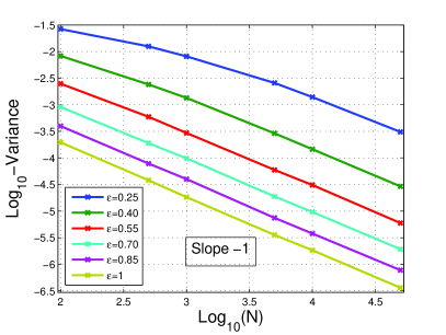
(a) Variance as a function of $N$

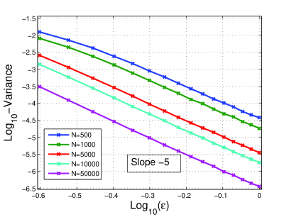
(b) Variance as a function of $\varepsilon$

Figure 1: Variance error as a function of the number of particles, $N$, and the mollifier window width, $\varepsilon$, for dimension $d=5$ at the final time step $T=1$.

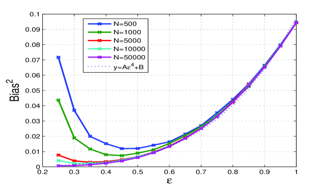
Figure 2: Bias error as a function of the mollifier window width, $\varepsilon$, for dimension $d=5$ at the final time step $T=1$.

9 Appendix

In this appendix, we present the proof of some technical results.

Remark 9.1.

We start with an observation which concerns a possible relaxation of the hypotheses of Lemma 4.3; the uniform convergence assumption for the integrands is crucial and it cannot be replaced by a pointwise convergence.

Let define $\Omega=[0,1]$ equipped with the Borel $\sigma$-field, $(Z_{n})_{n\geq 0}$ a sequence of continuous, real-valued functions s.th.

$$\left\{\begin{array}[]{lll}0&,&x\geq\frac{2}{n}\\ nx&,&x\in[0,\frac{1}{n}]\\ -nx+2&,&x\in[\frac{1}{n},\frac{2}{n}].\end{array}\right.$$ (9.1)

We consider a sequence of probability measures $(m_{n})_{n\geq 0}$ s.th. $m_{n}(dx)=\delta_{\frac{1}{n}}(dx)$ and $m_{0}(dx)=\delta_{0}(dx)$.

On the one hand, we can observe the following.

• $Z_{n}\xrightarrow[\text{$n\rightarrow+\infty$}]{\text{}}0$, pointwise.

• for all $n\geq 0$, $|Z_{n}|\leq 1$, surely.

• $m_{n}\xrightarrow[\text{$n\rightarrow+\infty$}]{\text{}}m$, weakly.

On the other hand,$\int_{0}^{1}Z_{n}dm_{n}=Z_{n}(\frac{1}{n})=1\nrightarrow 0$.

Before stating a tightness criterion for our family of approximating sequences we need to express the classical Theorem of Kolmogorov-Centsov, stated in Theorem 4.10, Chapter 2 in [21], taking into account Remark 4.13.

Proposition 9.2.

Let $r\in\mathbb{N}^{\star}$. A sequence $(\mathbb{P}_{n})_{n\geq 0}$ of Borel probability measures on ${\cal C}^{r}$ is tight if and only if

• $$\lim_{\lambda\longrightarrow+\infty}\;\sup_{n\in\mathbb{N}}\;\mathbb{P}_{n}\left(\left\{\omega\in{\cal C}^{r}\;|\;|\omega_{0}|>\lambda\right\}\right)=0\ ,$$ (9.2)

• $\forall(\varepsilon,s,t)\in\mathbb{R}_{+}^{\star}\times[0,T]\times[0,T]$,

  $$\lim_{\delta\downarrow 0}\;\sup_{n\in\mathbb{N}}\;\mathbb{P}_{n}(\{\omega\in{\cal C}^{r}\;|\;\max_{\underset{|t-s|\leq\delta}{(s,t)\in[0,T]^{2}}}|\omega_{t}-\omega_{s}|>\varepsilon\})=0\ .$$ (9.3)

Lemma 9.3.

Let $K:\mathbb{R}^{d}\rightarrow\mathbb{R}$ be bounded and Lipschitz. For each $n\in\mathbb{N}$, we consider Borel functions $\Phi_{n}:[0,T]\times\mathbb{R}^{d}\times\mathbb{R}\longrightarrow\mathbb{R}^{d\times p}$, $g_{n}:[0,T]\times\mathbb{R}^{d}\times\mathbb{R}\longrightarrow\mathbb{R}^{d}$, and $\Lambda_{n}:[0,T]\times\mathbb{R}^{d}\times\mathbb{R}\longrightarrow\mathbb{R}$ uniformly bounded in $n$. We also consider a tight sequence $(\zeta_{0}^{n})$ of probability measures on $\mathbb{R}^{d}$. Let $(Y^{n},u_{n})$ be solutions of

$$\left\{\begin{array}[]{lll}dY^{n}_{t}=\Phi_{n}(t,Y^{n}_{t},u_{n}(t,Y_{t}^{n}))dW_{t}+g_{n}(t,Y^{n}_{t},u_{n}(t,Y_{t}^{n}))dt\\ u_{n}(t,x):=\int_{\mathcal{C}^{d}}K(x-X_{t}(\omega))\,\exp\left\{\int_{0}^{t}\Lambda_{n}\big{(}r,X_{r}(\omega),u_{n}(r,X_{r}(\omega))\big{)}dr\right\}dm^{n}(\omega)\\ m_{n}={\cal L}(Y_{n}),\end{array}\right.$$ (9.4)

where for all $n\in\mathbb{N}$, $Y^{n}_{0}$ is a r.v. distributed according to $\zeta_{0}^{n}$.
Then, the family $\big{(}\nu^{n}=\mathcal{L}(Y^{n}_{\cdot},u_{n}(\cdot,Y^{n}_{\cdot})),\;n\geq 0\big{)}$ is tight.

Proof.

If we denote by $\mathbb{P}_{n}$ the law of $(Y_{n},u^{n}(\cdot,Y^{n}))$ we bound the l.h.s of (9.2) as follows:

$$\mathbb{P}_{n}(\{\omega\in{\cal C}^{d+1}|\;|\omega_{0}|>\lambda\}) = \mathbb{P}(\{|(Y_{0}^{n},u^{n}(0,Y_{0}^{n}))|>\lambda\})$$ (9.5)

$$\leq \mathbb{P}(\{|Y_{0}^{n}|+|u^{n}(0,Y_{0}^{n})|>\lambda\})$$

$$\leq \mathbb{P}(\{|Y_{0}^{n}|>\frac{\lambda}{2}\})+\mathbb{P}(\{|u^{n}(0,Y_{0}^{n})|>\frac{\lambda}{2}\})$$

$$\leq \zeta^{n}_{0}(\{x\in\mathbb{R}^{d}|\;|x|>\frac{\lambda}{2}\})+\mathbb{P}(\{|u^{n}(0,Y_{0}^{n})|>\frac{\lambda}{2}\}).$$

Let us fix $\varepsilon>0$. On the one hand, $(\zeta^{n}_{0})$ being tight there exists a compact set $\mathfrak{K}_{\varepsilon}$ of $\mathbb{R}^{d}$ such that $\displaystyle{\sup_{n\in\mathbb{N}}\zeta^{n}_{0}(\mathfrak{K}_{\varepsilon}^{c})\leq\varepsilon}$. Then, there exists $\lambda_{\varepsilon}>0$ such that $\{x\in\mathbb{R}^{d}|\;|x|>\frac{\lambda_{\varepsilon}}{2}\}\subset\mathfrak{K}_{\varepsilon}^{c}$ which implies

$${\sup_{n\in\mathbb{N}}\zeta^{n}_{0}(\{x\in\mathbb{R}^{d}|\;|x|>\frac{\lambda_{\varepsilon}}{2}\})\leq\sup_{n\in\mathbb{N}}\zeta^{n}_{0}(\mathfrak{K}_{\varepsilon}^{c})\leq\varepsilon}.$$

On the other hand, since $u^{n}$ is uniformly bounded, for all $\lambda>0$, Chebyshev’s inequality implies

$$\mathbb{P}(\{|u^{n}(0,Y_{0}^{n})|>\frac{\lambda}{2}\})\leq 4\frac{\mathbb{E}[|u^{n}(0,Y^{n}_{0})|^{2}]}{\lambda^{2}}\leq 4\frac{(M_{K}e^{TM_{\Lambda}})^{2}}{\lambda^{2}}\ .$$ (9.6)

Consequently for $\lambda\geq\lambda_{\varepsilon}$, we get

$$\sup_{n\in\mathbb{N}}\mathbb{P}_{n}(\{\omega\in{\cal C}^{d+1}|\;|\omega_{0}|>\lambda\})\leq 4\frac{(M_{K}e^{TM_{\Lambda}})^{2}}{\lambda^{2}}+\varepsilon\ .$$ (9.7)

Taking the limit when $\lambda$ goes to infinity, we finally get inequality (9.2) since $\varepsilon>0$ is arbitrary.

It remains to prove (9.3).
We will make use of Garsia-Rodemich-Rumsey Theorem, see e.g. Theorem 2.1.3, Chapter 2 in [30] or [4]. We will show that, for all $0\leq s<t\leq T$, there exists a positive real constant $C\geq 0$

$$\mathbb{E}{[|Y^{n}_{t}-Y^{n}_{s}|^{4}+|u_{n}(t,Y^{n}_{t})-u_{n}(s,Y^{n}_{s})|^{4}]}\leq C|t-s|^{2}\ ,$$ (9.8)

where $C$ does not depend on $n$. Suppose for a moment that (9.8) holds true.
Let $\varepsilon>0$ fixed. Let $\delta>0$. If $\mathbb{P}_{n}$ denotes again the law of $(Y^{n},u^{n}(\cdot,Y^{n}))$, the quantity

$$\mathbb{P}_{n}(\{\omega\in{\cal C}^{d+1}\;|\;\sup_{\underset{|t-s|\leq\delta}{(s,t)\in[0,T]^{2}}}|\omega_{t}-\omega_{s}|>\varepsilon\})$$ (9.9)

intervening in (9.3) is bounded, up to a constant, by

$$\mathbb{P}(\max_{\underset{|t-s|\leq\delta}{(s,t)\in[0,T]^{2}}}\left\{|Y^{n}_{t}-Y^{n}_{s}|+|u^{n}(t,Y^{n}_{t})-u^{n}(s,Y^{n}_{s})|\right\}>\varepsilon)\ .$$ (9.10)

Let us fix $\gamma\in]0,\frac{1}{4}[$. By Garsia-Rodemich-Rumsey theorem, there is a sequence of non-negative r.v. $\Gamma^{n}$ such that, a.s.

$$\sup_{n\in\mathbb{N}}\mathbb{E}{[(\Gamma^{n})^{4}]}<\infty$$

$$\forall(s,t)\in[0,T]^{2},\;|Y^{n}_{t}-Y^{n}_{s}|+|u^{n}(t,Y^{n}_{t})-u^{n}(s,Y^{n}_{s})|\leq\Gamma^{n}|t-s|^{\gamma}.$$ (9.11)

If $|t-s|\leq\delta$ (9.11) gives

$$\displaystyle{\max_{\underset{|t-s|\leq\delta}{(s,t)\in[0,T]^{2}}}\left\{|Y^{n}_{t}-Y^{n}_{s}|+|u^{n}(t,Y^{n}_{t})-u^{n}(s,Y^{n}_{s})|\right\}\leq\Gamma^{n}\delta^{\gamma}}\ .$$ (9.12)

By (9.12) and Chebyshev’s inequality, for any $n\in\mathbb{N}$, the quantity (9.9) is bounded by

$$\mathbb{P}(\Gamma^{n}\delta^{\gamma}>\varepsilon) = \mathbb{P}(\Gamma^{n}>\varepsilon\delta^{-\gamma})$$

$$\leq \frac{\delta^{4\gamma}}{\varepsilon^{4}},$$

for any $n\in\mathbb{N}$. Since $\delta>0$ is arbitrary, (9.3) follows. To conclude the proof of the lemma, it remains to show (9.8).
We recall that $M_{\Phi}$, $M_{g}$, $M_{\Lambda}$, $M_{K}$ denote the uniform upper bound of the sequences $(|\Phi_{n}|)$, $(|g_{n}|)$, $(|\Lambda_{n}|)$ and of the function $K$. Let $0\leq s<t\leq T$. To show (9.8), we have to evaluate

$$\mathbb{E}{[|Y^{n}_{t}-Y^{n}_{s}|^{4}]}+\mathbb{E}{[|u_{n}(t,Y^{n}_{t})-u_{n}(s,Y^{n}_{s})|^{4}]}\ .$$ (9.13)

By classical computations (e.g. Itô’s isometry, Cauchy-Schwarz inequality), we easily obtain

$$\forall k\in\mathbb{N}^{\star},\;\forall T>0,\;\exists C^{\prime}:=C^{\prime}_{(k,T,M_{\Phi},M_{g},M_{\Lambda})}>0,\;\mathbb{E}{[|Y^{n}_{t}-Y^{n}_{s}|^{2k}]}\leq C^{\prime}|t-s|^{k},$$ (9.14)

where the constant $C^{\prime}$ does not depend on $n$ because $\Phi_{n},g_{n}$ are uniformly bounded, in particular w.r.t. $n$.

Regarding the second expectation in (9.13), we get

$$\mathbb{E}{[|u_{n}(t,Y^{n}_{t})-u_{n}(s,Y^{n}_{s})|^{4}]} = \int_{\mathcal{C}^{d}}\big{(}u_{n}(t,X_{t}(\omega))-u_{n}(s,X_{s}(\omega))\big{)}^{4}dm^{n}(\omega)$$

$$\leq 8(I_{1}+I_{2})\ ,$$

where

$$\begin{array}[]{lll}\displaystyle{I_{1}:=\int_{\mathcal{C}^{d}}\big{(}u_{n}(t,X_{t}(\omega))-u_{n}(s,X_{t}(\omega))\big{)}^{4}dm^{n}(\omega)}\\ \displaystyle{I_{2}:=\int_{\mathcal{C}^{d}}\big{(}u_{n}(s,X_{t}(\omega))-u_{n}(s,X_{s}(\omega))\big{)}^{4}dm^{n}(\omega)\ .}\end{array}$$ (9.16)

On the one hand, for all $x\in\mathbb{R}^{d}$,

$$|u_{n}(t,x)-u_{n}(s,x)| = \Big{|}\mathbb{E}{\Big{[}K(x-Y^{n}_{t})e^{\int_{0}^{t}\Lambda_{n}(r,Y^{n}_{r},u_{n}(r,Y^{n}_{r}))dr}\Big{]}}-\mathbb{E}{\Big{[}K(x-Y^{n}_{s})e^{\int_{0}^{s}\Lambda_{n}(r,Y^{n}_{r},u_{n}(r,Y^{n}_{r}))dr}\Big{]}}\Big{|}$$

$$\leq \int_{\mathcal{C}^{d}}|K(x-X_{t}(\omega))-K(x-X_{s}(\omega))|\exp\left(\int_{0}^{t}\Lambda_{n}(r,X_{r},u_{n}(r,X_{r}))dr\right)dm^{n}(\omega)$$

$$\left.+\;\int_{\mathcal{C}^{d}}K(x-X_{s}(\omega))\;\Big{|}\exp\left(\int_{0}^{t}\Lambda_{n}(r,X_{r}(\omega),u_{n}(r,X_{r}(\omega))\right)dr\right.$$

$$\left.-\;\exp\left(\int_{0}^{s}\Lambda_{n}(r,X_{r}(\omega),u_{n}(r,X_{r}(\omega)))dr\right)\Big{|}\;dm^{n}(\omega)\right.$$

By (2.7) and (9.14) (with $k=1$) together with Cauchy-Schwarz inequality, this is lower than

$$L_{K}\exp(M_{\Lambda}T)\int_{\mathcal{C}^{d}}|X_{t}(\omega)-X_{s}(\omega)|dm^{n}(\omega)$$

$$+ M_{K}\exp(M_{\Lambda})\int_{\mathcal{C}^{d}}\Big{|}\int_{s}^{t}\Lambda_{n}(r,X_{r}(\omega),u_{n}(r,X_{r}(\omega)))dr\Big{|}dm^{n}(\omega)$$

$$\leq (L_{K}\exp(M_{\Lambda}T)\sqrt{C^{\prime}}+M_{K}\exp(M_{\Lambda})M_{\Lambda}\sqrt{T})\sqrt{|t-s|},$$

which implies

$$\begin{array}[]{lll}I_{1}=\int_{\mathcal{C}^{d}}|u_{n}(t,X_{t}(\omega))-u_{n}(s,X_{t}(\omega))|^{4}dm^{n}(\omega)&\leq&(L_{K}\exp(M_{\Lambda}T)\sqrt{C^{\prime}}+M_{K}\exp(M_{\Lambda})M_{\Lambda}\sqrt{T})^{4}|t-s|^{2}\ .\end{array}$$ (9.17)

On the other hand, for all $(x,y)\in\mathbb{R}^{d}\times\mathbb{R}^{d}$

$$\begin{array}[]{lll}|u_{n}(s,x)-u_{n}(s,y)|&\leq&\mathbb{E}{[\big{|}K(x-Y^{n}_{s})-K(y-Y^{n}_{s})\big{|}\exp\big{(}\int_{0}^{s}\Lambda_{n}(r,Y^{n}_{r},u_{n}(r,Y^{n}_{r}))dr\big{)}]}\\ &\leq&L_{K}\exp(M_{\Lambda}T)|x-y|,\ ,\end{array}$$ (9.18)

which implies

$$\begin{array}[]{lll}I_{2}=\int_{\mathcal{C}^{d}}|u_{n}(s,X_{t}(\omega))-u_{n}(s,X_{s}(\omega))|^{4}dm^{n}(\omega)&\leq&L_{K}\exp(M_{\Lambda}T)\int_{\mathcal{C}^{d}}|X_{t}(\omega)-X_{s}(\omega)|^{4}dm^{n}(\omega)\\ &\leq&L_{K}\exp(M_{\Lambda}T)C^{\prime}|t-s|^{2}\ ,\end{array}$$ (9.19)

where the second inequality comes from (9.14) with $k=2$.
Coming back to (9), we have $|I_{1}+I_{2}|\leq C^{\prime\prime}|t-s|^{2}$ with $C^{\prime\prime}$ a constant value depending only on $T,M_{\Phi},M_{g},M_{\Lambda},M_{K},L_{K},T$. This enable us to conclude the proof of (9.8) and finally the one of Lemma 9.3.
∎

We proceed now with the proof of Lemma 8.3, that will make use of the following intermediary result.

Lemma 9.4.

Let $N\in\mathbb{N}^{\star}$. Let $(\xi^{i,N})_{i=1,\cdots,N}$ be a solution of the interacting particle system (7.2); let $(\tilde{\xi}^{i,N})_{i=1,\cdots,N}$ and $\tilde{v}$ as defined as in the discretized interacting particle system (8.1).
Under the same assumptions as in Proposition 8.1, the random variables $V_{t}^{i}:=e^{\int_{0}^{t}\Lambda\big{(}s,\tilde{\xi}^{i,N}_{s},u^{S^{N}(\tilde{\xi})}_{s}(\tilde{\xi}^{i,N}_{s})\big{)}ds}$ and $\tilde{V}_{t}^{i}:=e^{\int_{0}^{t}\Lambda\big{(}r(s),\tilde{\xi}^{i,N}_{r(s)},\tilde{v}_{r(s)}(\tilde{\xi}^{i,N}_{r(s)})\big{)}ds}$, for all $t\in[0,T]$, $i\in\{1,\cdots,N\}$ fulfill the following.

1. For all $t\in[0,T]$, $i\in\{1,\cdots,N\}$

   $$\mathbb{E}[|\tilde{V}_{t}^{i}-V_{t}^{i}|^{2}]\leq C(\delta t)^{2}+C\mathbb{E}\left[\int_{0}^{t}|\tilde{\xi}^{i,N}_{r(s)}-\tilde{\xi}^{i,N}_{s}|^{2}\ ds\right]+C\mathbb{E}\left[\int_{0}^{t}|\tilde{v}_{r(s)}(\tilde{\xi}^{i,N}_{r(s)})-u^{S^{N}(\tilde{\xi})}_{s}(\tilde{\xi}^{i,N}_{s})|^{2}ds\right],$$ (9.20)

   where $C$ is a real positive constant depending only on $M_{\Lambda}$, $L_{\Lambda}$ and $T$.

2. For all $(t,y)\in[0,T]\times\mathbb{R}^{d}$, $i\in\{1,\cdots,N\}$

   $$|\tilde{v}_{t}(y)-u_{t}^{S^{N}(\tilde{\xi})}(y)|^{2}\leq\frac{M_{K}}{N}\sum_{i=1}^{N}K(y-\tilde{\xi}^{i,N}_{t})\;|\tilde{V}_{t}^{i}-V_{t}^{i}|^{2}\ .$$ (9.21)

Proof of Lemma 9.4.

Let us fix $t\in[0,T]$, $i\in\{1,\cdots,N\}$. To prove (9.20), it is enough to recall that $\Lambda$ being uniformly Lipschitz w.r.t. the time and space variables, the inequality (2.7) yields

$$|\tilde{V}_{t}^{i}-V_{t}^{i}|^{2}\leq 3e^{2tM_{\Lambda}}L^{2}_{\Lambda}\int_{0}^{t}\left[|r(s)-s|^{2}+|\tilde{\xi}^{i,N}_{r(s)}-\tilde{\xi}^{i,N}_{s}|^{2}+|\tilde{v}_{r(s)}(\tilde{\xi}^{i,N}_{r(s)})-u_{s}^{S^{N}(\tilde{\xi})}(\tilde{\xi}^{i,N}_{s})|^{2}\right]\,ds\ ,$$ (9.22)

and taking the expectation in both sides of (9.22) implies (9.20) with $C:=3e^{2TM_{\Lambda}}L^{2}_{\Lambda}$.
Let us fix $y\in\mathbb{R}^{d}$. Concerning (9.21), by recalling the third line equation of (8.1) and the linking equation (3.1) (with $m=S^{N}(\tilde{\xi})$), we have

$$|\tilde{v}_{t}(y)-u_{t}^{S^{N}(\tilde{\xi})}(y)|^{2} = \left|\frac{1}{N}\sum_{i=1}^{N}K(y-\tilde{\xi}^{i,N})\tilde{V}^{i}_{t}-\frac{1}{N}\sum_{i=1}^{N}K(y-\tilde{\xi}^{i,N})V^{i}_{t}\right|^{2}$$ (9.23)

$$= \left|\frac{1}{N}\sum_{i=1}^{N}K(y-\tilde{\xi}^{i,N})\left(\tilde{V}^{i}_{t}-V^{i}_{t}\right)\right|^{2}$$

$$\leq \frac{1}{N}\sum_{i=1}^{N}K^{2}(y-\tilde{\xi}^{i,N}_{t})|\tilde{V}_{t}^{i}-V_{t}^{i}|^{2}$$

$$\leq \frac{M_{K}}{N}\sum_{i=1}^{N}K(y-\tilde{\xi}^{i,N}_{t})\;|\tilde{V}_{t}^{i}-V_{t}^{i}|^{2}\ ,$$

which concludes the proof of (9.21) and therefore of Lemma 9.4. ∎

Proof of Lemma 8.3..

All along this proof, $C$ will denote a positive constant that only depends
$T,M_{K},L_{K},M_{\Phi},L_{\Phi},M_{g},L_{g}$ and $M_{\Lambda},L_{\Lambda}$ and that can change from line to line. Let us fix $t\in[0,T]$.

• Inequality (8.4) of Lemma 8.3 is simply a consequence of the fact that the coefficients $\Phi$ and $g$ are uniformly bounded. Indeed,

  $$\mathbb{E}[|\tilde{\xi}^{i,N}_{r(t)}-\tilde{\xi}^{i,N}_{t}|^{2}] = \mathbb{E}\left[\Big{|}\int_{r(t)}^{t}\Phi(\tilde{v}_{r(s)}(\tilde{\xi}^{i,N}_{r(s)}))\,dW_{s}+\int_{r(t)}^{t}g(\tilde{v}_{r(s)}(\tilde{\xi}^{i,N}_{r(s)}))\,ds\Big{|}^{2}\right]$$

  $$\leq 2\mathbb{E}\left[\int_{r(t)}^{t}|\Phi(\tilde{v}_{r(s)}(\tilde{\xi}^{i,N}_{r(s)}))|^{2}\,ds\right]+2(t-r(t))\mathbb{E}\left[\int_{r(t)}^{t}|g(\tilde{v}_{r(s)}(\tilde{\xi}^{i,N}_{r(s)}))|^{2}\,ds\right]$$

  $$\leq 2M^{2}_{\Phi}\delta t+2M^{2}_{g}(\delta t)^{2}$$

  $$\leq C\delta t\ ,\quad\textrm{as soon as }\quad\delta t\in\,]0,1[\ .$$

• Now, let us focus on the second inequality (8.5) of Lemma 8.3. Note that for any $y\in\mathbb{R}^{d}$, the following inequality holds:

  $$|\tilde{v}_{r(t)}(y)-\tilde{v}_{t}(y)| \leq \frac{1}{N}\sum_{i=1}^{N}\left[\left|K(y-\tilde{\xi}^{i,N}_{r(t)})-K(y-\tilde{\xi}^{i,N}_{t})\right|\,e^{\int_{0}^{r(t)}\Lambda\big{(}r(s),\tilde{\xi}^{i,N}_{r(s)},\tilde{v}_{r(s)}(\tilde{\xi}^{i,N}_{r(s)})\big{)}ds}\right.$$

  $$+\left.K(y-\tilde{\xi}^{i,N}_{t})\,\left|e^{\int_{0}^{r(t)}\Lambda\big{(}r(s),\tilde{\xi}^{i,N}_{r(s)},\tilde{v}_{r(s)}(\tilde{\xi}^{i,N}_{r(s)})\big{)}ds}-e^{\int_{0}^{t}\Lambda\big{(}r(s),\tilde{\xi}^{i,N}_{r(s)},\tilde{v}_{r(s)}(\tilde{\xi}^{i,N}_{r(s)})\big{)}ds}\right|\right]\ .$$

  Using the Lipschitz property of $\Lambda$ and the fact that $K$ and $\Lambda$ are bounded, one can apply (2.7) to bound the second term of the sum on the r.h.s. of the above inequality as follows:

  $$K(y-\tilde{\xi}^{i,N}_{t})\,\left|e^{\int_{0}^{r(t)}\Lambda\big{(}r(s),\tilde{\xi}^{i,N}_{r(s)},\tilde{v}_{r(s)}(\tilde{\xi}^{i,N}_{r(s)})\big{)}ds}-e^{\int_{0}^{t}\Lambda\big{(}r(s),\tilde{\xi}^{i,N}_{r(s)},\tilde{v}_{r(s)}(\tilde{\xi}^{i,N}_{r(s)})\big{)}ds}\right| \leq M_{K}e^{(t-r(t))M_{\Lambda}}(t-r(t))M_{\Lambda}$$ (9.25)

  $$\leq C\delta t\ .$$

  The first term of the sum on the r.h.s. of (• ‣ 9) is bounded using the Lipschitz property of $K$ and the fact that $\Lambda$ is bounded.

  $$\left|K(y-\tilde{\xi}^{i,N}_{r(t)})-K(y-\tilde{\xi}^{i,N}_{t})\right|\,e^{\int_{0}^{r(t)}\Lambda\big{(}r(s),\tilde{\xi}^{i,N}_{r(s)},\tilde{v}_{r(s)}(\tilde{\xi}^{i,N}_{r(s)})\big{)}ds}\leq L_{K}e^{tM_{\Lambda}}|\tilde{\xi}^{i,N}_{r(t)}-\tilde{\xi}^{i,N}_{t}|\ .$$ (9.26)

  Injecting (9.25) and (9.26) in (• ‣ 9) we obtain for all $y\in\mathbb{R}^{d}$

  $$|\tilde{v}_{r(t)}(y)-\tilde{v}_{t}(y)|\leq C\delta t+\frac{L_{K}e^{tM_{\Lambda}}}{N}\sum_{i=1}^{N}|\tilde{\xi}^{i,N}_{r(t)}-\tilde{\xi}^{i,N}_{t}|,$$

  which finally implies that

  $$\|\tilde{v}_{r(t)}-\tilde{v}_{t}\|_{\infty}^{2}\leq C\delta t^{2}+\frac{C}{N}\sum_{i=1}^{N}|\tilde{\xi}^{i,N}_{r(t)}-\tilde{\xi}^{i,N}_{t}|^{2}\ .$$

  We conclude by using inequality (8.4) of Lemma 8.3 after taking the expectation of the r.h.s. of the above inequality.

• Finally, we deal with inequality (8.6) of Lemma 8.3. Observe that the error on the left-hand side can be decomposed as

  $$\mathbb{E}[\|\tilde{v}_{r(t)}-u_{t}^{S^{N}(\tilde{\xi})}\|^{2}_{\infty}] \leq 2\mathbb{E}[\|\tilde{v}_{r(t)}-\tilde{v}_{t}\|^{2}_{\infty}]+2\mathbb{E}[\|\tilde{v}_{t}-u_{t}^{S^{N}(\tilde{\xi})}\|^{2}_{\infty}]$$ (9.27)

  $$\leq C\delta t+2\mathbb{E}[\|\tilde{v}_{t}-u_{t}^{S^{N}(\tilde{\xi})}\|^{2}_{\infty}]\ ,$$

  where we have used inequality (8.5) of Lemma 8.3.
  Let us consider the second term on the r.h.s. of the above inequality. To simplify the notations, we introduce the real valued random variables

  $$V_{t}^{i}:=e^{\int_{0}^{t}\Lambda\big{(}s,\tilde{\xi}^{i,N}_{s},u^{S^{N}(\tilde{\xi})}_{s}(\tilde{\xi}^{i,N}_{s})\big{)}ds}\quad\textrm{and}\quad\tilde{V}_{t}^{i}:=e^{\int_{0}^{t}\Lambda\big{(}r(s),\tilde{\xi}^{i,N}_{r(s)},\tilde{v}_{r(s)}(\tilde{\xi}^{i,N}_{r(s)})\big{)}ds}\ ,$$ (9.28)

  defined for any $i=1,\cdots N$ and $t\in[0,T]$.
  Using successively inequalities (9.20) of Lemma 9.4, (8.4) of Lemma 8.3 and (3.5) of Lemma 3.4, we have for all $i\in\{1,\cdots,N\}$,

  $$\mathbb{E}[|\tilde{V}_{t}^{i}-V_{t}^{i}|^{2}] \leq C\delta t+C\mathbb{E}\left[\int_{0}^{t}|\tilde{v}_{r(s)}(\tilde{\xi}^{i,N}_{r(s)})-u^{S^{N}(\tilde{\xi})}_{s}(\tilde{\xi}^{i,N}_{s})|^{2}ds\right]$$ (9.29)

  $$\leq C\delta t+C\mathbb{E}\left[\int_{0}^{t}|\tilde{v}_{r(s)}(\tilde{\xi}^{i,N}_{r(s)})-u^{S^{N}(\tilde{\xi})}_{s}(\tilde{\xi}^{i,N}_{r(s)})|^{2}ds\right]$$

  $$+\;C\mathbb{E}\left[\int_{0}^{t}|u_{s}^{S^{N}(\tilde{\xi})}(\tilde{\xi}^{i,N}_{r(s)})-u^{S^{N}(\tilde{\xi})}_{s}(\tilde{\xi}^{i,N}_{s})|^{2}ds\right]$$

  $$\leq C\delta t+C\int_{0}^{t}\left[\mathbb{E}[\|\tilde{v}_{r(s)}-u^{S^{N}(\tilde{\xi})}_{s}\|_{\infty}^{2}]+\mathbb{E}[|\tilde{\xi}^{i,N}_{r(s)}-\tilde{\xi}^{i,N}_{s}|^{2}]\right]\,ds$$

  $$\leq C\delta t+C\int_{0}^{t}\mathbb{E}[\|\tilde{v}_{r(s)}-u^{S^{N}(\tilde{\xi})}_{s}\|_{\infty}^{2}]\,ds\ .$$

  On the other hand, inequality (9.21) of Lemma 9.4 implies

  $$\|\tilde{v}_{t}-u_{t}^{S^{N}(\tilde{\xi})}\|_{\infty}^{2}\leq\frac{M_{K}^{2}}{N}\sum_{i=1}^{N}|\tilde{V}_{t}^{i}-V_{t}^{i}|^{2}\ .$$ (9.30)

  Taking the expectation in both sides of (9.30) and using (9.29) give

  $$\mathbb{E}[\|\tilde{v}_{t}-u_{t}^{S^{N}(\tilde{\xi})}\|^{2}_{\infty}]\leq\frac{M_{K}^{2}}{N}\sum_{i=1}^{N}\mathbb{E}\left[|\tilde{V}_{t}^{i}-V_{t}^{i}|^{2}\right]\leq C\delta t+C\int_{0}^{t}\mathbb{E}[\|\tilde{v}_{r(s)}-u^{S^{N}(\tilde{\xi})}_{s}\|_{\infty}^{2}]\,ds\ .$$ (9.31)

  We end the proof by injecting this last inequality in (9.27) and by applying Gronwall’s lemma.

∎

ACKNOWLEDGEMENTS. The third named author has benefited partially from the support of the “FMJH Program Gaspard Monge in optimization and operation research” (Project 2014-1607H).

References

- [1] V. Barbu, M. Röckner, and F. Russo. Probabilistic representation for solutions of an irregular porous media type equation: the irregular degenerate case. Probab. Theory Related Fields, 151(1-2):1–43, 2011.
- [2] V. Barbu, M. Röckner, and F. Russo. A stochastic Fokker-Planck equation and double probabilistic representation for the stochastic porous media type equation. arXiv preprint arXiv:1404.5120, 2014.
- [3] G. I. Barenblatt. On some unsteady motions of a liquid and gas in a porous medium. Akad. Nauk SSSR. Prikl. Mat. Meh., 16:67–78, 1952.
- [4] M. T. Barlow and M. Yor. Semimartingale inequalities via the Garsia-Rodemich-Rumsey lemma, and applications to local times. J. Funct. Anal., 49(2):198–229, 1982.
- [5] N. Belaribi, F. Cuvelier, and F. Russo. A probabilistic algorithm approximating solutions of a singular PDE of porous media type. Monte Carlo Methods and Applications, 17(4):317–369, 2011.
- [6] N. Belaribi, F. Cuvelier, and F. Russo. Probabilistic and deterministic algorithms for space multidimensional irregular porous media equation. SPDEs: Analysis and Computations, 1(1):3–62, 2013.
- [7] N. Belaribi and F. Russo. Uniqueness for Fokker-Planck equations with measurable coefficients and applications to the fast diffusion equation. Electron. J. Probab., 17:no. 84, 28, 2012.
- [8] S. Benachour, P. Chassaing, B. Roynette, and P. Vallois. Processus associés à l’équation des milieux poreux. Ann. Scuola Norm. Sup. Pisa Cl. Sci. (4), 23(4):793–832, 1996.
- [9] D. P. Bertsekas and S. E. Shreve. Stochastic optimal control, volume 139 of Mathematics in Science and Engineering. Academic Press, Inc. [Harcourt Brace Jovanovich, Publishers], New York-London, 1978. The discrete time case.
- [10] P. Billingsley. Convergence of probability measures. Wiley Series in Probability and Statistics: Probability and Statistics. John Wiley & Sons, Inc., New York, second edition, 1999. A Wiley-Interscience Publication.
- [11] P. Blanchard, M. Röckner, and F. Russo. Probabilistic representation for solutions of an irregular porous media type equation. Ann. Probab., 38(5):1870–1900, 2010.
- [12] B. Bouchard and N. Touzi. Discrete-time approximation and Monte Carlo simulation of backward stochastic differential equations. Stochastic Process. Appl., 111:175–206, 2004.
- [13] P. Cheridito, H. M. Soner, N. Touzi, and N. Victoir. Second-order backward stochastic differential equations and fully nonlinear parabolic PDEs. Comm. Pure Appl. Math., 60(7):1081–1110, 2007.
- [14] H. Crauel. Random probability measures on Polish spaces, volume 11 of Stochastics Monographs. Taylor & Francis, London, 2002.
- [15] E. B. Dynkin. Superprocesses and partial differential equations. Ann. Probab., 21:1185–1262, 1993.
- [16] W. H. Fleming and H. M. Soner. Controlled Markov processes and viscosity solutions, volume 25 of Stochastic Modelling and Applied Probability. Springer, New York, second edition, 2006.
- [17] E. Gobet, J-P. Lemor, and X. Warin. A regression-based Monte Carlo method to solve backward stochastic differential equations. Ann. Appl. Probab., 15(3):2172–2202, 2005.
- [18] P. Henry-Labordère. Counterparty risk valuation: A marked branching diffusion approach. Available at SSRN: http://ssrn.com/abstract=1995503 or http://dx.doi.org/10.2139/ssrn.1995503, 2012.
- [19] P. Henry-Labordère, X. Tan, and N. Touzi. A numerical algorithm for a class of BSDEs via the branching process. Stochastic Process. Appl., 124(2):1112–1140, 2014.
- [20] B. Jourdain and S. Méléard. Propagation of chaos and fluctuations for a moderate model with smooth initial data. Ann. Inst. H. Poincaré Probab. Statist., 34(6):727–766, 1998.
- [21] I. Karatzas and S. E. Shreve. Brownian motion and stochastic calculus, volume 113 of Graduate Texts in Mathematics. Springer-Verlag, New York, second edition, 1991.
- [22] H. P. Jr. McKean. Propagation of chaos for a class of non-linear parabolic equations. In Stochastic Differential Equations (Lecture Series in Differential Equations, Session 7, Catholic Univ., 1967), pages 41–57. Air Force Office Sci. Res., Arlington, Va., 1967.
- [23] E. Pardoux. Backward stochastic differential equations and viscosity solutions of systems of semilinear parabolic and elliptic PDEs of second order. In Stochastic analysis and related topics, VI (Geilo, 1996), volume 42 of Progr. Probab., pages 79–127. Birkhäuser Boston, Boston, MA, 1998.
- [24] É. Pardoux and S. G. Peng. Adapted solution of a backward stochastic differential equation. Systems Control Lett., 14(1):55–61, 1990.
- [25] E. Pardoux and A. Raşcanu. Stochastic differential equations, Backward SDEs, Partial differential equations, volume 69. Springer, 2014.
- [26] M. Röckner and X. Zhang. Weak uniqueness of Fokker-Planck equations with degenerate and bounded coefficients. C. R. Math. Acad. Sci. Paris, 348(7-8):435–438, 2010.
- [27] L. C. G. Rogers and D. Williams. Diffusions, Markov processes, and martingales. Vol. 1. Cambridge Mathematical Library. Cambridge University Press, Cambridge, 2000. Foundations, Reprint of the second (1994) edition.
- [28] L. C. G. Rogers and D. Williams. Diffusions, Markov processes, and martingales. Vol. 2. Cambridge Mathematical Library. Cambridge University Press, Cambridge, 2000. Itô calculus, Reprint of the second (1994) edition.
- [29] B. W. Silverman. Density estimation for statistics and data analysis. Monographs on Statistics and Applied Probability. Chapman & Hall, London, 1986.
- [30] D. W. Stroock and S. R. S. Varadhan. Multidimensional diffusion processes. Classics in Mathematics. Springer-Verlag, Berlin, 2006. Reprint of the 1997 edition.
- [31] A-S. Sznitman. Topics in propagation of chaos. In École d’Été de Probabilités de Saint-Flour XIX—1989, volume 1464 of Lecture Notes in Math., pages 165–251. Springer, Berlin, 1991.
- [32] C. Villani. Optimal transport, volume 338 of Grundlehren der Mathematischen Wissenschaften [Fundamental Principles of Mathematical Sciences]. Springer-Verlag, Berlin, 2009. Old and new.