Energy Injection in Gamma-ray Burst Afterglows

Abstract

We present multi-wavelength observations and modeling of Gamma-ray Bursts (GRBs) that exhibit a simultaneous re-brightening in their X-ray and optical light curves, and are also detected at radio wavelengths. We show that the re-brightening episodes can be modeled by injection of energy into the blastwave and that in all cases the energy injection rate falls within the theoretical bounds expected for a distribution of energy with ejecta Lorentz factor. Our measured values of the circumburst density, jet opening angle, and beaming corrected kinetic energy are consistent with the distribution of these parameters for long-duration GRBs at both $z\sim 1$ and $z\gtrsim 6$, suggesting that the jet launching mechanism and environment of these events are similar to that of GRBs that do not have bumps in their light curves. However, events exhibiting re-brightening episodes have lower radiative efficiencies than average, suggesting that a majority of the kinetic energy of the outflow is carried by slow-moving ejecta, which is further supported by steep measured distributions of the ejecta energy as a function of Lorentz factor. We do not find evidence for reverse shocks over the energy injection period, implying that the onset of energy injection is a gentle process. We further show that GRBs exhibiting simultaneous X-ray and optical re-brightenings are likely the tail of a distribution of events with varying rates of energy injection, forming the most extreme events in their class. Future X-ray observations of GRB afterglows with Swift and its successors will thus likely discover several more such events, while radio follow-up and multi-wavelength modeling of similar events will unveil the role of energy injection in GRB afterglows.

1. Introduction

Gamma-ray bursts (GRBs) have traditionally been modeled as point explosions that inject $\sim 10^{51}$ erg of energy into a collimated, relativistically-expanding fireball over a period of a few seconds. In this model, the subsequent afterglow radiation is synchrotron emission produced by the interaction of the relativistic ejecta with the circumburst medium. Depending on the density profile of the ambient medium, usually assumed to be either uniform (‘ISM-like’) or falling with radius as $r^{-2}$ (‘wind-like’), this model has several verifiable predictions: smooth light curves at all frequencies from the X-rays to the radio, which rise and fall as the peak of the spectral energy distribution evolves through the observer band; a ‘jet break’ as the expanding ejecta decelerate and begin to spread sideways; and an eventual transition to the sub-relativistic regime where the ejecta become quasi-spherical. In this framework, the energetics of the explosion and the properties of the environment can be determined from fitting light curves with the synchrotron model, while a measurement of the jet break allows for a determination of the angle of collimation of the outflow and the calculation of geometric corrections to the inferred energy.

Despite its simplicity, this model was quite successful in the study of a large number of GRB afterglows (e.g. Berger et al. 2000; Panaitescu & Kumar 2001, 2002; Yost et al. 2003) until the launch of Swift in 2004 (Gehrels et al., 2004). With its rapid-response X-ray and UV/optical afterglow measurements, Swift has revolutionized the study of GRB afterglows. Rapidly-available localizations have allowed detailed ground-based follow-up. X-ray observations from Swift have been even more revolutionary, revealing light curves with multiple breaks falling into a ‘canonical’ series, consisting of a steep decay, plateau, and normal decay, sometimes with evidence for jet-breaks. While the steep decay has been associated with the prompt emission (Tagliaferri et al., 2005; O’Brien et al., 2006) and the normal and post jet-break decay phases are associated with the afterglow, the plateaus cannot be explained by the standard model (Zhang et al. 2006; however, see recent numerical calculations by Duffell & MacFadyen 2014, which suggest that the plateaus may be a natural consequence of a coasting phase in the jet dynamics between $10^{13}$ to $10^{16}$ cm from the progenitor). In addition, short ($\Delta t/t\ll 1$) flares that rise and decline rapidly and exhibit large flux variations ($\Delta F/F\gg 1$; Chincarini et al. 2010; Margutti et al. 2010a) are often seen superposed on the light curves. These flares are believed to be more closely associated with the GRB prompt emission than with the afterglow, and have been interpreted as late-time activity by the central engine (Falcone et al., 2006; Romano et al., 2006; Wang et al., 2006; Pagani et al., 2006; Liang et al., 2006; Lazzati & Perna, 2007; Margutti et al., 2010a; Guidorzi et al., 2015). Some GRBs also exhibit optical flares, which do not always correspond to flares in the X-ray light curves (Li et al., 2012).

These new features of Swift X-ray light curves cannot be simply explained in the traditional picture. New physical mechanisms such as energy injection, circumburst density enhancements, structured jets, viewing angle effects, varying microphysical parameters, and gravitational micro-lensing have been invoked to explain various features of Swift X-ray light curves (Zhang et al., 2006; Nousek et al., 2006; Panaitescu et al., 2006; Toma et al., 2006; Eichler & Granot, 2006; Granot et al., 2006; Jin et al., 2007; Shao & Dai, 2007; Kong et al., 2010; Duffell & MacFadyen, 2014; Uhm & Zhang, 2014). However, although a wealth of information is available from X-ray light curves in general, definitive statements on the physical origin of these features requires synergy with observations at other wavelengths. Ultraviolet (UV), optical, near infra-red (NIR), millimeter, and radio data probe distinct parts of the afterglow spectral energy distribution (SED), and the various physical mechanisms are expected to influence light curves in these bands differently. Thus, a detailed analysis of GRB afterglows requires multi-wavelength data and modeling.

Of the GRBs with plateaus in their X-ray light curves, there is a small class of peculiar events that additionally exhibit an X-ray re-brightening of a non-flaring origin ($\Delta T/T\sim 1$), and an even smaller class where the re-brightening appears to occur simultaneously in both the optical and X-rays (Mangano et al., 2007; Li et al., 2012; Panaitescu et al., 2013). An exemplar of this latter class is GRB 120326A, which exhibits a peak in its well-sampled X-ray light curve at around 0.3 d together with a simultaneous optical re-brightening. Urata et al. (2014) reported optical and millimeter observations of the afterglow of GRB 120326A, and invoked synchrotron self inverse-Compton radiation from a reverse shock to explain the millimeter, optical, and X-ray light curves. By fitting energy-injection models in a wind-like circumburst environment to the X-ray and optical $R$-band light curves, Hou et al. (2014) proposed that a newborn millisecond pulsar with a strong wind was responsible for the re-brightening. Melandri et al. (2014) present multi-band optical and NIR light curves of this event, and explore various physical scenarios for the re-brightening, including the onset of the afterglow, passage of a synchrotron break frequency through the observing band, and geometrical effects.

Here we report detailed radio observations of this event spanning 4 – 220 GHz and 0.3 to 120 d, making this the first GRB with an achromatic re-brightening and with such a rich multi-band data set. We perform the first broad-band modeling for this event using a physical GRB afterglow model (Granot & Sari, 2002) using methods described in Laskar et al. (2013) and Laskar et al. (2014), employing Markov Chain Monte Carlo procedures to characterize the blastwave shock. Our radio observations allow us to constrain the synchrotron self-absorption frequency, and to unambiguously locate the synchrotron peak frequency, together placing strong constraints on the nature of the X-ray/UV/optical re-brightening. We find the clear signature of a jet break at all wavelengths from the radio through the X-rays, allowing us to constrain the true energetics of this event.

We next consider and test various physical processes that may cause a re-brightening in the afterglow light curve, and argue that energy injection is the most plausible mechanism. We model the re-brightening as a power-law increase in blastwave energy, self-consistently accounting for the change in the synchrotron spectrum over the injection period, and compute the fractional increase in energy during the re-brightening. We interpret the energy injection process in the context of a distribution of ejecta Lorentz factors, and provide a measurement of the power law index of the Lorentz factor distribution.

To place our results in context, we search the Swift X-ray light curve archive for all events exhibiting a similar re-brightening, and present full multi-wavelength analyses, complete with deduced correlations between the physical parameters, for all events with radio detections that exhibit simultaneous optical and X-ray re-brightenings. This selection yields three additional events: GRBs 100418A, 100901A, and 120404A. We collect, analyze, and report all X-ray and UV data from the X-ray telescope (XRT) and UV-optical telescope (UVOT) on board Swift for these three events in addition to GRB 120326A. We also analyze and report previously un-published archival radio observations from the Very Large Array (VLA), Submillimeter Array (SMA), and Westerbork Synthesis Radio Telescope (WSRT) for events in our sample, and the first complete multi-wavelength model fits for GRBs 100418A and 100901A. Finally, we compare our results to modeling efforts of a sample of GRBs ranging from $z\sim 1$ to $z\gtrsim 6$, as well as with a complete sample of plateaus in Swift/XRT light curves, and thereby assess the ubiquity of the energy injection phenomenon. We infer the fractional increase in blastwave energy over the plateau phase using simple assumptions on the afterglow properties, and determine the unique characteristics of these events that result in multi-band re-brightenings. We conclude with a discussion of the results from this X-ray-only analysis and our full broad-band modeling in the context of energy injection in GRBs.

Throughout the paper, we use the following values for cosmological parameters: $\Omega_{\rm m}=0.27$, $\Omega_{\rm\Lambda}=0.73$, and $H_{\rm 0}=71\,{\rm km}\,{\rm s}^{-1}\,{\rm Mpc}^{-1}$. All times are in the observer frame, uncertainties are at the 68% confidence level (1$\sigma$), and magnitudes are in the AB system and are not corrected for galactic extinction, unless stated otherwise.

2. GRB Properties and Observations

GRB 120326A was discovered by the Swift Burst Alert Telescope (BAT, Barthelmy et al., 2005) on 2012 March 26 at 01:20:29 UT (Siegel et al., 2012). The burst duration is $T_{90}=26.7\pm 0.4$ s, with a fluence of $F_{\gamma}=(1.1\pm 0.1)\times 10^{-6}$ erg cm^-2 (15–150 keV Barthelmy et al., 2012). A bright X-ray and UV/optical afterglow was detected by Swift (Siegel et al., 2012; Kuin et al., 2012) and numerous ground-based observatories. Spectroscopic observations at the 10.4 m Gran Telescope Canarias (GTC) provided a redshift of $z=1.798$ (Tello et al., 2012).

The burst also triggered the Fermi Gamma-ray Burst Monitor (GBM) at 01:20:31.51 UT (Collazzi, 2012). The burst duration as observed by GBM is $T_{90}=11.8\pm 1.8$ s (50–300 keV) with a fluence of $(3.26\pm 0.05)\times 10^{-6}$ erg cm^-2 (10–1000 keV). The time-averaged $\gamma$-ray spectrum is well fit by a Band function, with break energy, $E_{\rm peak}=43.9\pm 3.9$ keV, low energy index, $\alpha=-0.67\pm 0.19$, and high-energy index, $\beta=-2.33\pm 0.09$ Using the source redshift of $z=1.798$, the inferred isotropic equivalent $\gamma$-ray energy in the 1–$10^{4}$ keV rest frame energy band is $E_{\gamma,\rm iso}=(3.15\pm 0.12)\times 10^{52}$ erg.

2.1. X-ray: Swift/XRT

The Swift X-ray Telescope (XRT, Burrows et al., 2005b) began observing the field at 69 s after the BAT trigger, leading to the detection of an X-ray afterglow. The source was localized to RA = 18h 15m 37.06s, Dec = +69d 15′ 35.4″ (J2000), with an uncertainty radius of 1.4 arcseconds (90% containment). XRT continued observing the afterglow for 18.7 d in photon counting mode, with the last detection at 5.2 d.

We extracted XRT PC-mode spectra using the on-line tool on the Swift website (Evans et al., 2007, 2009) . We analyzed the data after the end of the steep decay at $400$ s using the latest version of the HEASOFT package (v6.14) and corresponding calibration files. We used Xspec (v12.8.1) to fit all available PC-mode data, assuming a photoelectrically absorbed power law model (tbabs $\times$ ztbabs $\times$ pow) and a Galactic neutral hydrogen column density of $N_{\rm H,MW}=6.3\times 10^{20}$ cm^-2 (for consistency with the value used on the Swift website), fixing the source redshift at $z=1.798$. Our best-fit model has a photon index of $\Gamma=1.85\pm 0.04$ and excess absorption corresponding to a neutral hydrogen column (assuming solar metallicity) of $N_{\rm H,{\rm int}}=(4.1\pm 0.7)\times 10^{21}\,{\rm cm}^{-2}$ intrinsic to the host galaxy (C-stat = 497.1 for 570 degrees of freedom). We divided the PC-mode data into 6 roughly equal time bins and extracted time-resolved PC-mode spectra to test for spectral evolution. We do not find clear evidence for significant spectral evolution over this period. In the following analysis, we take the 0.3 – 10 keV count rate light curve from the above website together with $\Gamma_{\rm X}=1.85$ (corresponding to $\beta_{\rm X}\equiv 1-\Gamma_{\rm X}=-0.85$) for the PC mode to compute the 1 keV flux density. We combine the uncertainty in flux calibration based on our spectral analysis (2.7%) in quadrature with the statistical uncertainty from the on-line light curve. For the WT-mode, we convert the count rate light curve to a flux-calibrated light curve using $\Gamma=3.57$ and a count-to-flux conversion factor of $7\times 10^{-11}{\rm erg}\,{\rm cm}^{-2}{\rm ct}^{-1}$ as reported on the on-line spectral analysis.

The WT-mode X-ray light curve declines rapidly as $t^{-3.3\pm 0.1}$. Swift switched to collecting data in PC-mode at 150 s. The PC-mode data between 150 and 300 s continue to decline rapidly as $t^{-3.8\pm 0.4}$, followed by a plateau where the count rate evolves as $t^{-0.22\pm 0.05}$. This part of the lightcurve is likely dominated by the high-latitude prompt emission (Willingale et al., 2010), and we therefore do not consider the rapid decline before 300 s in our afterglow modeling. About 0.16 d after the trigger, the X-ray count rate begins rising and peaks at around 0.41 d. This re-brightening is unusual for X-ray afterglows and we discuss this feature further in section 3.1. The XRT count rate light curve after 1.4 d can be fit by a single power law with a decline rate of $\alpha_{\rm X}=-2.29\pm 0.16$.

Table 1Swift/UVOT Observations of GRB 120326A

$t-t_{0}$	Filter	Frequency	Flux density†	Uncertainty	Detection?
(days)		(Hz)	($\mu$Jy)	($\mu$Jy)	($1=$ Yes)
0.00165	White	8.64e+14	8.89	2.71	1
0.00354	u	8.56e+14	20.7	11.5	0
0.0523	b	6.92e+14	39	6.23	1
0.0546	White	8.64e+14	15.6	2.55	1
0.0558	uvw1	1.16e+15	10.9	3.29	1
0.0582	u	8.56e+14	18.6	4.24	1
0.0594	v	5.55e+14	42.3	14.2	0
0.115	uvw1	1.16e+15	9.16	1.54	1
0.126	u	8.56e+14	30.1	2.34	1
0.134	b	6.92e+14	68.2	8.04	1
0.191	uvw1	1.16e+15	13.8	2.12	1
0.202	u	8.56e+14	50.6	6.19	1
0.258	v	5.55e+14	134	11.8	1
0.285	uvw2	1.48e+15	1.95	0.545	1
0.295	uvm2	1.34e+15	0.607	0.549	0
0.316	v	5.55e+14	150	10.6	1
0.383	uvw1	1.16e+15	19.1	1.94	1
0.393	u	8.56e+14	59.2	3.07	1
0.399	b	6.92e+14	124	13.6	1
0.46	uvw1	1.16e+15	12.3	1.66	1
0.468	u	8.56e+14	43.1	4.43	1
0.527	v	5.55e+14	97.6	9.45	1
0.715	v	5.55e+14	83.9	10.4	1
0.715	uvw1	1.16e+15	11.7	1.35	1
0.737	u	8.56e+14	28.9	4.06	1
0.782	uvw2	1.48e+15	0.968	0.68	0
0.783	b	6.92e+14	50.1	4.38	1
0.792	White	8.64e+14	26.3	3.74	1
1.65	u	8.56e+14	11.6	2.31	1
1.65	uvw2	1.48e+15	0.339	0.668	0
1.66	uvm2	1.34e+15	2.42	1.71	0
1.66	uvw1	1.16e+15	6.29	2.29	0
2.49	uvw1	1.16e+15	3.53	1.67	0
2.49	u	8.56e+14	8.3	1.83	1
2.69	b	6.92e+14	16	4.01	1
2.7	White	8.64e+14	6.59	1.29	1
2.7	v	5.55e+14	31.9	8.93	1
3.72	u	8.56e+14	5.93	1.62	1
3.73	b	6.92e+14	7.59	3.43	0
3.73	uvw1	1.16e+15	0.779	0.626	0
3.73	White	8.64e+14	4.26	0.985	1
3.74	v	5.55e+14	5.94	7.16	0
4.83	u	8.56e+14	2.92	1.42	0
4.83	b	6.92e+14	8.72	3.14	0
4.84	White	8.64e+14	2.06	0.768	0
4.84	v	5.55e+14	5.12	6.37	0
5.73	u	8.56e+14	0.689	1.39	0
5.73	b	6.92e+14	6.41	3.13	0
5.74	White	8.64e+14	0.754	0.719	0
5.74	v	5.55e+14	0.413	6.26	0
17.6	u	8.56e+14	0.28	1.39	0
19.5	u	8.56e+14	2.34	1.28	0

Note. — ^†In cases of non-detections, we report the formal flux density measurement from aperture photometry.

2.2. UV/Optical: Swift/UVOT

The Swift UV/Optical Telescope (UVOT; Roming et al. 2005) observed GRB 120326A using 6 filters spanning the central wavelength range $\lambda_{\rm c}=1928$ Å (W2) to $\lambda_{\rm c}=5468$ Å (v) beginning 67 s after the burst. The afterglow was detected in the initial exposures at RA = 18h 15m 37.13s, Dec = +69d 15′ 35.36″ (J2000) (90% confidence, Kuin et al., 2012), and exhibited a clear re-brightening concomitant with the peak in the X-ray light curve. We analyzed the UVOT data using the latest version of HEASOFT (v. 6.14) and corresponding calibration files. We performed photometry with a $5\arcsec$ aperture and used a $90\arcsec$ annulus with foreground sources masked to estimate the background. We list our derived fluxes in Table 1.

2.3. Optical/NIR: Palomar Observations and GCN Circulars

We observed GRB 120326A with the Wide-Field Infrared Camera (Wilson et al., 2003) on the Palomar 200-inch telescope beginning on 2012 March 30.48 UT. We acquired a series of nine 75 s $J$-band exposures, followed by a series of nine 75 s $K_{s}$-band exposures. We reduced the data following standard IR imaging techniques using a modified version of the WIRCSOFT pipeline and performed aperture photometry of the afterglow in the combined, stacked exposures relative to 2MASS standards in the field.

We also carried out a series of imaging observations of GRB 120326A with the robotic Palomar 60-inch telescope (Cenko et al., 2006) on the nights of 2012 March 31, April 02, April 03 ($r^{\prime}$ and $i^{\prime}$), April 04, April 08, and April 16 ($r^{\prime}$ only). We reduced the images using the P60 automated pipeline and performed aperture photometry relative to secondary standard stars calibrated via separate observations of Landolt (2009) standards.

Finally, we collected other optical and NIR observations of GRB 120326A reported through the Gamma-ray Burst Coordinates Network (GCN) Circulars and converted all photometry to flux densities. We also include the optical photometry of the afterglow published by Melandri et al. (2014) and Urata et al. (2014) in our analysis. We list our complete compilation of optical observations of this burst, together with our P60 and P200 observations, in Table 2.

Table 2Optical Observations of GRB 120326A

$t-t_{0}$	Observatory	Telescope /	Filter	Frequency	Flux density†	Uncertainty	Detection?	Reference
(days)		Instrument		(Hz)	($\mu$Jy)	($\mu$Jy)	($1=$ Yes)
0.000291	TNO	ROTSE	CR	4.56e+14	4.04e+03	1.35e+03	0	Rujopakarn & Flewelling (2012)
0.001	TNO	ROTSE	CR	4.56e+14	926	308	0	Rujopakarn & Flewelling (2012)
0.00189	Calern	TAROT	R	4.56e+14	161	51.2	1	Klotz et al. (2012)
0.00389	Liverpool	RINGO2	R	4.56e+14	120	21.6	1	Melandri et al. (2014)
0.00545	Crni_Vrh	Cicocki	R	4.56e+14	95.1	13.1	1	Melandri et al. (2014)
0.00623	Crni_Vrh	Cicocki	R	4.56e+14	87.6	16.7	1	Melandri et al. (2014)
0.007	Crni_Vrh	Cicocki	R	4.56e+14	86.8	12.9	1	Melandri et al. (2014)
0.00813	Crni_Vrh	Cicocki	R	4.56e+14	74.9	14.3	1	Melandri et al. (2014)
0.00824	Liverpool	RATCam	R	4.56e+14	97.8	17.6	1	Melandri et al. (2014)
0.00968	Crni_Vrh	Cicocki	R	4.56e+14	87.6	14.8	1	Melandri et al. (2014)
0.00991	Liverpool	RATCam	r’	4.81e+14	109	17.2	1	Melandri et al. (2014)
0.0109	Liverpool	RATCam	r’	4.81e+14	91.2	12.6	1	Melandri et al. (2014)
0.0116	Crni_Vrh	Cicocki	R	4.56e+14	82.9	8.84	1	Melandri et al. (2014)
0.0122	Liverpool	SkyCam	R	4.56e+14	90	37.7	1	Melandri et al. (2014)
0.0123	Liverpool	RATCam	r’	4.81e+14	95.5	3.58	1	Melandri et al. (2014)
0.0136	Crni_Vrh	Cicocki	R	4.56e+14	70.2	10.4	1	Melandri et al. (2014)
0.0142	Liverpool	RATCam	i’	3.93e+14	86.3	5.75	1	Melandri et al. (2014)
0.0151	Crni_Vrh	Cicocki	R	4.56e+14	54.8	13.5	1	Melandri et al. (2014)
0.016	Liverpool	RATCam	z’	3.28e+14	111	14.1	1	Melandri et al. (2014)
0.017	Crni_Vrh	Cicocki	R	4.56e+14	49.5	8.92	1	Melandri et al. (2014)
0.0178	Liverpool	RATCam	r’	4.81e+14	72.4	3.41	1	Melandri et al. (2014)
0.0193	Liverpool	RATCam	r’	4.81e+14	67.3	3.82	1	Melandri et al. (2014)
0.0193	Crni_Vrh	Cicocki	R	4.56e+14	54.3	12.2	1	Melandri et al. (2014)
0.0212	Liverpool	RATCam	i’	3.93e+14	68.5	3.89	1	Melandri et al. (2014)
0.0228	Calern	TAROT	R	4.56e+14	70.2	22.3	1	Klotz et al. (2012)
0.0254	Liverpool	RATCam	z’	3.28e+14	103	9.92	1	Melandri et al. (2014)
0.0259	DAO	Skynet	g’	6.29e+14	17.9	5.69	1	Lacluyze et al. (2012)
0.0277	DAO	Skynet	r’	4.56e+14	41	13	1	Lacluyze et al. (2012)
0.028	Liverpool	RATCam	r’	4.81e+14	63.1	3.58	1	Melandri et al. (2014)
0.0296	Liverpool	RATCam	r’	4.81e+14	63.1	2.97	1	Melandri et al. (2014)
0.0311	Liverpool	RATCam	r’	4.81e+14	64.3	3.65	1	Melandri et al. (2014)
0.0333	Liverpool	SkyCam	R	4.56e+14	51.3	43.8	1	Melandri et al. (2014)
0.0344	Liverpool	RATCam	i’	3.93e+14	63.1	4.2	1	Melandri et al. (2014)
0.0358	DAO	Skynet	i’	3.93e+14	73.4	23.4	1	Lacluyze et al. (2012)
0.0396	Liverpool	RATCam	z’	3.28e+14	87.1	8.4	1	Melandri et al. (2014)
0.0709	T17	CDK17	CR	4.56e+14	77	15.6	1	Hentunen et al. (2012)
0.32	LOAO	1m	R	4.56e+14	272	15.4	1	Jang et al. (2012)
0.324	LOAO	1m	R	4.56e+14	298	11.2	1	Jang et al. (2012)
0.327	LOAO	1m	R	4.56e+14	277	10.4	1	Jang et al. (2012)
0.331	LOAO	1m	R	4.56e+14	224	6.28	1	Jang et al. (2012)
0.335	LOAO	1m	R	4.56e+14	212	5.94	1	Jang et al. (2012)
0.338	LOAO	1m	R	4.56e+14	180	5.03	1	Jang et al. (2012)
0.367	McDonald	CQUEAN	r’	4.81e+14	173	2.2	1	Urata et al. (2014)‡
0.371	McDonald	CQUEAN	i’	3.93e+14	181	1	1	Urata et al. (2014)‡
0.375	McDonald	CQUEAN	z’	3.28e+14	233	1.6	1	Urata et al. (2014)‡
0.379	McDonald	CQUEAN	Y’	2.94e+14	264	4	1	Urata et al. (2014)‡
0.383	McDonald	CQUEAN	r’	4.81e+14	164	0.8	1	Urata et al. (2014)‡
0.387	McDonald	CQUEAN	i’	3.93e+14	185	0.5	1	Urata et al. (2014)‡
0.391	McDonald	CQUEAN	z’	3.28e+14	231	2.1	1	Urata et al. (2014)‡
0.398	McDonald	CQUEAN	r’	4.81e+14	151	2.7	1	Urata et al. (2014)‡
0.402	McDonald	CQUEAN	i’	3.93e+14	190	2.3	1	Urata et al. (2014)‡
0.405	McDonald	CQUEAN	z’	3.28e+14	225	7.3	1	Urata et al. (2014)‡
0.418	McDonald	CQUEAN	g’	6.29e+14	115	3.39	1	Urata et al. (2014)‡
0.425	McDonald	CQUEAN	r’	4.81e+14	148	1	1	Urata et al. (2014)‡
0.429	McDonald	CQUEAN	i’	3.93e+14	166	3.9	1	Urata et al. (2014)‡
0.737	GMG	2.4m	R	4.56e+14	101	9.79	1	Zhao et al. (2012)
0.742	GMG	2.4m	v	5.55e+14	148	14.2	1	Zhao et al. (2012)
0.747	Lulin	LOT	i’	3.93e+14	99.1	2.1	1	Urata et al. (2014)‡
0.747	Lulin	LOT	g’	6.29e+14	55.3	0.212	1	Urata et al. (2014)‡
0.75	GMG	2.4m	R	4.56e+14	92.6	8.93	1	Zhao et al. (2012)
0.754	GMG	2.4m	v	5.55e+14	135	13	1	Zhao et al. (2012)
0.758	Lulin	LOT	r’	4.81e+14	85.2	1.11	1	Urata et al. (2014)‡
0.758	Lulin	LOT	z’	3.28e+14	132	8.8	1	Urata et al. (2014)‡
0.794	Lulin	LOT	i’	3.93e+14	98.2	2.8	1	Urata et al. (2014)‡
0.806	Lulin	LOT	z’	3.28e+14	109	8.5	1	Urata et al. (2014)‡
0.81	Xinglong	TNT	R	4.56e+14	115	36.7	1	Xin et al. (2012a)
0.842	Maisoncelles	30cm	R	4.56e+14	111	10.7	1	Sudilovsky et al. (2012)
0.92	BBO	320mm	R	4.56e+14	140	9.33	1	Melandri et al. (2014)
1.36	McDonald	CQUEAN	r’	4.81e+14	49.5	0.36	1	Urata et al. (2014)‡
1.36	McDonald	CQUEAN	i’	3.93e+14	62.9	0.3	1	Urata et al. (2014)‡
1.37	McDonald	CQUEAN	z’	3.28e+14	75.6	0.6	1	Urata et al. (2014)‡
1.37	McDonald	CQUEAN	Y’	2.94e+14	83.4	2.5	1	Urata et al. (2014)‡
1.38	McDonald	CQUEAN	g’	6.29e+14	31	0.72	1	Urata et al. (2014)‡
1.39	LOAO	1m	R	4.56e+14	89.3	15.8	1	Urata et al. (2014)‡
1.43	FLWO	PAIRITEL	K	1.37e+14	248	64.1	1	Melandri et al. (2014)
1.43	FLWO	PAIRITEL	H	1.84e+14	308	137	1	Melandri et al. (2014)
1.43	FLWO	PAIRITEL	J	2.38e+14	121	53.7	1	Melandri et al. (2014)
1.66	Ishigakijima	MITSuME	R	4.56e+14	52.8	4.56	1	Melandri et al. (2014)
1.66	Ishigakijima	MITSuME	g’	6.29e+14	21.3	2.93	1	Melandri et al. (2014)
1.71	Ishigakijima	MITSuME	R	4.56e+14	47.7	4.12	1	Melandri et al. (2014)
1.71	Ishigakijima	MITSuME	g’	6.29e+14	20.5	3.04	1	Melandri et al. (2014)
1.82	Xinglong	TNT	R	4.56e+14	57.3	18.2	1	Xin et al. (2012a)
1.9	Hanle	HCT	R	4.56e+14	41.2	2.74	1	Sahu et al. (2012)
2.01	BBO	320mm	R	4.56e+14	56.8	8.42	1	Melandri et al. (2014)
2.15	Ishigakijima	MITSuME	I	3.93e+14	36.6	7.4	1	Melandri et al. (2014)
2.34	McDonald	CQUEAN	r’	4.81e+14	23.8	3.68	1	Urata et al. (2014)‡
2.35	McDonald	CQUEAN	i’	3.93e+14	33.3	5.34	1	Urata et al. (2014)‡
2.35	McDonald	CQUEAN	z’	3.28e+14	42.7	15.4	1	Urata et al. (2014)‡
2.38	McDonald	CQUEAN	Y’	2.94e+14	59.6	5.4	1	Urata et al. (2014)‡
2.4	LOAO	1m	R	4.56e+14	41.5	7.08	1	Urata et al. (2014)‡
2.4	McDonald	CQUEAN	g’	6.29e+14	18.6	1.81	1	Urata et al. (2014)‡
2.42	FLWO	PAIRITEL	K	1.37e+14	168	43.6	1	Melandri et al. (2014)
2.42	FLWO	PAIRITEL	H	1.84e+14	123	71.8	1	Melandri et al. (2014)
2.42	FLWO	PAIRITEL	J	2.38e+14	43.8	25.6	1	Melandri et al. (2014)
2.43	McDonald	CQUEAN	r’	4.81e+14	26.1	1.3	1	Urata et al. (2014)‡
2.43	McDonald	CQUEAN	i’	3.93e+14	30.5	2.71	1	Urata et al. (2014)‡
2.44	McDonald	CQUEAN	z’	3.28e+14	42.8	5.47	1	Urata et al. (2014)‡
2.6	Ishigakijima	MITSuME	R	4.56e+14	30.6	5.19	1	Melandri et al. (2014)
2.6	Ishigakijima	MITSuME	g’	6.29e+14	14.3	4.91	1	Melandri et al. (2014)
3	BBO	320mm	R	4.56e+14	28	9.24	1	Melandri et al. (2014)
3.32	McDonald	CQUEAN	i’	3.93e+14	21.2	0.864	1	Urata et al. (2014)‡
3.33	McDonald	CQUEAN	z’	3.28e+14	28.1	2.03	1	Urata et al. (2014)‡
3.33	McDonald	CQUEAN	Y’	2.94e+14	44.5	5.3	1	Urata et al. (2014)‡
3.34	McDonald	CQUEAN	r’	4.81e+14	16.8	0.868	1	Urata et al. (2014)‡
3.38	McDonald	CQUEAN	g’	6.29e+14	11.6	1.33	1	Urata et al. (2014)‡
3.43	McDonald	CQUEAN	i’	3.93e+14	21.2	5.02	1	Urata et al. (2014)‡
3.49	LOAO	1m	R	4.56e+14	23	3.74	1	Urata et al. (2014)‡
3.71	Ishigakijima	MITSuME	R	4.56e+14	16.7	2.47	1	Melandri et al. (2014)
3.73	Ishigakijima	MITSuME	g’	6.29e+14	6.31	1.21	1	Melandri et al. (2014)
3.73	Ishigakijima	MITSuME	I	3.93e+14	19.4	4.35	1	Melandri et al. (2014)
3.77	Ishigakijima	MITSuME	R	4.56e+14	16.8	2.32	1	Melandri et al. (2014)
4.4	McDonald	CQUEAN	z’	3.28e+14	13.7	2.3	1	Urata et al. (2014)‡
4.41	McDonald	CQUEAN	i’	3.93e+14	10.8	1.01	1	Urata et al. (2014)‡
4.42	McDonald	CQUEAN	r’	4.81e+14	7.88	0.742	1	Urata et al. (2014)‡
4.43	McDonald	CQUEAN	g’	6.29e+14	5.2	0.32	1	Urata et al. (2014)‡
4.43	Palomar	P200	J	2.38e+14	31.2	3.65	1	This work
4.45	Palomar	P200	K	1.37e+14	33.1	5.97	1	This work
5.25	P60		i’	3.93e+14	6.79	0.519	1	This work
5.26	Palomar	P60	r’	4.81e+14	6.14	0.409	1	This work
5.38	McDonald	CQUEAN	z’	3.28e+14	6.35	3.62	1	Urata et al. (2014)‡
5.39	McDonald	CQUEAN	i’	3.93e+14	6.39	1.06	1	Urata et al. (2014)‡
5.41	McDonald	CQUEAN	r’	4.81e+14	4.65	0.735	1	Urata et al. (2014)‡
5.42	McDonald	CQUEAN	g’	6.29e+14	3.1	0.42	1	Urata et al. (2014)‡
5.92	CRO	51cm	R	4.56e+14	7.56	3.17	1	Melandri et al. (2014)
5.92	CRO	51cm	CR	4.56e+14	5.84	0.563	1	Volnova et al. (2012)
6.4	McDonald	CQUEAN	r’	4.81e+14	2.96	0.0931	1	Urata et al. (2014)‡
6.41	McDonald	CQUEAN	i’	3.93e+14	4.13	0.526	1	Urata et al. (2014)‡
6.42	McDonald	CQUEAN	z’	3.28e+14	5.11	2.44	1	Urata et al. (2014)‡
6.83	LOAO	1m	R	4.56e+14	5.75	0.88	1	Urata et al. (2014)‡
7.24	P60		i’	3.93e+14	6.43	0.885	1	This work
7.25	Palomar	P60	r’	4.81e+14	2.81	0.759	1	This work
7.41	McDonald	CQUEAN	r’	4.81e+14	1.97	0.3	1	Urata et al. (2014)‡
7.51	McDonald	CQUEAN	i’	3.93e+14	2.44	0.29	1	Urata et al. (2014)‡
8.29	P60		i’	3.93e+14	3.37	0.5	1	This work
8.3	Palomar	P60	r’	4.81e+14	2.47	0.392	1	This work
9.29	Palomar	P60	r’	4.81e+14	2.44	0.236	1	This work
13.3	Palomar	P60	r’	4.81e+14	1.98	0.4	1	This work
21.4	Palomar	P60	r’	4.81e+14	1.64	0.11	1	This work

Note. — ^†In cases of non-detections, we report the $3\sigma$ upper limit on the flux density. ^‡ We note that the photometry reported in Table 1 of Urata et al. (2014) yields an unphysical spectral index of $\beta\approx-4.5$. We assume that these numbers have been scaled by the same factors as reported in Figure 4 of their paper, and divide the $gr^{\prime}Rizy$ light curves by a factor of 0.5, 1, 1, 2, 4, and 6, respectively. We further assume that the data have not been corrected for galactic extinction.

2.4. Sub-millimeter: CARMA and SMA

We observed GRB 120326A with the Combined Array for Research in Millimeter Astronomy (CARMA) beginning on 2012 March 30.56 UT (4.52 d after the burst) in continuum wideband mode with $\approx 8$ GHz bandwidth (16 windows, 487.5 MHz each) at a mean frequency of 93 GHz. Following an initial detection (Perley et al., 2012), we obtained two additional epochs. Weather conditions were excellent for each epoch, with the first observation being taken in C configuration (maximum baseline $\sim$370 m), and the following observations in D configuration (maximum baseline $\sim$145 m). For all observations, we utilized 3C371 for bandpass, amplitude and phase gain calibration, and MWC349 for flux calibration. We reduced the data using standard procedures in MIRIAD (Sault et al., 1995). In the last epoch on April 10, we also observed 3C273 and 3C279 and utilized these observations as independent checks on the bandpass and flux calibration. We summarize our observations in Table 3.

The Submillimeter Array (SMA; Ho et al., 2004) observed GRB 120326A at a mean frequency of 222 GHz (1.3 mm; lower sideband centered at 216 GHz, upper sideband at 228 GHz; PI: Urata). Six epochs of observations were obtained between 2012 March 26.43 UT (0.37 d after the burst) and 2012 April 11.64 UT (16.6 d after the burst). These observations have been reported in Urata et al. (2014). We carried out an independent reduction of the data using standard MIR IDL procedures for the SMA, followed by flagging, imaging and analysis in MIRIAD and the Astronomical Image Processing System (AIPS; Greisen, 2003). We utilized 3C279 for bandpass calibration in all but the last epoch, where we utilized J1924-292. We utilized J1800+784 and J1829+487 for gain calibration. We utilized MWC349a for flux calibration, determining a flux density of 1.42 Jy for J1800+784, consistent with flux values in the SMA catalog at similar times. We utilized this flux throughout all observations (not every epoch contained useful flux calibrator scans) and scaled the gains appropriately. We note an uncertainty in the absolute flux density scale of $\approx 15\%$. We detect a source at RA = 18h 15m 37.15s $(\pm 0.02)$ s, Dec = +69d 15′ 35.41″ ($\pm 0.14$; J2000). Two epochs obtained on March 31.40 and April 6.51 showed poor noise characteristics, and we do not include them in our analysis. We measure poorer noise statistics in the observations than reported by Urata et al. (2014), and also do not detect the source in the epoch at 3.53 d, contrary to the previous analysis of this dataset. We report the results of our analysis in Table 3.

2.5. Radio: VLA

We observed the afterglow at C (4–7 GHz), K (18–25 GHz), and Ka (30–38 GHz) bands using the Karl G. Jansky Very Large Array (VLA) starting 5.45 d after the burst. We detected and tracked the flux density of the afterglow over eight epochs until 122 d after the burst, until the source had either faded below or was barely detectable at the $3\sigma$-level at all frequencies. Depending on the start time of the observations, we used either 3C286 or 3C48 as the flux and bandpass calibrator; we used J1806+6949 or J1842+6809 as gain calibrator depending on the array configuration and observing frequency. We carried out data reduction using the Common Astronomy Software Applications (CASA). We list our VLA photometry in Table 3.

Table 3Millimeter and Radio Observations of GRB 120326A

Date	$t-t_{0}$	Observatory∗	Frequency	Integration time	Flux density	Uncertainty†	Detection?
(UT)	(days)		(GHz)	(min)	(mJy)	(mJy)	($1=$ Yes)
2012 Mar 30.56	4.55	CARMA	92.5	60.3	3.38	0.87	1
2012 Apr 5.53	10.51	CARMA	92.5	73.0	1.46	0.42	1
2012 Apr 10.40	15.51	CARMA	92.5	291.9	0.476	0.17	1
2012 Mar 26.43	0.504	SMA‡	222	386	3.3	0.90	1
2012 Mar 27.53	1.55	SMA‡	222	227	2.4	0.80	1
2012 Mar 29.50	3.53	SMA‡	222	252	$<1.8$	0.60	0
2012 Apr 11.64	16.6	SMA‡	222	201	$<2.4$	0.80	0
2012 Mar 31.55	5.66	VLA/C	5.0	8.54	0.674	0.017	1
2012 Mar 31.55	5.66	VLA/C	7.1	4.87	0.369	0.018	1
2012 Mar 31.53	5.64	VLA/C	19.2	9.35	1.25	0.031	1
2012 Mar 31.53	5.64	VLA/C	24.5	7.70	1.49	0.038	1
2012 Apr 04.48	9.42	VLA/C	5.0	5.37	0.411	0.024	1
2012 Apr 04.48	9.42	VLA/C	7.1	6.00	0.561	0.017	1
2012 Apr 04.46	9.41	VLA/C	19.2	7.16	0.825	0.028	1
2012 Apr 04.46	9.40	VLA/C	24.5	8.46	0.936	0.039	1
2012 Apr 04.45	9.40	VLA/C	33.5	7.16	0.94	0.041	1
2012 Apr 10.55	15.49	VLA/C	5.0	7.59	0.313	0.019	1
2012 Apr 10.55	15.49	VLA/C	7.1	6.72	0.352	0.016	1
2012 Apr 10.53	15.48	VLA/C	19.2	7.87	0.667	0.035	1
2012 Apr 10.53	15.48	VLA/C	24.5	7.88	0.686	0.045	1
2012 Apr 10.52	15.46	VLA/C	33.5	7.87	0.706	0.053	1
2012 Apr 26.42	31.37	VLA/C	5.0	5.39	0.409	0.022	1
2012 Apr 26.42	31.37	VLA/C	7.1	4.55	0.562	0.020	1
2012 Apr 26.41	31.35	VLA/C	19.2	13.34	0.458	0.025	1
2012 Apr 26.41	31.35	VLA/C	24.5	9.43	0.401	0.032	1
2012 Apr 26.39	31.34	VLA/C	33.5	7.86	0.277	0.034	1
2012 May 27.49	62.44	VLA/B	5.0	6.11	0.217	0.020	1
2012 May 27.49	62.44	VLA/B	7.1	5.10	0.283	0.017	1
2012 May 27.46	62.40	VLA/B	19.2	20.25	0.183	0.017	1
2012 May 27.46	62.40	VLA/B	24.5	21.98	0.142	0.019	1
2012 Jul 26.17	122.1	VLA/B	5.0	9.81	0.057	0.017	1
2012 Jul 26.17	122.1	VLA/B	7.1	9.77	0.072	0.014	1
2012 Jul 26.12	122.1	VLA/B	19.2	31.85	0.052	0.016	1
2012 Jul 26.12	122.1	VLA/B	24.5	26.57	$<0.07$	0.023	0

Note. — ^∗ The letter following ‘VLA’ indicates the array configuration. ^† $1\sigma$ statistical uncertainties from AIPS task JMFIT (CARMA and SMA observations) or CASA task IMFIT (VLA observations). ^‡PI: Y. Urata.

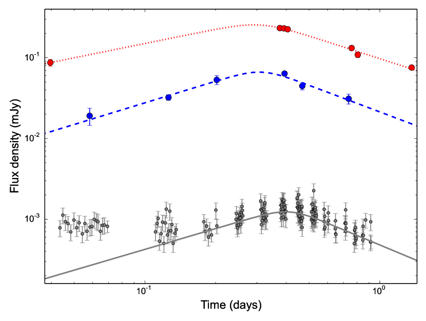
Figure 1.— Broken power law fits to the X-ray (grey, solid), $U$-band (blue, dashed), and $z$-band (red, dotted) light curves for GRB 120326A near the re-brightening around 0.35 d. X-ray points before 0.15 d are not included in the fit. Errorbars at $z$-band are typically smaller than the size of the plotted symbols. The lines correspond to the independent fits at the three frequencies. The best fit parameters are listed in Table 4.

3. Basic Considerations

We consider the X-ray to radio afterglow of GRB 120326A in the context of the standard synchrotron afterglow model, where the afterglow emission is produced by synchrotron radiation from a non-thermal distribution of electrons. The electron energy distribution is assumed to be a power law with electron number density, $n(\gamma)\propto\gamma^{-p},$ for $\gamma>\gamma_{\rm min}$; here $\gamma_{\rm min}$ is the minimum Lorentz factor and the electron energy index, $p$ is expected to lie between 2 and 3. This electron distribution results in a synchrotron spectrum that can be described by a series of power law segments connected at ‘break frequencies’: the self-absorption frequency, $\nu_{\rm a}$, below which synchrotron self-absorption suppresses the flux, the characteristic synchrotron frequency, $\nu_{\rm m}$, which corresponds to emission from electrons with $\gamma=\gamma_{\rm min}$, and the cooling frequency, $\nu_{\rm c}$, above which synchrotron cooling is important; the flux density at $\nu_{\rm m}$ sets the overall flux normalization. The synchrotron model is described in detail in Sari et al. (1998), Chevalier & Li (2000) and Granot & Sari (2002).

3.1. X-ray/UV/Optical Re-brightening at 0.4 d

A prominent feature of the afterglow light curve of GRB 120326A is a re-brightening at about 0.4 d. We quantify the shape of the light curve at the re-brightening by fitting the X-ray data with a smoothly-joined broken power law of the form

$$F_{\nu}=F_{\rm b}\left(\frac{(t/t_{\rm b})^{-y\alpha_{1}}+(t/t_{\rm b})^{-y\alpha_{2}}}{2}\right)^{-1/y},$$ (1)

where $t_{\rm b}$ is the break time, $F_{\rm b}$ is the flux at the break time, $\alpha_{1}$ and $\alpha_{2}$ are the temporal indices before and after the break, respectively, and $y$ is the sharpness of the break . The X-ray data before 0.15 d exhibit a plateau and we therefore restrict the fit to span 0.15 to 1.25 d. We use the Python function curve_fit to estimate these model parameters and the associated covariance matrix. Our best-fit parameters are $t_{\rm b}=(0.41\pm 0.02)\,\rm{d}$, $\alpha_{1}=0.85\pm 0.19$, $\alpha_{2}=-1.22\pm 0.18$, and $y=5\pm 4$ (Figure 1 and Table 4).

The optical data are more sparsely sampled than the X-ray observations. We fit the $U$-band data between 0.05 d and 1.25 d after fixing $y=5$ as suggested by the fit to the better-sampled X-ray light curve. Our derived value of the peak time, $t_{\rm b}=0.31\pm 0.04$ is marginally earlier than, but close to the peak time of the X-ray light curve. The rise and decay rate in $U$-band are also statistically consistent with those derived from the X-ray light curve. Similarly, we fit the $z$-band light curve between 0.04 d and 1.4 d, fixing $y=5$. Since this time range includes a single point prior to the peak, the peak time and rise rate are degenerate in the fit. We therefore fix $t_{\rm b}=0.31$ as derived from the $U$-band fit. The best-fit parameters are listed in Table 4, and are consistent with those derived for the UV and X-ray light curves.

Finally, we fit the X-ray, UV, and interpolated optical/NIR data jointly, where the three light curves are constrained to the same rise and decay rate, time of peak, and sharpness of the break, with independent normalizations in the three bands. Using a Markov Chain Monte Carlo simulation using emcee (Foreman-Mackey et al., 2013), we find $t_{\rm b}=0.40\pm 0.01$, $\alpha_{1}=0.52\pm 0.06$, and $\alpha_{2}=-1.10\pm 0.10$.

In summary, the X-ray/UV/optical light curves exhibit a prominent peak, nearly simultaneously in multiple bands (X-rays through the optical), which, therefore, cannot be related to the passage of a synchrotron break frequency. We explore various explanations for this behavior in Section 5.2.4.

3.2. X-ray/radio Steep Decline: $\nu_{\rm m}$ and $t_{\rm jet}$

The X-ray data at $\gtrsim 1.4\,$d exhibit a steep decline, with $\alpha_{\rm X}=-2.29\pm 0.16$. In the standard afterglow model a steep decline of $\alpha\approx-p\lesssim-2$ at frequencies above $\nu_{\rm m}$ is expected after the ‘jet-break’ ($t_{\rm jet}$), when the bulk Lorentz factor, $\Gamma$, decreases below the inverse opening angle of the jet, $1/\theta_{\rm jet}$, and the edges of the collimated outflow become visible. The $r^{\prime}$-band light curve also exhibits a shallow-to-steep transition at $\approx 1.5$ d, with a post-break decay rate of $\alpha_{\rm R}=-2.27\pm 0.11$, consistent with the X-rays. These observations suggest that the jet break occurs at about $1.5$ d. We now consider whether this interpretation is consistent with the radio observations.

The multi-wavelength radio SED at 9 d is well-fit by a single power law with spectral index, $\beta=\nicefrac{{1}}{{3}}$ from 7 GHz to 93 GHz (Figure 2 and Section 3.4), indicating that $\nu_{\rm m}>93$ GHz at this time. In the absence of a jet break, we would expect the flux density below $\nu_{\rm m}$ to remain constant (for a wind-like circumburst environment) or rise with time (for a constant density circumburst environment). However, the radio light curves decline after 4.6 d at all frequencies from 15 GHz to 93 GHz. The combination of $\nu_{\rm m}>93$ GHz at 9 d and the declining light curve in the radio bands is only possible in the standard afterglow model if a jet break has occurred before 4.6 d. This is consistent with the steepening observed in the X-ray and optical light curves at $\approx 1.5$ d, suggesting that $t_{\rm jet}\approx 1.5$ d.

We note that the flux at a given frequency decays steeply following a jet break only once $\nu_{\rm m}$ has crossed the observing frequency; thus the steepening in the radio light curves is expected to be delayed past that of the steepening in the X-ray and optical light curves until $\nu_{\rm m}$ passes through the radio band. We find that the 7 GHz light curve is consistent with being flat to 50 d, after which it declines rapidly with $\alpha_{\rm radio}\approx-2$. This suggests that $\nu_{\rm m}$ crosses the $7$ GHz band at around $50$ d. Since $\nu_{\rm m}$ is expected to decline as $t^{-2}$ following the jet break, we have $\nu_{\rm m}\approx 8\times 10^{12}$ Hz at 1.5 d if we take $t_{\rm jet}\approx 1.5$ days. Thus $\nu_{\rm m}$ is below both the X-rays and the optical frequencies at $t=t_{\rm jet}$, consistent with the steepening being observed around the same time in the X-ray and optical bands.

To summarize, a simultaneous steepening in the X-ray and optical light curves between 1 and 2 d indicates that $t_{\rm jet}\approx 1.5$ d. Taken together with a similar steepening observed in the 7 GHz radio light curve around 50 d, we find $\nu_{\rm m}\approx 7$ GHz at 50 d.

Table 4Parameters for broken power law fit to X-ray/UV/optical re-brightening for GRB 120326A

	XRT	$U$-band	$z$-band	Joint‡ (MCMC)
Break time, $t_{\rm b}$ (d)	$0.41\pm 0.02$	$0.31\pm 0.04$	$0.31^{{\dagger}}$	$0.40\pm 0.02$
Flux density at $t_{\rm b}$, $F_{\rm b}$ ($\mu$Jy)	$1.23\pm 0.05$	$66\pm 7$	$255\pm 10$	—
Rise rate, $\alpha_{1}$	$0.85\pm 0.19$	$0.89\pm 0.21$	$0.59\pm 0.03$	$0.52\pm 0.06$
Decay rate, $\alpha_{2}$	$-1.22\pm 0.18$	$-1.10\pm 0.29$	$-0.94\pm 0.05$	$-1.10\pm 0.10$
Smoothness, $y$	$5.0\pm 4.0$	$5.0^{{\dagger}}$	$5.0^{{\dagger}}$	$17\pm 10$

Note. — ^† Parameters fixed during fit (see text for details). ^‡ We used a flat prior on all parameters, with the ranges $t_{\rm b}\in[0.05,1.0]$, $F_{\rm b,X}\in[1\times 10^{-4},1\times 10^{-2}]$ mJy, $F_{\rm b,UV}\in[5\times 10^{-3},1\times 10^{-1}]$ mJy, $F_{\rm b,z}\in[1\times 10^{-2},2]$ mJy,$\alpha_{1}\in[0.1,5.0]$,$\alpha_{2}\in[-5.0,0.0]$, and $y\in[0.5,30]$.

3.3. The Circumburst Density Profile and the Location of $\nu_{\rm c}$

The density profile in the immediate (sub-pc scale) environment of the GRB progenitor impacts the hydrodynamic evolution of the shock powering the GRB afterglow. The evolution of the shock Lorentz factor is directly reflected in the afterglow light curves at all frequencies and multi-band modeling of GRB afterglows therefore allows us to disentangle different density profiles. Since the progenitors of long-duration GRBs are believed to be massive stars, the circumburst density structure is expected to be shaped by the stellar wind of the progenitor into a profile that falls of as $\rho(r)=Ar^{-2}$ with radius $r$. Here $A={\dot{M}_{w}}/4\pi V_{w}\equiv 5\times 10^{11}A_{*}$ g cm^-1 is a constant proportional to the progenitor mass-loss rate $\dot{M}_{w}$ (assumed constant), for a given wind speed, $V_{w}$ (Chevalier & Li, 2000), and $A_{*}$ is a dimensionless parametrization, corresponding to $\dot{M}_{w}=1\times 10^{-5}\,M_{\odot}\,{\rm yr}^{-1}$ and $V_{w}=1000$ km s^-1. Alternatively, the shock may directly encounter the uniform interstellar medium (ISM). Both wind- and ISM-like environments have been inferred for different events from previous observations of GRB afterglows (e.g., Panaitescu & Kumar 2000; Harrison et al. 2001; Panaitescu & Kumar 2001, 2002; Yost et al. 2002; Frail et al. 2003; Chandra et al. 2008; Cenko et al. 2010, 2011; Laskar et al. 2013, 2014). Here, we explore the constraints on the progenitor environment of GRB 120326A.

The spectral index between the PAIRITEL $K$-band observation at 1.4 d (Morgan, 2012) and the X-rays is $\beta_{\rm NIR,X}=-0.96\pm 0.05$ (Figure 3), which is consistent with the X-ray spectral index of $\beta_{\rm X}=-0.85\pm 0.04$ (Section 2.1) at $2\sigma$, suggesting that the NIR, optical, and X-ray bands are located on the same power law segment of the afterglow SED at 1.4 d. At the same time, the spectral index within the NIR/optical bands is $\beta=-1.80\pm 0.16$, indicating that extinction is present.

Since $\beta_{\rm NIR,X}\approx\beta_{\rm X}\approx-0.90$, the cooling frequency, $\nu_{\rm c}$ must lie either below the NIR or above the X-rays at 1.4 d. For $\nu_{\rm c}<\nu_{\rm IR}$, we would infer an electron energy index, $p\approx 1.8$ and a light curve decay rate of $\alpha\approx-0.85$ regardless of the circumburst density profile. On the other hand, $\nu_{\rm c}>\nu_{\rm X}$ requires $p\approx 2.8$ with $\alpha\approx-1.35$ for a constant density environment and $\alpha\approx-1.85$ for a wind-like environment. Actual measurements of the light curve decay rate at $\approx 1.4$ d are complicated by the presence of the jet break at around this time. The optical and X-ray light curves decline as $\alpha_{\rm R}=-2.05\pm 0.13$ and $\alpha_{\rm X}=2.29\pm 0.16$ after the jet break, with the expected decay rate being $\alpha\approx-p$ (Rhoads, 1999; Sari et al., 1999). This indicates $p\approx 2$ (Section 3.2) and $\nu_{\rm c}<\nu_{\rm m}$ for an ISM model. Upon detailed investigation (Section 4), we find that a $p\approx 2$ model with an ISM-like environment fits the data after the re-brightening well. This model additionally requires $\nu_{\rm c}<\nu_{\rm m}$ (fast cooling) until $\approx 2$ d. For completeness, we present our investigation of the wind model in Appendix B.

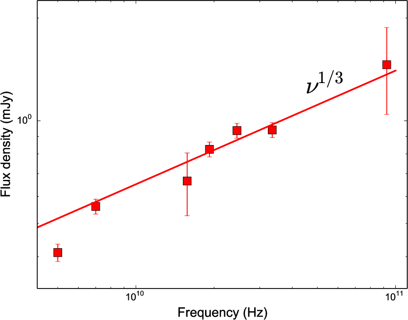
Figure 2.— Afterglow SED for GRB 120326A at 9 d from 5 GHz to 92.5 GHz together with a best fit power law fit to the data above 7 GHz. The spectrum is optically thin with a spectral index of $\nu^{0.35\pm 0.03}$ from 7 GHz to 92.5 GHz. The 5 GHz observation shows evidence of synchrotron self-absorption.

Figure 3.— Afterglow SED for GRB 120326A at 0.33 d from the NIR to the X-rays together with the best fit forward shock model (red, solid). The optical and UV data exhibit a clear decrement due to extinction in the host galaxy. The solid line is the SED from the highest-likelihood model and the dashed curve indicates the SED in the absence of absorption along the line of sight to the GRB by the Milky Way and the GRB host (Section 5.1). The spectral break apparent in the model SED at $\approx 10^{14}$ Hz is $\nu_{\rm m}$. The data above $\approx 9\times 10^{14}$ Hz (Ly-$\alpha$ in GRB rest frame) are likely affected by absorption by the intergalactic medium (IGM) along the line of sight.

3.4. Location of $\nu_{\rm a}$

The radio SED from 7 GHz to 93 GHz at $\approx 9$ days is optically thin with a spectral slope of $\beta=0.33\pm 0.04$ (Figure 2), suggesting that $\nu_{\rm m}$ lies above 93 GHz and $\nu_{\rm a}$ lies below 7 GHz at this time. This is consistent with the passage of $\nu_{\rm m}$ through 7 GHz at 50 d inferred in Section 3.2. The spectral index between 5 GHz and 7 GHz at 9 d, $\beta=0.92\pm 0.23$, is steeper than $\nu^{1/3}$. This may suggest that the synchrotron self-absorption frequency, $\nu_{\rm a}\approx 5$ GHz. However, this spectral index does not show a monotonic trend with time. Since this part of the radio spectrum is strongly affected by interstellar scintillation (ISS) in the ISM of the Milky Way, a unique interpretation of the observed spectral index is difficult at these frequencies. This difficulty in constraining $\nu_{\rm a}$ results in degeneracies in the physical parameters. We return to this point in Section 5.1.

4. Multi-wavelength Modeling

Although the panchromatic peak at 0.4 d is a unique feature of GRB 120326A, the X-ray, optical, and radio light curves of this event exhibits standard afterglow features after this time, with evidence for an un-broken power law spectrum extending from the optical to the X-rays (Section 3.3), a $\nu^{\nicefrac{{1}}{{3}}}$ spectrum in the radio (Section 3.4), and evidence for a jet break at $t_{\rm jet}\approx 1.5$ d. (Section 3.2). We therefore determine the physical properties of this event by using observations after the X-ray/optical peak. We model the data at $\gtrsim 0.4$ d as arising from the afterglow blastwave, using the smoothly-connected power law synchrotron spectra described by Granot & Sari (2002). We compute the break frequencies and normalizations using the standard parameters: the fractions of the blastwave energy imparted to relativistic electrons ($\epsilon_{\rm e}$) and magnetic fields ($\epsilon_{B}$), the kinetic energy ($E_{\rm K,iso}$), and the circumburst density ($n_{0}$). We also use the SMC extinction curve (Pei, 1992) to model the extinction in the host galaxy ($A_{\rm V}$). Since the $R$-band light curve flattens at $\approx 10$ days due to contribution from the host, we fit for the $R$-band flux density of the host galaxy as an additional free parameter.

The various possible orderings of the spectral break frequencies (e.g., $\nu_{\rm m}<\nu_{\rm c}$: ‘slow cooling’ and $\nu_{\rm c}<\nu_{\rm m}$: ‘fast cooling’) give rise to five possible shapes of the afterglow SED (Granot & Sari, 2002). Due to the hydrodynamics of the blastwave, the break frequencies evolve with time and the SED transitions between spectral shapes. To preserve smooth light curves when break frequencies cross and the spectral shape changes, we employ the weighting schemes described in Laskar et al. (2014) to compute the afterglow SED as a function of time. To efficiently and rapidly sample the available parameter space, we carry out a Markov Chain Monte Carlo (MCMC) analysis using a python implementation of the ensemble MCMC sampler emcee (Foreman-Mackey et al., 2013). For a detailed discussion of our modeling scheme, see Laskar et al. (2014). To account for heterogeneity of UV/Optical/NIR data collected from different observatories, we usually impose an uncertainty floor of $5\%$ prior to fitting with our modeling software. For this GRB, we find that the fit is driven by the optical data at the expense of fits at the radio and X-ray bands, which we mitigate by increasing the uncertainty floor further to $12\%$. We additionally correct for the effect of inverse Compton cooling (Appendix A).

5. Results for GRB 120326A

5.1. Multi-wavelength model at $\gtrsim 0.4$ d

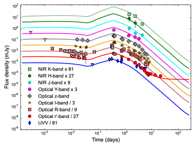
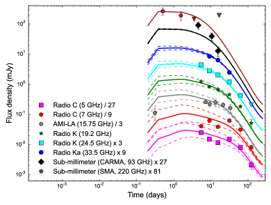
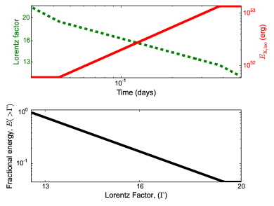
Figure 4.— X-ray, UV (top left), optical (top right), and radio (bottom left) light curves of GRB 120326A in the ISM scenario, with the full afterglow model (solid lines), including energy injection before 0.4 d. The X-ray data before 0.004 d is likely dominated by high-latitude prompt emission and we do not include these data in our analysis. The dashed envelopes around the radio light curves indicate the expected effect of scintillation at the $1\sigma$ level. The data prior to the end of the re-brightening at 0.4 d (open symbols) are not used to determine the parameters of the forward shock in the MCMC analysis. The Swift/UVOT data in the uvw2 and uvm2 bands are strongly affected by IGM absorption and are not included in the analysis. Bottom right: blastwave Lorentz factor (green, dashed; upper sub-panel) and isotropic equivalent kinetic energy (red, solid; upper sub-panel) as a function of time, together with the energy distribution across ejecta Lorentz factors (black, solid; lower sub-panel) as determined from fitting the X-ray/UV/optical re-brightening at 0.4 d.

In confirmation of the basic analysis presented in Section 3.3, our highest likelihood model (Figure 4) has $p\approx 2.09$, $\epsilon_{\rm e}\approx 0.33$, $\epsilon_{B}\approx 0.33$, $n_{0}\approx 0.27\,{\rm cm}^{-3}$, $E_{\rm K,iso}\approx 1.4\times 10^{53}$ erg, $t_{\rm jet}\approx 1.5$ d, $A_{\rm V}\approx 0.48$ mag, and an $r^{\prime}$-band flux density of $2.3\,\mu$Jy for the host galaxy. The spectrum is in fast cooling until 1.4 d. During the fast cooling phase, $\nu_{\rm a}$ splits into two distinct frequencies: $\nu_{\rm ac}$ and $\nu_{\rm sa}$ (Granot & Sari, 2002). The spectrum has the Rayleigh-Jeans shape ($\nu^{2}$) below $\nu_{\rm ac}$, and a slope of $\nu^{11/8}$ between $\nu_{\rm ac}$ and $\nu_{\rm sa}$. For the highest likelihood model, the break frequencies are located at $\nu_{\rm ac}\approx 2.8\times 10^{9}$ Hz, $\nu_{\rm sa}\approx 4.9\times 10^{9}$ Hz, $\nu_{\rm c}\approx 9.3\times 10^{12}$, and $\nu_{\rm m}\approx 1.5\times 10^{13}$ Hz at 1 d and the peak flux density is $\approx 18$ mJy at $\nu_{\rm c}$. $\nu_{\rm m}$ evolves as $t^{-2}$ following the jet break at $\approx 1.5$ d to $\approx 7.7$ GHz at 50 d, consistent with the basic considerations outlined in Section 3.2. The Compton $y$-parameter is $\approx 0.6$, indicating that cooling due to inverse-Compton scattering is moderately significant.

We present histograms of the marginalized posterior density for each parameter in Figure 5. Most of our radio observations are after the transition to slow cooling, at which time $\nu_{\rm a}$ lies below the lowest radio frequency observed, resulting in degeneracies between the model parameters (Figure 6). We summarize the results of our MCMC analysis in Table 5.

Using the relation

$$\theta_{\rm jet}=0.17\left(\frac{E_{\rm K,iso,52}}{n_{0}}\right)^{\frac{1}{8}}\left(\frac{t_{\rm jet}/(1+z)}{1\,\rm d}\right)^{\frac{3}{8}}$$ (2)

for the jet opening angle (Sari et al., 1999), and the distributions of $E_{\rm K,iso}$, $n_{0}$, and $t_{\rm jet}$ from our MCMC simulations, we find $\theta_{\rm jet}=4.6\pm 0.2$ degrees. Applying the beaming correction, $E=E_{\rm iso}(1-\cos{\theta_{\rm jet}})$, we find $E_{\gamma}=(1.0\pm 0.1)\times 10^{50}$ erg (1–$10^{4}$ keV; rest frame) and $E_{\rm K}=\left(4.6^{+0.2}_{-0.1}\right)\times 10^{50}$ erg.

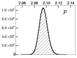
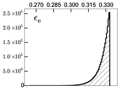
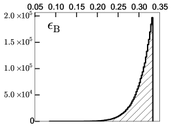
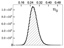
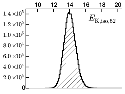
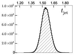
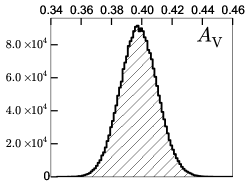
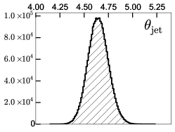
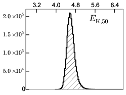
Figure 5.— Posterior probability density functions for the physical parameters of GRB 120326A in the ISM model from MCMC simulations. We have restricted $\epsilon_{\rm e}<\nicefrac{{1}}{{3}}$ and $\epsilon_{\rm B}<\nicefrac{{1}}{{3}}$.

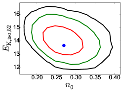
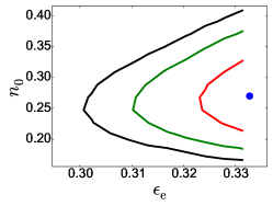
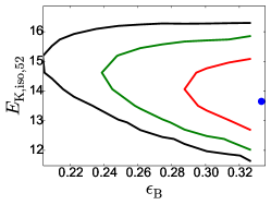
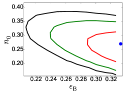
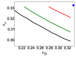
Figure 6.— 1$\sigma$ (red), 2$\sigma$ (green), and 3$\sigma$ (black) contours for correlations between the physical parameters, $E_{\rm K,iso}$, $n_{0}$, $\epsilon_{\rm e}$, and $\epsilon_{B}$ for GRB 120326A, in the ISM model from Markov chain Monte Carlo simulations, together with the maximum-likelihood model (blue dot). We have restricted $\epsilon_{\rm e}<\nicefrac{{1}}{{3}}$ and $\epsilon_{\rm B}<\nicefrac{{1}}{{3}}$. See the on-line version of this Figure for additional plots of correlations between these parameters and $p$, $t_{\rm jet}$, $\theta_{\rm jet}$, $E_{\rm K}$, $A_{\rm V}$, and $F_{\nu,{\rm host,R}}$.

5.2. X-ray/UV/optical Re-brightening

We now consider physical explanations of the unusual re-brightening between 0.1 and 1 day observed in the X-ray, UV, and optical bands.

Scattering by dust grains in the host galaxy of GRBs has been suggested as a potential explanation for the shallow decay phase of X-ray light curves (Shao & Dai, 2007). However, this mechanism is expected to cause a significant softening of the X-ray spectrum with time (Shen et al., 2008), and cannot produce light curves that rise with time, as is observed in the case of GRB 120326A at about 0.4 d. The bump can also not be caused by the passage of a spectral break frequency, since it occurs almost simultaneously in the X-ray, UV, and optical bands. Four remaining potential models for the bump are: (1) onset of the afterglow, (2) geometric effects due to an observer located outside the jet (off-axis scenario), (3) a density enhancement in the circumburst environment, and (4) a refreshed shock (energy injection scenario). We now explore these possibilities in turn.

5.2.1 Afterglow onset

In this scenario, the peak of the light curve emission corresponds to emission from a reverse shock due to deceleration of the ejecta by the surrounding material. The ejecta are assumed to be composed of a conical shell segment at a single Lorentz factor. The reverse shock light curves before and after the deceleration time depend on the properties of the environment (ISM or wind) and the ejecta. Reverse shock light curves for a constant density environment depend upon whether the ejecta shell is thick ($\Delta_{0}>l/2\Gamma_{0}^{\nicefrac{{8}}{{3}}}$) or thin ($\Delta_{0}>l/2\Gamma_{0}^{\nicefrac{{8}}{{3}}}$), where $\Delta_{0}$ is the initial shell width, $\Gamma_{0}$ is the initial Lorentz factor of the ejecta and $l=(3E/4\pi n_{0}m_{\rm p}c^{2})^{1/3}$ is the Sedov length (Kobayashi, 2000). Similarly, when the circumburst medium has a wind-like profile, the light curves again depend on whether $\Delta_{0}>E/4\pi Ac^{2}\Gamma_{0}^{4}$ (thick shell) or $\Delta_{0}<E/4\pi Ac^{2}\Gamma_{0}^{4}$ (thin shell; Kobayashi & Zhang 2003).

In the thick shell case, the reverse shock crosses the ejecta in a time comparable to the burst duration, $t_{\gamma}$, and the light curves at all frequencies are expected to peak at that time scale. In the case of GRB 120326A, $T_{90}$ in the Swift/BAT band is $\approx 27$ s, which is much shorter than the observed time at which the light curves peak, $t_{\rm peak}\approx 0.4$ d. Thus, the re-brightening cannot be explained by reverse shock emission in the thick shell case.

In the thin shell case, temporal separation is expected between the GRB itself and the peak of the reverse shock, which occurs when the RS crosses the shell at $t_{\gamma}=90E_{\rm K,iso,52}^{1/3}n_{0}^{-1/3}\Gamma_{0,100}^{-8/3}$ s (ISM environment; Kobayashi 2000) or $t=2.9\times 10^{3}(1+z)E_{\rm K,iso,52}\Gamma_{0,100}^{-4}A_{*}^{-1}$ s (wind environment; Zou et al. 2005). A reverse shock peak at $0.4$ d would imply a rather low burst Lorentz factor of $\Gamma_{0}\approx 17$. Additionally, the light curves at all frequencies would be expected to rise until $t_{\gamma}$ and decline thereafter (except above $\nu_{\rm c}$ where the flux is constant until $t_{\gamma}$ and disappears after $t_{\gamma}$). The observed $R$-band light curve, on the other hand, declines between $100$ s and $500$ s, followed by a flat segment until $3500$ s, followed by the rise into the bump at $0.4$ d. This combination of a flat portion followed by a rise cannot be explained as being due to a reverse shock.

Thus the onset of the afterglow does not provide a viable explanation for the re-brightening regardless of density profile, and whether the ejecta are in the thick- or thin-shell regime.

5.2.2 Off-axis model

We now investigate the re-brightening in the context of viewing geometry effects. We consider a jet with an opening half-angle, $\theta_{\rm jet}$, viewed from an angle $\theta_{\rm obs}$. While small offsets in the observer’s viewing angle relative to the jet axis do not cause significant changes in the light curves provided that $\theta_{\rm obs}\lesssim\theta_{\rm jet}$, it is possible to obtain a rising light curve when $\theta_{\rm obs}\gtrsim 2\theta_{\rm jet}$ (Granot et al., 2001, 2002). In this case, the time of the peak of the light curve, $t_{\rm p}$ is related to the jet break time for an on-axis viewer as $t_{\rm p}\approx(5+2\ln{\Theta})\Theta^{2}t_{\rm jet}\gtrsim 5t_{\rm jet}$, where $\Theta\equiv\theta_{\rm obs}/\theta_{\rm jet}-1\gtrsim 1$ (Granot et al., 2002). This implies that for a light curve that peaks at $\approx 0.4$ d, the on-axis jet break time must have occurred earlier, at $\approx 2$ hours.

In this case, the radio light curves are expected to rise until the observer’s line of sight enters the beaming cone of the jet and then approximately converge with the predicted on-axis light curves after 0.4 d. After the jet break, the flux density declines as $t^{-\nicefrac{{1}}{{3}}}$ for $\nu<\nu_{\rm m}$ and as $t^{-p}$ for $\nu>\nu_{\rm m}$ (for an on-axis observer; Sari et al. 1999). Thus, the radio light curves should be declining at all frequencies after 0.4 d. However, the flux density at the 15.75 GHz AMI-LA band rises from $(0.34\pm 0.14)$ mJy at 0.31 d to $(0.77\pm 0.08)$ mJy at 7.15 d, which is inconsistent with this expectation. This argues against the off-axis model as an explanation for the X-ray/UV/optical re-brightening.

5.2.3 Density enhancement

If the blastwave encounters an enhancement in the local density as it propagates into the circumburst environment, an increase in the flux density is expected. Bumps in afterglow light curves have been ascribed to this phenomenon in the past (e.g., Berger et al. 2000; Lazzati et al. 2002; Schaefer et al. 2003). However, the flux density at frequencies above $\nu_{\rm c}$ (for slow-cooling spectra) and above $\nu_{\rm m}$ (for fast cooling spectra) are insensitive to variations in the circumburst density (Nakar & Granot, 2007). In the case of GRB 120326A, a re-brightening is observed both in the UV/optical and in the X-rays. The X-rays are located above both $\nu_{\rm c}$ and $\nu_{\rm m}$ in the $p\approx 2.1$ (fast cooling) model. Thus in our favored afterglow model, the X-ray re-brightening cannot be due to a density enhancement.

5.2.4 Energy injection model

An alternative model for a re-brightening of the afterglow is the injection of energy into the blastwave shock due to prolonged central engine activity, deceleration of a Poynting flux dominated outflow, or the presence of substantial ejecta mass (and hence kinetic energy) at low Lorentz factors (Dai & Lu, 1998; Rees & Meszaros, 1998; Kumar & Piran, 2000; Sari & Mészáros, 2000; Zhang & Mészáros, 2001, 2002; Granot & Kumar, 2006; Zhang et al., 2006; Dall’Osso et al., 2011; Uhm et al., 2012). This mechanism has been invoked to explain plateaus in the observed light curves of a large fraction of GRB X-ray afterglows (Nousek et al., 2006; Liang et al., 2007; Yu & Dai, 2007; Margutti et al., 2010b; Hascoët et al., 2012; Xin et al., 2012). In this section, we explore the energy-injection model as a possible explanation for the X-ray/UV/optical re-brightening at 0.4 d.

Models involving a transfer of energy from braking radiation of millisecond magnetars into the forward shock predict plateaus in X-ray light curves but do not generally lead to a re-brightening. In particular, they require an injection luminosity, $L\propto t^{q}$ (corresponding to an increase in the blastwave energy with time as $E\propto t^{1+q}$), with $q\leq 0$. In our $p\approx 2.1$ model, the X-rays are located above the cooling frequency. In this regime, the flux density above $\nu_{\rm c}$ is $F_{\nu>\nu_{\rm c}}\propto E_{\rm K,iso}^{(2+p)/4}t^{(2-3p)/4}$ (Granot & Sari, 2002). For $p\approx 2.1$, this reduces to $F_{\nu>\nu_{\rm c}}\propto E_{\rm K,iso}^{1.03}t^{-1.1}$. During energy injection, $E\propto t^{m}$, such that $F_{\nu>\nu_{\rm c}}\propto t^{1.03m-1.1}$. The steep rise ($\alpha_{1}=0.85\pm 0.19$; Section 3.1) requires $m=1.89\pm 0.18$ or $q\equiv m-1=0.89\pm 0.18$. Energy injection due to spin-down or gravitational wave radiation from a magnetar is expected to provide at best a constant luminosity ($q\leq 0$). Thus the observed re-brightening cannot be explained by energy injection from a magnetar. In the case of energy injection due to fall-back accretion onto a black hole, the expected accretion rate is $\dot{M}\propto t^{-5/3}$ (Phinney, 1989), which is also insufficient to power the observed plateaus. Similarly, central engine activity is usually associated with flaring behavior in X-ray (Burrows et al., 2005a; Fan & Wei, 2005; Falcone et al., 2006; Proga & Zhang, 2006; Perna et al., 2006; Zhang et al., 2006; Chincarini et al., 2007, 2010; Margutti et al., 2010a; Bernardini et al., 2011; Margutti et al., 2011a) and optical (Li et al., 2012) light curves, but it involves shorter characteristic time scales ($\Delta t/t\ll 1$) than observed for GRB 120326A at 0.4 d.

In the standard afterglow model, the ejecta are assumed to have a single Lorentz factor. We now relax this assumption and consider models including a distribution of Lorentz factors in the ejecta as a possible explanation for the late re-brightening in GRB 120326A. Provided they are released over a time range small compared to the afterglow timescale, the ejecta arrange themselves in homologous expansion with the Lorentz factors monotonically increasing with distance from the source (Kumar & Piran, 2000). We follow the formalism of Sari & Mészáros (2000), where the ejecta are assumed to possess a continuous distribution of Lorentz factors such that a mass, $M(>\Gamma)\propto\Gamma^{-s}$ is moving with Lorentz factors greater than $\Gamma$ with corresponding energy, $E(>\Gamma)\propto\Gamma^{-s+1}$ down to some minimum Lorentz factor, $\Gamma_{\rm min}$ (also known as the ‘massive-ejecta model’). Additionally, we posit a maximum Lorentz factor for this distribution, $\Gamma_{\rm max}$, corresponding to the Lorentz factor of the blastwave $\Gamma_{\rm BW}$ at the onset of energy injection. In this model, there is a gap between the blastwave, which is powered by an initial shell of fast-moving ejecta, and the leading edge of the remaining ejecta traveling at $\Gamma_{\rm max}$. When these slower ejecta shells catch up with the blastwave at a time when $\Gamma_{\rm BW}(t)\approx\Gamma_{max}$, they begin depositing energy into the blastwave, and energy injection commences. This proceeds until the lowest energy ejecta located at $\Gamma_{\rm min}$ have transferred their energy to the blastwave, and the subsequent evolution proceeds like a standard afterglow powered by a blastwave with increased energy. The Lorentz factor of the blastwave at the end of energy injection is therefore $\Gamma_{\rm min}$, which can be determined from modeling the subsequent afterglow evolution and invoking the standard hydrodynamical framework.

For an ambient medium with a density profile, $n\propto r^{-k}$, the energy of the blastwave increases as $E\propto t^{m}$ during the period of energy injection, where $m=\frac{(3-k)(s-1)}{7+s-2k}$. For a constant density medium ($k=0$) this translates to $m=\frac{3(s-1)}{7+s}$, which is bounded $\left(0<m<3\textrm{ for }s\in\mathopen{[}1,\infty\mathclose{)}\right)$ while for a wind-like environment ($k=2$) we have $m=\frac{s-1}{s-3}$, which is also bounded $\left(0<m<1\textrm{ for }s\in\mathopen{[}1,\infty\mathclose{)}\right)$.

For GRB 120326A, the optical and X-ray light curves are located above both $\nu_{\rm m}$ and $\nu_{\rm c}$ and the spectrum is fast cooling ($\nu_{\rm c}<\nu_{\rm m}$; Section 5.1). In this regime, the flux density depends on the blastwave energy and time as, $F_{\nu}\propto E^{(2+p)/4}t^{(2-3p)/4}$. Writing $E=E_{0}(t/t_{0})^{m}$ for the energy injection episode, this implies $F_{\nu}\propto t^{[(2+p)m+2-3p]/4}\propto t^{m-1}$, for $p=2$. Since the optical and X-ray light curves rise with temporal index, $\alpha\approx 0.6$ (Section 3.1) and $p\approx 2$ (Section 5.1), this implies $m\approx 1.6$, which corresponds to $s=\frac{7m+3}{3-m}\approx 10$.

For a detailed analysis, we use the afterglow parameters for the maximum likelihood model listed in Section 5.1 as our starting model (which explains all available multi-wavelength data after the re-brightening). We then reduce the energy at earlier times as a power law with time,

$$E_{\rm K,iso}(t)=\begin{cases}E_{\rm K,iso,f},&t\geq t_{\rm 0}\\ E_{\rm K,iso,f}\left(\frac{t}{t_{\rm 0}}\right)^{m},&t_{1}<t<t_{\rm 0}\\ E_{\rm K,iso,i}\equiv E_{\rm K,iso,f}\left(\frac{t_{1}}{t_{\rm 0}}\right)^{m}&t\leq t_{1},\\ \end{cases}$$ (3)

where $E_{\rm K,iso,i}$ and $E_{\rm K,iso,f}$ are the initial and final energy of the blastwave, respectively, with the latter fixed to the value determined by our MCMC analysis of the data at $\geq 0.4$ d. Energy injection into the blastwave at the rate $E(t)\propto t^{m}$ begins at $t_{1}$ and ends at $t_{0}$, with $t_{0}$, $t_{1}$, and $m$ being free parameters in this model. We compute the spectrum at each time according to the instantaneous energy in the blastwave, adjusting the parameters $t_{0}$ and $t_{1}$ by hand until the resulting light curves match the observations.

We find that the X-ray and optical light curves can be modeled well by a single period of energy injection, with $E_{\rm K,iso}=1.4\times 10^{53}\,{\rm erg}(t/0.38\,{\rm d})^{1.44}$ between $t_{1}=4.3\times 10^{-2}$ d and $t_{0}=0.38$ d (Figure 4). In this model, the blastwave energy at the start of energy injection is $E_{\rm K,iso,i}\approx 5.9\times 10^{51}$ erg. Thus $\approx 96\%$ of the final energy of the blastwave is injected during this episode. In comparison, $E_{\gamma,\rm iso}=(3.15\pm 0.12)\times 10^{52}$ erg (Section 3). The blastwave Lorentz factor can be computed from the expression $\Gamma=3.65{E_{\rm K,iso,52}}^{1/8}n_{0}^{-1/8}t^{-3/8}(1+z)^{3/8}$ (Granot & Sari, 2002) and is $\Gamma\approx 19$ at the start of energy injection, decreasing to $\Gamma\approx 13$ at $0.38$ d. Interpreted in the context of the massive-ejecta model, the energy injection rate of $m=1.44$ would imply $s=8.4$, corresponding to an ejecta distribution with $E(>\Gamma)\propto\Gamma^{1-s}\propto\Gamma^{-7.4}$ for $13\lesssim\Gamma\lesssim 19$.

Table 5Energy injection in GRB afterglows

GRB	100418A	100901A	120326A	120404A
Redshift, $z$	0.6235	1.408	1.798	2.876
$T_{\rm 90}$ (s)	$8.0\pm 2.0$	$439\pm 33$	$11.8\pm 1.8$	$38.7\pm 4.1$
$E_{\gamma,\rm iso}$ (erg; 1–$10^{4}$ keV, rest frame)	$9.9^{+6.3}_{-3.4}\times 10^{50}$	$(8\pm 1)\times 10^{52}$	$(3.2\pm 0.1)\times 10^{52}$	$(9\pm 4)\times 10^{52}$
	Best fit model∗
section in text	6.1.2	6.2.2	5.1	6.3.2
circumburst environment	ISM	ISM	ISM	ISM
$p$	$2.14$	$2.03$	$2.09$	$2.06$
$\epsilon_{\rm e}$	$0.12$	$0.33$	$0.33$	$0.27$
$\epsilon_{B}$	$1.1\times 10^{-2}$	$0.32$	$0.33$	$0.16$
$n_{0}$ (${\rm cm}^{-3}$)	$1.4$	$3.2\times 10^{-3}$	$0.27$	$2.8\times 10^{2}$
$E_{\rm K,iso}$ ($10^{52}$ erg)	$3.36$	$29.7$	$13.7$	$12.3$
$A_{\rm V}$ (mag)	$\lesssim 0.1$	$0.1$	$0.40$	$0.13$
$t_{\rm jet}$ (days)	$16.9$	$0.96$	$1.54$	$6.6\times 10^{-2}$
$\theta_{\rm jet}$ (deg)	$20.4$	$2.1$	$4.7$	$3.1$
$E_{\rm K}$($10^{50}$ erg)	$21.1$	$2.1$	$4.5$	$1.7$
$E_{\gamma}$($10^{50}$ erg; 1–$10^{4}$ keV, rest frame)	$0.62$	$0.5$	$1.0$	$1.3$
Peak time of re-brightening (d)	$0.75\pm 0.13$	$0.36\pm 0.02$	$0.40\pm 0.01$	$(2.8\pm 0.4)\times 10^{-2}$
$E_{\rm K,iso,initial}$ (erg)	$1.0\times 10^{50}$	$5.4\times 10^{52}$	$3.1\times 10^{51}$	$4.4\times 10^{51}$
$E_{\rm K,initial}$ (erg)	$6.3\times 10^{48}$	$3.8\times 10^{49}$	$8.7\times 10^{48}$	$6.4\times 10^{48}$
	MCMC Results∗
$p$	$2.13^{+0.02}_{-0.01}$	$2.05\pm 0.01$	$2.095\pm 0.007$	$2.07\pm 0.02$
$\epsilon_{\rm e}$	$1.2^{+0.3}_{-0.2}\times 10^{-1}$	$0.30^{+0.03}_{-0.05}$	$0.329^{+0.003}_{-0.007}$	$0.27^{+0.04}_{-0.05}$
$\epsilon_{B}$	$9.4^{+3.5}_{-3.1}\times 10^{-3}$	$0.12^{+0.12}_{-0.08}$	$0.31^{+0.01}_{-0.03}$	$0.13^{+0.12}_{-0.08}$
$n_{0}$ (${\rm cm}^{-3}$)	$1.6^{+0.4}_{-0.3}$	$7.2^{+6.1}_{-3.1}\times 10^{-3}$	$0.27^{0.04}_{-0.03}$	$3.5^{+4.9}_{-1.8}\times 10^{2}$
$\log{(n_{\rm 0})}^{{\dagger}}$	$0.22\pm 0.09$	$-2.1^{+0.3}_{-0.2}$	$-0.57\pm 0.06$	$2.5^{+0.4}_{-0.3}$
$E_{\rm K,iso}$ ($10^{52}$ erg)	$3.6^{+1.0}_{-0.7}$	$31.1^{+8.6}_{-4.3}$	$14.0\pm 0.07$	$13.3^{+3.5}_{-2.0}$
$A_{\rm V}$ (mag)	$\lesssim 0.1$	$0.09\pm 0.01$	$0.40\pm 0.01$	$0.13\pm 0.01$
$t_{\rm jet}$ (days)	$17.3\pm 1.0$	$0.97\pm 0.02$	$1.55\pm 0.06$	$(6.9\pm 0.8)\times 10^{-2}$
$\theta_{\rm jet}$ (deg)	$20.9\pm 0.5$	$2.4\pm 0.1$	$4.6\pm 0.2$	$3.1\pm 0.3$
$E_{\rm K}$($10^{50}$ erg)	$24^{+6}_{-4}$	$2.6^{+1.1}_{-0.4}$	$4.6^{+0.2}_{-0.1}$	$2.0^{+0.9}_{-0.5}$
$E_{\gamma}$($10^{50}$ erg; 1–$10^{4}$ keV, rest frame)	$0.66\pm 0.33$	$0.70\pm 0.10$	$1.0\pm 0.10$	$1.3\pm 0.6$

Note. — ^∗ Note that the parameters for the best-fit model may differ slightly from the results from the MCMC analysis. This is because the former is the peak of the likelihood distribution (and is appropriate for generating model light curves), while the latter is summarized here as $68\%$ credible intervals about the median of the marginalized posterior density functions for each parameter. The posterior density serves as our best estimate for the value of each parameter, and may be asymmetric about the value corresponding to the highest-likelihood model.

^† In instances where the measured value of $n_{0}$ spans more than about a factor of 2, $\log{n_{0}}$ is a more meaningful quantity. We therefore report both $n_{0}$ and $\log{n_{0}}$ for all cases.

6. Panchromatic Re-brightening Episodes in Other GRBs

Whereas individual flattening or re-brightening episodes have been seen both in optical and X-ray observations of GRB afterglows (Liang et al., 2007; Li et al., 2012), simultaneous re-brightening of the afterglow in multiple bands spanning both the optical and the X-rays as seen in GRB 120326A is quite rare. The X-ray and $R$-band light curves of GRB 970508 exhibited a bump at around 60 ks, lasting for about 100 ks (Piro et al., 1998). Multiple episodes of flux variations of $\approx 30\%$ on time scales of $\Delta t/t\approx 1$ between 1 and 10 d since the burst were detected superposed on a power law decline in multi-band X-ray and BVRI-band data for GRB 030329 (Lipkin et al., 2004), while de Ugarte Postigo et al. (2007) detected an X-ray and optical re-brightening in GRB 050408 around 260 ks. The short burst GRB 050724 had a large re-brightening at around 42 ks, simultaneous with an optical flare (Berger et al., 2005; Malesani et al., 2007; Margutti et al., 2011b). GRB 060206 exhibited a simultaneous X-ray and optical re-brightening at 3.8 ks (Monfardini et al., 2006; Liu et al., 2008). GRB 070311 exhibited a re-brightening at $\approx 100\,$ks in the X-rays and in $R$-band, but the peak in the X-rays is not well-sampled and does not appear to have occurred at the same time in the two bands (Guidorzi et al., 2007). Covino et al. (2008) report a simultaneous X-ray and $RJHK$-band re-brightening for GRB 071010A at $\approx 52$ ks. GRB 060614 exhibited a prominent brightening in the UBVR-bands simultaneous with an X-ray plateau (Mangano et al., 2007). Similarly, the $z\approx 6$ GRB 120521C exhibited an X-ray plateau at the same time as a bump in the $z$-band light curve (Laskar et al., 2014). GRB 081028 was one of the first events with a well-sampled rising X-ray light curve following the steep decay phase with a concomitant optical re-brightening (Margutti et al., 2010b). An X-ray re-brightening simultaneous with a re-brightening in Swift/UVOT observations was seen for GRB 100418A and interpreted as energy injection by Marshall et al. (2011). Gorbovskoy et al. (2012) report a prominent multi-band re-brightening in GRB 100901A, whose X-ray light curve is remarkably similar to that of GRB 120326A. GRB 120404 was found to exhibit a strong re-brightening in the optical and NIR, although X-ray observations around the time of the re-brightening are sparse as this time fell within an orbital gap of Swift (Guidorzi et al., 2013).

Of these instances of X-ray or optical re-brightening events seen in GRB afterglow light curves, we select those objects with multi-band (at least X-ray and optical) datasets that exhibit a simultaneous re-brightening in both X-rays (following the steep decay phase) and optical/NIR. Since radio observations are vital for constraining the physical parameters, we restrict our sample to events with radio detections: GRBs 100418A, 100901A, and 120404A. We perform a full multi-wavelength afterglow analysis for these events and compare our results with those for GRB 120326A in Section 7.

6.1. GRB 100418A

6.1.1 GRB properties and basic considerations

GRB 100418A was detected and localized by the Swift BAT on 2010 April 18 at 21:10:08 UT (Marshall et al., 2010). The burst duration is $T_{90}=8.0\pm 2.0$ s, with a fluence of $F_{\gamma}=(3.4\pm 0.5)\times 10^{-7}$ erg cm^-2 (15–150 keV observer frame; Marshall et al., 2011). The afterglow was detected in the X-ray and optical bands by XRT, UVOT, and various ground-based observatories (Filgas et al., 2010; Updike et al., 2010c; Siegel & Marshall, 2010), as well as in the radio by WSRT, VLA, the Australia Telescope Compact Array (ATCA), and the Very Long Baseline Array (VLBA) (van der Horst et al., 2010a; Chandra & Frail, 2010b; Moin et al., 2010). Spectroscopic observations with the ESO Very Large Telescope (VLT) yielded a redshift of $z=0.6235$ (Antonelli et al., 2010). By fitting the $\gamma$-ray spectrum with a Band function, Marshall et al. (2011) determined the isotropic equivalent $\gamma$-ray energy of this burst to be $E_{\gamma,\rm iso}=\left(9.9^{+6.3}_{-3.4}\right)\times 10^{50}$ erg (1–$10^{4}$ keV; rest frame).

The X-ray light curve for this burst gently rises to 0.7 d, while the optical light curves exhibit a slow brightening at the same time. Both the X-ray and optical light curves break into a power law decline following the peak. Using XRT and UVOT White-band observations, Marshall et al. (2011) find that the X-ray and optical bands are located on the same part of the synchrotron spectrum after the peak at 0.7 d. By fitting the X-ray and optical decline rates and X-ray-to-optical SED, they find that both $\nu_{\rm m}$ and $\nu_{\rm c}$ are located below the optical, requiring $p\approx 2.3$. In this regime, the light curves are insensitive to the density profile of the circumburst environment. In the absence of radio data, Marshall et al. (2011) assume an ISM model and determine that the non-detection of a jet break out to $23$ d requires a high beaming corrected energy, $E_{\rm K}\geq 3\times 10^{52}E_{\rm K,iso,54}^{3/4}n_{0}^{1/4}$. They investigate the off-axis model, and compute an intrinsic burst duration for an on-axis observer of $T_{90}^{\rm on}=\mathcal{D}(\theta=\theta_{\rm obs}-\theta_{\rm jet})/\mathcal{D}(\theta=0)T_{\rm 90}\approx$10 ms, where $\mathcal{D}\equiv[\gamma_{0}(1-\beta_{0}\cos{\theta})]^{-1}$ is the Doppler factor, $\theta_{\rm obs}$ is the off-axis viewing angle, $\theta_{\rm jet}$ is the jet opening half-angle, and $T_{90}$ is the observed burst duration. Based on this short on-axis $T_{90}^{\rm on}$ and large intrinsic energy output, they argue against the off-axis scenario.

Marshall et al. (2011) also consider the energy injection model. For the magnetar model involving injection of energy into the blastwave via Poynting flux, they find $q=-0.23^{+0.13}_{-0.14}$, which is marginally consistent with the $q=0$ case. For models with a Lorentz factor distribution, they use their measured value of $q$ to calculate $s=6.4^{+1.3}_{-1.0}$ (ISM model), or $s<0$ (wind model, which is unphysical). They argue that since the ISM value is too different from the value $s\approx 2.5$ indicated by X-ray plateaus in Swift observations (Nousek et al., 2006), this mode of energy injection is unlikely.

Moin et al. (2013) reported multi-wavelength radio observations of GRB 100418A from 5.5 to 9.0 GHz from ATCA, VLA and VLBA. Using upper limits on the expansion rate of the ejecta derived from the VLBA observations, they report an upper limit on the average ejecta Lorentz factor of $\Gamma\lesssim 7$ and an upper limit on the ejecta mass of $M_{\rm ej}\lesssim 0.5\times 10^{-3}\,\rm M_{\odot}$. They use this limit on $\Gamma$ to suggest that the contribution of low-Lorentz factor ejecta to the blastwave energy must be negligible during the period of energy injection, and that a separate injection mechanism is required. We include their radio observations in our analysis (Section 6.1.2) and address the constraints derived from the VLBA data in Section 6.1.3.

Marshall et al. (2011) fit multi-band UVOT and XRT spectra at three different epochs ($7\times 10^{-2}$, $0.8$, and 7.3 d) and found that a single power law with spectral index $\beta\approx-1.0$ fit all three epochs well. We follow the procedures outlined by Evans et al. (2007), Evans et al. (2009), and Margutti et al. (2013) to obtain time-resolved XRT spectra for this burst. The spectra are well fit by an absorbed single power law model with $N_{\rm H,Gal}=4.78\times 10^{20}\,{\rm cm}^{-2}$ (Kalberla et al., 2005), and intrinsic hydrogen column $N_{\rm H,int}=(0.7^{+1.5}_{-0.7})\times 10^{21}\,{\rm cm}^{-2}$, with $\Gamma=3.35\pm 0.09$ and $\Gamma=3.9\pm 0.3$ during the early (85–130 s; $\chi^{2}=1.74$ for 123 degrees of freedom) and late (130 s–180 s; $\chi^{2}=0.97$ for 55 degrees of freedom) WT-mode steep decay, respectively, followed by $\Gamma_{\rm X}=2.08\pm 0.18$ during the plateau phase ($2.3\times 10^{-3}$ d–$1.8\,$d; $\chi^{2}=0.75$ for 79 degrees of freedom), and $\Gamma_{\rm X}=1.81\pm 0.20$ for the remainder of the observations (1.8–34.5 d; $\chi^{2}=0.70$ for 89 degrees of freedom). We obtain a flux light curve in the 0.3–10 keV XRT band following the methods reported by Margutti et al. (2013), which we convert to a flux density light curve at 1 keV using the above time-resolved spectra. We also analyze all UVOT photometry for this burst and report our results in Table 6.

Table 6Swift/UVOT Observations of GRB 100418A

$t-t_{0}$	Filter	Frequency	Flux density	Uncertainty	Detection?
(days)		(Hz)	($\mu$Jy)	($\mu$Jy)	($1=$ Yes)
0.00188	White	8.64e+14	11.5	2.47	1
0.00499	White	8.64e+14	10.6	2.81	1
0.00591	u	8.56e+14	8.41	2.74	0
0.00753	b	6.92e+14	74.7	22.3	0
0.011	White	8.64e+14	10.8	3.25	1
0.0119	v	5.55e+14	123	35.3	0
0.0125	uvw1	1.16e+15	19.9	5.85	0
0.0126	uvw2	1.48e+15	12.9	3.62	0
0.0152	u	8.56e+14	50.9	14.8	0
0.0155	b	6.92e+14	101	31.5	0
0.0158	White	8.64e+14	22.8	7.49	0
0.0441	uvm2	1.34e+15	10.1	3.15	0
0.0465	uvm2	1.34e+15	9.69	2.95	0
0.0604	v	5.55e+14	67.3	19.7	0
0.0699	b	6.92e+14	34.5	10.2	1
0.0711	uvm2	1.34e+15	7.29	2.32	1
0.0723	White	8.64e+14	15.8	3.22	1
0.0735	uvw1	1.16e+15	8.37	2.71	0
0.0746	uvw2	1.48e+15	7.68	2.23	0
0.0757	u	8.56e+14	18.3	5.7	1
0.077	v	5.55e+14	67	21.9	0
0.602	White	8.64e+14	33.5	4.57	1
1.03	White	8.64e+14	22.6	3.15	1
1.77	White	8.64e+14	11.7	1.68	1
2.8	White	8.64e+14	8.74	1.3	1
3.45	White	8.64e+14	5.67	0.829	1
4.42	White	8.64e+14	6.22	0.951	1
5.22	uvw1	1.16e+15	6.28	1.76	0
5.22	u	8.56e+14	13	3.96	0
5.22	b	6.92e+14	27.5	8.56	0
5.23	uvw2	1.48e+15	2.87	0.819	0
5.23	v	5.55e+14	60.2	18.9	0
5.23	uvm2	1.34e+15	2.92	0.967	0
5.43	White	8.64e+14	4.05	0.735	1
7.64	uvw1	1.16e+15	3.93	1.28	0
7.64	u	8.56e+14	5.55	1.84	0
7.64	b	6.92e+14	12.1	4.02	0
7.64	White	8.64e+14	3.74	1.13	1
7.64	uvw2	1.48e+15	2.98	0.995	0
7.64	v	5.55e+14	38.2	12.5	0
7.65	uvm2	1.34e+15	4.05	1.27	0
8.64	uvw1	1.16e+15	3.29	1.06	0
8.64	u	8.56e+14	5.05	1.64	0
8.64	b	6.92e+14	11.3	3.68	0
8.65	White	8.64e+14	2.89	1.05	0
8.65	uvw2	1.48e+15	2.61	0.79	0
8.65	v	5.55e+14	31.4	10.3	0
8.65	uvm2	1.34e+15	3.83	1.14	0
9.58	White	8.64e+14	2.89	0.557	1
10.4	White	8.64e+14	2.73	0.482	1
11.4	White	8.64e+14	2.61	0.51	1
12.4	White	8.64e+14	4.04	0.635	1
13.4	White	8.64e+14	2.74	0.468	1
14.4	White	8.64e+14	3.2	0.545	1
15.4	White	8.64e+14	3.11	0.525	1
16.9	White	8.64e+14	2.28	0.425	1
17.6	White	8.64e+14	3.63	0.587	1
19.7	White	8.64e+14	2.55	0.464	1
22.4	White	8.64e+14	2.07	0.502	1
23.5	White	8.64e+14	3.5	0.62	1
24.8	White	8.64e+14	2.79	0.587	1
25.6	White	8.64e+14	3.01	0.591	1
26.7	White	8.64e+14	1.82	0.594	1
34.4	White	8.64e+14	1.97	0.401	1

The X-ray light curve up to $8\times 10^{-3}$ d declines steeply as $\alpha_{\rm X}=-4.52\pm 0.14$, transitioning to a plateau, at about 0.01 d, followed by a re-brightening. The X-ray observations between 0.02 d and 5.5 d can be well fit with a broken power law model, with $t_{\rm b}=0.54\pm 0.18$ d, $F_{\nu,\rm X}(t_{\rm b})=0.32\pm 0.08\,\mu$Jy, $\alpha_{1}=0.46\pm 0.20$, and $\alpha_{2}=-1.15\pm 0.10$, with the smoothness parameter fixed at $y=5.0$. A broken power law fit to the UVOT White-band data between $6\times 10^{-3}$ d and 3.1 d yields $t_{\rm b}=0.64\pm 0.17$ d, $F_{\nu,\rm White}(t_{\rm b})=32\pm 4\,\mu$Jy, $\alpha_{1}=0.34\pm 0.09$, and $\alpha_{2}=-1.02\pm 0.18$, with $y=5.0$ (Figure 7). The decline rate in the White band following the re-brightening is consistent with the decline rate in the $R$-band between 0.4 d and 10 d ($\alpha_{\rm R}=-0.97\pm 0.08$) and in the $H$-band between the PAIRITEL observations at 0.46 d and 1.49 d ($\alpha_{\rm H}=-1.0\pm 0.1$). Thus, the break time and rise and decay rates of the re-brightening in the X-ray and optical bands are consistent. Finally, we fit the X-ray and UVOT White-band data jointly, where we constrain the model light curves in the two bands to have the same rise and decay rate and time of peak with independent normalizations. Using a Markov Chain Monte Carlo simulation using emcee (Foreman-Mackey et al., 2013), we find $t_{\rm b}=0.58^{+0.37}_{-0.34}$ d, $\alpha_{1}=0.42^{+0.31}_{-0.13}$, and $\alpha_{2}=-1.10^{+0.15}_{-0.21}$, with a fixed value of $y=5.0$.

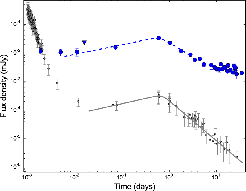
Figure 7.— Broken power law fit to the X-ray (grey, solid) and Swift/UVOT White-band light curves for GRB 100418A near the re-brightening around 0.6 d. The X-ray fit includes points between 0.02 and 50 d, while the White-band fit includes points between $6\times 10^{-3}$ and 3.1 d. A joint fit yields the best fit parameters $t_{\rm b}=0.58^{+0.37}_{-0.34}$ d, $\alpha_{1}=0.42^{+0.31}_{-0.13}$, and $\alpha_{2}=-1.10^{+0.15}_{-0.21}$, with a fixed value of $y=5.0$ (Section 6.1.1).

We extract XRT spectra at 0.06–0.08 d (mean photon arrival 0.07 d), and at 0.58–1.81 d (mean photon arrival 0.88 d). We extrapolate the second SED to 1.5 d and show the complete optical to X-ray SED at 0.07 d and 1.5 d in Figure 8. The spectral index between the UVOT $B$-band observation at 0.07 d and the X-rays is $\beta_{\rm opt-X}=-0.93\pm 0.09$, which is consistent with the X-ray spectral index of $\beta_{\rm X}=-1.08\pm 0.18$ over this period, suggesting that the optical and X-ray are located on the same part of the afterglow SED at 0.07 d. The spectral index between the NIR and X-rays at 1.5 d is $\beta_{\rm NIR-X}=-0.94\pm 0.04$, which is consistent with the spectral index in the NIR and optical alone, $\beta_{\rm NIR-opt}=-0.8\pm 0.1$, once again suggesting that the NIR/optical and X-rays are located on the same part of the afterglow SED at 1.5 d and that intrinsic extinction is negligible. This implies that either $\nu_{\rm m}<\nu_{\rm NIR}<\nu_{\rm X}<\nu_{\rm c}$ with $p\approx 3$ or $\nu_{\rm m},\nu_{\rm c}<\nu_{\rm NIR}<\nu_{\rm X}$ with $p\approx 2$ at both 0.07 d and 1.5 d. If $\nu_{\rm m}<\nu_{\rm NIR}<\nu_{\rm X}<\nu_{\rm c}$ at 1.5 d, the decay rate would be $\alpha\approx-1.5$ in the ISM model or $\alpha\approx-2.0$ in the wind model, whereas in the latter we would expect $\alpha\approx-1$ in both ISM and wind scenarios. The observed UV/NIR/X-ray common decay rate after the re-brightening of $\alpha\approx-1$ indicates that $\nu_{\rm m},\nu_{\rm c}<\nu_{\rm NIR}<\nu_{\rm X}$ at 1.5 d and $p\approx 2$.

The 8.46 GHz light curve drops as $t^{-2.5}$ between the ATCA observation at 2 d and the VLA observation at 3 d, while the SMA 345 GHz light curve is flat over this period (Figure 9). At $\approx$2 d, the radio spectral index is $\approx 0.7$ from 4.9 GHz to 8.46 GHz, and $\approx 0.3$ from 8.46 GHz to 345 GHz. The rapid decline in the light curve at a single waveband can not be explained in the standard synchrotron model by forward shock emission. We consider an alternative scenario, in which the radio to millimeter emission at 2 d is dominated by a reverse shock. In that case, the peak frequency of the reverse shock must pass through 8.46 GHz before 2 d with a peak flux density of at least $\approx 1.3$ mJy. Propagating the RS spectrum back in time assuming the peak frequency and peak flux evolve as $t^{-1.5}$ and $t^{-1}$ respectively (Kobayashi & Sari, 2000), we would expect a minimum $R$-band flux density of $\approx 2$ Jy at 120 s. This is more than five orders of magnitude brighter than Swift White-band observations at this time. Thus the rapid decline and re-brightening of the 8.46 GHz light curve between 2 and 20 d cannot be explained in the standard synchrotron framework. It is possible that these data suffer from strong ISS, and we therefore exclude these data from our analysis.

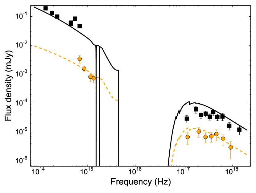
Figure 8.— Observed NIR to X-ray SED of the afterglow of GRB 100418A at 0.07 d (orange circles) and after the re-brightening (1.5 d; black squares), together with the best-fit ISM model (Section 6.1.2) including energy injection (Section 6.1.3) at 0.07 d (orange; dashed) and 1.5 d (black; solid). The data points and model at 0.07 d have been multiplied by a factor of 0.1 for clarity. The XRT SED at 1.5 d has been extrapolated from 0.88 d using the best-fit broken power law model to the XRT light curve (Figure 7; the correction factor is $\approx 0.5$). The optical data have been extrapolated using the best fit to the Swift/UVOT light curve (the corrections are small at $<5\%$). The cooling break (visible in the orange, dashed curve at $\approx 3\times 10^{14}$ Hz) is already below the optical bands at 0.07; the NIR to X-ray frequencies are therefore on the same part of the afterglow SED at 1.5 d.

6.1.2 Forward shock model at $t\gtrsim 0.4$ d

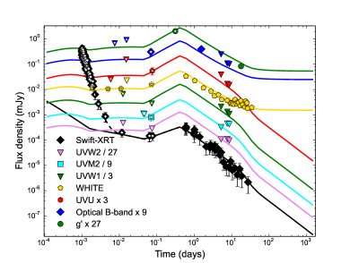
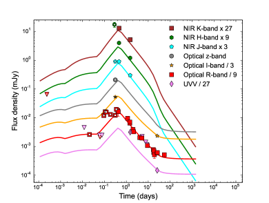
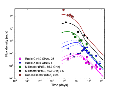
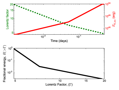
Figure 9.— X-ray, UV (top left), optical (top right), and radio (bottom left) light curves of GRB 100418A, with the full afterglow model (solid lines), including energy injection before 0.04 d. The X-ray data before 0.008 d is likely dominated by high-latitude prompt emission and we do not include these data in our analysis; the best fit power law to the X-ray data before 0.008 d added to the blastwave model is shown in the upper left panel (black, dashed). The dashed envelopes around the radio light curves indicate the expected effect of scintillation at the $1\sigma$ level. The data indicated by open symbols are not used to determine the parameters of the forward shock (the MCMC analysis). Bottom right: blastwave Lorentz factor (green, dashed; upper sub-panel) and isotropic equivalent kinetic energy (red, solid; upper sub-panel) as a function of time, together with the energy distribution across ejecta Lorentz factors (black, solid; lower sub-panel) as determined from fitting the X-ray/UV/optical re-brightening at 0.7 d.

The optical and X-ray light curves after 0.4 d are insensitive to the circumburst density profile since $\nu_{\rm m},\nu_{\rm c}<\nu_{\rm NIR}<\nu_{\rm X}$ after the re-brightening. The best-sampled radio light curve is the composite 8.46 GHz formed from VLA, VLBA, and ATCA observations. However, this light curve exhibits significant scatter about a smooth power law evolution, possibly due to either ISS or inter-calibration issues across the three telescopes. Thus we are unable to constrain the circumburst density profile from the afterglow data. For the remainder of this section we focus on the ISM model, discussing the possibility of a wind environment in Appendix C.

Since this event occurred at a relatively low redshift, $z=0.6235$ (Antonelli et al., 2010), the host galaxy is detected in the Sloane Digital Sky Survey (SDSS) as SDSS J170527.10+112742.5. We use the SDSS photometry ($u=24.55\pm 1.14$, $g=22.92\pm 0.17$, $r=22.45\pm 0.17$, $i=21.95\pm 0.17$, $z=22.54\pm 0.83$) as fixed a-priori measurements of the host galaxy flux in the $griz$ bands. We compute the host flux density at $B$- and $V$-band using $B=g+0.33(g-r)+0.2$ and $V=g-0.58(g-r)-0.01$ (Jester et al., 2005) and hold these values fixed for our MCMC analysis. Since there is no a-priori measurement of the host flux density in the UVOT/White-band and much of the UVOT data was taken in White-band, we keep the host flux density in the White-band as a free parameter, and integrate over the GRB spectral energy distribution using the White-band filter function.

Using our MCMC analysis as described in Section 4, we fit the data after 0.4 d, and our highest-likelihood model (Figure 9) has the parameters $p\approx 2.1$, $\epsilon_{\rm e}\approx 0.12$, $\epsilon_{B}\approx 1.1\times 10^{-2}$, $n_{0}\approx 1.4$ ${\rm cm}^{-3}$, $E_{\rm K,iso}\approx 3.4\times 10^{52}$ erg, $t_{\rm jet}\approx 17$ d, $A_{\rm V}\lesssim 0.1$ mag, and $F_{\nu,\rm host,White}\approx 1.6\,\mu$Jy, with a Compton $y$-parameter of $\approx 2.9$, indicating IC cooling is important. The blastwave Lorentz factor is $\Gamma=4.9(t/1\,{\rm d})^{-3/8}$ and the jet opening angle is $\theta_{\rm jet}\approx 20\arcdeg$. The beaming-corrected kinetic energy is $E_{\rm K}\approx 2.1\times 10^{51}\,{\rm erg}$, while the beaming corrected $\gamma$-ray energy is $E_{\gamma}\approx 6\times 10^{49}\,{\rm erg}$ (1–$10^{4}$ keV; rest frame), corresponding to an extremely low radiative efficiency of $\eta_{\rm rad}\equiv E_{\gamma}/(E_{\rm K}+E_{\gamma})\approx 3\%$. These results are summarized in Table 5. We present histograms of the marginalized posterior density for all parameters in Figure 10 and contour plots of correlations between the physical parameters in Figure 11.

In concordance with the basic analysis outlined above, we find that the break frequencies at 1 d for this model are located at $\nu_{\rm a}\approx 9.0$ GHz, $\nu_{\rm m}\approx 3.4\times 10^{11}$ Hz, and $\nu_{\rm c}\approx 2.3\times 10^{14}$ Hz, while the peak flux density is about 12 mJy at $\nu_{\rm m}$. The spectrum transitions from fast to slow cooling at about 230 s after the burst, and $\nu_{\rm m}$ drops below $\nu_{\rm a}$ at about 25 d. The high value of $\nu_{\rm a}$ is required to suppress the flux density at $8.46$ GHz and $5$ GHz (VLA), relative to the mm-band (PdBI and SMA). The ordering of the break frequencies relative to the observing bands, $\nu_{\rm m},\nu_{\rm c}<\nu_{\rm NIR}$ at 1 d, ensures that the optical and X-ray are on the same part of the synchrotron spectrum at this time. The jet break at $\approx 17$ d is largely driven by the millimeter and radio data. The blastwave becomes non-relativistic at $t_{\rm NR}\approx 40$ d, resulting in a subsequent slow decline ($F_{\nu}\sim t^{0.6+3\beta}\sim t^{-1}$, with $\beta=(1-p)/2\approx-0.5$; Frail et al. 2000) in the radio light curves after the peak.

Moin et al. (2013) use a VLBA limit on the size of the afterglow at 65 d to estimate the average ejecta Lorentz factor. However, we note that the apparent physical size of the afterglow is given by $R_{\perp}=\left[2^{12-3k}(4-k)^{5-k}/(5-k)^{5-k}\right]^{1/(8-2k)}\Gamma ct_{\rm z}\approx 2.3\Gamma ct_{\rm z}$, where $\gamma_{l}$ is the ejecta Lorentz factor of the ejecta at time, $t_{\rm z}=t_{\rm obs}/(1+z)$, and $k=0$ for the ISM model (Granot & Sari, 2002); therefore the VLBI measurement actually represents an upper limit to the ejecta Lorentz factor at the time of the measurement, such that $\Gamma(t_{\rm obs}=65\,\rm d)<5.8$. Since the blastwave becomes non-relativistic at around 40 days, our model does not violate the VLBA limit on the angular size of the afterglow.

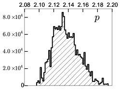
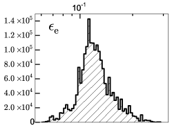
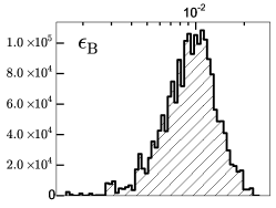
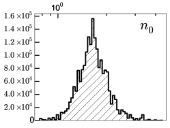
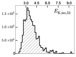
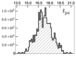
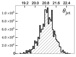
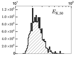
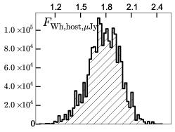
Figure 10.— Posterior probability density functions for the physical parameters for GRB 100418A in a constant density environment from MCMC simulations.

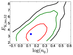
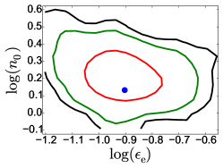
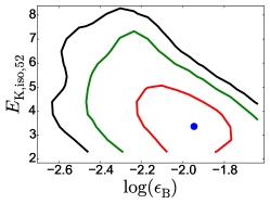
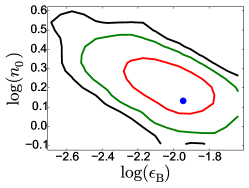
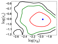
Figure 11.— 1$\sigma$ (red), 2$\sigma$ (green), and 3$\sigma$ (black) contours for correlations between the physical parameters, $E_{\rm K,iso}$, $n_{0}$, $\epsilon_{\rm e}$, and $\epsilon_{B}$ for GRB 100418A, in the ISM model from Monte Carlo simulations. We have restricted $\epsilon_{\rm e}<\nicefrac{{1}}{{3}}$ and $\epsilon_{\rm B}<\nicefrac{{1}}{{3}}$. See the on line version of this Figure for additional plots of correlations between these parameters and $p$, $t_{\rm jet}$, $\theta_{\rm jet}$, $E_{\rm K}$, and $F_{\nu,\rm host,White}$.

6.1.3 Energy injection model

Taking the forward shock model described in Section 6.1.2 as a starting point, we find that the X-ray and UV/optical data before the re-brightening can be explained by two successive periods of energy injection,

$$E_{\rm K,iso}(t)=\begin{cases}E_{\rm K,iso,f},&t>t_{\rm 0}=0.45\,{\rm d}\\ E_{\rm K,iso,f}\left(\frac{t}{t_{\rm 0}}\right)^{1.55},&t_{1}=0.05\,{\rm d}<t<t_{\rm 0}\\ E_{\rm K,iso,f}\left(\frac{t_{1}}{t_{\rm 0}}\right)^{1.55}\left(\frac{t}{t_{1}}\right)^{0.7},&t_{2}=1.7\times 10^{-3}\,{\rm d}<t<t_{1}\\ E_{\rm K,iso,f}\left(\frac{t_{1}}{t_{\rm 0}}\right)^{1.55}\left(\frac{t_{2}}{t_{1}}\right)^{0.7},&t<t_{2}\\ \end{cases}$$ (4)

In this model, the energy increases by a factor of $\approx 11$ from $E_{\rm K,iso,i}\approx 1.0\times 10^{50}$ erg at $1.7\times 10^{-3}$ d to $E_{\rm K,iso}\approx 1.1\times 10^{51}$ erg at 0.05 d followed by another increase by a factor of $\approx 30$ to $E_{\rm K,iso,f}\approx 3.4\times 10^{52}$ erg at 0.45 d. The overall increase in energy is a factor of $\approx 340$, corresponding to an injected energy fraction of $\approx 99.7\%$ over this period. In comparison, $E_{\gamma,\rm iso}=9.9^{+6.3}_{-3.4}\times 10^{50}$ (Marshall et al., 2011). The blastwave Lorentz factor decreases from $\Gamma\approx 38$ at the start of energy injection at $1.7\times 10^{-3}$ to $\Gamma\approx 11$ at $0.05$ d, and then to $\Gamma\approx 7$ at the end of energy injection at 0.45 d. The values of $m$ derived above correspond to an ejecta distribution with $E(>\Gamma)\propto\Gamma^{1-s}$ with $s\approx 9.6$ for $7\lesssim\Gamma\lesssim 11$ and $s\approx 3$ for $11\lesssim\Gamma\lesssim 38$.

6.2. GRB 100901A

6.2.1 GRB properties and basic considerations

GRB 100901A was detected and localized by the Swift BAT on 2010 September 01 at 13:34:10 UT (Immler et al., 2010). The burst duration is $T_{90}=(439\pm 33)$ s, with a fluence of $F_{\gamma}=(2.1\pm 0.3)\times 10^{-6}$ erg cm^-2 (15–150 keV observer frame; Immler et al., 2010). The afterglow was detected in the X-rays and optical bands by XRT (Page & Immler, 2010), UVOT (Pritchard & Immler, 2010), and by multiple ground-based observatories (e.g. De Cia et al., 2010; Kuroda et al., 2010c; Hentunen et al., 2010; Updike et al., 2010b; Sahu et al., 2010b; Kopac et al., 2010; Gorbovskoy et al., 2010; Pandey & Zheng, 2010), as well as in the radio by the WSRT and the VLA (van der Horst et al., 2010b; Chandra & Frail, 2010a). Spectroscopic observations with Magellan yielded a redshift of $z=1.408$ (Chornock et al., 2010). Using the BAT fluence, Gorbovskoy et al. (2012) determined the isotropic equivalent $\gamma$-ray energy of this burst to be $E_{\gamma,\rm iso}=6.3\times 10^{52}$ erg (1–$10^{4}$ keV; rest frame). However, the $\gamma$-ray spectrum does not exhibit a turnover within the BAT energy range, indicating that the peak of the $\gamma$-ray spectrum, $E_{\rm peak}$, is outside the BAT energy range. Margutti et al. (2013) obtain a correlation between $E_{\rm BAT,obs}$ (15–150 keV) and $E_{\rm\gamma,iso}$: $\frac{E_{\gamma,\rm iso}}{\rm erg}=10^{-3.7}\left[\frac{E_{\rm BAT}^{15--150}}{\rm erg}\right]^{1.08\pm 0.01}$ with a scatter of $\sigma=0.24$ (68%), which we use to perform a K-correction and obtain $E_{\gamma,\rm iso}=(8\pm 1)\times 10^{52}$ erg. Note that the error bars do not include the uncertainty in the correlation itself.

Table 7Swift/UVOT Observations of GRB 100901A

$t-t_{0}$	Filter	Frequency	Flux density†	Uncertainty	Detection?
(days)		(Hz)	($\mu$Jy)	($\mu$Jy)	($1=$ Yes)
0.00258	White	8.64e+14	27.4	5.65	1
0.00498	u	8.56e+14	146	11.4	1
0.00661	b	6.92e+14	230	75.6	0
0.00689	White	8.64e+14	58.6	18.9	1
0.00717	uvw2	1.48e+15	67.9	12.1	0
0.0454	v	5.55e+14	155	27	1
0.0478	uvm2	1.34e+15	18.3	4.42	1
0.0502	uvw1	1.16e+15	37.1	5.4	1
0.0597	uvw2	1.48e+15	7.4	2.36	0
0.0609	u	8.56e+14	83.4	6.21	1
0.062	v	5.55e+14	161	27.1	1
0.0632	b	6.92e+14	134	12.9	1
0.0644	uvm2	1.34e+15	20.7	4.63	1
0.0652	White	8.64e+14	62.2	9.12	1
0.0668	uvw1	1.16e+15	17.2	4.39	1
0.117	uvw2	1.48e+15	3.45	1.02	1
0.127	v	5.55e+14	97.7	12	1
0.137	uvm2	1.34e+15	10.1	2	1
0.183	uvw1	1.16e+15	42.7	3.03	1
0.194	u	8.56e+14	129	5.18	1
0.204	b	6.92e+14	192	10.2	1
0.25	uvm2	1.34e+15	21.3	2.22	1
0.261	uvw1	1.16e+15	58.3	3.6	1
0.271	u	8.56e+14	160	6.96	1
0.318	uvw2	1.48e+15	11.4	1.37	1
0.329	v	5.55e+14	291	15.5	1
0.338	uvm2	1.34e+15	26.6	2.92	1
0.384	uvw1	1.16e+15	40.4	8.67	1
0.534	uvw1	1.16e+15	36.8	2.88	1
0.541	u	8.56e+14	107	10.1	1
0.599	uvw2	1.48e+15	6.15	1.19	1
0.607	v	5.55e+14	178	28.3	1
0.647	b	6.92e+14	130	43.4	0
0.717	uvm2	1.34e+15	8.27	2.26	1
0.736	uvw1	1.16e+15	24.4	2.5	1
0.743	u	8.56e+14	63.4	13.4	1
0.786	uvw2	1.48e+15	3.82	1.01	1
0.796	v	5.55e+14	117	12.3	1
0.806	uvm2	1.34e+15	12.7	2.14	1
0.853	uvw1	1.16e+15	16.8	2.01	1
0.863	u	8.56e+14	54.4	3.36	1
0.873	b	6.92e+14	64.8	8.72	1
0.92	uvm2	1.34e+15	6.86	1.49	1
0.93	uvw1	1.16e+15	19.1	2.14	1
0.94	u	8.56e+14	41.4	4.63	1
0.983	uvw2	1.48e+15	7.57	2.11	0
1.06	v	5.55e+14	74.5	11.6	1
1.13	uvm2	1.34e+15	6.64	1.18	1
1.14	b	6.92e+14	51.5	8.67	1
1.15	uvw2	1.48e+15	2.53	0.828	0
1.16	uvw1	1.16e+15	12.2	1.35	1
1.17	u	8.56e+14	31	2.53	1
1.87	uvw2	1.48e+15	1.57	0.51	0
1.87	uvm2	1.34e+15	2.87	0.771	1
1.88	uvw1	1.16e+15	5.66	1.13	1
1.93	u	8.56e+14	15.5	1.74	1
1.94	b	6.92e+14	26.9	3.6	1
1.94	White	8.64e+14	10.7	1.69	1
1.94	v	5.55e+14	54.1	8.97	1
2.8	b	6.92e+14	17.4	5.28	1
2.8	White	8.64e+14	5.82	1.45	1
2.81	v	5.55e+14	35.6	11.7	0
2.86	u	8.56e+14	6.97	2.32	0
2.93	uvw2	1.48e+15	2.38	0.694	0
2.93	uvm2	1.34e+15	3.5	0.917	0
2.94	uvw1	1.16e+15	4.22	1.29	0
4.2	u	8.56e+14	8.36	2.64	0
4.2	uvw2	1.48e+15	3.99	0.955	0
4.27	b	6.92e+14	24.6	7.94	0
4.27	White	8.64e+14	5.56	1.89	0
4.28	v	5.55e+14	53.8	17.3	0
4.34	uvm2	1.34e+15	7.14	1.64	0
4.35	uvw1	1.16e+15	8.36	2.24	0
4.8	u	8.56e+14	8.03	2.61	0
4.8	uvw2	1.48e+15	4.13	1.1	0
4.8	b	6.92e+14	17.4	5.63	0
4.8	uvm2	1.34e+15	6.04	1.48	0
4.81	White	8.64e+14	3.98	1.36	0
4.81	uvw1	1.16e+15	7.16	1.97	0
4.81	v	5.55e+14	53.2	16.9	0
5.67	u	8.56e+14	33.1	9.34	0
5.8	uvw2	1.48e+15	10.1	2.13	0
7.24	uvw2	1.48e+15	1.39	0.394	0
7.25	uvm2	1.34e+15	1.83	0.542	0
7.25	uvw1	1.16e+15	2.41	0.758	0
9.46	v	5.55e+14	19.8	6.4	0
10.2	u	8.56e+14	3.96	1.28	0
10.2	b	6.92e+14	8.75	2.87	0
10.2	White	8.64e+14	2.05	0.678	0
11	u	8.56e+14	4.21	1.36	0
11	b	6.92e+14	9.31	3.05	0
11	White	8.64e+14	2.26	0.743	0
11	v	5.55e+14	23	7.48	0
11.7	u	8.56e+14	4.41	1.4	0
11.7	b	6.92e+14	9.97	3.23	0
11.7	White	8.64e+14	2.55	0.859	0
11.8	v	5.55e+14	30.4	9.91	0
12.6	u	8.56e+14	4.11	1.33	0
12.6	b	6.92e+14	8.96	2.94	0
12.6	White	8.64e+14	2.12	0.703	0
12.6	v	5.55e+14	23.1	7.59	0
13.5	b	6.92e+14	20.4	6.56	0
13.5	White	8.64e+14	5.14	1.68	0
13.5	v	5.55e+14	62	19.5	0
13.6	u	8.56e+14	8.12	2.58	0
14.6	u	8.56e+14	4.3	1.42	0
14.6	b	6.92e+14	9.41	3.08	0
14.7	White	8.64e+14	2.19	0.721	0
14.7	v	5.55e+14	23.5	7.62	0
15.7	u	8.56e+14	4.1	1.31	0
15.7	b	6.92e+14	8.93	2.95	0
15.7	White	8.64e+14	2.08	0.693	0
15.7	v	5.55e+14	22.7	7.38	0
16.7	u	8.56e+14	4.13	1.32	0
16.8	b	6.92e+14	9.21	2.99	0
16.8	White	8.64e+14	2.41	0.794	0
16.8	v	5.55e+14	24.8	8.08	0
17.7	u	8.56e+14	4.29	1.38	0
17.7	b	6.92e+14	9.39	3.09	0
17.7	White	8.64e+14	2.15	0.707	0
17.7	v	5.55e+14	21.8	7.11	0
18.6	u	8.56e+14	4.27	1.37	0
18.6	b	6.92e+14	9.32	3.04	0
18.6	White	8.64e+14	2.13	0.701	0
18.6	v	5.55e+14	21.3	6.85	0

Note. — ^†In cases of non-detections, we report the formal flux measurement at the position of the afterglow.

XRT began observing the GRB during the $\gamma$-ray emission interval. The X-ray spectra from 1 ks to the end of XRT observations are well fit by an absorbed single power law model with $N_{\rm H,Gal}=7.1\times 10^{20}\,{\rm cm}^{-2}$ (Kalberla et al., 2005), intrinsic hydrogen column $N_{\rm H,int}=(3.1\pm 0.7)\times 10^{21}\,{\rm cm}^{-2}$, and photon index, $\Gamma_{\rm X}=2.15\pm 0.06$, with no evidence for spectral evolution during this period. We convert the count rate light curve published by Margutti et al. (2013) to a flux density light curve at 1 keV using their time-resolved spectra. We also analyze all UVOT photometry for this burst and report our results in Table 7, and a compilation of all photometry listed in GCN circulars or published elsewhere for this event in Table 8.

Table 8Optical Observations of GRB 100901A

$t-t_{0}$	Observatory	Telescope /	Filter	Frequency	Flux density†	Uncertainty	Detection?	Reference
(days)		Instrument		(Hz)	($\mu$Jy)	($\mu$Jy)	($1=$ Yes)
0.00131	MASTER		CR	4.4e+14	82.1	436	0	Gorbovskoy et al. (2012)
0.00178	MASTER		CR	4.4e+14	156	170	0	Gorbovskoy et al. (2012)
0.00246	MASTER		CR	4.4e+14	131	143	0	Gorbovskoy et al. (2012)
0.00396	MASTER		CR	4.4e+14	119	107	0	Gorbovskoy et al. (2012)
0.00494	MASTER		CR	4.4e+14	304	78.6	1	Gorbovskoy et al. (2012)
0.00615	MASTER		CR	4.4e+14	125	73.4	0	Gorbovskoy et al. (2012)
0.00758	MASTER		CR	4.4e+14	88.4	80	0	Gorbovskoy et al. (2012)
0.0093	MASTER		CR	4.4e+14	109	80.6	0	Gorbovskoy et al. (2012)
0.0114	MASTER		CR	4.4e+14	204	65	1	Gorbovskoy et al. (2012)
0.012	Okayama	MITSuME	Ic	3.93e+14	460	93.1	1	Kuroda et al. (2010c)
0.012	Okayama	MITSuME	Rc	4.56e+14	336	32.4	1	Kuroda et al. (2010c)
0.012	Okayama	MITSuME	g’	6.29e+14	132	77.1	1	Kuroda et al. (2010c)
0.0136	MASTER		CR	4.4e+14	195	62.1	1	Gorbovskoy et al. (2012)
0.0159	MASTER		v	5.55e+14	292	55.8	1	Gorbovskoy et al. (2012)
0.0182	MASTER		CR	4.4e+14	232	74	1	Gorbovskoy et al. (2012)
0.0227	MASTER		v	5.55e+14	292	55.8	1	Gorbovskoy et al. (2012)
0.0251	MASTER		v	5.55e+14	351	59.4	1	Gorbovskoy et al. (2012)
0.0275	MASTER		CR	4.4e+14	228	22	1	Gorbovskoy et al. (2012)
0.0299	MASTER		CR	4.4e+14	224	12.7	1	Gorbovskoy et al. (2012)
0.0323	MASTER		CR	4.4e+14	202	11.5	1	Gorbovskoy et al. (2012)
0.0334	Okayama	MITSuME	Ic	3.93e+14	265	25.6	1	Kuroda et al. (2010c)
0.0334	Okayama	MITSuME	Rc	4.56e+14	212	20.5	1	Kuroda et al. (2010c)
0.0334	Okayama	MITSuME	g’	6.29e+14	209	20.2	1	Kuroda et al. (2010c)
0.0382	MASTER		CR	4.4e+14	186	12.4	1	Gorbovskoy et al. (2012)
0.0406	MASTER		CR	4.4e+14	195	13	1	Gorbovskoy et al. (2012)
0.043	MASTER		CR	4.4e+14	192	12.8	1	Gorbovskoy et al. (2012)
0.0454	MASTER		CR	4.4e+14	214	12.2	1	Gorbovskoy et al. (2012)
0.0478	MASTER		CR	4.4e+14	185	12.3	1	Gorbovskoy et al. (2012)
0.0502	MASTER		CR	4.4e+14	212	14.1	1	Gorbovskoy et al. (2012)
0.0526	MASTER		CR	4.4e+14	155	13.4	1	Gorbovskoy et al. (2012)
0.0548	Okayama	MITSuME	Ic	3.93e+14	220	21.3	1	Kuroda et al. (2010c)
0.0548	Okayama	MITSuME	Rc	4.56e+14	122	11.8	1	Kuroda et al. (2010c)
0.0548	Okayama	MITSuME	g’	6.29e+14	120	11.6	1	Kuroda et al. (2010c)
0.055	MASTER		CR	4.4e+14	117	13.6	1	Gorbovskoy et al. (2012)
0.0574	MASTER		CR	4.4e+14	109	15	1	Gorbovskoy et al. (2012)
0.0599	MASTER		CR	4.4e+14	183	14	1	Gorbovskoy et al. (2012)
0.0623	MASTER		CR	4.4e+14	185	14.1	1	Gorbovskoy et al. (2012)
0.0647	MASTER		CR	4.4e+14	186	14.3	1	Gorbovskoy et al. (2012)
0.067	MASTER		CR	4.4e+14	193	14.8	1	Gorbovskoy et al. (2012)
0.0695	MASTER		CR	4.4e+14	164	14.2	1	Gorbovskoy et al. (2012)
0.0721	MASTER		CR	4.4e+14	206	15.8	1	Gorbovskoy et al. (2012)
0.0745	MASTER		CR	4.4e+14	167	16.1	1	Gorbovskoy et al. (2012)
0.0759	Okayama	MITSuME	Ic	3.93e+14	152	30.8	1	Kuroda et al. (2010c)
0.0759	Okayama	MITSuME	Rc	4.56e+14	134	12.9	1	Kuroda et al. (2010c)
0.0759	Okayama	MITSuME	g’	6.29e+14	120	11.6	1	Kuroda et al. (2010c)
0.0804	MASTER		CR	4.4e+14	131	14	1	Gorbovskoy et al. (2012)
0.0828	MASTER		CR	4.4e+14	110	15.2	1	Gorbovskoy et al. (2012)
0.0852	MASTER		CR	4.4e+14	101	16	1	Gorbovskoy et al. (2012)
0.0877	MASTER		CR	4.4e+14	61.2	18.7	1	Gorbovskoy et al. (2012)
0.0901	MASTER		CR	4.4e+14	106	16.9	1	Gorbovskoy et al. (2012)
0.0926	MASTER		CR	4.4e+14	141	16.5	1	Gorbovskoy et al. (2012)
0.095	MASTER		CR	4.4e+14	156	18.3	1	Gorbovskoy et al. (2012)
0.0969	Okayama	MITSuME	Ic	3.93e+14	152	30.8	1	Kuroda et al. (2010c)
0.0969	Okayama	MITSuME	Rc	4.56e+14	122	11.8	1	Kuroda et al. (2010c)
0.0969	Okayama	MITSuME	g’	6.29e+14	100	9.65	1	Kuroda et al. (2010c)
0.118	Okayama	MITSuME	Ic	3.93e+14	167	33.8	1	Kuroda et al. (2010c)
0.118	Okayama	MITSuME	Rc	4.56e+14	101	20.5	1	Kuroda et al. (2010c)
0.118	Okayama	MITSuME	g’	6.29e+14	83.2	16.8	1	Kuroda et al. (2010c)
0.131	MASTER		CR	4.4e+14	22	25.7	0	Gorbovskoy et al. (2012)
0.134	MASTER		CR	4.4e+14	74.9	17.7	1	Gorbovskoy et al. (2012)
0.136	MASTER		CR	4.4e+14	58.9	18.8	1	Gorbovskoy et al. (2012)
0.139	MASTER		CR	4.4e+14	54.3	35	0	Gorbovskoy et al. (2012)
0.139	Okayama	MITSuME	Ic	3.93e+14	183	17.7	1	Kuroda et al. (2010c)
0.139	Okayama	MITSuME	Rc	4.56e+14	134	12.9	1	Kuroda et al. (2010c)
0.139	Okayama	MITSuME	g’	6.29e+14	110	10.6	1	Kuroda et al. (2010c)
0.141	MASTER		CR	4.4e+14	108	31.8	1	Gorbovskoy et al. (2012)
0.144	MASTER		CR	4.4e+14	152	30.8	1	Gorbovskoy et al. (2012)
0.146	MASTER		CR	4.4e+14	106	32.5	1	Gorbovskoy et al. (2012)
0.149	MASTER		CR	4.4e+14	185	29.3	1	Gorbovskoy et al. (2012)
0.151	MASTER		CR	4.4e+14	135	22.9	1	Gorbovskoy et al. (2012)
0.154	MASTER		CR	4.4e+14	193	18.7	1	Gorbovskoy et al. (2012)
0.16	Okayama	MITSuME	Ic	3.93e+14	319	30.7	1	Kuroda et al. (2010c)
0.16	Okayama	MITSuME	Rc	4.56e+14	193	18.7	1	Kuroda et al. (2010c)
0.16	Okayama	MITSuME	g’	6.29e+14	120	11.6	1	Kuroda et al. (2010c)
0.172	Hanle	HCT	R	4.56e+14	267	12.6	1	Sahu et al. (2010b)
0.172	MASTER		R	4.56e+14	180	92.3	0	Gorbovskoy et al. (2012)
0.178	Hanle	HCT	I	3.93e+14	356	16.8	1	Sahu et al. (2010b)
0.181	Okayama	MITSuME	Ic	3.93e+14	349	33.7	1	Kuroda et al. (2010c)
0.181	Okayama	MITSuME	Rc	4.56e+14	280	27	1	Kuroda et al. (2010c)
0.181	Okayama	MITSuME	g’	6.29e+14	191	18.4	1	Kuroda et al. (2010c)
0.182	Terksol	Z-600	R	4.56e+14	282	7.9	1	Andreev et al. (2010a)
0.183	MASTER		CR	4.4e+14	202	36.5	1	Gorbovskoy et al. (2012)
0.183	MASTER		R	4.56e+14	230	39	1	Gorbovskoy et al. (2012)
0.186	MASTER		CR	4.4e+14	220	14.7	1	Gorbovskoy et al. (2012)
0.186	MASTER		R	4.56e+14	290	30.9	1	Gorbovskoy et al. (2012)
0.188	MASTER		CR	4.4e+14	239	13.6	1	Gorbovskoy et al. (2012)
0.188	MASTER		R	4.56e+14	277	26.7	1	Gorbovskoy et al. (2012)
0.19	MASTER		R	4.56e+14	321	24.5	1	Gorbovskoy et al. (2012)
0.193	MASTER		R	4.56e+14	239	23.1	1	Gorbovskoy et al. (2012)
0.195	MASTER		R	4.56e+14	358	23.9	1	Gorbovskoy et al. (2012)
0.198	MASTER		R	4.56e+14	290	25.1	1	Gorbovskoy et al. (2012)
0.2	MASTER		R	4.56e+14	321	21.4	1	Gorbovskoy et al. (2012)
0.202	Okayama	MITSuME	Ic	3.93e+14	383	37	1	Kuroda et al. (2010c)
0.202	Okayama	MITSuME	Rc	4.56e+14	255	24.6	1	Kuroda et al. (2010c)
0.202	Okayama	MITSuME	g’	6.29e+14	229	22.1	1	Kuroda et al. (2010c)
0.202	MASTER		R	4.56e+14	339	22.6	1	Gorbovskoy et al. (2012)
0.205	MASTER		R	4.56e+14	269	20.6	1	Gorbovskoy et al. (2012)
0.207	MASTER		R	4.56e+14	287	19.1	1	Gorbovskoy et al. (2012)
0.21	MASTER		R	4.56e+14	324	21.6	1	Gorbovskoy et al. (2012)
0.212	MASTER		R	4.56e+14	304	20.2	1	Gorbovskoy et al. (2012)
0.214	MASTER		R	4.56e+14	318	18.1	1	Gorbovskoy et al. (2012)
0.217	MASTER		R	4.56e+14	330	18.7	1	Gorbovskoy et al. (2012)
0.219	MASTER		R	4.56e+14	301	17.1	1	Gorbovskoy et al. (2012)
0.222	MASTER		R	4.56e+14	309	17.6	1	Gorbovskoy et al. (2012)
0.223	MASTER		R	4.56e+14	304	38.6	1	Gorbovskoy et al. (2012)
0.224	Okayama	MITSuME	Ic	3.93e+14	383	37	1	Kuroda et al. (2010c)
0.224	Okayama	MITSuME	Rc	4.56e+14	280	27	1	Kuroda et al. (2010c)
0.224	Okayama	MITSuME	g’	6.29e+14	191	18.4	1	Kuroda et al. (2010c)
0.224	MASTER		R	4.56e+14	321	18.2	1	Gorbovskoy et al. (2012)
0.226	MASTER		I	3.93e+14	383	33.1	1	Gorbovskoy et al. (2012)
0.226	MASTER		R	4.56e+14	355	20.2	1	Gorbovskoy et al. (2012)
0.227	MASTER		R	4.56e+14	324	18.4	1	Gorbovskoy et al. (2012)
0.228	MASTER		I	3.93e+14	397	34.3	1	Gorbovskoy et al. (2012)
0.228	MASTER		R	4.56e+14	293	19.5	1	Gorbovskoy et al. (2012)
0.229	MASTER		R	4.56e+14	400	18.9	1	Gorbovskoy et al. (2012)
0.23	MASTER		I	3.93e+14	359	34.6	1	Gorbovskoy et al. (2012)
0.23	MASTER		R	4.56e+14	333	18.9	1	Gorbovskoy et al. (2012)
0.231	MASTER		R	4.56e+14	327	18.6	1	Gorbovskoy et al. (2012)
0.233	MASTER		I	3.93e+14	432	33	1	Gorbovskoy et al. (2012)
0.233	MASTER		R	4.56e+14	352	20	1	Gorbovskoy et al. (2012)
0.233	MASTER		v	5.55e+14	410	43.7	1	Gorbovskoy et al. (2012)
0.234	MASTER		R	4.56e+14	321	18.2	1	Gorbovskoy et al. (2012)
0.235	MASTER		I	3.93e+14	369	31.9	1	Gorbovskoy et al. (2012)
0.235	MASTER		R	4.56e+14	324	18.4	1	Gorbovskoy et al. (2012)
0.235	MASTER		v	5.55e+14	371	43.3	1	Gorbovskoy et al. (2012)
0.236	MASTER		R	4.56e+14	365	17.2	1	Gorbovskoy et al. (2012)
0.237	MASTER		I	3.93e+14	369	31.9	1	Gorbovskoy et al. (2012)
0.237	MASTER		R	4.56e+14	372	17.5	1	Gorbovskoy et al. (2012)
0.239	MASTER		R	4.56e+14	382	18	1	Gorbovskoy et al. (2012)
0.24	MASTER		I	3.93e+14	366	31.6	1	Gorbovskoy et al. (2012)
0.24	MASTER		R	4.56e+14	330	18.7	1	Gorbovskoy et al. (2012)
0.241	MASTER		R	4.56e+14	330	18.7	1	Gorbovskoy et al. (2012)
0.242	MASTER		I	3.93e+14	448	29.8	1	Gorbovskoy et al. (2012)
0.242	MASTER		R	4.56e+14	330	18.7	1	Gorbovskoy et al. (2012)
0.243	MASTER		R	4.56e+14	312	20.8	1	Gorbovskoy et al. (2012)
0.245	MASTER		I	3.93e+14	456	30.4	1	Gorbovskoy et al. (2012)
0.245	MASTER		R	4.56e+14	352	20	1	Gorbovskoy et al. (2012)
0.246	MASTER		R	4.56e+14	342	19.4	1	Gorbovskoy et al. (2012)
0.247	MASTER		I	3.93e+14	412	27.5	1	Gorbovskoy et al. (2012)
0.247	MASTER		R	4.56e+14	355	16.7	1	Gorbovskoy et al. (2012)
0.248	MASTER		R	4.56e+14	336	19.1	1	Gorbovskoy et al. (2012)
0.249	MASTER		I	3.93e+14	460	30.7	1	Gorbovskoy et al. (2012)
0.249	MASTER		R	4.56e+14	342	16.1	1	Gorbovskoy et al. (2012)
0.251	MASTER		R	4.56e+14	318	21.2	1	Gorbovskoy et al. (2012)
0.252	MASTER		I	3.93e+14	412	27.5	1	Gorbovskoy et al. (2012)
0.252	MASTER		R	4.56e+14	352	16.6	1	Gorbovskoy et al. (2012)
0.253	MASTER		R	4.56e+14	309	20.6	1	Gorbovskoy et al. (2012)
0.254	MASTER		I	3.93e+14	529	30	1	Gorbovskoy et al. (2012)
0.254	MASTER		R	4.56e+14	330	15.5	1	Gorbovskoy et al. (2012)
0.256	MASTER		R	4.56e+14	358	20.4	1	Gorbovskoy et al. (2012)
0.257	MASTER		I	3.93e+14	482	27.4	1	Gorbovskoy et al. (2012)
0.257	MASTER		R	4.56e+14	372	17.5	1	Gorbovskoy et al. (2012)
0.257	Hanle	HCT	R	4.56e+14	355	16.7	1	Sahu et al. (2010b)
0.258	MASTER		R	4.56e+14	372	21.1	1	Gorbovskoy et al. (2012)
0.259	MASTER		I	3.93e+14	444	25.2	1	Gorbovskoy et al. (2012)
0.259	MASTER		R	4.56e+14	375	14.1	1	Gorbovskoy et al. (2012)
0.261	MASTER		R	4.56e+14	431	20.3	1	Gorbovskoy et al. (2012)
0.261	MASTER		I	3.93e+14	505	23.8	1	Gorbovskoy et al. (2012)
0.262	Hanle	HCT	I	3.93e+14	465	17.4	1	Sahu et al. (2010b)
0.264	MASTER		I	3.93e+14	519	24.5	1	Gorbovskoy et al. (2012)
0.266	MASTER		I	3.93e+14	440	25	1	Gorbovskoy et al. (2012)
0.269	MASTER		I	3.93e+14	496	28.2	1	Gorbovskoy et al. (2012)
0.271	MASTER		I	3.93e+14	491	27.9	1	Gorbovskoy et al. (2012)
0.273	MASTER		I	3.93e+14	482	27.4	1	Gorbovskoy et al. (2012)
0.274	Terksol	Z-600	R	4.56e+14	349	6.48	1	Andreev et al. (2010b)
0.276	MASTER		I	3.93e+14	452	25.7	1	Gorbovskoy et al. (2012)
0.278	MASTER		I	3.93e+14	469	26.6	1	Gorbovskoy et al. (2012)
0.281	MASTER		I	3.93e+14	405	27	1	Gorbovskoy et al. (2012)
0.283	MASTER		I	3.93e+14	448	25.4	1	Gorbovskoy et al. (2012)
0.286	MASTER		I	3.93e+14	534	30.3	1	Gorbovskoy et al. (2012)
0.288	MASTER		I	3.93e+14	448	29.8	1	Gorbovskoy et al. (2012)
0.29	MASTER		I	3.93e+14	482	27.4	1	Gorbovskoy et al. (2012)
0.293	MASTER		I	3.93e+14	514	29.2	1	Gorbovskoy et al. (2012)
0.295	MASTER		I	3.93e+14	376	28.8	1	Gorbovskoy et al. (2012)
0.296	MASTER		v	5.55e+14	303	54.6	1	Gorbovskoy et al. (2012)
0.297	MASTER		I	3.93e+14	432	28.8	1	Gorbovskoy et al. (2012)
0.299	MASTER		v	5.55e+14	341	50.5	1	Gorbovskoy et al. (2012)
0.3	MASTER		I	3.93e+14	465	26.4	1	Gorbovskoy et al. (2012)
0.302	Golovec	Vega	R	4.56e+14	306	29.6	1	Kopac et al. (2010)
0.302	MASTER		I	3.93e+14	416	31.8	1	Gorbovskoy et al. (2012)
0.305	MASTER		I	3.93e+14	452	34.6	1	Gorbovskoy et al. (2012)
0.307	MASTER		I	3.93e+14	369	35.6	1	Gorbovskoy et al. (2012)
0.317	THO	C-14	CR	4.4e+14	333	32.1	1	Hentunen et al. (2010)
0.32	THO	C-14	CR	4.4e+14	304	61.4	1	Hentunen et al. (2010)
0.353	Terksol	Meade-35	v	5.55e+14	338	15.9	1	Andreev et al. (2010e)
0.355	Hanle	HCT	R	4.56e+14	339	12.7	1	Sahu et al. (2010b)
0.37	Terksol	Zeiss-2000	b	6.92e+14	232	4.31	1	Andreev et al. (2010e)
0.416	Gnosca	0.4m	CR	4.4e+14	304	96.6	1	Sposetti & Immler (2010)
0.427	Gnosca	0.4m	CR	4.4e+14	285	90.6	1	Sposetti & Immler (2010)
0.439	Gnosca	0.4m	CR	4.4e+14	287	91.4	1	Sposetti & Immler (2010)
0.442	THO	C-14	CR	4.4e+14	277	26.7	1	Hentunen et al. (2010)
0.449	Terksol	Zeiss-2000	b	6.92e+14	169	3.15	1	Andreev et al. (2010e)
0.45	Gnosca	0.4m	CR	4.4e+14	277	88.1	1	Sposetti & Immler (2010)
0.458	Terksol	Zeiss-2000	v	5.55e+14	266	4.94	1	Andreev et al. (2010e)
0.461	Gnosca	0.4m	CR	4.4e+14	246	78.2	1	Sposetti & Immler (2010)
0.464	Terksol	Zeiss-2000	r’	4.56e+14	263	4.89	1	Andreev et al. (2010e)
0.464	THO	C-14	Rc	4.56e+14	253	24.4	1	Hentunen et al. (2010)
0.468	THO	C-14	b	6.92e+14	234	47.3	1	Hentunen et al. (2010)
0.471	Terksol	Zeiss-2000	g’	6.29e+14	163	3.03	1	Andreev et al. (2010e)
0.472	Gnosca	0.4m	CR	4.4e+14	243	77.5	1	Sposetti & Immler (2010)
0.483	Gnosca	0.4m	CR	4.4e+14	267	85	1	Sposetti & Immler (2010)
0.494	Gnosca	0.4m	CR	4.4e+14	253	80.4	1	Sposetti & Immler (2010)
0.505	Gnosca	0.4m	CR	4.4e+14	246	78.2	1	Sposetti & Immler (2010)
0.505	NOT	ALFOSC	R	4.56e+14	277	88.1	1	De Cia et al. (2010)
0.516	Gnosca	0.4m	CR	4.4e+14	232	74	1	Sposetti & Immler (2010)
0.527	Gnosca	0.4m	CR	4.4e+14	210	66.9	1	Sposetti & Immler (2010)
0.539	Gnosca	0.4m	CR	4.4e+14	218	69.4	1	Sposetti & Immler (2010)
0.551	Gnosca	0.4m	CR	4.4e+14	216	68.7	1	Sposetti & Immler (2010)
0.562	Gnosca	0.4m	CR	4.4e+14	218	69.4	1	Sposetti & Immler (2010)
0.574	Gnosca	0.4m	CR	4.4e+14	206	65.6	1	Sposetti & Immler (2010)
0.585	Gnosca	0.4m	CR	4.4e+14	195	62.1	1	Sposetti & Immler (2010)
0.782	KPNO	SARA-N	b	6.92e+14	135	13	1	Updike et al. (2010b)
0.785	KPNO	SARA-N	v	5.55e+14	234	22.6	1	Updike et al. (2010b)
0.787	KPNO	SARA-N	R	4.56e+14	145	14	1	Updike et al. (2010b)
0.79	KPNO	SARA-N	I	3.93e+14	148	14.3	1	Updike et al. (2010b)
0.856	ISON-NM	0.45m	CR	4.4e+14	147	4.11	1	Elenin et al. (2010a)
1.05	Ishigakijima	Murikabushi	Ic	3.93e+14	121	5.71	1	Kuroda et al. (2010b)
1.05	Ishigakijima	Murikabushi	Rc	4.56e+14	87.6	3.29	1	Kuroda et al. (2010b)
1.05	Ishigakijima	Murikabushi	g’	6.29e+14	58.1	2.18	1	Kuroda et al. (2010b)
1.07	Hiroshima	Kanata	Rc	4.56e+14	82.1	7.92	1	Yoshida et al. (2010)
1.08	Hiroshima	Kanata	Rc	4.56e+14	83.6	5.57	1	Yoshida et al. (2010)
1.09	Ishigakijima	Murikabushi	Ic	3.93e+14	105	5.94	1	Kuroda et al. (2010b)
1.09	Ishigakijima	Murikabushi	Rc	4.56e+14	82.1	3.08	1	Kuroda et al. (2010b)
1.09	Ishigakijima	Murikabushi	g’	6.29e+14	53	1.99	1	Kuroda et al. (2010b)
1.1	Hiroshima	Kanata	Rc	4.56e+14	88.4	3.32	1	Yoshida et al. (2010)
1.14	Ishigakijima	Murikabushi	Ic	3.93e+14	96.2	6.41	1	Kuroda et al. (2010b)
1.14	Ishigakijima	Murikabushi	Rc	4.56e+14	69.6	2.61	1	Kuroda et al. (2010b)
1.14	Ishigakijima	Murikabushi	g’	6.29e+14	50.6	2.38	1	Kuroda et al. (2010b)
1.18	Okayama	MITSuME	Ic	3.93e+14	96.2	9.28	1	Kuroda et al. (2010d)
1.18	Okayama	MITSuME	Rc	4.56e+14	77	7.43	1	Kuroda et al. (2010d)
1.18	Okayama	MITSuME	g’	6.29e+14	63.1	6.09	1	Kuroda et al. (2010d)
1.22	Hanle	HCT	R	4.56e+14	75.6	7.29	1	Sahu et al. (2010a)
1.24	Hanle	HCT	I	3.93e+14	92.7	13.7	1	Sahu et al. (2010a)
1.3	MASTER		I	3.93e+14	90.2	3.39	1	Gorbovskoy et al. (2012)
1.38	Tautenburg	TLS1.34m	Rc	4.56e+14	66.4	1.86	1	Kann et al. (2010a)
1.39	Tautenburg	TLS1.34m	Rc	4.56e+14	61.7	2.32	1	Kann et al. (2010a)
1.42	Tautenburg	TLS1.34m	Rc	4.56e+14	59.5	1.67	1	Kann et al. (2010a)
1.43	Tautenburg	TLS1.34m	Rc	4.56e+14	55.3	1.55	1	Kann et al. (2010a)
1.43	Tautenburg	TLS1.34m	Rc	4.56e+14	61.2	2.29	1	Kann et al. (2010a)
1.44	Tautenburg	TLS1.34m	Rc	4.56e+14	65.2	2.45	1	Kann et al. (2010a)
1.46	Terksol	Z-600	R	4.56e+14	62.9	2.96	1	Andreev et al. (2010c)
1.7	Lightbuckets	0.61m	R	4.56e+14	46.8	14.9	0	Ukwatta et al. (2010)
2.13	Ishigakijima	Murikabushi	Ic	3.93e+14	23.3	3.95	1	Kuroda et al. (2010b)
2.13	Ishigakijima	Murikabushi	Rc	4.56e+14	31.8	1.81	1	Kuroda et al. (2010b)
2.13	Ishigakijima	Murikabushi	g’	6.29e+14	18.9	1.44	1	Kuroda et al. (2010b)
2.3	CrAO	AZT-11	R	4.56e+14	28.7	2.2	1	Rumyantsev et al. (2010)
2.41	Terksol	Z-600	R	4.56e+14	27.2	3.18	1	Andreev et al. (2010d)
2.43	Terksol	Z-600	R	4.56e+14	23.7	3.76	1	Andreev et al. (2010d)
2.83	ISON-NM	0.45m	CR	4.4e+14	24.1	6.25	1	Elenin et al. (2010b)
2.88	UKIRT		K	1.37e+14	47.6	9.64	1	Im et al. (2010)
3.31	Tautenburg	TLS1.34m	Rc	4.56e+14	18.8	1.25	1	Kann et al. (2010a)
3.55	Tautenburg	TLS1.34m	Rc	4.56e+14	16.1	0.604	1	Kann et al. (2010a)
3.82	ISON-NM	0.45m	CR	4.4e+14	13.9	2.81	1	Elenin et al. (2010b)
4.26	Ishigakijima	Murikabushi	Ic	3.93e+14	29.1	9.25	0	Kuroda et al. (2010a)
4.26	Ishigakijima	Murikabushi	Rc	4.56e+14	9.26	2.95	0	Kuroda et al. (2010a)
4.26	Ishigakijima	Murikabushi	g’	6.29e+14	8.32	2.65	0	Kuroda et al. (2010a)
4.4	Tautenburg	TLS1.34m	Rc	4.56e+14	9.26	0.436	1	Kann et al. (2010a)
4.4	CrAO	AZT-11	R	4.56e+14	11.1	2.25	1	Rumyantsev et al. (2010)
4.42	Tautenburg	TLS1.34m	Rc	4.56e+14	9.17	2.48	1	Kann et al. (2010a)
4.43	Tautenburg	TLS1.34m	Rc	4.56e+14	8.68	1.1	1	Kann et al. (2010a)
4.56	Tautenburg	TLS1.34m	Rc	4.56e+14	9.51	0.918	1	Kann et al. (2010a)
4.87	ISON-NM	0.45m	CR	4.4e+14	8.06	1.81	1	Elenin et al. (2010b)
5.55	Tautenburg	TLS1.34m	Rc	4.56e+14	5.28	0.563	1	Kann et al. (2010b)
6.3	Maidanak	AZT-22	R	4.56e+14	4.64	0.401	1	Volnova et al. (2010)

Note. — ^†In cases of non-detections, we report the formal flux measurement at the position of the afterglow.

The X-ray data before the first orbital gap at around $10^{-2}$ d exhibits rapid flaring, ending in a steep decay. The earliest UVOT observations during this period detect a counterpart at multiple wavelengths. Owing to the contemporaneous $\gamma$-ray emission, indicating on-going central engine activity during this period, we do not consider data before the first orbital gap for our afterglow analysis. The X-ray re-brightening and subsequent fading between 0.08 d and 20 d can be well fit with a broken power law model (Equation 5), with $t_{\rm b}=0.40\pm 0.02$ d, $F_{\nu,\rm X}(t_{\rm b})=2.0\pm 0.1\,\mu$Jy, $\alpha_{1}=0.77\pm 0.15$, $\alpha_{2}=-1.55\pm 0.06$, and $y=2.3\pm 1.1$ (Figure 12).

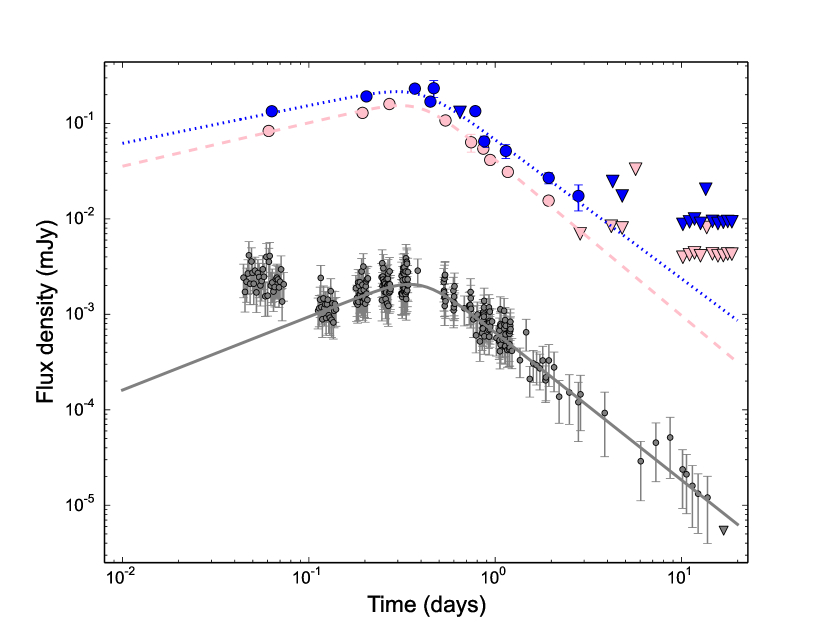
Figure 12.— Broken power law fit to the X-ray (grey, solid), Swift/UVOT $U$-band (pink, dashed), and Swift/UVOT $B$-band (blue, dotted) light curves for GRB 100901A near the re-brightening around 0.6 d. The X-ray fit includes points between 0.08 and 20 d, while the $U$- and $B$-band fits include points between $0.02$ d and 20 d. A joint fit yields the best fit parameters $t_{\rm b}=0.36\pm 0.02$, $\alpha_{1}=0.57\pm 0.09$, and $\alpha_{2}=-1.47\pm 0.07$ (Section 6.2.1).

A broken power law fit to the UVOT $U$-band data between $0.02$ d and 20 d yields $t_{\rm b}=0.40\pm 0.03$ d, $F_{\nu,\rm U}(t_{\rm b})=144\pm 7\,\mu$Jy, $\alpha_{1}=0.45\pm 0.06$, and $\alpha_{2}=-1.63\pm 0.12$, with $y=2.5$, similar to the results from fitting the X-ray re-brightening. Over the same time range, a broken power law fit to the UVOT $B$-band data yields $t_{\rm b}=0.39\pm 0.08$ d, $F_{\nu,\rm B}(t_{\rm b})=201\pm 24\,\mu$Jy, $\alpha_{1}=0.40\pm 0.06$, and $\alpha_{2}=-1.46\pm 0.21$, similar to the X-ray and $U$-band fits. Finally, we fit the X-ray, UVOT $U$-band and UVOT $B$-band data jointly, where we constrain the model light curves at the two frequencies to have the same rise and decay rate and time of peak, and use independent normalizations in the three bands. Using a Markov Chain Monte Carlo simulation using emcee (Foreman-Mackey et al., 2013), we find $t_{\rm b}=0.36\pm 0.02$, $\alpha_{1}=0.57\pm 0.09$, and $\alpha_{2}=-1.47\pm 0.07$, with a fixed value of $y=2.5$.

The spectral index between the UKIRT $K$-band observation at 2.88 d (Im et al., 2010) and the X-rays is $\beta_{\rm NIR,X}=-0.78\pm 0.08$. The spectral index between the NIR $K$-band and the Swift/$U$-band is slightly steeper, $\beta_{\rm NIR,UV}=-1.0\pm 0.2$, indicating that some extinction may be present. The spectral slope in the X-rays following the re-brightening is $\beta_{\rm X}=-1.15\pm 0.06$, leading to $\beta_{\rm NIR,X}-\beta_{\rm X}=0.4\pm 0.1$ suggesting that $\nu_{\rm opt}<\nu_{\rm c}<\nu_{\rm X}$ at 2.88 d.

If the X-rays indeed lie above $\nu_{\rm c}$, we would have $p=-2\beta_{\rm X}=2.3\pm 0.12$. The expected light curve decay rate is $\alpha=(2-3p)/4=-1.2\pm 0.1$ above $\nu_{\rm c}$ and $\alpha=3(1-p)/4=-1.0\pm 0.1$ (ISM) or $\alpha=-1.5\pm 0.1$ (wind) below $\nu_{\rm c}$. The $U$-band light curve after the re-brightening can be fit either with a single power law with $\alpha=-1.5$ or with a break from $\alpha\approx-0.9$ to $\alpha\approx-1.8$ at $\approx 1$ d and $\alpha=-1.0\pm 0.1$ between 0.2 d and 1.0 d. The former is consistent with a wind-like environment, while the latter suggests an ISM model and a jet break at $\approx 1$ d. We return to this point later.

Extrapolating the Lightbuckets $R$-band data at 1.7 d to the time of the SMA 345 GHz upper limit at 1.8 days using the fit to the optical $U$-band light curve described above, we find a spectral index of $\beta_{\rm mm-R}\gtrsim-0.6$ from the millimeter to the optical at this time. Combined with the steeper spectrum of $\beta_{\rm NIR,X}=-0.78\pm 0.08$ between the optical and X-rays, this suggests that the spectrum turns over above the millimeter band, indicating that $\nu_{\rm m}\gtrsim 345$ GHz at 1.8 d.

The spectral index between the VLA 4.5 GHz and 7.9 GHz bands at 4.92 d is $\beta=0.9\pm 0.3$. However, the light curve at 4.5 GHz declines as $\alpha=-0.17\pm 0.12$ between 3 d and 12 d, and as $\alpha=-1.1\pm 0.5$ between 12 d and 20 d. The rising radio spectrum coupled with the declining light curve implies that the jet break has occurred before 5 d. The steepening of the 4.5 GHz light curve at $\approx 12$ d implies $\nu_{\rm m}\ \approx 4.5$ GHz at this time. Given that $\nu_{\rm m}>345$ GHz at 1.8 d, this would imply an evolution of $\sim\nu_{\rm m}\propto t^{-2.3}$, consistent with the expected evolution of $\nu_{\rm m}\propto t^{-2}$ following the jet break. Together, this implies that the jet break must have occurred before 1.8 d, which agrees with the results from the X-ray and optical analysis above and indicates an ISM-like environment. We therefore focus on the ISM model for the remainder of this section, and discuss the wind model for completeness in Appendix D.

To summarize, the NIR to X-ray SED exhibits mild evidence for extinction and suggests that $\nu_{\rm NIR}<\nu_{\rm c}<\nu_{\rm X}$ at $\approx 3\,$d, with $p=2.3\pm 0.1$. The radio observations indicate $\nu_{\rm m}\approx 5\,$GHz at $\approx 12\,$d. Together, the X-ray, NIR and radio data suggest $t_{\rm jet}\approx 1$ d and an ISM-like environment. All radio observations took place after this time, and are therefore insensitive to the density profile of the circumburst environment.

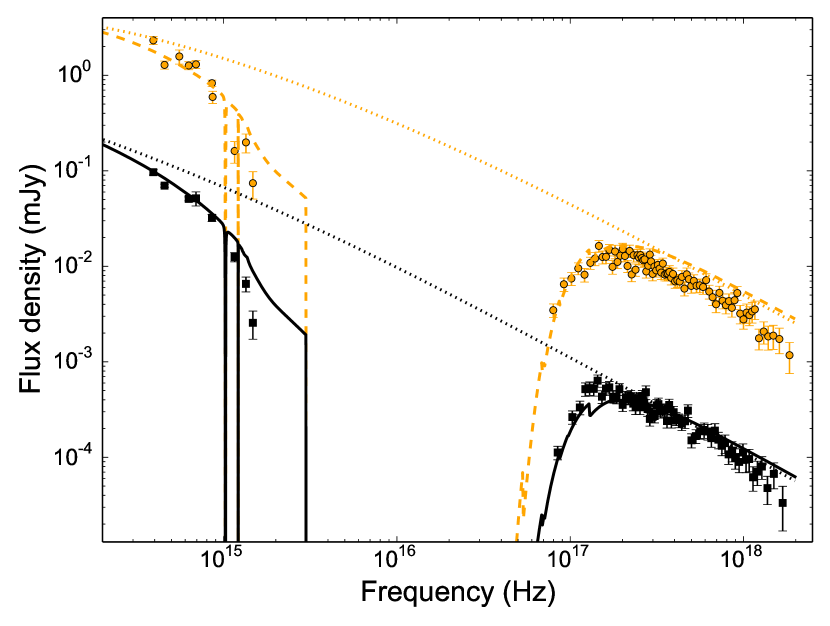
Figure 13.— Observed NIR to X-ray SED of the afterglow of GRB 100901A at 0.06 d (orange circles) and after the re-brightening (1.14 d; black squares), together with the best-fit ISM model (Section 6.2.2) including energy injection (Section 6.2.3) at 0.06 d (orange; dashed) and 1.14 d (black; solid). The data points and model at 0.06 d have been multiplied by a factor of 10. for clarity. The XRT SEDs at 1.14 d has been extrapolated from 3 d using the best-fit broken power law model to the XRT light curve (Figure 12; the correction factor is $\approx 4.5$). The optical data have been extrapolated using the joint best fit to the Swift/XRT and UVOT light curves (the corrections are small at $\lesssim 5\%$). The dotted curves indicate afterglow models with no extinction or IGM absorption. Note that the Swift/UVOT $uvw1$-, $uvw2$-, and $uvm2$-band data lie blueward of Ly-$\alpha$ in the rest-frame of the host galaxy ($1.0\times 10^{15}$ Hz in the observer frame), and are likely subject to significant IGM absorption. For this reason, we do not include these bands (or the Swift/UVOT White-band, not shown here) to constrain our afterglow model.

6.2.2 Forward shock model at $t\gtrsim 0.25$ d

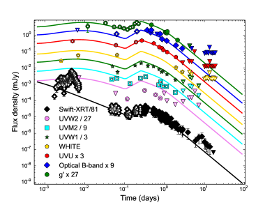
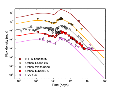
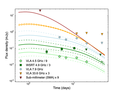
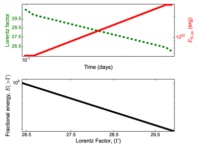
Figure 14.— X-ray, UV (top left), optical (top right), and radio (bottom left) light curves of GRB 100901A, with the full afterglow model (solid lines), including energy injection before 0.25 d. The X-ray data before 0.008 d exhibits strong flaring activity and we do not include these data in our analysis. The dashed envelopes around the radio light curves indicate the expected effect of scintillation at the $1\sigma$ level. The data indicated by open symbols are not used to determine the parameters of the forward shock (the MCMC analysis). Bottom right: blastwave Lorentz factor (green, dashed; upper sub-panel) and isotropic equivalent kinetic energy (red, solid; upper sub-panel) as a function of time, together with the energy distribution across ejecta Lorentz factors (black, solid; lower sub-panel) as determined from fitting the X-ray/UV/optical re-brightening at 0.36 d.

We employ our MCMC analysis to fit the multi-band data for GRB 100901A after $t\approx 0.25$ d. At the redshift of $z=1.408$, the UVOT White-, uvw1-, uvw2-, and uvm2-band data are affected by IGM absorption, and we do not include these bands in our analysis. The highest-likelihood ISM model (Figure 14) the parameters $p\approx 2.03$, $\epsilon_{\rm e}\approx 0.33$, $\epsilon_{B}\approx 0.32$, $n_{0}\approx 3.2\times 10^{-3}$ ${\rm cm}^{-3}$, $E_{\rm K,iso}\approx 3.0\times 10^{53}$ erg, $t_{\rm jet}\approx 0.96$ d, $A_{\rm V}\approx 0.09$ mag, and $F_{\nu,\rm host,r^{\prime}}\approx 4.1\,\mu$Jy, with a Compton $y$-parameter of $\approx 0.6$. The blastwave Lorentz factor is $\Gamma=15.9(t/1\,{\rm d})^{-3/8}$ and the jet opening angle is $\theta_{\rm jet}\approx 2.1\arcdeg$. The beaming-corrected kinetic energy is $E_{\rm K}\approx 2.1\times 10^{50}\,{\rm erg}$, while the beaming corrected $\gamma$-ray energy is $E_{\gamma}\approx 5\times 10^{49}$ erg (1–$10^{4}$ keV; rest frame). We plot histograms of the measured parameters in Figure 15 and correlation contours between the physical parameters in Figure 16, providing summary statistics from our MCMC analysis in Table 5.

In this model, the break frequencies at 1 d are located at $\nu_{\rm a}\approx 0.7$ GHz, $\nu_{\rm m}\approx 2\times 10^{12}$ Hz, and $\nu_{\rm c}\approx 9\times 10^{14}$ Hz, while the peak flux density is about 4.2 mJy at $\nu_{\rm m}$. The spectrum transitions from fast to slow cooling at about 350 s after the burst. The cooling frequency is located between the optical and X-rays and the jet break is before 1 d, both of which are expected from the basic analysis outlined above. The low value of $p$ is driven by the shallow measured decline in the X-rays following the jet break, and the resulting spectrum remains consistent with the optical-to-X-ray SED (Figure 13).

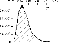
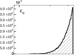
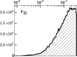
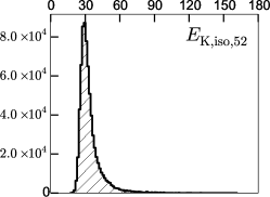
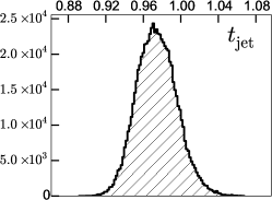
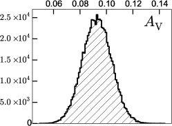
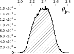
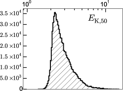
Figure 15.— Posterior probability density functions for the physical parameters for GRB 100901A in a constant density environment from MCMC simulations. We have restricted $E_{\rm K,iso,52}<500$, $\epsilon_{\rm e}<\nicefrac{{1}}{{3}}$, and $\epsilon_{\rm B}<\nicefrac{{1}}{{3}}$.

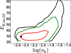
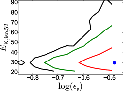
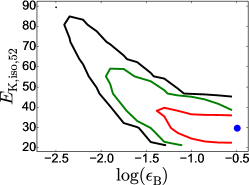
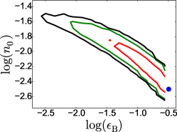
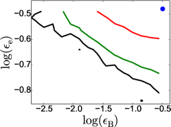
Figure 16.— 1$\sigma$ (red), 2$\sigma$ (green), and 3$\sigma$ (black) contours for correlations between the physical parameters, $E_{\rm K,iso}$, $n_{0}$, $\epsilon_{\rm e}$, and $\epsilon_{B}$ for GRB 100901A, in the ISM model from Monte Carlo simulations. We have restricted $\epsilon_{\rm e}<\nicefrac{{1}}{{3}}$ and $\epsilon_{\rm B}<\nicefrac{{1}}{{3}}$. See the on line version of this Figure for additional plots of correlations between these parameters and $p$, $t_{\rm jet}$, $\theta_{\rm jet}$, $E_{\rm K}$, $A_{\rm V}$, and $F_{\nu,\rm host,r^{\prime}}$.

6.2.3 Energy injection model

Taking the forward shock model described in Section 6.2.2 as a starting point, we find that the X-ray and UV/optical data before the re-brightening can be explained by a single period of energy injection between $0.105$ d and $\approx 0.26$ d:

$$E_{\rm K,iso}(t)=\begin{cases}E_{\rm K,iso,f},&t>t_{\rm 0}=0.26\,{\rm d}\\ E_{\rm K,iso,f}\left(\frac{t}{t_{\rm 0}}\right)^{1.88},&t_{1}=0.105\,{\rm d}<t<t_{\rm 0}\\ E_{\rm K,iso,f}\left(\frac{t_{1}}{t_{\rm 0}}\right)^{1.88},&t<t_{1}\\ \end{cases}$$ (5)

In this model, the energy increases by a factor of $\approx 5.5$ from $E_{\rm K,iso,i}\approx 5.4\times 10^{52}$ erg at 0.105 d to $E_{\rm K,iso,f}\approx 3.0\times 10^{53}$ erg at 0.26 d, corresponding to an injected energy fraction of $\approx 85\%$, while the Lorentz factor decreases from $\Gamma\approx 30$ to $\Gamma\approx 26$ over this period. In comparison, $E_{\gamma,\rm iso}\approx 8\times 10^{52}$ erg (Section 6.2.1). The value of $m\approx 1.88$ corresponds to $s\approx 14.4$ for $26\lesssim\Gamma\lesssim 30$.

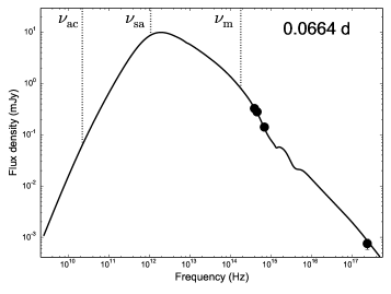
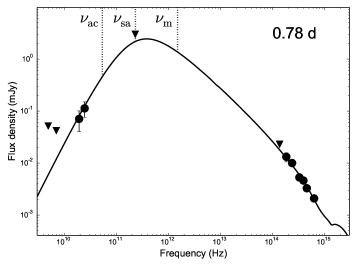
Figure 17.— Left: Observer-frame SED of the afterglow of GRB 120404A at 0.0664 d, together with the best fit model (spectrum 4 from GS02: black, solid). Right: The same as the left panel, but at 0.78 d. The radio detections with a steeply rising spectrum suggest that the self-absorption frequency is near or above the radio band, requiring a high circumburst density. Both SEDs are corrected for the effect of inverse Compton cooling, which is significant, with the Compton $y$-parameter $\approx 0.9$ during the fast cooling phase. We do not show the inverse Compton radiation, since even at its peak (near the Swift/XRT band), it is four orders of magnitude weaker than the synchrotron component. See Appendix A for a discussion of the inverse Compton effect in the context of modeling GRB afterglows.

6.3. GRB 120404A

6.3.1 GRB properties

GRB 120404A was detected and localized by the Swift BAT on 2012 April 04 at 12:51:02 UT (Stratta et al., 2012). The burst duration was $T_{90}=38.7\pm 4.1$ s, with a fluence of $F_{\gamma}=(1.6\pm 0.1)\times 10^{-6}$ erg cm^-2 (15–150 keV observer frame, Ukwatta et al., 2012). Swift and ground-based observatories detected an afterglow in the X-rays and UV/optical (Guidorzi et al., 2012; Xin et al., 2012b; Breeveld & Stratta, 2012; Gorbovskoy et al., 2012), as well as in the radio (Zauderer et al., 2012). Spectroscopic observations with Gemini-North yielded a redshift of $z=2.876$ (Cucchiara & Tanvir, 2012). The isotropic-equivalent $\gamma$-ray energy for this event is $E_{\gamma,\rm iso}=(9\pm 4)\times 10^{52}$ erg ($1$–$10^{4}$ keV, rest frame; Guidorzi et al. 2013).

This burst has been previously studied in detail by Guidorzi et al. (2013), who interpret the optical re-brightening starting around 800 s in their well-sampled, multi-band optical light curves as due to the passage of the characteristic synchrotron frequency, $\nu_{\rm m}$. They additionally invoke reverse shock emission to explain the flat ($t^{0.0\pm 0.1}$) portion of the optical light curve before the onset of the re-brightening. In the following, we propose an alternate model for the multi-band radio through X-ray light curves in the context of energy injection.

The X-ray light curve before 700 s can be modeled as a power law decay with $\alpha_{\rm X}\approx-2$. This light curve phase is likely part of the high latitude emission, and we ignore the data before 0.008 d in our analysis. The X-ray photon index at 0.12–0.24 d, $\Gamma_{X}=2.3\pm 0.3$ (Guidorzi et al., 2013), implying a spectrum, $F_{\nu}\propto\nu^{-1.3\pm 0.3}$, is consistent with the spectral slope between the optical $i^{\prime}$-band and the X-rays at 0.07 d, $\beta_{\rm opt-X}=-0.91\pm 0.04$, suggesting that the optical and X-ray bands are on the same segment of the afterglow SED, although the large uncertainty in $\beta_{\rm X}$ leaves open the possibility that $\nu_{\rm c}$ lies between the optical and X-rays. Additionally, the spectral slope within the optical ($B$- to $i^{\prime}$-band) is $\beta_{\rm opt}=-1.3\pm 0.2$ at 0.07 d, indicating that extinction is present. The spectral index between the 19.2 GHz and 24.5 GHz observations at 0.75 d is $\beta_{\rm radio}\approx 2$, which indicates that $\nu_{\rm a}$ is located above $24.5$ GHz at this time (Figure 17).

The optical $R$-band light curve declines as $t^{-1.9\pm 0.02}$ after 0.13 d, consistent with the X-ray decline rate of $t^{-1.8\pm 0.1}$ after 0.05 d. The steep decline of $\alpha\approx-2$ is indicative of a jet break before $\approx 0.1$ d. A broken power law fit to the $B$-band light curve results in the parameters $t_{\rm b}=(2.8\pm 0.4)\times 10^{-2}$ d, $F_{\nu,\rm B}(t_{\rm b})=252\pm 10\,\mu$Jy, $\alpha_{1}=1.74\pm 0.58$, $\alpha_{2}=-1.71\pm 0.17$, and $y=0.78\pm 0.43$, making this the earliest re-brightening episode of the four events studied in this paper.

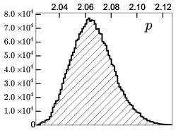
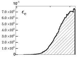
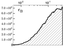
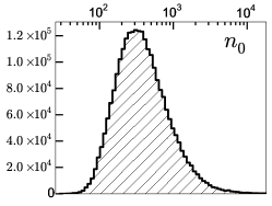
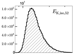
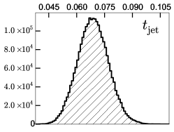
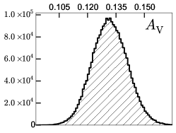
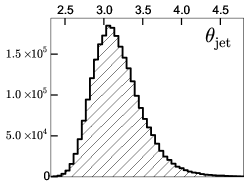
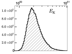
Figure 18.— Posterior probability density functions for the physical parameters for GRB 120404A in a constant density environment from MCMC simulations. We have restricted $E_{\rm K,iso,52}<500$, $\epsilon_{\rm e}<\nicefrac{{1}}{{3}}$, and $\epsilon_{\rm B}<\nicefrac{{1}}{{3}}$.

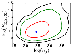
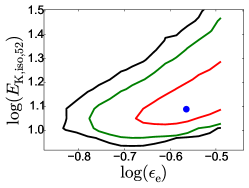
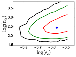
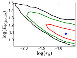
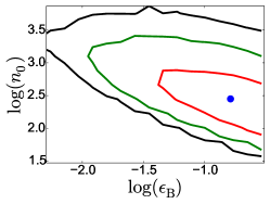
Figure 19.— 1$\sigma$ (red), 2$\sigma$ (green), and 3$\sigma$ (black) contours for correlations between the physical parameters, $E_{\rm K,iso}$, $n_{0}$, $\epsilon_{\rm e}$, and $\epsilon_{B}$ for GRB 120404A, in the ISM model from Monte Carlo simulations. We have restricted $E_{\rm K,iso,52}<500$, $\epsilon_{\rm e}<\nicefrac{{1}}{{3}}$, and $\epsilon_{\rm B}<\nicefrac{{1}}{{3}}$. See the on line version of this Figure for additional plots of correlations between these parameters and $p$, $t_{\rm jet}$, $\theta_{\rm jet}$, $E_{\rm K}$, and $A_{\rm V}$.

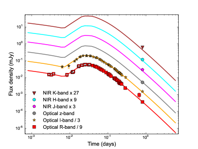
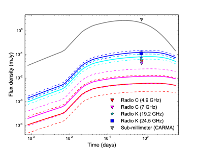
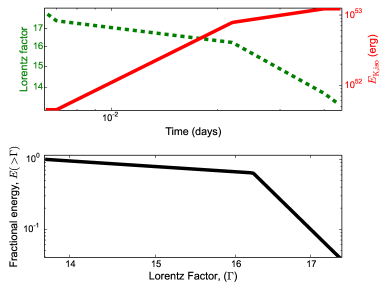
Figure 20.— X-ray, UV (top left), optical (top right), and radio (bottom left) light curves of GRB 120404A, with the full afterglow model (solid lines), including energy injection before 0.04 d. The X-ray data before 0.008 d is likely dominated by high-latitude prompt emission and we do not include these data in our analysis; the best fit power law to the X-ray data before 0.008 d added to the blastwave model is shown in the upper left panel (black, dashed). The dashed envelopes around the radio light curves indicate the expected effect of scintillation at the $1\sigma$ level. The data indicated by open symbols are not used to determine the parameters of the forward shock (the MCMC analysis). The $U$-band data are strongly affected by IGM absorption and are not included in the fit. Bottom right: blastwave Lorentz factor (green, dashed; upper sub-panel) and isotropic equivalent kinetic energy (red, solid; upper sub-panel) as a function of time, together with the energy distribution across ejecta Lorentz factors (black, solid; lower sub-panel) as determined from fitting the X-ray/UV/optical re-brightening at 0.04 d.

6.3.2 Forward shock model at $t\gtrsim 0.04$ d

We interpret the optical light curve peaks at around 2500 s as the end of a period of energy injection, after which the afterglow evolves according to the standard framework with a fixed energy, $E_{\rm K,iso,f}$. We use the data after 0.04 d for estimating the parameters of the blastwave shock and employ our MCMC tools described in Section 4 to model the afterglow after this time.

The parameters of our highest likelihood ISM model are $p\approx 2.06$, $\epsilon_{\rm e}\approx 0.27$, $\epsilon_{B}\approx 0.16$, $n_{0}\approx 2.8\times 10^{2}$ ${\rm cm}^{-3}$, $E_{\rm K,iso}\approx 1.2\times 10^{53}$ erg, $t_{\rm jet}\approx 6.6\times 10^{-2}$ d, and $A_{\rm V}\approx 0.13$ mag. The Compton $y$-parameter for this model is $\approx 0.9$. The blastwave Lorentz factor is $\Gamma=4.1(t/1\,{\rm d})^{-3/8}$ and the jet opening angle is $\theta_{\rm jet}\approx 3.1\arcdeg$. The beaming-corrected kinetic energy is $E_{\rm K}\approx 1.7\times 10^{50}\,{\rm erg}$, while the beaming corrected $\gamma$-ray energy is $E_{\gamma}\approx 1.2\times 10^{50}$ erg (1–$10^{4}$ keV; rest frame). The MCMC analysis yields an isotropic equivalent kinetic energy of $E_{\rm K,iso}$$=1.3^{+0.4}_{-0.2}\times 10^{53}$ erg, which is similar to the value of $1.9^{+0.7}_{-0.1}\times 10^{53}$ erg derived by Guidorzi et al. (2013). The high circumburst density of $\log{(n_{0})}=2.5^{0.4}_{-0.3}$ is also consistent with the value of $\log{(n_{0})}=2.4^{+0.02}_{-0.2}$ determined by Guidorzi et al. 2013), and is driven by the low flux density and steep spectrum in the radio. However, unlike Guidorzi et al. (2013), our low value of $p\approx 2.1$ allows us to match the NIR to optical SED and the normalization of the X-ray light curve. We note that the high circumburst density also results in a low cooling frequency: in our highest likelihood model $\nu_{\rm c}\ <\nu_{\rm a}$ and the spectrum remains in the fast cooling regime through the duration of the observations (spectrum 4 of Granot & Sari 2002), with $\nu_{\rm ac}\approx 5.9\times 10^{10}$ Hz, $\nu_{\rm sa}\approx 2.0\times 10^{11}$ Hz, $\nu_{\rm m}\approx 9.1\times 10^{11}$ Hz, and $\nu_{\rm c}\approx 6.3\times 10^{10}$ Hz at 1 d.

We plot the posterior density functions for the all parameters in Figure 18 and correlation contours in Figure 19; we list our measured values for the physical parameters in Table 5. In the wind and ISM models, light curves at all frequencies become indistinguishable following a jet break. Since the jet break occurs early, soon after the start of the data used for deriving the parameters of the blastwave, we expect a viable wind model to exist as well. We discuss this model in Appendix E.

6.3.3 Energy injection model

We model the light curves before $t_{0}=0.04$ d by injection of energy into the blastwave shock. We use the afterglow parameters for the highest-likelihood model (Section 6.3.2) as the final parameters following the end of energy injection, with $E_{\rm K,iso,f}=1.2\times 10^{53}$ erg. We find that the optical and X-ray light curves can be modeled well by two subsequent periods of energy injection, beginning at $t_{2}=7\times 10^{-3}$ d (Figure 20):

$$E_{\rm K,iso}(t)=\begin{cases}E_{\rm K,iso,f},&t>t_{\rm 0}=0.04\,{\rm d}\\ E_{\rm K,iso,f}\left(\frac{t}{t_{\rm 0}}\right)^{0.75},&t_{1}=2.2\times 10^{-2}\,{\rm d}<t<t_{\rm 0}\\ E_{\rm K,iso,f}\left(\frac{t_{1}}{t_{\rm 0}}\right)^{0.75}\left(\frac{t}{t_{1}}\right)^{2.5},&t_{2}=7.0\times 10^{-3}\,{\rm d}<t<t_{1}\\ E_{\rm K,iso,f}\left(\frac{t_{1}}{t_{\rm 0}}\right)^{0.75}\left(\frac{t_{2}}{t_{1}}\right)^{2.5},&t<t_{2}\\ \end{cases}$$ (6)

In this model, $E_{\rm K,iso}$ increases by a factor of $\approx 18$ from $4.4\times 10^{51}$ erg to $7.8\times 10^{52}$ erg between $7.0\times 10^{-3}$ d and $2.2\times 10^{-2}$ d, and then by $\approx 50\%$ to $E_{\rm K,iso,f}\approx 1.2\times 10^{53}$ erg between $2.2\times 10^{-2}$ d and $0.04$ d. Thus $\approx 95\%$ of the final kinetic energy is injected into the blastwave between $7.0\times 10^{-3}$ d and 0.04 d. In comparison, $E_{\gamma,\rm iso}\approx 10^{53}$ erg is similar to the final kinetic energy. The blastwave Lorentz factor decreases from $\Gamma\approx 17.4$ at $7.3\times 10^{-3}$ to $\Gamma\approx 16.2$ at $2.2\times 10^{-2}$ d, and then to $\Gamma\approx 13.7$ at the end of energy injection at $0.04$ d. The value of $m$ derived above corresponds to $s\approx 3.7$ for $13.7\lesssim\Gamma\lesssim 16.2$ and $s\approx 40$ for $16.2\lesssim\Gamma\lesssim 17.4$.

7. Discussion

7.1. Parameter distributions

We now turn to the question of how GRBs that exhibit simultaneous optical and X-ray re-brightening episodes compare with each other, and with events that do not exhibit such a feature. For this purpose, we use the compilation of measurements of $E_{\gamma}$, $\theta_{\rm jet}$, $E_{\rm K}$, and $n_{0}$ (or $A_{*}$) from the literature (Panaitescu & Kumar, 2002; Yost et al., 2003; Friedman & Bloom, 2005; Ghirlanda et al., 2007; Cenko et al., 2010, 2011) reported in Laskar et al. (2014). This sample includes GRBs from the pre-Swift era, as well as Swift and Fermi events.

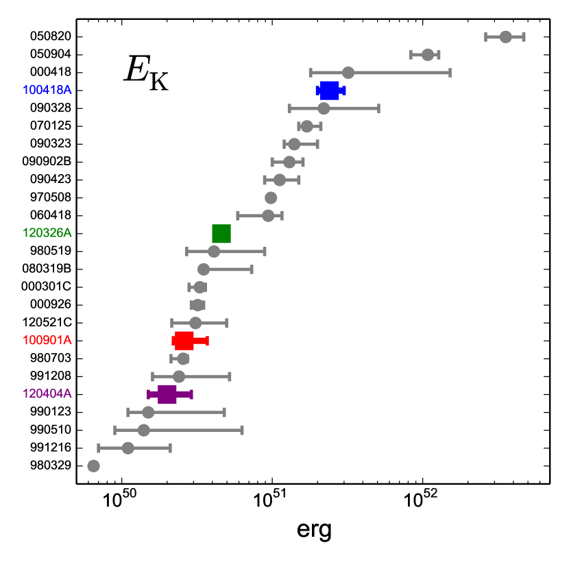
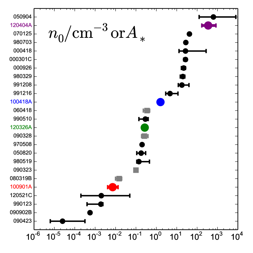
Figure 21.— Beaming-corrected kinetic energy (left) and circumburst density (right) for both ISM (black circles) and wind-like environments (grey squares). The four GRBs in our analysis 100418A (blue), 100901A (red), 120326AA (green), and 120404A (purple), do not appear distinct from the comparison sample (grey and black; Panaitescu & Kumar, 2002; Yost et al., 2003; Chandra et al., 2008; Cenko et al., 2010, 2011; Laskar et al., 2014).

The radio to X-ray observations of all four GRBs presented here can be fit by constant density ISM models. The best fit models yield densities from $\approx 3\times 10^{-3}$ to $\approx 3\times 10^{2}$ ${\rm cm}^{-3}$and final beaming-corrected kinetic energies from $\approx 2\times 10^{50}$ erg to $\approx 2\times 10^{51}$ erg, spanning the full range of values inferred from GRB afterglow modeling (Figure 21). We constrain the jet break time and hence the opening angle of the GRB jet in each case, and find $\theta_{\rm jet}\approx 2\,\arcdeg$–$21\,\arcdeg$, spanning the range inferred from the comparison sample.

The beaming-corrected $\gamma$-ray energies in the 1–$10^{4}$ keV rest frame energy band of the events in our sample range from $5\times 10^{49}$ erg to $1.3\times 10^{50}$ erg, while the median beaming corrected $\gamma$-ray energy of the comparison sample is $E_{\gamma}=\left(8.1^{+3.1}_{-4.1}\right)\times 10^{50}$ erg (95% confidence interval, Figure 22). Therefore, the observed values of $E_{\gamma}$ for the events in our sample are all smaller than the best estimate for the median of the comparison sample.

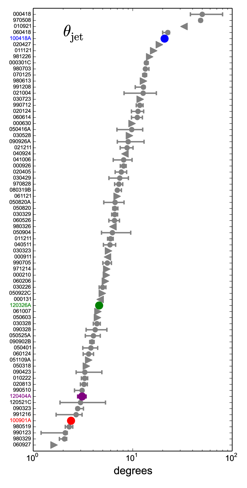
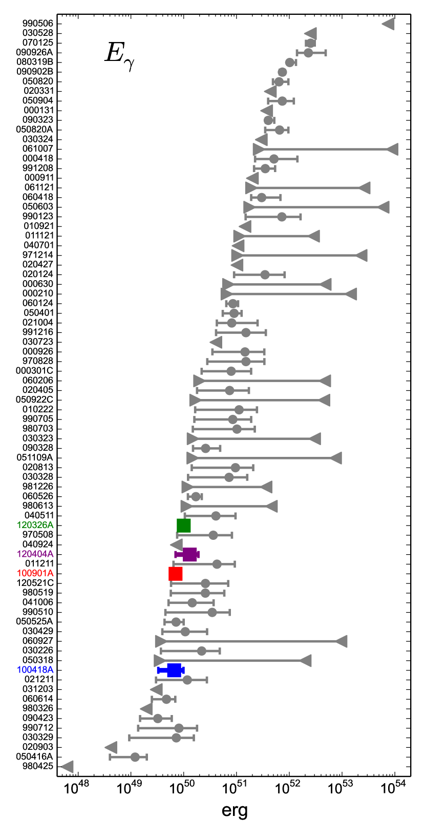
Figure 22.— Beaming-corrected $\gamma$-ray energy (left) and jet opening angle (right) for the events in our analysis, GRB 100418A (blue), 100901A (red), 120326AA (green), and 120404A (purple), together with a comparison sample of long GRBs (grey; Friedman & Bloom, 2005; Ghirlanda et al., 2007; Cenko et al., 2010, 2011; Laskar et al., 2014). The isotropic-equivalent $\gamma$-ray energy for GRB 050904 is taken from Amati et al. (2008), and for GRB 090423 from Salvaterra et al. (2009). The four GRBs exhibiting X-ray and optical re-brightening episodes do not appear distinct from the comparison sample in $\theta_{\rm jet}$, but appear to all reside at lower values of $E_{\gamma}$ than the median.

To further quantify this effect, we compute the radiative efficiency, $\eta\equiv E_{\rm K}/(E_{\gamma}+E_{\rm K})$ for each GRB and in the comparison sample. Since both $E_{\rm K}$  and $E_{\gamma}$ have associated uncertainties, while the expression for $\eta$ is non-linear in these two quantities, a proper accounting of the final uncertainty requires a Monte Carlo analysis. We generate $10^{5}$ Monte Carlo realizations of $E_{\rm K}$ and $E_{\gamma}$ for each burst, assuming a uniform distribution between the 1$\sigma$ error bars. We then compute and summarize the resulting distribution of $\eta$ using the median and $68\%$ credible intervals (Figure 23). We find that the GRBs in our sample have systematically lower radiative efficiencies. This is consistent with the energy injection scenario, if the prompt $\gamma$-ray radiation is dominated by emission from the fast-moving ejecta, while a significant amount of kinetic energy is carried by slow-moving ejecta.

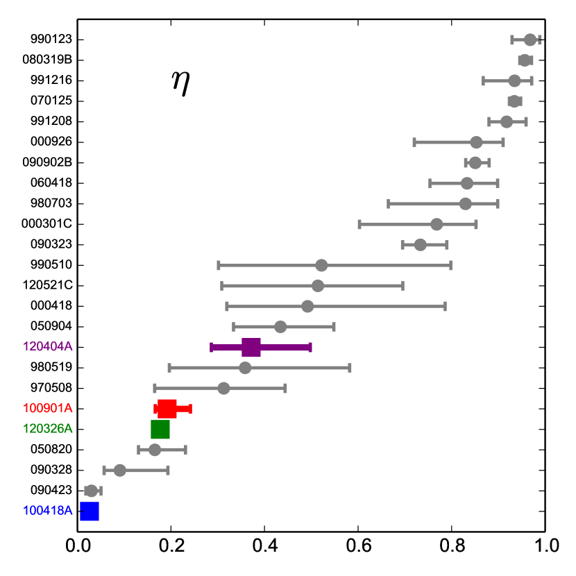
Figure 23.— Radiative efficiency, $\eta$ for the events in our analysis, GRB 100418A (blue), 100901A (red), 120326AA (green), and 120404A (purple), together with a comparison sample of long GRBs (grey; Friedman & Bloom, 2005; Ghirlanda et al., 2007; Cenko et al., 2010, 2011; Laskar et al., 2014), with 68% credible regions (error bars) about the median (points) computed from $E_{\rm K}$ and $E_{\gamma}$ using a Monte Carlo procedure. The four GRBs exhibiting X-ray and optical re-brightening episodes have lower radiative efficiencies than the median.

From this comparison, we conclude that events exhibiting simultaneous, multi-wavelength re-brightening episodes also span the same wide range of circumburst densities, jet opening angles, and beaming-corrected kinetic energies inferred from previous studies of events at $z\sim 1$ and $z\gtrsim 6$. However, the events reported here have smaller beaming-corrected $\gamma$-ray energies, and as a result lower radiative efficiencies than the comparison sample, suggesting that the prompt radiation is dominated by ejecta at high Lorentz factors, while the bulk kinetic energy is dominated by slow-moving ejecta at least in these cases.

7.2. Absence of reverse shock

When energy injection into the blastwave is caused by a distribution of ejecta Lorentz factors, the reverse shock (RS) from the initial interaction of the leading edge of the ejecta with the circumburst medium is expected to continue to propagate through the ejecta until the end of the period of energy injection (Sari & Mészáros, 2000). During the period of energy injection, the afterglow SED is expected to be composed of contributions from both forward (FS) and reverse (RS) shocks, each with its three characteristic frequencies and flux normalizations. The spectral characteristics of the two shocks are expected to be related by $F_{\nu,\rm max,RS}(t)=F_{\nu,\rm max,FS}(t)\times\Gamma(t)$, $\nu_{\rm m,RS}(t)=\nu_{\rm m,FS}(t)/\Gamma^{2}(t)$, and $\nu_{\rm c,RS}(t)=\nu_{\rm c,FS}(t)$, while the two self-absorption frequencies should be related by $\nu_{\rm a,RS}(t)=\nu_{\rm a,FS}(t)\times\Gamma^{\lambda}(t)$, where $\lambda=\nicefrac{{3}}{{5}}$ when both shocks are fast cooling and $\lambda=\nicefrac{{8}}{{5}}$ when both shocks are slow cooling. The reverse shock is expected to last through the period of energy injection, whereupon all ejecta have been decelerated to a common Lorentz factor, and the two shocks decouple in their subsequent evolution.

A calculation of the reverse shock SED based on the above considerations, together with the Lorentz factor of the blastwave at the end of the period of energy injection ($t_{\rm dec}$) and the SED of the forward shock at that time indicates that the reverse shock generically peaks around the millimeter band at $t_{\rm dec}$ (Sari & Mészáros, 2000). For GRB 100901A and 120404A, there are no data in the millimeter bands at the relevant time. For GRBs 120326A and 100418A where we have millimeter observations at $\approx t_{\rm dec}$, we find that the RS light curves over-predict the observations by factors of $\approx 2$–10. Additionally, the reverse shock would also contribute a flux density comparable to the forward shock in the X-rays and optical for all four events during energy injection, which would require suppressing the forward shock before the re-brightening by invoking even lower blastwave energies (and consequently requiring an even greater rate of energy injection) before the optical/X-ray peak. Thus the data are inconsistent with the presence of a strong reverse shock for these events.

We note that in our model there is a gap before the beginning of energy injection. If the energy injection is caused by a shell of material with a distribution of Lorentz factors (the ‘injective shell’) catching up with the initial shell (‘the impulsive shell’), then a long-lasting reverse shock in the injective shell is only expected when the two shells collide violently, with a relative Lorentz factor greater that the sound speed in the injective shell (Zhang & Mészáros, 2002). If the injective shell is released from the central engine at roughly the same time as the impulsive shell, the collision between the two will be mild, and a reverse shock will not occur. This appears to be the case for the GRBs studied here, suggesting that the shell collisions in these events exhibiting X-ray and UV/optical re-brightening episodes are gentle, resulting simply in a transfer of energy to the blastwave. Even more fundamentally, this implies that the shells are emitted at the same time from near the central engine and thus the engine need not be on during the re-brightening episode.

7.3. Energy injection: a ubiquitous phenomenon?

The phenomenon of short-lived plateaus at an early time is ubiquitous in Swift/XRT afterglow light curves (Liang et al., 2007). Using a complete sample of Swift/XRT light curves through 2010, Margutti et al. (2013) find about $37\%$ of long-duration GRBs exhibit a shallow decay phase, with $-1\lesssim\alpha\lesssim 1$. If these plateaus are caused by injection of energy into the forward shock, the events with X-ray/optical re-brightenings discussed in this paper might be the extreme tail of a distribution in energy injection factor, duration or rate. A rigorous exploration of these possibilities requires multi-wavelength fits to the data, but such data are generally not available. We therefore compute energy injection fractions based on the X-ray light curves alone, and compare the results for the objects where we do have multi-wavelength observations as reported in this paper.

Margutti et al. (2013) measured the timing of X-ray plateaus in Swift/XRT light curves and quantified them by their start time, $t_{1}$, end time, $t_{2}$, and rise rate during the plateau phase, $\alpha$. For our X-ray plateau analysis, we select the 96 events in their study where the reported uncertainty in $\alpha$ is $<0.3$. We repeat their light curve decomposition analysis on the X-ray light curves of GRB 120326A and GRB 120404A (which are not included in their sample), and find $t_{1}=5.7\times 10^{-3}$ d, $t_{2}=0.62$ d, and $\alpha=0.27\pm 0.03$, for GRB 120326A and $t_{1}=9.8\times 10^{-3}$ d, $t_{2}=2.9\times 10^{-2}$ d, and $\alpha=0.76\pm 0.23$ for GRB 120404A.

We define the plateau duration, $\Delta T\equiv t_{2}-t_{1}$ and the fractional duration, $\xi\equiv(t_{2}-t_{1})/(t_{2}+t_{1})\in[0,1)$. Note that $\xi\to 1$ when $t_{2}\gg t_{1}$, which corresponds to the case that the plateau lasts much longer than its onset time. Margutti et al. (2013) computed the start time of the plateau using the intersection of the steep decay phase with the best fit plateau model; hence they do not report an error on this quantity. We can estimate the uncertainty on $\xi$ using $\sigma_{\xi}=\sigma_{t_{2}}\partial\xi/\partial t_{2}=2t_{1}\sigma_{t_{2}}/(t_{1}+t_{2})^{2}$, which is dimensionless as desired.

Assuming the X-ray band is located above the cooling frequency for all cases (which is indeed the case for the five events considered in detail here), and that $p=2$, we can compute an effective energy injection rate, $E\propto t^{m}$, where $m=\alpha+1$ is the rate required to bring the measured light curve slope to $\alpha$ from the theoretically-expected value of $t^{(2-3p)/4}\propto t^{-1}$ for no energy injection. For the sake of simplicity and uniformity, we use $p=2$ even where we have other measurements of $p$, such as for the events reported in this paper. The ratio of the energy at the end of the plateau phase to the energy at the beginning of the plateau phase is then given by $\Upsilon\equiv E_{2}/E_{1}=(t_{2}/t_{1})^{m}$.

We plot the plateau fractional duration, $\xi$ against the plateau slope, $\alpha$ in Figure 24, scaling the area of the symbols by $\Upsilon$. The slopes during the plateau phase range from $\alpha\approx-1$ to $\approx 1.8$. As evident from the kernel density estimate of $\alpha$, most light curves exhibit a gentle decay during the plateau phase (Figure 24). However, all four events in our sample are exceptions to this rule. These four events also exhibit the greatest rise in their plateau phase light curves for a given normalized duration, $\xi$. Two out of these four (GRBs 120326A and 100418A) have the largest fractional changes in the kinetic energy of the entire sample of 98 events. These are also the events with the largest value of $\xi$ in our sample. For GRB 120404A, we note that the X-ray light curve around the peak of the re-brightening is missing due to a Swift orbital gap. Therefore any results that rely solely on the X-ray data of this burst underestimate the value of $\alpha$ and the fraction of energy injection relative to the multi-wavelength analysis we carried out in Section 6.3.3.

In Figure 25 we plot the ratio of final to initial energy, $\Upsilon$ against the normalized plateau duration, $\xi$, scaling the radius of the symbols by $\alpha$. We find that for a given (normalized) plateau duration, the events in our sample have the largest fractional change in blastwave kinetic energy during the plateau phase. At the same time, they also possess the steepest rise rates in the sample, which is simply indicative of our selection criteria for inclusion in the present analysis. Finally, these events have the shortest normalized plateau durations for a given fractional change in energy. Together, these observations suggest that a large amount of injected energy is not sufficient to cause simultaneous -ray/optical re-brightenings, but that it must be done in a relatively small amount of time, and thus that the defining characteristic of these events is a high rate of energy injection. Physically, this translates to a steep distribution of ejecta Lorentz factors over a small range of $\Gamma$. Hascoet et al. (2015) recently suggested that the interaction of low-Lorentz factor ejecta with the reverse shock can explain flares in the X-ray light curves. Our observations provide supporting evidence for this hypothesis in the form of significant ejecta energy down to the requisite low Lorentz factors, $\Gamma\sim 10$.

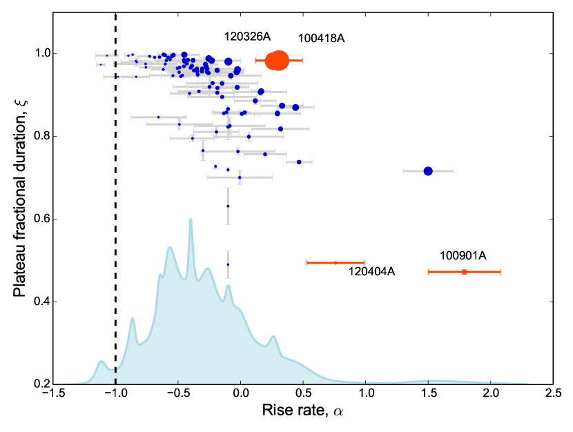
Figure 24.— The fractional duration of X-ray plateaus from Margutti et al. (2013) as a function of the light curve rise rate, $\alpha$ (with the convention $F\propto t^{\alpha}$). Errors in both directions are computed according to the formulas described in section 7.3. The vertical dashed black line indicates the canonical light curve decay of $\alpha\approx-1$ expected for $p\approx 2$. 21% of events with plateaus exhibit re-brightenings ($\alpha>0$). Events analyzed in this paper are shown in red. The area of each symbol is linearly proportional to the ratio of the energy at the end to that at the beginning of the plateau phase, $\Upsilon$. The blue point at $\alpha\approx-1.5$ is GRB 081028, which also exhibits an X-ray/optical re-brightening; however, this event does not have radio data and we therefore exclude it from our multi-wavelength analysis. A probability density function of the distribution of $\alpha$ (computed from a kernel density estimate using $\sigma_{\alpha}$ as a varying kernel bandwidth) is shown in cyan.

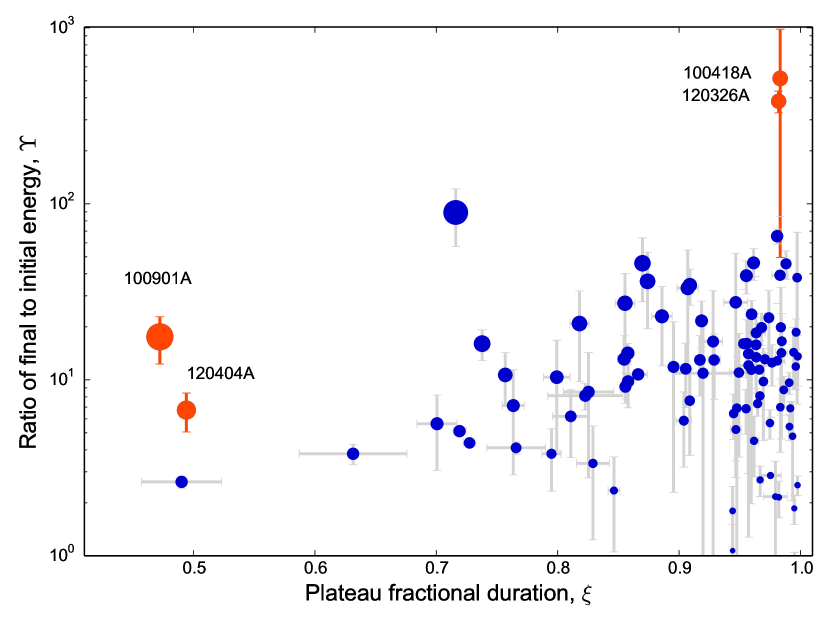
Figure 25.— The ratio of energy at the end to that at the beginning of the plateau phase in X-ray light curves of 96 events from Margutti et al. (2013), as well as GRBs 120326A and 120404A from our analysis, as a function of the plateau fractional duration, $\xi$, with error bars computed according to the prescription in section 7.3. The size of the symbols is scaled to a measure of the light curve rise rate during the plateau decay phase, $\alpha$, with the radius of the symbols proportional to $\alpha+1.5$. Larger symbols denote a greater departure from a canonical light curve decay of $\alpha\approx-1$, indicating greater rates of energy injection during the plateau phase.

7.4. Energetics

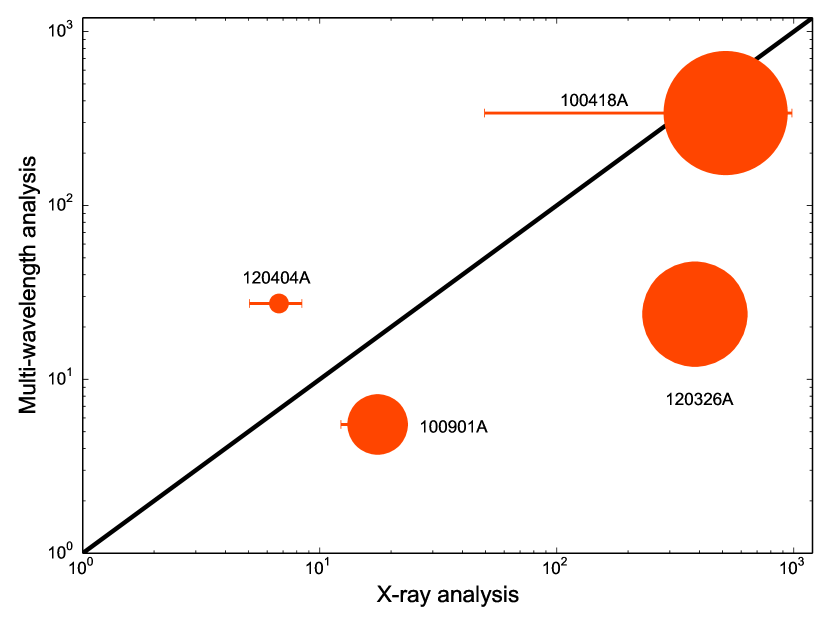
Figure 26.— Ratio of final energy to the energy prior to the first injection episode from the multi-wavelength analysis (y-axis) compared to the ratio of the energy at the end to that at the start of the ‘plateau phase’, $\Upsilon$, computed in section 7.3 for the five events in our sample, together with the 1:1 line (solid, black). The area of the symbols is linearly proportional to the physical duration of the plateaus, $t_{2}-t_{1}$.

Having compared the plateau duration, light curve rise rate, and injected energy fraction for our sample with a complete sample of Swift events using the X-ray data alone, we now turn to an analysis of the results from our multi-wavelength energy injection modeling in this context. In Figure 26 we plot the fractional change in energy determined from multi-wavelength modeling against the fractional change in energy, $\Upsilon$, inferred from the X-ray-only analysis in section 7.3 for the four events in our sample. We scale the area of the symbols with the plateau physical duration, $t_{2}-t_{1}$. As expected, events with longer plateau durations have greater estimated energy injection fractions both from the X-ray analysis and from the full multi-wavelength study. The fractional change in energy from the X-ray analysis is higher than inferred from the full model for three out of four cases. This is due to the typically lower value of $m$ from the X-ray-only analysis compared to the full model. Ultimately, this can be traced to the fitting procedure: Margutti et al. (2013) fit a sum of a steep decay and a rising light curve, the sum of which results in the X-ray plateau, whereas we do not subtract fits to the steep decay phase from the X-ray light curve prior to our multi-band modeling. In the case of GRB 120326A, where the X-ray analysis over-estimates $\Upsilon$ by an order of magnitude, the variance between the two techniques is due to differences in the plateau start time ($4.3\times 10^{-2}$ d for the multi-wavelength analysis, compared to $5.7\times 10^{-3}$ d in the X-ray analysis). Based on this comparison, we conclude that a determination of $\Upsilon$ using the X-ray data alone yields a reasonable estimate of the energy injection factor on average, but that multi-wavelength modeling is essential to obtain the full picture.

8. Summary and Conclusions

Plateaus and re-brightening episodes are frequent in GRB afterglow X-ray light curves. However, X-ray data by themselves provide only a limited understanding of the physical processes underlying these unexpected phenomena. We perform a thorough multi-wavelength study of all long-duration GRBs through 2012 featuring simultaneous X-ray, and UV/Optical re-brightenings and that have radio detections, using a Markov Chain Monte Carlo analysis and a physical afterglow model. Our analysis yields the first set of models that explain the multi-wavelength afterglows for all of these events with the same unifying principle. In all cases, the afterglow light curves can be modeled with a standard forward shock model following the re-brightening episode, an ISM density profile, and a jet break. From our multi-wavelength analysis, we find that the circumburst densities, jet opening angles, and beaming-corrected kinetic energies for these events span the full range described by typical GRBs at $z\sim 1$ and $z\gtrsim 6$.

We explore a range of possible models to understand the re-brightenings, including the onset of the afterglow, off-axis viewing geometry, and continuous energy injection. We are able to rule out the afterglow onset and off-axis jets, and find instead that injection of energy into the blastwave (the so-called ‘refreshed-shock’ scenario) provides a good explanation for all events. We interpret energy injection in the framework of the stratified Lorentz factor model, and find that our measured energy injection rates always obey the theoretical constraints relating the rate of injection and the distribution of ejecta Lorentz factors in the ISM model.

We perform the first measurement of the ejecta Lorentz factor distribution index, $s$, and find $s\approx 3$–$40$, suggesting that a large amount of kinetic energy resides in the slowest-moving ejecta. This is supported by low radiative efficiencies for the events in our sample, indicating that the $\gamma$-ray radiation is dominated by ejecta at high Lorentz factors, while the kinetic energy is dominated by slower-moving ejecta. We note that keeping the injection rates simple power laws allows us to directly convert the injection rate to a Lorentz factor distribution index, but the true injection rate and also the true Lorentz factor distribution is likely to be a smoother function of time and Lorentz factor, respectively.

Finally, using a compilation of X-ray plateaus in GRB afterglows, we present a comparative discussion of this interesting sub-population of GRBs. We find that the phenomenon of energy injection is ubiquitous is long-duration GRBs, with re-brightening episodes likely simply extreme injection events. In future work, we aim to fit the light curves before the re-brightening episodes in a statistical sense, allowing us to estimate uncertainties on the rate and duration of the energy injection episodes. At the same time, radio monitoring of Swift events exhibiting re-brightening episodes will be crucial in multi-wavelength modeling of this interesting class of GRBs, while ALMA observations will irrefutably establish the presence or absence of reverse shocks, laying to rest the question of whether the energy injection process is violent or gentle.

Appendix A Inverse Compton Correction

The synchrotron photons produced in the GRB blastwave can Compton-scatter off the shock-accelerated relativistic electrons in the blastwave, producing a Comptonized spectrum at high energies (Panaitescu & Mészáros, 1998; Wei & Lu, 1998; Totani, 1998; Chiang & Dermer, 1999; Dermer et al., 2000a, b; Panaitescu & Kumar, 2000; Blandford & McKee, 1977; Sari & Esin, 2001). We compute the IC spectrum by directly integrating the synchrotron spectrum over the electron Lorentz factor distribution (back-calculated from the synchrotron spectrum) using equation A2 in Sari & Esin (2001). We find that IC emission contributes negligible flux compared to synchrotron radiation and we ignore this component in our analysis. However, the IC mechanism can provide a significant source of cooling for the shock-accelerated electrons and thereby dominate the total cooling rate, even when IC emission itself is not directly observable (Sari et al., 1996; Sari & Esin, 2001; Zhang et al., 2007). This effects the synchrotron cooling frequency, as well as the self-absorption frequency (when $\nu_{\rm c}<\nu_{\rm m}$). Thus IC cooling should be taken into account when computing SEDs and light curves for the synchrotron component.

The importance of IC cooling is determined by the Compton $y$-parameter,

$$Y=\frac{-1+\sqrt{1+4\eta\epsilon_{\rm e}/\epsilon_{B}}}{2},$$ (A1)

where $\eta$ is the fraction of energy that has been radiated away due to synchrotron and IC radiation, such that $\eta=1$ during fast cooling and $\eta=\left(\nu_{\rm c}/\nu_{\rm m}\right)^{-(p-2)/2}$ during slow cooling (Sari & Esin, 2001). Writing $\nu_{\rm c}=\nu_{\rm c}^{\prime}(1+Y)^{-2}$, where $\nu_{\rm c}^{\prime}$ is the cooling frequency of the synchrotron SED not corrected for IC cooling, we have

$$\eta = \left[\frac{\nu_{\rm c}^{\prime}(1+Y)^{-2}}{\nu_{\rm m}}\right]^{-(p-2)/2}=\left(\frac{\nu_{\rm c}^{\prime}}{\nu_{\rm m}}\right)^{-(p-2)/2}(1+Y)^{p-2}$$ (A2)

$$= H\left[\frac{1+\sqrt{1+4\eta\epsilon_{\rm e}/\epsilon_{B}}}{2}\right]^{p-2},$$

where $H=(\nu_{\rm c}^{\prime}/\nu_{\rm m})^{-(p-2)/2}$ is independent of $\eta$. We therefore obtain the following implicit equation for $\eta$,

$$f(\eta)\equiv\eta-H\left[\frac{1+\sqrt{1+4\eta\epsilon_{\rm e}/\epsilon_{B}}}{2}\right]^{p-2}=0,$$ (A3)

which can be solved numerically using (for instance) the Newton-Raphson method. Finally, the effect of IC cooling can be accounted for by scaling the spectral break frequencies and flux densities of the synchrotron spectrum by the appropriate powers of $1+Y$ (Granot & Sari, 2002). For convenience, we summarize these scaling relations in Table 9.

Table 9Inverse Compton Corrections to Spectral Break Frequencies

Spectral Break	Break Frequency	Break type	Frequency scaling	Flux density scaling
1	$\nu_{\rm sa}$	Self-absorption	$(1+Y)^{0}$	$(1+Y)^{0}$
2	$\nu_{\rm m}$	Characteristic	$(1+Y)^{0}$	$(1+Y)^{0}$
3	$\nu_{\rm c}$	Cooling	$(1+Y)^{-2}$	$(1+Y)^{p-1}$
4	$\nu_{\rm m}$	Characteristic	$(1+Y)^{0}$	$(1+Y)^{0}$
5	$\nu_{\rm sa}$	Self-absorption	$(1+Y)^{0}$	$(1+Y)^{0}$
6	$\nu_{\rm sa}$	Self-absorption	$(1+Y)^{\frac{-2}{p+5}}$	$(1+Y)^{\frac{-5}{p+5}}$
7	$\nu_{\rm ac}$	Self-absorption	$(1+Y)^{-3/5}$	$(1+Y)^{-6/5}$
8	$\nu_{\rm sa}$	Self-absorption	$(1+Y)^{-1/3}$	$(1+Y)^{-5/6}$
9	$\nu_{\rm m}$	Characteristic	$(1+Y)^{0}$	$(1+Y)^{-1}$
10	$\nu_{\rm sa}$	Self-absorption	$(1+Y)^{1}$	$(1+Y)^{1}$
11	$\nu_{\rm c}$	Cooling	$(1+Y)^{-2}$	$(1+Y)^{0}$

Appendix B A Wind Model for GRB 120326A

In Sections 5.1 we discussed the ISM model for GRB 120326A. We now consider the possibility of a wind-like circumburst environment.

The best fit model in a wind environment requires $p\approx 2.52$, $\epsilon_{\rm e}\approx 4.9\times 10^{-2}$, $\epsilon_{B}\approx 1.0\times 10^{-2}$, $A_{*}\approx 7.0\times 10^{-2}$, $E_{\rm K,iso}\approx 3.6\times 10^{54}$ erg, $t_{\rm jet}\approx 19$ d, $A_{\rm V}\approx 0.46$ mag, and $F_{\nu,\rm host,r^{\prime}}\approx 1.6\,\mu$Jy. This model transitions from fast cooling to slow cooling at $3.5\times 10^{-2}$ d. The spectral break frequencies at 1 d are located at $\nu_{\rm a}\approx 6.8\times 10^{8}$ Hz, $\nu_{\rm m}\approx 2.2\times 10^{14}$ Hz, and $\nu_{\rm c}\approx 4.2\times 10^{15}$ Hz. The peak of the spectrum ($f_{\nu}$) is at $\nu_{\rm m}$, with a flux density of $\approx 23$ mJy.

From our MCMC simulations, we find $p=2.52\pm 0.02$, $E_{\rm K,iso}=\left(3.1^{+0.9}_{-0.5}\right)\times 10^{54}$ erg, $A_{*}=\left(4.8^{+3.3}_{-2.5}\right)\times 10^{-2}$, $\epsilon_{\rm e}=\left(4.1^{+1.3}_{-1.2}\right)\times 10^{-2}$, $\epsilon_{B}=\left(2.8^{+9.4}_{-2.1}\right)\times 10^{-2}$, and $t_{\rm jet}=18.7^{3.1}_{-2.9}$ d. Using the relation $\theta_{\rm jet}=0.17\left(2\frac{t_{\rm jet}*A_{*}}{(1+z)E_{\rm K,iso,52}}\right)^{1/4}$ for the jet opening angle (Chevalier & Li, 2000), and the distributions of $E_{\rm K,iso}$, $n_{0}$, and $t_{\rm jet}$ from our MCMC simulations (Figure 27), we find $\theta_{\rm jet}=2.1^{+0.2}_{-0.3}$ degrees. Applying the beaming correction, $E_{\gamma}=E_{\gamma,\rm iso}(1-\cos{\theta_{\rm jet}})$, we find $E_{\gamma}=(2.1\pm 0.3)\times 10^{49}$ erg. The beaming-corrected kinetic energy is much larger, $E_{\rm K}=\left(2.0^{+1.0}_{-0.6}\right)\times 10^{51}$ erg. In this model, $\nu_{\rm a}$ falls below $10^{10}$ Hz at $1.7\times 10^{-2}$ d and is therefore not probed by any of the radio data. Consequently, the model exhibits a degeneracy in its parameters due to to the unknown value of $\nu_{\rm a}$ (Figure 28). This high value of $E_{\rm K}$ also implies a low radiative efficiency, $\eta_{\rm rad}\equiv E_{\gamma}/(E_{\rm K}+E_{\gamma})\approx 1\%$.

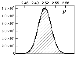
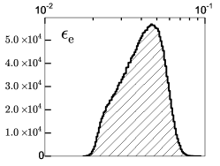
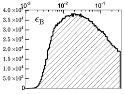
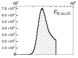
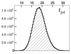
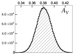
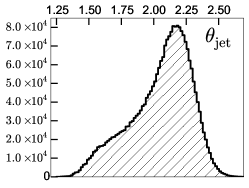
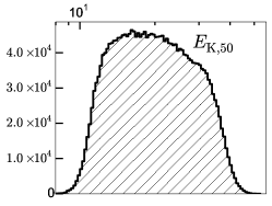
Figure 27.— Posterior probability density functions for the physical parameters for GRB 120326A in the wind model from MCMC simulations. We have restricted $E_{\rm K,iso,52}<500$, $\epsilon_{\rm e}<\nicefrac{{1}}{{3}}$, and $\epsilon_{\rm B}<\nicefrac{{1}}{{3}}$.

We now investigate the effect of energy injection in causing an X-ray/UV/optical re-brightening. The X-ray light curve during the re-brightening is located above the cooling frequency. In the wind model, the flux density above $\nu_{\rm c}$ is $F_{\nu>\nu_{\rm c}}\propto E_{\rm K,iso}^{(2+p)/4}t^{(2-3p)/4}$ (Granot & Sari, 2002). For $p=2.5$, this reduces to $F_{\nu>\nu_{\rm c}}\propto E_{\rm K,iso}^{1.13}t^{-1.38}$. During energy injection, $E\propto t^{m}$, such that $F_{\nu>\nu_{\rm c}}\propto t^{1.13m-1.38}$. The steep rise ($\alpha_{1}=0.85\pm 0.19$; Section 3.1) requires $m=2.0\pm 0.2$. However $0\leq m<1$ is bounded (Section 5.2.4), which implies that in this model, energy injection due to a distribution of ejecta energy to lower Lorentz factors can not cause the X-ray flux to rise with time.

Relaxing the requirement $m<1$, our best solution for the multi-wavelength re-brightening for an energy injection model requires two periods of energy injection. In the first episode between $1.7\times 10^{-3}$ d and $2.5\times 10^{-2}$ d, $E_{\rm K,iso}$ increases as $t^{0.5}$ growing by a factor of $3.9$ from $1.6\times 10^{51}$ erg to $6.2\times 10^{51}$ erg. In the second episode, $E_{\rm K,iso}\propto t^{2.3}$ from $2.5\times 10^{-2}$ d to 0.4 d, further increasing by a factor of over 2000 to its final value of $E_{\rm K,iso}\approx 3.6\times 10^{54}$ erg in this period. The resulting light curves, which are optimized to match the UV and optical re-brightening, cannot reproduce the X-ray light curve prior to the re-brightening (a shallower rise in the X-rays in the ISM model was achieved by placing $\nu_{\rm m}$ between the optical and X-rays). Due to the extremely large injected energy coupled with the fact that the steep rise in the optical violates the bounds on $m$, the wind model is a less attractive solution for the multi-wavelength afterglow of GRB 120326A.

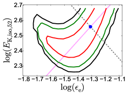
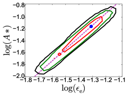
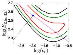
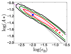
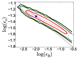
Figure 28.— 1$\sigma$ (red), 2$\sigma$ (green), and 3$\sigma$ (black) contours for correlations between the physical parameters, $E_{\rm K}$, $A_{*}$, $\epsilon_{\rm e}$, and $\epsilon_{B}$ for GRB 120326A, in the wind model from Monte Carlo simulations. We have restricted $E_{\rm K,iso,52}<500$, $\epsilon_{\rm e}<\nicefrac{{1}}{{3}}$, and $\epsilon_{\rm B}<\nicefrac{{1}}{{3}}$. The dashed grey lines indicate the expected relations between these parameters when $\nu_{\rm a}$ is not fully constrained: $E_{\rm K,iso}\propto A_{*}^{-1/2}$, $E_{\rm K,iso}\propto\epsilon_{\rm e}^{-1}$, $A_{*}\propto\epsilon_{\rm e}^{2}$, $E_{\rm K,iso}\propto\epsilon_{B}^{1/3}$, $A_{*}\propto\epsilon_{B}^{-2/3}$, and $\epsilon_{\rm e}\propto\epsilon_{B}^{-1/3}$, normalized to pass through the highest-likelihood point (blue dot), while the dotted magenta lines indicate expected relations for changes the value of $\nu_{\rm c}$: $E_{\rm K,iso}\propto A_{*}^{1/2}$, $E_{\rm K,iso}\propto\epsilon_{\rm e}$, $A_{*}\propto\epsilon_{\rm e}^{2}$, $E_{\rm K,iso}\propto\epsilon_{B}^{-1/5}$, $A_{*}\propto\epsilon_{B}^{-2/5}$, and $\epsilon_{\rm e}\propto\epsilon_{B}^{-1/5}$. $\nu_{\rm a}$ falls below the radio band before any radio observations took place, and is therefore unconstrained. $\nu_{\rm c}$ lies between the optical and X-ray bands and is better constrained; the correlations between the parameters along the lines of varying values of $\nu_{\rm c}$ are likely indicative of the strong changes (over two orders of magnitude) in the Compton $y$-parameter along these curves. See the on-line version of this Figure for additional plots of correlations between these parameters and $p$, $t_{\rm jet}$, $\theta_{\rm jet}$, $E_{\rm K}$, $A_{\rm V}$, and $F_{\nu,{\rm host,r^{\prime}}}$.

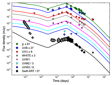
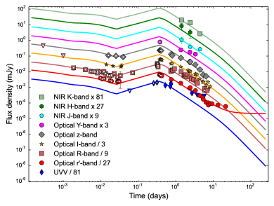
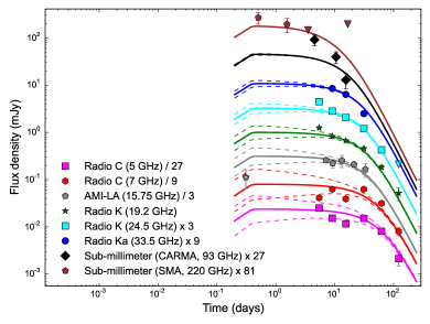
Figure 29.— X-ray, UV (top left), optical (top right), and radio (bottom left) light curves of GRB 120326A in the wind scenario, with the full afterglow model (solid lines), including energy injection before 0.4 d.

Appendix C A Wind Model for GRB 100418A

We apply our MCMC analysis described in Section 6.1.2 to explore afterglow models with a wind-like circumburst environment for GRB 100418A. The parameters of the highest-likelihood model are $p\approx 2.1$, $\epsilon_{\rm e}\approx 0.33$, $\epsilon_{B}\approx 0.33$, $A_{*}\approx 0.15$, $E_{\rm K,iso}\approx 4.0\times 10^{51}$ erg, and $F_{\nu,\rm host,White}\approx 2.3\,\mu$Jy, with negligible extinction. This model transitions from fast to slow cooling at $1.5$ d. The spectral break frequencies at 1 d are located at $\nu_{\rm ac}\approx 5.8$ GHz, $\nu_{\rm sa}\approx 32$ GHz, $\nu_{\rm c}\approx 6.4\times 10^{11}$ Hz, and $\nu_{\rm m}\approx 3.6\times 10^{12}$ Hz at 1 d, with $F_{\rm max}\approx 50$ mJy at $\nu_{\rm c}$ at 1 d and a Compton $y$-parameter of 0.6.

Like in the ISM model, the optical and X-ray bands are located above both $\nu_{\rm m}$  and $\nu_{\rm c}$. This model does not require a jet break, and we find $t_{\rm jet}\gtrsim 140$ d. Thus we cannot constrain $\theta_{\rm jet}$ in this model, nor correct $E_{\gamma,\rm iso}$ or $E_{\rm K,iso}$ for beaming. The summary statistics from our MCMC simulations are $p=2.12\pm 0.01$, $E_{\rm K,iso}=(4.2\pm 0.4)\times 10^{51}$ erg, $A_{*}=0.16^{+0.008}_{-0.006}$, $\epsilon_{\rm e}=0.328^{+0.004}_{-0.009}$, and $\epsilon_{B}=0.31^{+0.03}_{-0.02}$. We plot histograms of the posterior density functions for these parameters in Figure 30 and present contours of the joint posterior density for the physical parameters $A_{*}$, $E_{\rm K,iso}$, $\epsilon_{\rm e}$, and $\epsilon_{B}$ in Figure 31.

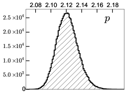
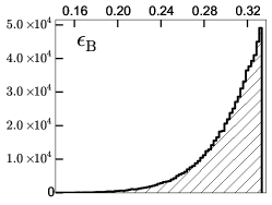
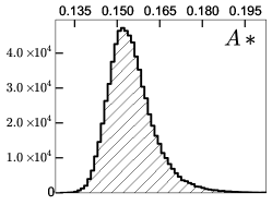
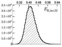
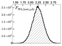
Figure 30.— Posterior probability density functions for the physical parameters for GRB 100418A in a wind environment from MCMC simulations. We have restricted $E_{\rm K,iso,52}<500$, $\epsilon_{\rm e}<\nicefrac{{1}}{{3}}$, and $\epsilon_{\rm B}<\nicefrac{{1}}{{3}}$. The last panel corresponds to the flux density of the host galaxy in the Swift/White band.

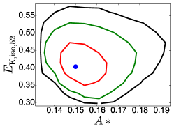
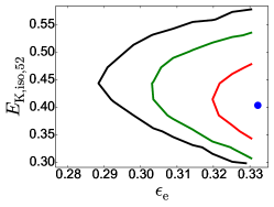
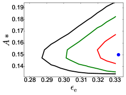
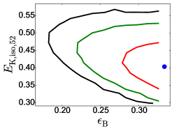
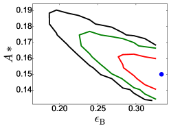
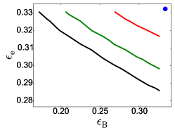
Figure 31.— 1$\sigma$ (red), 2$\sigma$ (green), and 3$\sigma$ (black) contours for correlations between the physical parameters, $E_{\rm K,iso}$, $n_{0}$, $\epsilon_{\rm e}$, and $\epsilon_{B}$ for GRB 100418A, in the wind model from Monte Carlo simulations. We have restricted $E_{\rm K,iso,52}<500$, $\epsilon_{\rm e}<\nicefrac{{1}}{{3}}$, and $\epsilon_{\rm B}<\nicefrac{{1}}{{3}}$. The highest-likelihood model is marked with a blue dot. See the on line version of this Figure for additional plots of correlations between these parameters and $p$ and $F_{\nu,\rm host,White}$.

It is challenging to fit both the X-ray and optical light curves before the bump together in the energy injection scenario under the wind model. Like for the wind model for GRB 120326A (Appendix B), we find that the optical light curves before the peak require a steeper injection rate than allowed by a distribution of Lorentz factors in the ejecta. In particular, our best energy injection model that matches the optical well but slightly under-predicts the X-ray data before 0.5 d (Figure 32), requires $E\propto t^{0.7}$ between $1.8\times 10^{-3}$ d and $1.5\times 10^{-2}$ d, steepening to $E\propto t^{1.65}$ between $1.5\times 10^{-2}$ d and $0.5$ d. In this model, the blastwave kinetic energy increases by a factor of 4.4 between $1.8\times 10^{-3}$ d and $1.5\times 10^{-2}$ d, and another factor of $\approx 325$ between $1.5\times 10^{-2}$ d and $0.5$ d, for an overall increase by a factor of $1440$. Due to the large injection of energy required to account for the optical re-brightening in this model, we do not consider the wind environment to be a likely explanation for the multi-wavelength afterglow of GRB 100418A.

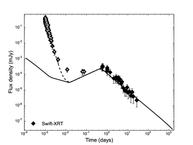
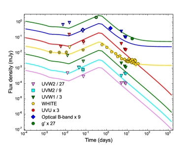
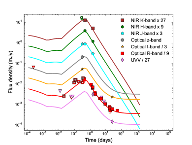
Figure 32.— X-ray (top left), UV (top right), optical (bottom left), and radio (bottom right) light curves of GRB 100418A in the wind scenario, with the full afterglow model (solid lines), including energy injection before 0.5 d.

Appendix D A Wind Model for GRB 100901A

We apply our MCMC analysis described in Section 6.2.2 to explore afterglow models with a wind-like circumburst environment for GRB 100901A. The parameters of the highest-likelihood model are $p\approx 2.02$, $\epsilon_{\rm e}\approx 0.33$, $\epsilon_{B}\approx 0.33$, $A_{*}\approx 1.7\times 10^{-2}$, $E_{\rm K,iso}\approx 3.8\times 10^{53}$, and $A_{\rm V}\lesssim 0.1$ mag. This model transitions from fast to slow cooling at $5.4\times 10^{-2}$ d. The spectral break frequencies at 1 d are located at $\nu_{\rm a}\approx 3.1\times 10^{8}$ Hz, $\nu_{\rm m}\approx 1.8\times 10^{12}$ Hz, and $\nu_{\rm c}\approx 1.7\times 10^{15}$ Hz, with $F_{\rm max}\approx 3.8$ mJy at 1 d, and a Compton $y$-parameter of 0.6. Like in the ISM model, $\nu_{\rm c}$is located between the optical and X-ray bands. Since the light curves in a wind environment decline faster than in the ISM case, the jet break in this model is later ($t_{\rm jet}\approx 3.5$ d) compared to the ISM model ($t_{\rm jet}\approx 1$ d). The jet opening angle is $\theta_{\rm jet}\approx 1.9$, resulting in a beaming-corrected kinetic energy of $2.0\times 10^{50}$ erg.

The summary statistics from our MCMC simulations are $p=2.027^{+0.005}_{-0.003}$, $E_{\rm K,iso}=(3.9\pm 0.5)\times 10^{53}$ erg, $A_{*}=1.9^{+0.3}_{-0.2}\times 10^{-2}$, $\epsilon_{\rm e}=0.32^{+0.01}_{-0.02}$, $\epsilon_{B}=0.27^{+0.04}_{-0.07}$, $A_{\rm V}\lesssim 0.1$ mag, $t_{\rm jet}=3.5\pm 0.2$ d, $\theta_{\rm jet}=1.9\pm 0.1\arcdeg$, $E_{\rm K}=(2.1\pm 0.2)\times 10^{50}\,$erg, and $E_{\gamma}=$. We plot histograms of the posterior density functions for these parameters in Figure 33 and present contours of the joint posterior density for the physical parameters $A_{*}$, $E_{\rm K,iso}$, $\epsilon_{\rm e}$, and $\epsilon_{B}$ in Figure 34.

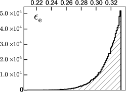
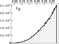
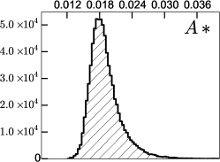
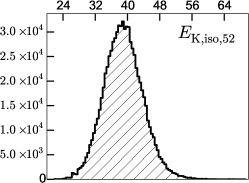
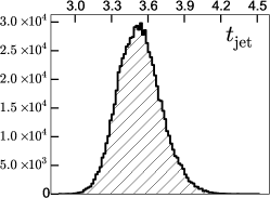
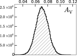
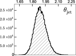
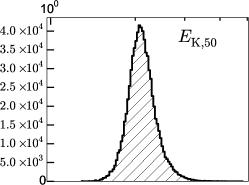
Figure 33.— Posterior probability density functions for the physical parameters for GRB 100901A in a wind environment from MCMC simulations. We have restricted $E_{\rm K,iso,52}<500$, $\epsilon_{\rm e}<\nicefrac{{1}}{{3}}$, and $\epsilon_{\rm B}<\nicefrac{{1}}{{3}}$.

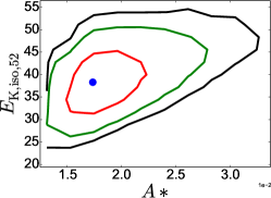
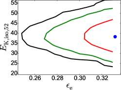
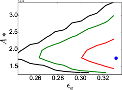
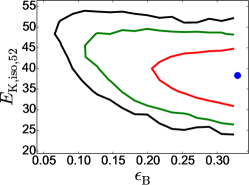
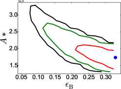
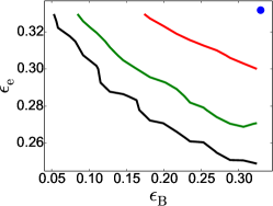
Figure 34.— 1$\sigma$ (red), 2$\sigma$ (green), and 3$\sigma$ (black) contours for correlations between the physical parameters, $E_{\rm K,iso}$, $n_{0}$, $\epsilon_{\rm e}$, and $\epsilon_{B}$ for GRB 100901A, in the wind model from Monte Carlo simulations. We have restricted $E_{\rm K,iso,52}<500$, $\epsilon_{\rm e}<\nicefrac{{1}}{{3}}$, and $\epsilon_{\rm B}<\nicefrac{{1}}{{3}}$. The highest-likelihood model is marked with a blue dot. See the on line version of this Figure for additional plots of correlations between these parameters and $p$, $A_{\rm V}$, $t_{\rm jet}$, $\theta_{\rm jet}$, and $E_{\rm K}$.

Like for GRBs 100418A and 120326A, it is challenging to fit both the X-ray and optical light curves before the bump together in the energy injection scenario under the wind model. Like for the wind model forGRB 120326A (Appendix B) and GRB 100418A (Appendix C), the optical light curves before the peak require a steeper injection rate than allowed by a distribution of Lorentz factors in the ejecta. In particular, our best energy injection model that matches the optical well but slightly under-predicts the X-ray data before 0.15 d (Figure 35), requires $E\propto t^{0.7}$ between $5\times 10^{-3}$ d and $0.12$ d, steepening to $E\propto t^{3.5}$ between $0.12$ d and $0.26$ d. In this model, the blastwave kinetic energy increases by a factor of 9 between $5\times 10^{-3}$ d and $0.12$ d, and another factor of $15$ between $0.12$ d and $0.26$ d, for an overall increase by a factor of $\approx 140$. Due to the discrepancy in the X-rays, the wind model may be considered a marginally viable model for GRB 100901A.

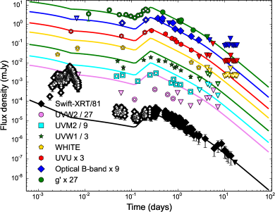
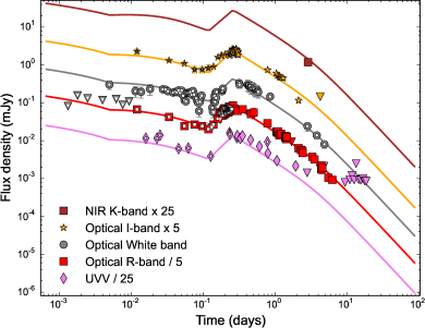
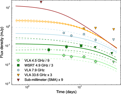
Figure 35.— X-ray and UV (top left), optical (top right), and radio (bottom left) light curves of GRB 100901A in the wind scenario, with the full afterglow model (solid lines), including energy injection before 0.26 d.

Appendix E A Wind Model for GRB 120404A

We apply the methods described in Section 6.3.2 to explore afterglow models with a wind-like circumburst environment for GRB 120404A. The parameters of our highest-likelihood model are $p\approx 2.03$, $\epsilon_{\rm e}\approx 0.33$, $\epsilon_{B}\approx 0.30$, $A_{*}\approx 1.9$, $E_{\rm K,iso}\approx 1.1\times 10^{53}$ erg, $t_{\rm jet}\approx 8.9\times 10^{-2}$ d, and $A_{\rm V}\approx 0.12$. This model also remains in spectrum 4 (Figure 17) for the duration of the observations, with the ordering $\nu_{\rm c}<\nu_{\rm a}<\nu_{\rm m}$. The spectral break frequencies are located at $\nu_{\rm ac}\approx 2.4\times 10^{10}$ Hz, $\nu_{\rm sa}\approx 7.9\times 10^{11}$ Hz, $\nu_{\rm m}\approx 4.0\times 10^{13}$ Hz, and $\nu_{\rm c}\approx 1.5\times 10^{10}$ Hz, at 0.1 d with $F_{\rm max}=F_{\nu,{\rm sa}}\approx 27$ mJy. The Compton $y$-parameter is 0.6.

The summary statistics (median and $68\%$ credible intervals) of the posterior density for these parameters are $p=2.04\pm 0.01$, $\epsilon_{\rm e}=0.28^{+0.03}_{-0.05}$, $\epsilon_{B}=0.18\pm 0.09$, $A_{*}=2.3^{+1.2}_{-0.7}$, $E_{\rm K,iso}=\left(1.2^{+0.3}_{-0.2}\right)\times 10^{53}$ erg, $t_{\rm jet}=(9.2\pm 0.6)\times 10^{-2}$ d, and $A_{\rm V}=0.13\pm 0.01$, corresponding to a jet opening angle of $\theta_{\rm jet}=3\arcdeg.0\pm 0\arcdeg.3$ and a beaming corrected kinetic energy of $E_{\rm K}=\left(1.6^{0.5}_{-0.3}\right)\times 10^{50}$ erg, the model match the data after the optical peak well (Figure 36). We present the correlation contours between the physical parameters in Figure 37 and the marginalized distributions for individual parameters in Figure 38.

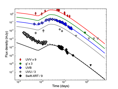
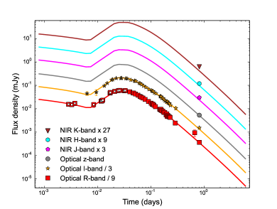
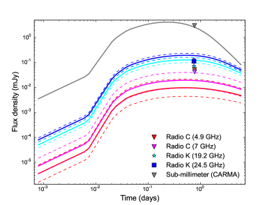
Figure 36.— Similar to Figure 20, but for a wind-like circumburst environment. The light curves before 0.04 d are based on the same energy injection model described in Section 6.3.3 as applied to the case of the wind medium. See Appendix E for a discussion.

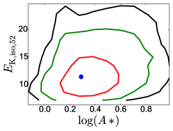
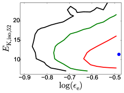
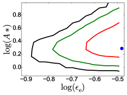
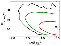
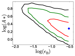
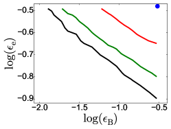
Figure 37.— 1$\sigma$ (red), 2$\sigma$ (green), and 3$\sigma$ (black) contours for correlations between the physical parameters, $E_{\rm K,iso}$, $n_{0}$, $\epsilon_{\rm e}$, and $\epsilon_{B}$ for GRB 120404A, in the wind model from Monte Carlo simulations. We have restricted $\epsilon_{\rm e}<\nicefrac{{1}}{{3}}$ and $\epsilon_{\rm B}<\nicefrac{{1}}{{3}}$. The highest-likelihood model is marked with a blue dot. See the on line version of this Figure for additional plots of correlations between these parameters and $p$, $t_{\rm jet}$, $\theta_{\rm jet}$, $E_{\rm K}$, and $A_{\rm V}$.

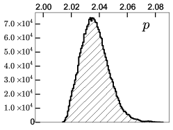
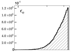
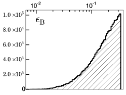
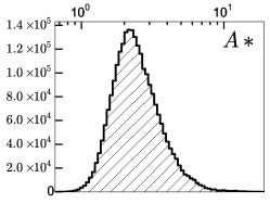
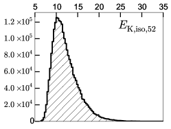
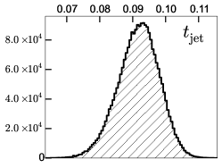
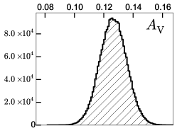
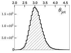
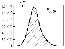
Figure 38.— Posterior probability density functions for the physical parameters for GRB 120404A in a wind environment from MCMC simulations. We have restricted $\epsilon_{\rm e}<\nicefrac{{1}}{{3}}$ and $\epsilon_{\rm B}<\nicefrac{{1}}{{3}}$.

The light curves before 0.04 d in Figure 36 are based on the same energy injection model as presented in Section 6.3.3. In this model, the energy increases by a factor of $\approx 27$ like in the the ISM case. However, the injection rate is not compatible with the maximum rate expected for a wind-like environment, similar to the other wind models (Appendices B, C, and D). We note that the optical and X-ray frequencies are located above both the cooling frequency and $\nu_{\rm m}$, with $\nu_{\rm c}<\nu_{\rm m}<\nu_{\rm opt}<\nu_{\rm X}$ in this case, and in this regime, the light curves are independent of the circumburst density profile. Thus the measurements do not allow us to distinguish between a wind or ISM-like environment in the case of GRB 120404A. Clear detections of a wind-like circumburst environment in conjunction with a steep energy injection rate in the future will enable us to furthur probe the massive ejecta model of energy injection in GRB afterglows, and thereby to further constrain the mechanism responsible for plateaus and re-brightening events in GRB afterglows.

References

- Amati et al. (2008) Amati, L., Guidorzi, C., Frontera, F., et al. 2008, MNRAS, 391, 577
- Andreev et al. (2010a) Andreev, M., Sergeev, A., & Pozanenko, A. 2010a, GRB Coordinates Network, 11166, 1
- Andreev et al. (2010b) —. 2010b, GRB Coordinates Network, 11168, 1
- Andreev et al. (2010c) —. 2010c, GRB Coordinates Network, 11191, 1
- Andreev et al. (2010d) —. 2010d, GRB Coordinates Network, 11201, 1
- Andreev et al. (2010e) Andreev, M., Sergeev, A., Pozanenko, A., et al. 2010e, GRB Coordinates Network, 11200, 1
- Antonelli et al. (2010) Antonelli, L. A., Maund, J. R., Palazzi, E., et al. 2010, GRB Coordinates Network, 10620, 1
- Barthelmy et al. (2005) Barthelmy, S. D., Barbier, L. M., Cummings, J. R., et al. 2005, Space Sci. Rev., 120, 143
- Barthelmy et al. (2012) Barthelmy, S. D., Sakamoto, T., Markwardt, C. B., et al. 2012, GRB Coordinates Network, 13120, 1
- Berger et al. (2000) Berger, E., Sari, R., Frail, D. A., et al. 2000, ApJ, 545, 56
- Berger et al. (2005) Berger, E., Price, P. A., Cenko, S. B., et al. 2005, Nature, 438, 988
- Bernardini et al. (2011) Bernardini, M. G., Margutti, R., Chincarini, G., Guidorzi, C., & Mao, J. 2011, A&A, 526, A27
- Blandford & McKee (1977) Blandford, R. D., & McKee, C. F. 1977, MNRAS, 180, 343
- Breeveld & Stratta (2012) Breeveld, A. A., & Stratta, G. 2012, GRB Coordinates Network, 13226, 1
- Burrows et al. (2005a) Burrows, D. N., Romano, P., Falcone, A., et al. 2005a, Science, 309, 1833
- Burrows et al. (2005b) Burrows, D. N., Hill, J. E., Nousek, J. A., et al. 2005b, Space Sci. Rev., 120, 165
- Cenko et al. (2006) Cenko, S. B., Fox, D. B., Moon, D.-S., et al. 2006, PASP, 118, 1396
- Cenko et al. (2010) Cenko, S. B., Frail, D. A., Harrison, F. A., et al. 2010, ApJ, 711, 641
- Cenko et al. (2011) —. 2011, ApJ, 732, 29
- Chandra & Frail (2010a) Chandra, P., & Frail, D. A. 2010a, GRB Coordinates Network, 11257, 1
- Chandra & Frail (2010b) —. 2010b, GRB Coordinates Network, 10650, 1
- Chandra et al. (2008) Chandra, P., Cenko, S. B., Frail, D. A., et al. 2008, ApJ, 683, 924
- Chevalier & Li (2000) Chevalier, R. A., & Li, Z.-Y. 2000, ApJ, 536, 195
- Chiang & Dermer (1999) Chiang, J., & Dermer, C. D. 1999, ApJ, 512, 699
- Chincarini et al. (2007) Chincarini, G., Moretti, A., Romano, P., et al. 2007, ApJ, 671, 1903
- Chincarini et al. (2010) Chincarini, G., Mao, J., Margutti, R., et al. 2010, MNRAS, 406, 2113
- Chornock et al. (2010) Chornock, R., Berger, E., Fox, D., et al. 2010, GRB Coordinates Network, 11164, 1
- Collazzi (2012) Collazzi, A. C. 2012, GRB Coordinates Network, 13145, 1
- Covino et al. (2008) Covino, S., D’Avanzo, P., Klotz, A., et al. 2008, MNRAS, 388, 347
- Cucchiara & Tanvir (2012) Cucchiara, A., & Tanvir, N. R. 2012, GRB Coordinates Network, 13217, 1
- Dai & Lu (1998) Dai, Z. G., & Lu, T. 1998, A&A, 333, L87
- Dall’Osso et al. (2011) Dall’Osso, S., Stratta, G., Guetta, D., et al. 2011, A&A, 526, A121
- De Cia et al. (2010) De Cia, A., Vreeswijk, P. M., & Jakobsson, P. 2010, GRB Coordinates Network, 11170, 1
- de Ugarte Postigo et al. (2007) de Ugarte Postigo, A., Fatkhullin, T. A., Jóhannesson, G., et al. 2007, A&A, 462, L57
- Dermer et al. (2000a) Dermer, C. D., Böttcher, M., & Chiang, J. 2000a, ApJ, 537, 255
- Dermer et al. (2000b) Dermer, C. D., Chiang, J., & Mitman, K. E. 2000b, ApJ, 537, 785
- Duffell & MacFadyen (2014) Duffell, P. C., & MacFadyen, A. I. 2014, ArXiv e-prints, arXiv:1407.8250
- Eichler & Granot (2006) Eichler, D., & Granot, J. 2006, ApJ, 641, L5
- Elenin et al. (2010a) Elenin, L., Molotov, I., & Pozanenko, A. 2010a, GRB Coordinates Network, 11184, 1
- Elenin et al. (2010b) —. 2010b, GRB Coordinates Network, 11234, 1
- Evans et al. (2007) Evans, P. A., Beardmore, A. P., Page, K. L., et al. 2007, A&A, 469, 379
- Evans et al. (2009) —. 2009, MNRAS, 397, 1177
- Falcone et al. (2006) Falcone, A. D., Burrows, D. N., Lazzati, D., et al. 2006, ApJ, 641, 1010
- Fan & Piran (2006) Fan, Y., & Piran, T. 2006, MNRAS, 369, 197
- Fan & Wei (2005) Fan, Y. Z., & Wei, D. M. 2005, MNRAS, 364, L42
- Filgas et al. (2010) Filgas, R., Klose, S., & Greiner, J. 2010, GRB Coordinates Network, 10617, 1
- Foreman-Mackey et al. (2013) Foreman-Mackey, D., Hogg, D. W., Lang, D., & Goodman, J. 2013, PASP, 125, 306
- Frail et al. (2000) Frail, D. A., Waxman, E., & Kulkarni, S. R. 2000, ApJ, 537, 191
- Frail et al. (2003) Frail, D. A., Yost, S. A., Berger, E., et al. 2003, ApJ, 590, 992
- Friedman & Bloom (2005) Friedman, A. S., & Bloom, J. S. 2005, ApJ, 627, 1
- Gehrels et al. (2004) Gehrels, N., Chincarini, G., Giommi, P., et al. 2004, ApJ, 611, 1005
- Ghirlanda et al. (2007) Ghirlanda, G., Nava, L., Ghisellini, G., & Firmani, C. 2007, A&A, 466, 127
- Gorbovskoy et al. (2010) Gorbovskoy, E., Lipunov, V., Kornilov, V., et al. 2010, GRB Coordinates Network, 11178, 1
- Gorbovskoy et al. (2012) —. 2012, GRB Coordinates Network, 13230, 1
- Gorbovskoy et al. (2012) Gorbovskoy, E. S., Lipunova, G. V., Lipunov, V. M., et al. 2012, MNRAS, 421, 1874
- Granot et al. (2006) Granot, J., Königl, A., & Piran, T. 2006, MNRAS, 370, 1946
- Granot & Kumar (2006) Granot, J., & Kumar, P. 2006, MNRAS, 366, L13
- Granot et al. (2001) Granot, J., Miller, M., Piran, T., Suen, W., & Hughes, P. 2001, in Gamma-Ray Bursts in the Afterglow Era, ed. E. Costa, F. Frontera, & J. Hjorth, ESO ASTROPHYSICS SYMPOSIA (http://arxiv.org/pdf/astro-ph/0103038.pdf: Springer Berlin Heidelberg), 312–314
- Granot et al. (2002) Granot, J., Panaitescu, A., Kumar, P., & Woosley, S. E. 2002, ApJ, 570, L61
- Granot & Sari (2002) Granot, J., & Sari, R. 2002, ApJ, 568, 820
- Greisen (2003) Greisen, E. W. 2003, Information Handling in Astronomy - Historical Vistas, 285, 109
- Guidorzi et al. (2015) Guidorzi, C., Dichiara, S., Frontera, F., et al. 2015, ApJ, 801, 57
- Guidorzi et al. (2012) Guidorzi, C., Melandri, A., & Japelj, J. 2012, GRB Coordinates Network, 13209, 1
- Guidorzi et al. (2007) Guidorzi, C., Vergani, S. D., Sazonov, S., et al. 2007, A&A, 474, 793
- Guidorzi et al. (2013) Guidorzi, C., Mundell, C. G., Harrison, R., et al. 2013, MNRAS, arXiv:1311.4340
- Harrison et al. (2001) Harrison, F. A., Yost, S. A., Sari, R., et al. 2001, ApJ, 559, 123
- Hascoet et al. (2015) Hascoet, R., Beloborodov, A. M., Daigne, F., & Mochkovitch, R. 2015, ArXiv e-prints, arXiv:1503.08333
- Hascoët et al. (2012) Hascoët, R., Daigne, F., & Mochkovitch, R. 2012, A&A, 541, A88
- Hentunen et al. (2010) Hentunen, V.-P., Nissinen, M., & Salmi, T. 2010, GRB Coordinates Network, 11173, 1
- Hentunen et al. (2012) —. 2012, GRB Coordinates Network, 13119, 1
- Ho et al. (2004) Ho, P. T. P., Moran, J. M., & Lo, K. Y. 2004, ApJ, 616, L1
- Hou et al. (2014) Hou, S. J., Geng, J. J., Wang, K., et al. 2014, ApJ, 785, 113
- Im et al. (2010) Im, M., Choi, C., Jun, H., et al. 2010, GRB Coordinates Network, 11208, 1
- Immler et al. (2010) Immler, S., Barthelmy, S. D., Baumgartner, W. H., et al. 2010, GRB Coordinates Network, 11159, 1
- Jang et al. (2012) Jang, M., Im, M., & Urata, Y. 2012, GRB Coordinates Network, 13139, 1
- Jester et al. (2005) Jester, S., Schneider, D. P., Richards, G. T., et al. 2005, AJ, 130, 873
- Jin et al. (2007) Jin, Z. P., Yan, T., Fan, Y. Z., & Wei, D. M. 2007, ApJ, 656, L57
- Kalberla et al. (2005) Kalberla, P. M. W., Burton, W. B., Hartmann, D., et al. 2005, A&A, 440, 775
- Kann et al. (2010a) Kann, D. A., Laux, U., & Stecklum, B. 2010a, GRB Coordinates Network, 11236, 1
- Kann et al. (2010b) Kann, D. A., Ludwig, F., & Stecklum, B. 2010b, GRB Coordinates Network, 11246, 1
- Klotz et al. (2012) Klotz, A., Gendre, B., Boer, M., & Atteia, J. L. 2012, GRB Coordinates Network, 13108, 1
- Kobayashi (2000) Kobayashi, S. 2000, ApJ, 545, 807
- Kobayashi & Sari (2000) Kobayashi, S., & Sari, R. 2000, ApJ, 542, 819
- Kobayashi & Zhang (2003) Kobayashi, S., & Zhang, B. 2003, ApJ, 597, 455
- Kong et al. (2010) Kong, S. W., Wong, A. Y. L., Huang, Y. F., & Cheng, K. S. 2010, MNRAS, 402, 409
- Kopac et al. (2010) Kopac, D., Dintinjana, B., & Gomboc, A. 2010, GRB Coordinates Network, 11177, 1
- Kuin et al. (2012) Kuin, N. P. M., Holland, S., & Siegel, M. H. 2012, GRB Coordinates Network, 13114, 1
- Kumar & Piran (2000) Kumar, P., & Piran, T. 2000, ApJ, 532, 286
- Kuroda et al. (2010a) Kuroda, D., Hanayama, H., Miyaji, T., et al. 2010a, GRB Coordinates Network, 11258, 1
- Kuroda et al. (2010b) —. 2010b, GRB Coordinates Network, 11205, 1
- Kuroda et al. (2010c) Kuroda, D., Yanagisawa, K., Shimizu, Y., et al. 2010c, GRB Coordinates Network, 11172, 1
- Kuroda et al. (2010d) —. 2010d, GRB Coordinates Network, 11189, 1
- Lacluyze et al. (2012) Lacluyze, A., Haislip, J., Ivarsen, K., et al. 2012, GRB Coordinates Network, 13109, 1
- Landolt (2009) Landolt, A. U. 2009, AJ, 137, 4186
- Laskar et al. (2013) Laskar, T., Berger, E., Zauderer, B. A., et al. 2013, ApJ, 776, 119
- Laskar et al. (2014) Laskar, T., Berger, E., Tanvir, N., et al. 2014, ApJ, 781, 1
- Lazzati & Perna (2007) Lazzati, D., & Perna, R. 2007, MNRAS, 375, L46
- Lazzati et al. (2002) Lazzati, D., Rossi, E., Covino, S., Ghisellini, G., & Malesani, D. 2002, A&A, 396, L5
- Li et al. (2012) Li, L., Liang, E.-W., Tang, Q.-W., et al. 2012, ApJ, 758, 27
- Liang et al. (2007) Liang, E.-W., Zhang, B.-B., & Zhang, B. 2007, ApJ, 670, 565
- Liang et al. (2006) Liang, E. W., Zhang, B., O’Brien, P. T., et al. 2006, ApJ, 646, 351
- Lipkin et al. (2004) Lipkin, Y. M., Ofek, E. O., Gal-Yam, A., et al. 2004, ApJ, 606, 381
- Liu et al. (2008) Liu, X. W., Wu, X. F., & Lu, T. 2008, A&A, 487, 503
- Malesani & Palazzi (2010) Malesani, D., & Palazzi, E. 2010, GRB Coordinates Network, 10631, 1
- Malesani et al. (2007) Malesani, D., Covino, S., D’Avanzo, P., et al. 2007, A&A, 473, 77
- Mangano et al. (2007) Mangano, V., Holland, S. T., Malesani, D., et al. 2007, A&A, 470, 105
- Margutti et al. (2011a) Margutti, R., Bernardini, G., Barniol Duran, R., et al. 2011a, MNRAS, 410, 1064
- Margutti et al. (2010a) Margutti, R., Guidorzi, C., Chincarini, G., et al. 2010a, MNRAS, 406, 2149
- Margutti et al. (2010b) Margutti, R., Genet, F., Granot, J., et al. 2010b, MNRAS, 402, 46
- Margutti et al. (2011b) Margutti, R., Chincarini, G., Granot, J., et al. 2011b, MNRAS, 417, 2144
- Margutti et al. (2013) Margutti, R., Zaninoni, E., Bernardini, M. G., et al. 2013, MNRAS, 428, 729
- Marshall et al. (2010) Marshall, F. E., Beardmore, A. P., Gelbord, J. M., et al. 2010, GRB Coordinates Network, 10612, 1
- Marshall et al. (2011) Marshall, F. E., Antonelli, L. A., Burrows, D. N., et al. 2011, ApJ, 727, 132
- Melandri et al. (2014) Melandri, A., Virgili, F. J., Guidorzi, C., et al. 2014, A&A, 572, A55
- Moin et al. (2010) Moin, A., Tingay, S., Phillips, C., et al. 2010, GRB Coordinates Network, 10832, 1
- Moin et al. (2013) Moin, A., Chandra, P., Miller-Jones, J. C. A., et al. 2013, ApJ, 779, 105
- Monfardini et al. (2006) Monfardini, A., Kobayashi, S., Guidorzi, C., et al. 2006, ApJ, 648, 1125
- Moody et al. (2010) Moody, J. W., Laney, D., Pearson, R., & Pace, C. 2010, GRB Coordinates Network, 10665, 1
- Morgan (2012) Morgan, A. N. 2012, GRB Coordinates Network, 13143, 1
- Nakar & Granot (2007) Nakar, E., & Granot, J. 2007, MNRAS, 380, 1744
- Nousek et al. (2006) Nousek, J. A., Kouveliotou, C., Grupe, D., et al. 2006, ApJ, 642, 389
- O’Brien et al. (2006) O’Brien, P. T., Willingale, R., Osborne, J., et al. 2006, ApJ, 647, 1213
- Pagani et al. (2006) Pagani, C., Morris, D. C., Kobayashi, S., et al. 2006, ApJ, 645, 1315
- Page & Immler (2010) Page, K. L., & Immler, S. 2010, GRB Coordinates Network, 11171, 1
- Panaitescu & Kumar (2000) Panaitescu, A., & Kumar, P. 2000, ApJ, 543, 66
- Panaitescu & Kumar (2001) —. 2001, ApJ, 554, 667
- Panaitescu & Kumar (2002) —. 2002, ApJ, 571, 779
- Panaitescu & Mészáros (1998) Panaitescu, A., & Mészáros, P. 1998, ApJ, 501, 772
- Panaitescu et al. (2006) Panaitescu, A., Mészáros, P., Gehrels, N., Burrows, D., & Nousek, J. 2006, MNRAS, 366, 1357
- Panaitescu et al. (2013) Panaitescu, A., Vestrand, W. T., & Woźniak, P. 2013, MNRAS, 433, 759
- Pandey & Zheng (2010) Pandey, S. B., & Zheng, W. 2010, GRB Coordinates Network, 11179, 1
- Pei (1992) Pei, Y. C. 1992, ApJ, 395, 130
- Perley et al. (2012) Perley, D. A., Alatalo, K., & Horesh, A. 2012, GRB Coordinates Network, 13175, 1
- Perna et al. (2006) Perna, R., Armitage, P. J., & Zhang, B. 2006, ApJ, 636, L29
- Phinney (1989) Phinney, E. S. 1989, in IAU Symposium, Vol. 136, The Center of the Galaxy, ed. M. Morris, 543
- Piro et al. (1998) Piro, L., Amati, L., Antonelli, L. A., et al. 1998, A&A, 331, L41
- Pritchard & Immler (2010) Pritchard, T. A., & Immler, S. 2010, GRB Coordinates Network, 11176, 1
- Proga & Zhang (2006) Proga, D., & Zhang, B. 2006, MNRAS, 370, L61
- Rees & Meszaros (1998) Rees, M. J., & Meszaros, P. 1998, ApJ, 496, L1
- Rhoads (1999) Rhoads, J. E. 1999, ApJ, 525, 737
- Romano et al. (2006) Romano, P., Moretti, A., Banat, P. L., et al. 2006, A&A, 450, 59
- Roming et al. (2005) Roming, P. W. A., Kennedy, T. E., Mason, K. O., et al. 2005, Space Sci. Rev., 120, 95
- Rujopakarn & Flewelling (2012) Rujopakarn, W., & Flewelling, H. 2012, GRB Coordinates Network, 13106, 1
- Rumyantsev et al. (2010) Rumyantsev, V., Shakhovkoy, D., & Pozanenko, A. 2010, GRB Coordinates Network, 11255, 1
- Sahu et al. (2012) Sahu, D. K., Anupama, G. C., & Pandey, S. B. 2012, GRB Coordinates Network, 13185, 1
- Sahu et al. (2010a) Sahu, D. K., Arora, S., Singh, N. S., & Kartha, S. S. 2010a, GRB Coordinates Network, 11197, 1
- Sahu et al. (2010b) Sahu, D. K., Bhatt, B. C., & Arora, S. 2010b, GRB Coordinates Network, 11175, 1
- Salvaterra et al. (2009) Salvaterra, R., Della Valle, M., Campana, S., et al. 2009, Nature, 461, 1258
- Sari & Esin (2001) Sari, R., & Esin, A. A. 2001, ApJ, 548, 787
- Sari & Mészáros (2000) Sari, R., & Mészáros, P. 2000, ApJ, 535, L33
- Sari et al. (1996) Sari, R., Narayan, R., & Piran, T. 1996, ApJ, 473, 204
- Sari et al. (1999) Sari, R., Piran, T., & Halpern, J. P. 1999, ApJ, 519, L17
- Sari et al. (1998) Sari, R., Piran, T., & Narayan, R. 1998, ApJ, 497, L17+
- Sault et al. (1995) Sault, R. J., Teuben, P. J., & Wright, M. C. H. 1995, in Astronomical Society of the Pacific Conference Series, Vol. 77, Astronomical Data Analysis Software and Systems IV, ed. R. A. Shaw, H. E. Payne, & J. J. E. Hayes, 433
- Schaefer et al. (2003) Schaefer, B. E., Gerardy, C. L., Höflich, P., et al. 2003, ApJ, 588, 387
- Shao & Dai (2007) Shao, L., & Dai, Z. G. 2007, ApJ, 660, 1319
- Shen et al. (2008) Shen, R.-F., Barniol Duran, R., & Kumar, P. 2008, MNRAS, 384, 1129
- Siegel & Marshall (2010) Siegel, M. H., & Marshall, F. 2010, GRB Coordinates Network, 10625, 1
- Siegel et al. (2012) Siegel, M. H., Barthelmy, S. D., Burrows, D. N., et al. 2012, GRB Coordinates Network, 13105, 1
- Sposetti & Immler (2010) Sposetti, S., & Immler, S. 2010, GRB Coordinates Network, 11213, 1
- Stratta et al. (2012) Stratta, G., Barthelmy, S. D., Baumgartner, W. H., et al. 2012, GRB Coordinates Network, 13208, 1
- Sudilovsky et al. (2012) Sudilovsky, V., Nicuesa Guelbenzu, A., & Greiner, J. 2012, GRB Coordinates Network, 13129, 1
- Tagliaferri et al. (2005) Tagliaferri, G., Goad, M., Chincarini, G., et al. 2005, Nature, 436, 985
- Tello et al. (2012) Tello, J. C., Sanchez-Ramirez, R., Gorosabel, J., et al. 2012, GRB Coordinates Network, 13118, 1
- Toma et al. (2006) Toma, K., Ioka, K., Yamazaki, R., & Nakamura, T. 2006, ApJ, 640, L139
- Totani (1998) Totani, T. 1998, ApJ, 502, L13
- Uhm & Zhang (2014) Uhm, Z. L., & Zhang, B. 2014, ApJ, 789, 39
- Uhm et al. (2012) Uhm, Z. L., Zhang, B., Hascoët, R., et al. 2012, ApJ, 761, 147
- Ukwatta et al. (2010) Ukwatta, T. N., Sakamoto, T., Gehrels, N., & Dhuga, K. S. 2010, GRB Coordinates Network, 11198, 1
- Ukwatta et al. (2012) Ukwatta, T. N., Barthelmy, S. D., Baumgartner, W. H., et al. 2012, GRB Coordinates Network, 13220, 1
- Updike et al. (2010a) Updike, A. C., Hartmann, D. H., & de Pree, C. 2010a, GRB Coordinates Network, 10637, 1
- Updike et al. (2010b) Updike, A. C., Hartmann, D. H., Keel, W., & Darnell, E. 2010b, GRB Coordinates Network, 11174, 1
- Updike et al. (2010c) Updike, A. C., Hartmann, D. H., & Murphy, B. 2010c, GRB Coordinates Network, 10619, 1
- Urata et al. (2014) Urata, Y., Huang, K., Takahashi, S., et al. 2014, ApJ, 789, 146
- van der Horst et al. (2010a) van der Horst, A. J., Kamble, A. P., Wijers, R. A. M. J., et al. 2010a, GRB Coordinates Network, 10647, 1
- van der Horst et al. (2010b) van der Horst, A. J., Wiersema, K., Kamble, A. P., et al. 2010b, GRB Coordinates Network, 11221, 1
- Volnova et al. (2010) Volnova, A., Pozanenko, A., Ibrahimov, M., Hafizov, B., & Satovski, B. 2010, GRB Coordinates Network, 11266, 1
- Volnova et al. (2012) Volnova, A., Sinyakov, E., Varda, D., & Molotov, I. 2012, GRB Coordinates Network, 13198, 1
- Wang et al. (2006) Wang, X.-Y., Li, Z., & Mészáros, P. 2006, ApJ, 641, L89
- Wei & Lu (1998) Wei, D. M., & Lu, T. 1998, ApJ, 505, 252
- Willingale et al. (2010) Willingale, R., Genet, F., Granot, J., & O’Brien, P. T. 2010, MNRAS, 403, 1296
- Wilson et al. (2003) Wilson, J. C., Eikenberry, S. S., Henderson, C. P., et al. 2003, in Society of Photo-Optical Instrumentation Engineers (SPIE) Conference Series, Vol. 4841, Society of Photo-Optical Instrumentation Engineers (SPIE) Conference Series, ed. M. Iye & A. F. M. Moorwood, 451–458
- Xin et al. (2012a) Xin, L. P., Wei, J. Y., Qiu, Y. L., et al. 2012a, GRB Coordinates Network, 13150, 1
- Xin et al. (2012b) —. 2012b, GRB Coordinates Network, 13221, 1
- Xin et al. (2012) Xin, L. P., Pozanenko, A., Kann, D. A., et al. 2012, MNRAS, 422, 2044
- Yoshida et al. (2010) Yoshida, M., Sasada, M., Komatsu, T., & Kawabata, K. S. 2010, GRB Coordinates Network, 11190, 1
- Yost et al. (2003) Yost, S. A., Harrison, F. A., Sari, R., & Frail, D. A. 2003, ApJ, 597, 459
- Yost et al. (2002) Yost, S. A., Frail, D. A., Harrison, F. A., et al. 2002, ApJ, 577, 155
- Yu & Dai (2007) Yu, Y. W., & Dai, Z. G. 2007, A&A, 470, 119
- Zauderer et al. (2012) Zauderer, A., Laskar, T., & Berger, E. 2012, GRB Coordinates Network, 13231, 1
- Zhang et al. (2006) Zhang, B., Fan, Y. Z., Dyks, J., et al. 2006, ApJ, 642, 354
- Zhang & Mészáros (2001) Zhang, B., & Mészáros, P. 2001, ApJ, 552, L35
- Zhang & Mészáros (2002) —. 2002, ApJ, 566, 712
- Zhang et al. (2007) Zhang, B., Liang, E., Page, K. L., et al. 2007, ApJ, 655, 989
- Zhao et al. (2012) Zhao, X.-H., Mao, J., Xu, D., & Bai, J.-M. 2012, GRB Coordinates Network, 13122, 1
- Zou et al. (2005) Zou, Y. C., Wu, X. F., & Dai, Z. G. 2005, MNRAS, 363, 93