Probabilistic Clustering of
Time-Evolving Distance Data

Abstract

We present a novel probabilistic clustering model for objects that are represented via pairwise distances and observed at different time points. The proposed method utilizes the information given by adjacent time points to find the underlying cluster structure and obtain a smooth cluster evolution. This approach allows the number of objects and clusters to differ at every time point, and no identification on the identities of the objects is needed. Further, the model does not require the number of clusters being specified in advance – they are instead determined automatically using a Dirichlet process prior. We validate our model on synthetic data showing that the proposed method is more accurate than state-of-the-art clustering methods. Finally, we use our dynamic clustering model to analyze and illustrate the evolution of brain cancer patients over time.

1 Introduction

A major challenge in data analysis is to find simple representations of the data that best reveal the underlying structure of the investigated phenomenon [15]. Clustering is a powerful tool to detect such structure in empirical data, thus making it accessible to practitioners [14]. The problem of clustering has a very long history in the data mining and machine learning communities, and numerous clustering algorithms and applications have been studied in many different scientific disciplines over the past 50 years [13]. Applications of clustering include a large variety of problem domains as, for example, clustering text, social networks, images, or biomedical data [4, 10, 21, 28]. Traditional clustering methods such as $k$-means or Gaussian mixture models [12], rely on geometric representation of the data. Nowadays, however, increasingly often there is no access to an underlying vectorial representation of the data since only pairwise similarities or distances are measured. An example application domain where such a setting frequently occurs is biomedical data analysis, where more often than not only pairwise distance data is available, e.g., when DNA or protein sequences are represented as pairwise distances or string alignments [9, 16, 23, 25, 26].
Although many clustering methods exist that work on distance data, including single linkage clustering, complete linkage clustering, and Ward’s clustering [14], these methods are static methods that are innocuous with respect to a potentially underlying time structure. However, when data is obtained at different points in time, dynamic models are needed that take a time component into account. For example in cancer research, genes are frequently measured at different time points, in order to examine the efficiency of a medication over time. In Network Security, HTTP connections are recorded at various timestamps, since network behaviors can quickly change over time; in Computer Vision, video streams contain time-indexed sequence of images. To deal with such scenarios, dynamic models that take the evolving nature of data into account are needed. Such a requirement has been addressed with evolutionary or dynamic clustering models for vectorial data (as for instance in [2], [7], [29], or [33]), which obtain a smooth clustering over multiple time points. However, to the best of our knowledge, no time-evolving clustering models exist that work on distance data directly, and clustering of time-evolving distance data is still an unsolved problem.
In this work we will bridge this gap and present a novel Bayesian time-evolving clustering model based on distance data directly that is specially tailored to temporal data and does not require direct access to an underlying vector space. Our model will be able to detect cluster popularity over time, based on the rich gets richer phenomenon. We will be able to make predictions about how popular a cluster will be at time $t+1$ if we already knew that it was a rich cluster at time point $t$. The assumption that rich clusters get richer seems plausible in many domains, for instance, a hot news topic is likely to stay hot for a given time period. Our model is also able to cope with variability of data size: the number of data points may vary between time points, for instance, data items may arrive or leave. Also, the number of clusters may vary over time and the model is able to adjust its capacity accordingly, and automatically. The aim is to find the underlying structure at every time point and to obtain a smooth cluster evolution which results in an easy interpretable model. Thereby the information shared across neighboring time points is related to the size of the clusters, the time-varying property of the clusters is assumed to be Markovian, and Markov Chain Monte Carlo (MCMC) sampling is used for inference.
The presented method is also applicable for the less general case of pairwise similarity data, by using a slightly altered likelihood. Since Mercer kernels can encode similarities between many different kinds of objects (for instance kernels on graphs, images, structures or strings) the method proposed here can in particularly cover the entire scope of applications of kernel-based learning, be it string alignment kernels over DNA or protein sequences [16, 23, 26] or diffusion kernels on graphs [30].
We validate our approach by comparing it to baseline methods on simulated data where our new model significantly outperforms state-of-the-art clustering approaches. We apply our novel model to a highly topical and challenging real world data set of brain cancer patients from Memorial Sloan Kettering Cancer Center (MSKCC). This data consists of clinical notes as part of electronic health records (EHR) of brain cancer patients over 3 consecutive years. We model brain cancer patients over time where patients are grouped together based on the similarity of sentences in the clinical notes (see Section 4.2).

2 Background

In this section we recap important background knowledge which is essential for the remainder of this paper.

Partition Process:

Let $\mathbb{B}_{n}$ denote a set of partitions of $[n]$, and $[n]:=\{1,\dots,n\}$ denote an index set. A partition $B\in\mathbb{B}_{n}$ is an equivalence relation $B:[n]\times[n]\to\{0,1\}$ with $B(i,j)=1$ if $y(i)=y(j)$ and $B(i,j)=0$ otherwise. $y$ denotes a function that maps $[n]$ to some label set $\mathbb{L}$. Alternatively, $B$ may be represented as a set of disjoint non-empty subsets called “blocks”. A partition process is a series of distributions $P_{n}$ on the set $\mathbb{B}_{n}$ in which $P_{n}$ is the marginal distribution of $P_{n+1}$. This means, that for each partition $B\in\mathbb{B}_{n+1}$, there exists a corresponding partition $B^{*}\in\mathbb{B}_{n}$ which is obtained by deleting the last row and column from the matrix $B$. The properties of partition processes are in detail discussed in [19]. Such a process is called exchangeable if each $P_{n}$ is invariant under permutations of object indices, see [22] for more details. An example for the partition lattice for $\mathbb{B}_{3}$ is shown in Fig. 1.

Figure 1: Partition lattice for $\mathbb{B}_{3}$.

Gauss-Dirichlet Cluster Process:

The Gauss-Dirichlet cluster process consists of an infinite sequence of points in $\mathbb{R}^{d}$, together with a random partition of integers into $k$ blocks. A sequence of length $n$ can be sampled as follows [17, 19]: fix the number of mixture modes $k$, generate mixing proportions $\pi=(\pi_{1},\dots,\pi_{k})$ from a symmetric Dirichlet distribution Dir$(\xi/k,\dots,\xi/k)$, generate a label sequence $\{y(1),\dots,y(n)\}$ from a multinomial distribution and forget the labels introducing the random partition $B$ of $[n]$ induced by $y$. Integrating out $\pi$, one arrives at a Dirichlet-Multinomial prior over partitions

$$P_{n}(B|\xi,k)=\frac{k!}{(k-k_{B})!}\frac{\Gamma(\xi)\prod_{b\in B}\Gamma(n_{b}+\xi/k)}{\Gamma(n+\xi)[\Gamma(\xi/k)]^{k_{B}}},$$ (1)

where $k_{B}\leq k$ denotes the number of blocks present in the partition $B$ and $n_{b}$ is the size of block $b$. The limit as $k\to\infty$ is well defined and known as the Ewens process (a.k.a. Chinese Restaurant process (CRP)), see for instance [11, 20, 6]. Given such a partition $B$, a sequence of $n$-dimensional observations $\boldsymbol{x}_{i}\in\mathbb{R}^{n},\;i=1,\dots,d$, is arranged as columns of the $(n\times d)$ matrix ${X}$, and this $X$ is generated from a zero-mean Gaussian distribution with covariance matrix

$$\widetilde{\Sigma}_{B}=I_{n}\otimes\Sigma_{0}+B\otimes\Sigma_{1},\quad\text{ with }\quad\text{cov}({X}_{ir},{X}_{js}|B)=\delta_{ij}{\Sigma_{0}}_{rs}+B_{ij}{\Sigma_{1}}_{rs}.$$ (2)

$\Sigma_{0}$ denotes the $(d\times d)$ within-class covariance matrix and $\Sigma_{1}$ the $(d\times d)$ between-class matrix, respectively, and $\delta_{ij}$ denotes the Kronecker symbol. Since the partition process is invariant under permutations, we can always think of $B$ being block-diagonal. For spherical covariance matrices (i.e. scaled identity matrices), $\Sigma_{0}=\alpha I_{d},\Sigma_{1}=\beta I_{d}$, the covariance structure reduces to $\textstyle\widetilde{\Sigma}_{B}=I_{n}\otimes\alpha I_{d}+B\otimes\beta I_{d}\\ =(\alpha I_{n}+\beta B)\otimes I_{d}=:\Sigma_{B}\otimes I_{d},\text{ with }\text{cov}({X}_{ir},{X}_{js}|B)=(\alpha\delta_{ij}+\beta B_{ij})\delta_{rs}.$ Thus, the columns of ${X}$ contain independent $n$-dimensional vectors $\boldsymbol{x}_{i}\in\mathbb{R}^{n}$ distributed according to a normal distribution with covariance matrix

$$\Sigma_{B}=\alpha I_{n}+\beta B.$$ (3)

Further, the distribution factorizes over the blocks $b\in B$. Introducing the symbol ${i_{b}}:=\{i:i\in b\}$ defining an index-vector of all objects assigned to block $b$, the joint distribution reads

$$\textstyle p(X,B|\alpha,\beta,\xi,k)=P_{n}(B|\xi,k)\textstyle\cdot\left[\prod_{b\in B}\prod_{j=1}^{d}\mathcal{N}(X_{{i_{b}}j}|\alpha I_{n_{b}}+\beta\boldsymbol{1}_{n_{b}}\boldsymbol{1}^{t}_{n_{b}})\right],$$ (4)

where $n_{b}$ is the size of block $b$ and $\boldsymbol{1}_{n_{b}}$ a $n_{b}$-vector of ones. In the viewpoint of clustering, $n$ denote the number of objects we want to partition, and $d$ the dimension of each object.

Wishart-Dirichlet Cluster Process:

Assume that the random matrix ${X}_{n\times d}$ follows the zero-mean Gaussian distribution specified in (2), with $\Sigma_{0}=\alpha I_{d}$ and $\Sigma_{1}=\beta I_{d}$. Then, conditioned on the partition $B$, the inner product matrix ${K}={X}{X}^{t}/d$ follows a (possibly singular) Wishart distribution in $d$ degrees of freedom, ${K}\sim\mathcal{W}_{d}(\Sigma_{B})$, as was shown in [27]. If we directly observe the dot products $K$, it suffices to consider the conditional probability of partitions $P_{n}(B|K)$:

$$\textstyle\begin{split}&\textstyle P_{n}(B|K,\alpha,\beta,\xi,k)\propto\mathcal{W}_{d}(K|\Sigma_{B})\cdot P_{n}(B|\xi,k)\\ &\textstyle\propto\left|{\Sigma_{B}}\right|^{-\frac{d}{2}}\exp\left(-\frac{d}{2}{\rm tr}(\Sigma_{B}^{-1}K)\right)\cdot P_{n}(B|\xi,k)\end{split}$$ (5)

Information Loss:

Note that we assumed that there exists a matrix $X$ with ${K}={X}{X}^{t}/d$ such that the columns of $X$ are independent copies drawn from a zero-mean Gaussian in $\mathbb{R}^{n}$: $\boldsymbol{x}\sim N(\boldsymbol{\mu}=\boldsymbol{0}_{n},\Sigma=\Sigma_{B})$. This assumption is crucial, since general mean vectors correspond to a non-central Wishart model [3], which can be calculated analytically only in special cases, and even these cases have a very complicated form which imposes severe problems in deriving efficient inference algorithms.
By moving from vectors $X$ to pairwise similarities $K$ and from similarities to pairwise distances $D$, there is a lack of information about geometric transformations: assume we only observe $K$ without access to the vectorial representations $X_{n\times d}$. Then we have lost the information about orthogonal transformations $X\leftarrow XO$ with $OO^{t}=I_{d}$, i.e. about rotations and reflections of the rows in $X$. If we only observe $D$, we have additionally lost the information about translations of the rows $X\leftarrow X+(\boldsymbol{1}_{n}\boldsymbol{v}^{t}+\boldsymbol{v}\boldsymbol{1}_{n}^{t}),\;\boldsymbol{v}\in\mathbb{R}^{d}$.
The models above imply that the means in each row are expected to converge to zero as the number of replications $d$ goes to infinity. Thus, if we had access to $X$ and if we are not sure that the above zero-mean assumption holds, it might be a plausible strategy to subtract the empirical row means, $X_{n\times d}\leftarrow X_{n\times d}-(1/d)X_{n\times d}\boldsymbol{1}_{d}\boldsymbol{1}_{d}^{t}$, and then to construct a candidate matrix $K$ by computing the pairwise dot products. This procedure should be statistically robust if $d\gg n$, since then the empirical means are probably close to their expected values. Such a corrected matrix $K$ fulfills two important requirements for selecting candidate dot product matrices:
First, $K$ should be “typical” with respect to the assumed Wishart model with $\boldsymbol{\mu}=\boldsymbol{0}$, thereby avoiding any bias introduced by a particular choice. Second, the choice should be robust in a statistical sense: if we are given a second observation from the same underlying data source, the two selected prototypical matrices $K_{1}$ and $K_{2}$ should be similar. For small $d$, this correction procedure is dangerous since it can introduce a strong bias even if the model is correct: suppose we are given two replications from $N(\boldsymbol{\mu}=\boldsymbol{0}_{n},\Sigma=\Sigma_{B})$, i.e. $d=2$. After subtracting the row means, all row vectors lie on the diagonal line in $\mathbb{R}^{2}$, and the cluster structure is heavily distorted.
Consider now the case where we observe $K$ without access to $X$. For “correcting” the matrix $K$ just as described above we would need a procedure which effectively subtracts the empirical row means from the rows of $X$.
Unfortunately, there exists no such matrix transformation that operates directly on $K$ without explicit construction of $X$. It is important to note that the “usual” centering transformation $K\leftarrow QKQ$ with $Q_{ij}=\delta_{ij}-\frac{1}{n}$ as used in kernel PCA and related algorithms does not work here: in kernel PCA the rows of $X$ are assumed to be i.i.d. replications in $\mathbb{R}^{d}$. Consequently, the centered matrix $K_{c}$ is built by subtracting the column means: $X_{n\times d}\leftarrow X_{n\times d}-(1/n)\boldsymbol{1}_{n}\boldsymbol{1}_{n}^{t}X_{n\times d}$ and $K_{c}=XX^{t}=QKQ$. Here, we need to subtract the row means, and therefore it is inevitable to explicitly construct $X$, which implies that we have to choose a certain orthogonal transformation $O$. It might be reasonable to consider only rotations and to use the principal components as coordinate axes. This is essentially the kernel PCA embedding procedure: compute $K_{c}=QKQ$ and its eigenvalue decomposition $K_{c}=V\Lambda V^{t}$, and then project on the principal axes: $X=V\Lambda^{1/2}$. The problem with this vector-space embedding is that it is statistically robust in the above sense only if $d$ is small, because otherwise the directions of the principal axes might be difficult to estimate, and the estimates for two replicated observations might highly fluctuate, leading to different column-mean normalizations. Note that this condition for fixing the rotation contradicts the above condition $d\gg n$ that justifies the subtraction of the means. Further, column mean normalization will change the pairwise dissimilarities $D_{ij}$ (even if the model is correct!), and this change can be drastic if $d$ is small.
The cleanest solution might be to consider the distances $D$ (which are either obtained directly as input data, or can be computed as $D_{ij}=K_{ii}+K_{jj}-2K_{ij}$) and to avoid an explicit choice of $K$ and $X$ altogether. Therefore, one encodes the translation invariance directly into the likelihood, which means that the latter becomes constant on all matrices $K$ that fulfill $D_{ij}=K_{ii}+K_{jj}-2K_{ij}$. The information loss that occurs by moving from vectors to pairwise similarities and from similarities to pairwise distances is depicted in Fig. 2.

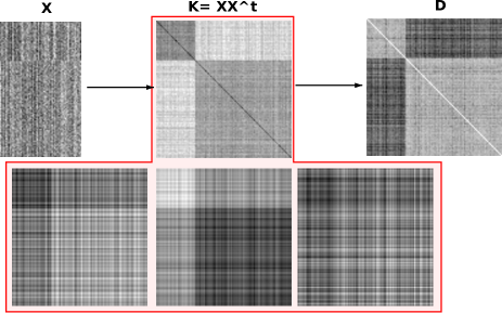
Figure 2: Information loss that occurs by moving from vectors $X$ to pairwise distances $D$. By moving from $X$ to pairwise similarities $K$, information about rotation of the vectors is lost, by moving from $K$ to $D$, information about translation is lost. One can reconstruct a whole equivalence class of $K$ matrices (four examples are bordered in red) from one distance matrix $D$, i. e. the reconstruction of a similarity matrix $K$ from $D$ is not unique, as there is a surjective mapping from a set of $K$ matrices to $D$.

Translation-invariant Wishart-Dirichlet Cluster Process:

A method which works directly on distances has been discussed in ([1],[32]) as an extension of the Wishart-Dirichlet Cluster Process. These methods cluster static distance data, and no access to vectorial data is required. The model presented in [32] tackles the problem if we do not directly observe $K$, but only a matrix of pairwise Euclidean distances $D$. In the following, the assumption is that the (suitably pre-processed) matrix $D$ contains squared Euclidean distances with components

$$D_{ij}=K_{ii}+K_{jj}-2K_{ij}.$$ (6)

A squared Euclidean distance matrix $D$ is characterized by the property of being of negative type, which means that $\boldsymbol{x}^{t}D\boldsymbol{x}=-\frac{1}{2}\boldsymbol{x}^{t}K\boldsymbol{x}<0$ for any $\boldsymbol{x}:\boldsymbol{x}^{t}\boldsymbol{1}=0$. This condition is equivalent to the absence of negative eigenvalues in $K_{c}=QKQ=-\frac{1}{2}QDQ$. The distribution of $D$ has been formally studied in [18], Eq. (3.2), where it was shown that if $K$ follows a standard Wishart generated from an underlying zero-mean Gaussian process, ${K}\sim\mathcal{W}_{d}(\Sigma_{B})$, $-D$ follows a generalized Wishart distribution, $-{D}\sim\mathcal{W}(\boldsymbol{1},2\Sigma_{B})=\mathcal{W}(\boldsymbol{1},-\Delta)$ defined with respect to the transformation kernel $\mathbb{K}=\boldsymbol{1}$, where $\Delta_{ij}={\Sigma_{B}}_{ii}+{\Sigma_{B}}_{jj}-2{\Sigma_{B}}_{ij}$. To understand the role of the transformation kernel it is useful to introduce the notion of a generalized Gaussian distribution with kernel $\mathbb{K}=\boldsymbol{1}$: $X\sim N(\boldsymbol{1},\boldsymbol{\mu},\Sigma)$. For any transformation $L$ with $L\boldsymbol{1}=0$, the meaning of the general Gaussian notation is: $LX\sim N(L\boldsymbol{\mu},L\Sigma L^{t})$. It follows that under the kernel $\mathbb{K}=\boldsymbol{1}$, two parameter settings $(\boldsymbol{\mu}_{1},\Sigma_{1})$ and $(\boldsymbol{\mu}_{2},\Sigma_{2})$ are equivalent if $L(\boldsymbol{\mu}_{1}-\boldsymbol{\mu}_{2})=\boldsymbol{0}$ and $L(\Sigma_{1}-\Sigma_{2})L^{t}=0$, i.e. if $\boldsymbol{\mu}_{1}-\boldsymbol{\mu}_{2}\in\boldsymbol{1}$, and $(\Sigma_{1}-\Sigma_{2})\in\{\boldsymbol{1}_{n}\boldsymbol{v}^{t}+\boldsymbol{v}\boldsymbol{1}_{n}^{t}:\boldsymbol{v}\in\mathbb{R}^{n}\}$, a space which is usually denoted by $\text{ sym}^{2}(\boldsymbol{1}\otimes\mathbb{R}^{n})$. It is also useful to introduce the distributional symbol $K\sim\mathcal{W}(\mathbb{K},\Sigma)$ for the generalized Wishart distribution of the random matrix ${K}=XX^{t}$ when $X\sim N(\mathbb{K},\boldsymbol{0},\Sigma)$. The key observation in [18] is that $D_{ij}=K_{ii}+K_{jj}-2K_{ij}$ defines a linear transformation on symmetric matrices with kernel $\text{ sym}^{2}(\boldsymbol{1}\otimes\mathbb{R}^{n})$ which implies that the distances follow a generalized Wishart distribution with kernel $\boldsymbol{1}$: $-{D}\sim\mathcal{W}(\boldsymbol{1},2\Sigma_{B})=\mathcal{W}(\boldsymbol{1},-\Delta)$ and

$$\textstyle\Delta_{ij}=\Sigma_{B_{ii}}+\Sigma_{B_{jj}}-2\Sigma_{B_{ij}}.$$ (7)

In the multi-dimensional case with spherical within- and between covariances we generalize the above model to Gaussian random matrices $X\sim N(\boldsymbol{\mu},\Sigma_{B}\otimes I_{d})$. Note that the $d$ columns of this matrix are i.i.d. copies. The distribution of the matrix of squared Euclidean distances $D$ then follows a generalized Wishart with $d$ degrees of freedom $-{D}\sim\mathcal{W}_{d}(\boldsymbol{1},-\Delta)$. This distribution differs from a standard Wishart in that the inverse matrix $W=\Sigma_{B}^{-1}$ is substituted by the matrix $\widetilde{W}=W-(\boldsymbol{1}^{t}W\boldsymbol{1})^{-1}W\boldsymbol{1}\boldsymbol{1}^{t}W$ and the determinant $|\cdot|$ is substituted by a generalized $\det(\cdot)$-symbol which denotes the product of the nonzero eigenvalues of its matrix-valued argument (note that $\widetilde{W}$ is rank-deficient). The conditional probability of a partition then reads

$$\begin{split}&P(B|D,\bullet)\textstyle\propto\mathcal{W}(-D|\boldsymbol{1},-\Delta)\cdot P_{n}(B|\xi,k)\\ &\textstyle\propto\det(\widetilde{W})^{\frac{d}{2}}\exp\left(\frac{d}{4}\text{tr}(\widetilde{W}D)\right)\cdot P_{n}(B|\xi,k).\end{split}$$ (8)

and the probability density function (which serves as likelihood function in the model) is then defined as

$$\textstyle f(D)\propto\det(\widetilde{W})^{\frac{d}{2}}\exp{\left(\frac{d}{4}\operatorname{tr}{(\widetilde{W}D)}\right)}.$$ (9)

Note that in spite of the fact that this probability is written as a function of $W=\Sigma_{B}^{-1}$, it is constant over all choices of $\Sigma_{B}$ which lead to the same $\Delta$, i.e. independent under translations of the row vectors in $X$. For the purpose of inferring the partition $B$, this invariance property means that one can simply use a block-partition covariance model $\Sigma_{B}$ and assume that the (unobserved) matrix $K$ follows a standard Wishart distribution parametrized by $\Sigma_{B}$. We do not need to care about the exact form of $K$, since the conditional posterior for $B$ depends only on $D$. Extensive analysis about the influence of encoding the translation invariance into the likelihood versus the standard WD process and row-mean subtraction was conducted in [32].

3 A Time-evolving Translation-invariant Wishart-Dirichlet Process

In this section, we present a novel dynamic clustering approach, the time-evolving translation-invariant Wishart-Dirichlet process (Te-TiWD) for clustering distance data that is available at multiple time points. In this model, we assume that pairwise distance data $D_{t}$ with $1\leq t\leq T$ is available over $T$ time points. At every time point $t$ all objects are fully exchangeable, and the number of data points may differ at the different time points. This model clusters data points over multiple time points, allowing group memberships and the number of clusters to evolve over time by addition, deletion or change in existing clusters. The model is based on the static clustering model that was proposed in [32] which is not able to account for a time structure. Note that our model completely ignores any information about the identities of the data points across the time points, which makes it possible to cluster different objects over time. Table 1 summarizes notations which we will use in the following sections.

$D_{t}$	distance matrix at time point $t$ (cf. (6))
$\Delta_{t}$	$\Delta$ matrix at time point $t$ (cf. (7))
$B_{t}$	partition matrix at time point $t$
$k_{b_{t}}$	number of blocks $b_{t}$ present
	in the partition $B_{t}$
$n_{b_{t}}$	the size of block $b_{t}$
$n_{b_{t}}^{(-l)}$	size of block $b_{t}$ without object $l$
$n_{t}$	number of data points
	present at the $t$-th time point
$A_{t}$	$k_{b_{t}}\times k_{b_{t}}$ matrix
$A_{t_{ij}}$	the between-class variance of
	block $i$ and block $j$
$[B_{t}]_{t=1}^{T}$	is defined as $(B_{1},B_{2},...,B_{T})$
$[A_{t}]_{t=1}^{T}$	is defined as $(A_{1},A_{2},...,A_{T})$
$p([B_{t}]_{t=1}^{T})$	$=p(B_{1})p(B_{2}|B_{1})....p(B_{T}|B_{T-1})$
	defines a first-order Markov chain
$p([A_{t}]_{t=1}^{T})$	$=p(A_{1})p(A_{2}|A_{1})....p(A_{T}|A_{T-1})$
	defines a first-order Markov chain
$[B]_{t-}$	$B$ matrices at all time points
	except at time point $t$

Table 1: Notations used throughout this manuscript.

3.1 The Model

The aim of the proposed method is to cluster distance data $D_{t}$ at multiple time points, for $1\leq t\leq T$. For every time point under consideration, $t$, we obtain a distance matrix $D_{t}$ and we want to infer the partition matrix $B_{t}$, by utilizing the partitions from adjacent time points. By using information from adjacent time points, we expect better clustering results than clustering every time point independently. At every time point, the number of data points may differ, and some clusters may die out or evolve over time. The assumptions on the data are the following:

Assumption 1

Given a partition $B_{t}$, a sequence of the assumed underlying $n_{t}$-dimensional vectorial observations $x_{t_{i}}\in\mathbb{R}^{n_{t}}$, $i=1,...,d_{t}$, are arranged as columns of the $(n_{t}\times d_{t})$ matrix $X_{t}$, i.e. $x_{t_{1}},...,x_{t_{d_{t}}}\hskip 2.84526pt\begin{subarray}{c}i.i.d\\ \sim\end{subarray}\hskip 2.84526pt{\mathcal{N}}(0,\Sigma_{B_{t}})$, with covariance matrix

$$\Sigma_{B_{t}}=\alpha I_{n_{t}}+\Sigma_{A_{t}}.$$ (10)

Covariance matrix $\Sigma_{B_{t}}$.

In the static clustering method, the underlying vectorial data was assumed to be distributed according to a Gaussian distribution with mean $0$, $x_{1},...,x_{d}\hskip 2.84526pt\begin{subarray}{c}i.i.d\\ \sim\end{subarray}\hskip 2.84526pt{\mathcal{N}}(0,\Sigma_{B})$ with $\Sigma_{B}:=\alpha I_{n}+\beta B$, (cf. (3)), where $\beta B$ describes the between class covariance matrix. As $\beta$ denotes a scalar, all clusters in the static clustering are equidistant (as demonstrated in left of Fig. 3). To model time evolving data, we need a more flexible between-class covariance matrix $\Sigma_{A_{t}}$ which allows that cluster centroids have different distances to each other. These full $\Sigma_{A_{t}}$ matrices are necessary for a time-evolving clustering model, as the clusters are coupled over the different time-points due to the geometric information of the clusters, and this coupling can only be captured by modeling a richer covariance. Hereby $\Sigma_{A_{t}}\in\mathbb{R}^{(n_{t}\times n_{t})}$ is obtained in the following way

$$\Sigma_{A_{t}}=Z_{t}A_{t}Z_{t}^{T}$$ (11)

with $Z_{t}\in\{0,1\}^{n_{t}\times k_{b_{t}}}$. The matrix $Z_{t}$ associates an object with one out of $k_{b_{t}}$ clusters. As every object can only belong to exactly one cluster, $Z_{t}$ has a single element of $1$ per row. In Fig. 3 we demonstrate examples of $\beta B$ and $\Sigma_{A_{t}}$ as well as the corresponding cluster arrangements which the matrices imply.

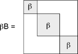
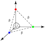
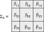
Figure 3: Different models for clustering. Left: example of the block diagonal structure of $\beta B$ for three blocks, all cluster centroids must be equidistant. Right: example of the full covariance matrix $\Sigma_{A_{t}}$ (for better readability, we drop the time index $t$ in the figure), which allows differing distances between cluster centroids.

Note that $\Sigma_{A_{t}}$ is a more general version of $\beta B$:

Lemma 1

$\Sigma_{A_{t}}=\beta B$      iff       $A_{t_{ij}}=\left\{\begin{array}[]{cc}0&\,\,\textnormal{if}\,\,i\neq j\\ \beta&\textnormal{if}\,\,i=j\end{array}\right..$

Prior over the block matrices $B_{t}$.

The prior over the block matrices $B_{t}$ is defined in the following way. The prior for $B_{t}$ in one epoch is the Dirichlet-Multinomial prior over partitions as in (1). Using the definition of the conditional prior over clusters as defined in [2], we extend this idea to the prior over partitions. In a generative sense, the same idea is used to generate a labeled set of partitions and then we forget the labels to get a distribution over partitions. By $n^{t}_{b_{t-1}}$ we denote the size of block ${b_{t-1}}$ if the corresponding block is present at time point $t$ as well. We consider the following generative process for a finite dynamic mixture model with $k$ mixtures (cf. [2], Eqs. (4.5), (4.6) and (5.9)): for each time point $t$, we generate mixing proportions $\pi_{t}=(\pi_{t1},...,\pi_{tk})$ from a symmetric Dirichlet distribution $\textnormal{Dir}(\xi/k+n_{t-1},...,\xi/k+n_{t-1})$. As in the static case, we generate a label sequence from a multinomial distribution and forget the labels introducing the random partition $B_{t}$. Integrating out $\pi_{t}$, the conditional distribution for Dirichlet-Multinomial prior over partitions, given the partitions in the previous time point $(t-1)$, can be written as:

$$P_{n_{t}}(B_{t}|B_{t-1},\xi,k)=\frac{k!}{(k-k_{B_{t}})!}\frac{\Gamma(\xi+n_{t-1})\prod_{b_{t}\in B_{t}}\Gamma(n^{t}_{b_{t-1}}+\xi/k+n_{b_{t}})}{\Gamma(n_{t}+\xi+n_{t-1})\prod_{b_{t}\in B_{t}}\Gamma(\xi/k+n^{t}_{b_{t-1}})}$$ (12)

Note that (12) defines a partition process as described in section 2 with $P_{n_{t}}$ being the marginal distribution of $P_{n_{t-1}}$, and it also is an exchangeable process, as each $P_{n_{t}}$ is invariant under permutation of object indices.

Prior over $A_{t}$.

The prior over the $A_{t}$ matrices is given by a Wishart distribution, $P(A_{t}|A_{t-1})\sim\mathcal{W}_{d}(A_{t}|A_{t-1})$ and $S_{0}:=P(A_{1})=\mathcal{W}_{d}(A_{1}|I_{k_{b_{1}}})$. The degrees of freedom $d$ influences the behavior of the Wishart distribution: a low value for $d$ allows drastic changes in the clustering structure, a high value for $d$ allows fewer changes. We also have to consider that the size of $A_{t-1}$, $A_{t}$ and $A_{t+1}$ might differ, as it is possible that the number of clusters in every epoch is different. Therefore, we consider the following two cases:

• if there are more blocks at time $t-1$ than at time $t$, i. e. $k_{b_{t-1}}>k_{b_{t}}$:
  delete corresponding rows and columns in $A_{t-1}$. With $A^{\prime}_{t-1}$ we denote the “reduced” matrix. Then it holds that $A_{t}\sim\mathcal{W}_{d}(A^{\prime}_{t-1})$
  

• if there are fewer blocks at time $t-1$ than at time $t$, i. e. if $k_{b_{t-1}}<k_{b_{t}}$:
  first, draw a $k_{b_{t-1}}\times k_{b_{t-1}}$ matrix $A^{\prime}_{t}$ from $A^{\prime}_{t}\sim\mathcal{W}_{d}(A_{t-1})$. Second, augment as many new rows and columns as needed to obtain the full positive definite $(k_{b_{t}})\times(k_{b_{t}})$ matrix $A_{t}$. We can draw the additional rows and columns of $A_{t}$ in the following way (see [5] for details):

  $$A_{t}=\left(\begin{matrix}A_{11}A_{12}\\ A_{21}A_{22}\end{matrix}\right)$$ (13)

  with $A_{11}:=A^{\prime}_{t}\in\mathbb{R}^{(k_{b_{t-1}})\times(k_{b_{t-1}})}$, $A_{21}\in\mathbb{R}^{1\times(k_{b_{t-1}})}$, $A_{12}\in\mathbb{R}^{(k_{b_{t-1}})\times 1}$ and $A_{22}\in\mathbb{R}$. One obtains $A_{12}$, $A_{21}$ and $A_{22}$ in the following way:

  $$\begin{split}A_{12}|A_{11}&\sim&\mathcal{N}(0,A_{11}\otimes s)\\ A_{22.1}&\sim&\mathcal{W}_{1}(d-k_{b_{t}},s)\\ A_{22}&=&A_{22.1}+A_{21}A_{11}^{-1}A_{12}\end{split}$$ (14)

  where $s$ denotes a scalar value and $d$ the degrees of freedom of the Wishart distribution $\mathcal{W}_{d}(A_{t-1})$.

A graphical depiction of the generative model of Te-TiWD is given in Fig. 4.

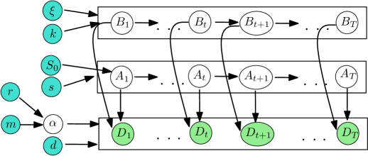
Figure 4: Depiction of the generative model of Te-TiWD with all hyper-parameters and parameters. Shaded circles correspond to fixed or observed variables, unshaded to latent variables. Arrows that point to a box mean that the parameters apply to all the variables inside the box, whereas arrows that directly point to a variable only apply to that single variable. $D_{t}$ denote the distance matrices observed at different points in time, $B_{t}$ denote the inferred partitions and $A_{t}$ the between class covariance matrices at different time points $1\leq t\leq T$.

Posterior over $B_{t}$ and $A_{t}$.

With the likelihood for every time point, analogous to Eq. (9), and the prior over $A_{t}$ and $B_{t}$, we can now write down the equations for the posterior over $B_{t}$ and $A_{t}$ for all time points $t\in\{1,2,...,T\}$:

$$p([B_{t}]_{1}^{T},[A_{t}]_{1}^{T}|[D_{t}]_{1}^{T},\bullet)\propto\prod_{t=1}^{T}{\mathcal{W}}_{d}^{-}(D_{t}|\textbf{1},\Delta_{t})P([B_{t}]_{1}^{T})P([A_{t}]_{1}^{T})$$ (15)

$$=\prod_{t=1}^{T}\det(\widetilde{W_{t}})^{\frac{d_{t}}{2}}\exp{\left(\frac{d_{t}}{4}\operatorname{tr}{(\widetilde{W_{t}}D_{t})}\right)}P([B_{t}]_{1}^{T})P([A_{t}]_{1}^{T})$$ (16)

with $\widetilde{W_{t}}:=W_{t}-(\boldsymbol{1}^{T}W_{t}\boldsymbol{1})^{-1}W_{t}\boldsymbol{1}\boldsymbol{1}^{T}W_{t}$, where $W_{t}:=\Sigma_{B_{t}}^{-1}$ (cf. (LABEL:eq:distrD) and (9)).

3.1.1 MCMC sampling for posterior inference.

For applying MCMC sampling to sample from the posterior, we look at the conditional distributions. Consider the conditional distributions at each time point $t$:

$$\begin{split}&p(B_{t},A_{t}|D_{t},[B]_{t-},[A]_{t-},\bullet)\propto\\ &\mathcal{W}_{d}^{-}(D_{t}|\textbf{1},\Delta_{t})P(B_{t}|B_{t-1})P(B_{t+1}|B_{t})P(A_{t}|A_{t-1})P(A_{t+1}|A_{t})\end{split}$$ (17)

Posterior sampling for $B_{t}$.

The posterior sampling involves sampling assignments. As we are dealing with non-conjugate priors in (17), we use a Gibbs sampling algorithm with $m$ auxiliary variables as presented in [20]. We consider the infinite model with $k\rightarrow\infty$. The aim is to assign one object $l$ in epoch $t$ to either an existing cluster $c$, a new cluster that exists at epoch $t-1$ or epoch $t+1$ or a totally new cluster. The prior probability that object $l$ belongs to an exisiting cluster $c$ at time point $t$ is

$$P(l=c|B_{t-1})P(B_{t+1}|B_{t})\propto n_{c_{t-1}}+n_{c_{t}}^{(-l)})\cdot\frac{n_{c_{t+1}}}{n_{c_{t}}^{(-l)}}.$$ (18)

There exist four different prior probabilities of an object $l$ belonging to a new cluster $c_{new}$ at time point $t$, which are summarized in table 2.

$\boldmath{c_{\textnormal{new}}}$ exists at	$\bf P(l=c_{new}|B_{t-1})P(B_{t+1}|B_{t})$
both time points $t-1$ and $t+1$:	$\propto(n_{c_{t-1}}\cdot\frac{\xi}{m})\cdot n_{c_{t+1}}$	(19)
time point $t-1$ but not at time point $t+1$:	$\propto\frac{\xi}{m}\cdot n_{c_{t-1}}$	(20)
time point $t+1$ but not at time point $t-1$	$\propto\frac{\xi}{m}\cdot n_{c_{t+1}}$	(21)
neither $t-1$ nor $t+1$,	$\propto\frac{\xi}{m}$	(22)
(i.e. $l$ belongs to a completely new cluster)

Table 2: Table of prior probabilities.

Metropolis-Hastings update steps.

In every time point, we need to sample $\beta$ values in the between-class variance matrix $\Sigma_{A_{t}}$. To find the $\beta$ values within one epoch, we sample the whole “new” $A_{t}$ matrix, denoted by $A_{t_{new}}$, with a Metropolis-Hastings algorithm (see [24]). With $A_{t_{old}}$ we denote the initial $A_{t}$ matrix. As proposal distribution we chose a Wishart distribution, and for the prior we chose a Wishart distribution as well, leading to $P(A_{t_{new}}|A_{t_{old}})\sim\mathcal{W}(A_{t_{new}}|A_{t_{old}})$ and $P(A_{t_{new}})\sim\mathcal{W}(A_{t_{new}}|I_{k_{b_{t}}}).$

Hyperparameters and Initialization.

Our model includes the following hyperparameters: the scale parameter $\alpha$, the number $k$ of clusters, the Dirichlet rate $\xi$, the degrees of freedom $d$ and a scale parameter $s$. The model is not sensitive to the choice of $s$, and we fix $s$ to 1. $\alpha$ is sampled from a Gamma distribution with shape and scale parameters $r$ and $m$. For the number $k$ of clusters, our framework is applicable to two scenarios: we can either assume $k=\infty$ which results in the CRP model, or we fix $k$ to a large constant which can be viewed as a truncated Ewens process. As the model does not suffer from the label switching problem, initialization is not a crucial problem. We initialize the block size with size 1, i. e. we start with one cluster for all objects. The Dirichlet rate $\xi$ only weakly influences the likelihood, and the variance only decays with $1/\log(n_{t})$ (see [11]). In practice, we should not expect to reliably estimate $\xi$. Rather, we should have some intuition about $\xi$, maybe guided by the observation that under the Ewens process model the probability of two objects belonging to the same cluster is $1/(1+\xi)$. We can then either define an appropriate prior distribution, or we can fix $\xi$. Due to the weak effect of $\xi$ on conditionals, these approaches are usually very similar. The degrees of freedom $d$ can be estimated by the rank of $K$, if it is known from a pre-processing procedure. As $d$ is not a very critical parameter (all likelihood contributions are basically raised to the power of $d$), $d$ might also be used as an annealing-type parameter for freezing a representative partition in the limit for $d\rightarrow\infty$.

Pseudocode.

A pseudocode of the sampling algorithm is given in Algorithm 1.

  for  $i=1$ to iteration do

     for  $t=1$ to $T$ do

        for  $j=1$ to $n_{t}$ do

           Assign one object to an existing cluster or a new one using Eqs. (17)-(2)Update $k_{b_{t}}$

        end for

     end for

     for  $t=1$ to $T$ do

        Sample new $A_{t}$ matrix using Metropolis-Hastings

     end for

  end for

Algorithm 1 Pseudocode Te-TiWD

Complexity.

We define one sweep of the Gibbs sampler as one complete update of $(B_{t},A_{t})$. The most time consuming part in a sweep is the update of $B_{t}$ by re-estimating the assignments to blocks for a single object (characterized by a row/column in $D_{t}$), given the partition of the remaining objects. Therefore we have to compute the membership probabilities in all existing blocks (and in a new block). Every time a new partition is analyzed, a naive implementation requires $O(n^{3})$ costs for computing the determinant of $\tilde{W}_{t}$ and the product $\tilde{W}_{t}D_{t}$. In one sweep we need to compute $k_{b_{t}}$ such probabilities for $n_{t}$ objects, summing up to costs of $O(n^{4}k_{b_{t}})$. This suggests that the scalability to large datasets can pose a problem. In this regard we plan to address run time in future work by investigating the potential of variational methods, parallelizing the MCMC sampler and by updating parameters associated with multiple time points simultaneously.

Identifiability of clusters.

In some applications, it is of interest to identify and track clusters over time. For example by grouping newspaper articles into topics it might be interesting to know which topics are present over a long time period, when a new topic becomes popular and when a former popular topic dies out. Due to the translation-invariance of our novel longitudinal model, we additionally need a cluster mean to be able to track clusters over the time course. To estimate the mean of the clusters we propose to embed the “overall” data matrix $D^{*}\in\mathbb{R}^{N\times N}$ with $N:=\sum_{t=1}^{T}n_{t}$ that contains the pairwise distances between all objects over all time points into a vector space, using kernel PCA. We first construct a positive semi-definite matrix $K^{*}$ which fulfills $D^{*}_{ij}=K^{*}_{ii}+K^{*}_{jj}-2K^{*}_{ij}$. For correcting $K^{*}$, we compute the centered matrix $K^{*}_{c}=Q^{*}K^{*}Q^{*}$ with $Q^{*}_{ij}=\delta_{ij}-\frac{1}{N}$. As a next step, we compute the eigenvalue decomposition of $K^{*}_{c}$, i.e. $K^{*}_{c}=V\Lambda V^{T}$ and then project on the principal axes $X^{*}=V\Lambda^{\frac{1}{2}}$, i.e. we use the principal components as coordinate axes. By embedding the distances $D^{*}$ into a vector space, the underlying block structure might be distorted (see Fig. 2). As our aim is to find the underlying block structure, it is hence infeasible to embed the data for clustering. But, for tracking the clusters, we just need to find the mean of an already inferred block structure, i.e. we embed the data not for grouping data points, but for finding a mean of an already assigned partition that allows us to track the clusters over time. We embed all objects together and choose the same orthogonal transformations for all objects, which enables identifiability of cluster means over the time course. This preprocessing step is only necessary if one is interested in the identifiability of clusters, and $X^{*}$ needs only to be computed once outside the sampling routine. Since computing $X^{*}$ is computationally expensive, it is done only once as a preprocessing step if required. Computing $X^{*}$ within the sampling routine would slow down our sampler significantly.

4 Experiments

4.1 Synthetic Experiments

4.1.1 Well separated clusters.

In a first experiment, we test our method on simulated data. We simulate data in two ways, first we generate data points accordingly to the model assumptions, and secondly we generate data independent of the model assumptions. We start with a small experiment where we consider five time points each with 20 data points per time point in 100 dimensions, i. e. we consider a small data set size and large dimension problem.

Data generation.

The data is generated (according to the model assumptions) in the following way: for the first time point, a random block matrix $B_{1}$ of size $n_{1}=20$ is sampled with $k_{b_{1}}=3$ (i.e. we generate 3 blocks at time point 1). A $k_{b_{1}}\times k_{b_{1}}$ matrix $A_{1}$ is sampled from $\mathcal{W}_{d}(I_{k_{b_{1}}})$ and $B_{1}$ is filled with the corresponding $\beta$ values from $A_{1}$, which leads to the $n_{1}\times n_{1}$ matrix $\Sigma_{K_{1}}$. Next, $d_{1}=100$ samples from $\mathcal{N}(0_{n},\Sigma_{B_{1}})$ are drawn with $\Sigma_{B_{1}}=\alpha I_{n_{1}}+\Sigma_{A_{1}}$, where $\alpha=2$, and stored in the $(n_{1}\times d_{1})$ matrix $X_{1}$. By choosing $\alpha=2$, we create well separated clusters. The similarity matrix $K_{1}=X_{1}X_{1}^{T}$ is computed and squared distances are stored in matrix $D_{1}$. For the following time points $t>1$, the partition for the block matrix $B_{t}$ of size $n_{t}$ is drawn from a Dirichlet-Multinomial distribution, conditioned on the partition at time point $t-1$. A new $A_{t}$ matrix is sampled from $\mathcal{W}_{d}(A_{t-1})$. If the number of blocks in time points $t$ and $t-1$ are different, we sample $A_{t}$ according to Eq. (14). $d_{t}$ samples from $\mathcal{N}(0_{n_{t}},\Sigma_{B_{t}})$ are drawn with $\Sigma_{B_{t}}=\alpha I_{n_{t}}+\Sigma_{A_{t}}$. The pairwise distances are stored in the matrix $D_{t}$. A PCA projection of this data is shown in Fig. 5 for illustration.

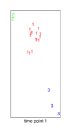
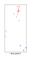
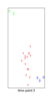
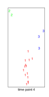
$\xrightarrow{\textnormal{time}}$ $\xrightarrow{\textnormal{time}}$ $\xrightarrow{\textnormal{time}}$ $\xrightarrow{\textnormal{time}}$

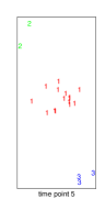
Figure 5: PCA projections of five time points with three well separated clusters per time point. Numbers and colors correspond to true labels.

Experiments.

We perform four illustrative experiments for well-separated data:

1. 500 Gibbs sweeps are computed for the Te-TiWD cluster process (after a burn-in phase of 250 sweeps). We check convergence of the algorithm by analyzing the trace of the number of blocks $k_{b_{t}}$ during sampling. On this trace plot we observe after how many sweeps the sampler stabilizes (the number of sweeps depends on the size of the data set). We observe a remarkable stability of the sampler (compared to the usual situations in traditional mixture models), which follows from the fact that no label-switching can appear. Finally, we perform an annealing procedure to freeze a certain partition. Here, $d$ is used as an annealing-type parameter for freezing a representative partition in the limit $d\rightarrow\infty$. On a standard computer, this experiment took roughly 4 minutes, and the sampler stabilizes after roughly 50 sweeps. As the ground truth is known, we can compute the adjusted rand index as an indicator for the accuracy of the Te-TiWD model. We repeat the clustering process 50 times. The result is shown in form of a box plot (Te-TIWD) in Fig. 6.

2. In order to compare the performance of the time-evolving model (Te-TiWD) to baseline models, we also run the static probabilistic clustering process as well as hierarchical clustering models (Ward, complete linkage and single linkage) on every time point separately and compute the averaged accuracy over all time points. For the comparison to the static probabilistic method [32], we use the same set-up as for Te-TiWD, we run 500 Gibbs sweeps with a burn-in phase of 250 sweeps and repeat it for 50 times. For the hierarchical methods, the resulting trees are cut at the number of clusters found by the nonparametric probabilistic model. Accuracy is computed for every time point separately, and then averaged over all time points. In this scenario, the static clustering models performs almost as well as the time-evolving clustering, see Fig. 6, as expected in such a setting where all groups are well separated at every single time point.

3. As a further comparison to a baseline dynamic clustering model, we embed the distances into a Euclidean vector space and run a Gaussian dynamic clustering model (Te-Gauss) on the embedded vectorial data. As the clusters are well separated, embedding the data and clustering on vectors works well, as shown in box plot “Te-Gauss” in Fig. 6.

4. As a last comparison we evaluate a pooled clustering over all time points. For this experiment, we not only need the pairwise distances at every single time point, but also the pairwise distances of objects across all time points. The number of sweeps and repetitions remains the same as in the experiments above. We conduct one clustering over all objects of all time points, and after clustering, we extract the objects belonging to the same time point and compute the rand index on every time point separately. This experiment shows worse results (see box plot “pooled” in Fig. 6), which can be explained as follows: by combining all time points to one data matrix, new clusters over all time points are found, this means clusters are shifted and objects over time are grouped together, introducing new clusters by reforming boundaries of old clusters. These new clusters inhibit objects to group together which would group together at single time points, destroying the underlying “true” cluster structure.

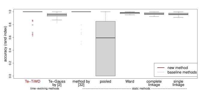
Figure 6: We compare our new dynamic model (Te-TiWD) with baseline methods: static clustering as in [32], combined clustering over all time points (pooled), a Gaussian time-evolving clustering model (Te-Gauss) as well as to Ward, complete linkage and single linkage. In this experiment with three well separated clusters per time point, all methods perform very well, except for pooling the data.

4.1.2 Highly overlapping clusters.

For a second experiment, we generated data in a similar way as above, but this time we create 5 highly overlapping clusters each with 200 data points per time point in 40 dimensions. A PCA projection of this data is shown in Fig. 8. On a standard computer, this experiment took roughly 3 hours, and the sampler stabilizes after roughly 500 sweeps. Again, we compare the performance of the translation-invariant time-evolving clustering model with static state-of-the-art probabilistic and hierarchical clustering models which cluster on every time point separately and a time-varying Gaussian clustering model on embedded data (Te-Gauss). For highly overlapping clusters, the new dynamic clustering model outperforms the static probabilistic clustering model [32], and the hierarchical models (Ward, complete linkage, single linkage) fail completely. Further, our new model Te-TiWD outperforms the dynamic, vectorial clustering model (Te-Gauss), demonstrating that embedding the data into a Euclidean vector space yields worse results than working on the distances directly. We tested the statistical significance with the Kruskal-Wallis rank-sum test and the Dunn post test with Bonferroni correction for pairwise analysis. These tests show that Te-TiWD performs significantly better than all clustering models we compared to. Results are shown in Fig. 7.

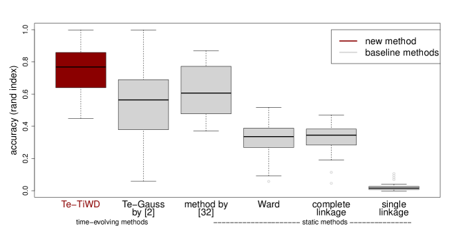
Figure 7: We compare our new model (Te-TiWD) with baseline methods on synthetic data for five highly overlapping clusters. Our model significantly outperforms all baseline methods.

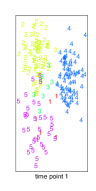
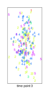
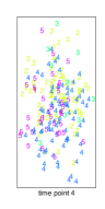
$\xrightarrow{\textnormal{time}}$ $\xrightarrow{\textnormal{time}}$ $\xrightarrow{\textnormal{time}}$ $\xrightarrow{\textnormal{time}}$

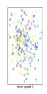
Figure 8: PCA projections of five time points of simulated data with five highly overlapping clusters. Numbers and colors correspond to true labels.

4.1.3 Data generation independent of model assumptions.

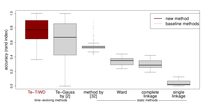
Figure 9: We compare our new model (Te-TiWD) with baseline methods on synthetic data which is generated independent of the model assumptions for five highly overlapping clusters. We observe that our method significantly outperforms all baseline methods.

We also generate data in a second way which is independent of the model assumptions to demonstrate that the performance of our model Te-TiWD is independent of the way the data was generated. To demonstrate this, we repeat the case of highly overlapping clusters over 5 time points and generate data in the following way: dynamic Gaussian clusters are generated over a period of 5 time points. At each time point five clusters are generated. 200 data points are available at every time point and randomly split into 5 parts, every part representing the number of data points per cluster. For consecutive time points, the number of data points per cluster is sampled from a Dirichlet-Multinomial distribution. Every cluster is sampled from a Gaussian distribution with a large variance, resulting in highly overlapping clusters. Between time steps, the cluster centers move randomly, with relocations sampled from the same distribution. Finally, at every time point, the model-based pairwise distance matrix $D_{t}$ is computed, resulting in a series of moving distance matrices. On this second synthetic data set, Te-TiWD performs significantly better than all baseline methods as well, as shown in Fig. 9. Note that for the comparison with the Gaussian dynamic clustering model (Te-Gauss) we first embed the distances $D_{t}$ into vectorial data $X_{t}^{*}$ and do not work on the simulated vectorial data directly, to obtain a fair comparison.

4.2 Analysis of Brain Cancer Patient based on Electronic Health Records (EHR)

We apply our proposed model to a dataset of clinical notes from brain cancer patients at Memorial Sloan Kettering Cancer Center (MSKCC). Brain cancer patients make up 1.4% of all cancer patients, annually. Survival is highly variable, depending on age, gender, cancer subtype, and progression when caught, but on average 33% of patients survive the first five years.
As a first step, we partition a total of 195,297 sentences from 3,403 electronic health records (EHR) from 704 MSKCC brain cancer patients into groups of similar vocabulary. This is done by treating sentences as binary vectors with non-zero entries corresponding to vocabulary, and obtaining a similarity measure using ranked neighborhood comparisons [31]. Sentences are clustered using this similarity measure with the Louvain method [8]. Using these sentence clusters as features, we obtain patient similarities with the same ranked neighborhood comparison method. We partition the patients documents into windows of one year each, and obtain three time points where enough documents are available to compute similarities between patients. At each year, we represent a patient with a binary vector whose length is the number of sentence clusters. A non-zero entry corresponds to an occurrence of that sentence cluster in the patient’s corpus during the specified time period.

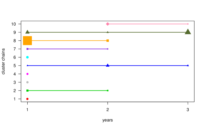
Figure 10: Clusters over all 3 years of brain cancer patients. We find ten different cluster chains where 2 remain over al three years, 3 vanish after the second year and one new cluster comes up in year 2 and remains in the third year. Size of the tokens denote the cluster size, i.e. the number of patients per cluster. Note that patients can change clusters, so a cluster decreasing in size or disappearing does not necessarily mean those patients die or leave the hospital.

In the first year, we have 704 patients, in the second year 170 and in the third year 123 patients. This data set has specific features which make our model particularly suitable to cope with this kind of data. First, the number of patients differs in every year. Second, patients disappear over the time course, either due to death or due to leaving the hospital. Third, patients do not necessarily need to have a document every year, so a patient can be absent from year 2 and appear in year 3. This gap occurred a total of 31 times in our data set. This is why our flexible model is very well suited for this problem, as the model can deal with changing numbers of objects and changing number of clusters in every year, clusters can disappear or reappear, as well as patients. The result of our clustering model is shown in Fig. 10. On a standard computer, this experiment took roughly 6 hours, and the sampler stabilizes after roughly 500 sweeps.
We observe ten different cluster chains over the time series. Note that patients can switch cluster chains over the years, as the tumor progresses, the status of the patient may change, resulting in more similarities to a different cluster chain than the year before. To analyze the results of the method, we will discuss the most and least deadly clusters in more detail, as analyzing all subtleties between clusters would be out of the scope of this paper.
Cluster chain 1 is the most deadly cluster, with a death rate of 80%. Additionally, it only appears in the first year. Word clouds representing the sentence clusters of this patient group are shows in Fig. 11. We can see that these patients are having seizures which indicates that the brain cancer is especially malicious. They also show sentence clusters about two types of blood cancers, b cell and mantle cell lymphoma, and prescription of cytarabine, which treats these cancers. This combination of blood and brain cancers could explain why this cluster chain is so deadly.

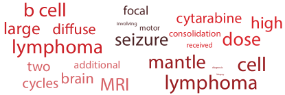
Figure 11: Word clouds representing five sentence clusters that are observed in patients from cluster chain 1, the most deadly cluster. They describe patients that have blood cancers (lymphomas) in addition to brain cancer.

Cluster chain 5 is the least deadly chain with a death rate of 42%. Word clouds representing sentence clusters for this patient group are show in Fig. 12. These clusters consist of mainly ”follow-up” language, such as checking the patients’ gait, speech, reflexes and vision. The sentence clusters appear to indicate positive results, e.g. ”Normal visual fields are intact”, and ”Patient denies difficulty with speech, language, balance or gait” are two prototype sentences representing two sentence clusters that appear in this chain. Furthermore, there is a sentence cluster with prototype sentence ”no evidence for progression,” indicating that these patient’s cancers are in a manageable state.

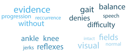
Figure 12: Word clouds representing four sentence clusters that are observed in patients from cluster chain 5, the most positive cluster. These sentence clusters are ”follow-up” language, such as checking reflexes or the ability to walk and see well. This indicates that the patients are in a relatively stable state under regular observation.

Modeling patients over time provides important insights for automated analyses and medical doctors, as it is possible to check for every patient how the state of the patient as represented by the cluster membership changes over time. Also, if a new patient enters the study, one can infer, based on similarity to other patients, how to classify and possibly treat this patient best or to suggest clinical trials for each patient. Such clustering methods therefore make an important step towards solving the technical challenges of personalized cancer treatment.

5 Conclusion

In this work, we propose a novel dynamic Bayesian clustering model to cluster time-evolving distance data. A probabilistic model that is able to handle non-vectorial data in form of pairwise distances has the advantage that there is no need to embed the data into a vector space. To summarize, our contributions in this work are five-fold: i) We develop a dynamic probabilistic clustering approach that circumvents the potentially problematic data embedding step by directly operating on pairwise time-evolving distance data. ii) Our model enables to track the clusters over time, giving information about clusters that die out or emerge over time. iii) By using a Dirichlet process prior, there is no need to fix the number of clusters in advance. iv) We test and validate our model on simulated data. We compare the performance of our new method with baseline probabilistic and hierarchical clustering methods. v) We use our model to cluster brain cancer patients into similar subgroups over a time course of three years. Dynamic partitioning of patients would play an important role in cancer treatment, as it enables inference from groups of similar patients to an individual. Such an inference can help medical doctors to adapt or optimize existing treatments, assign billing codes, or predict survival times for a patient based on similar patients in the same group.

Acknowledgments

We thank Natalie Davidson, Theofanis Karaletsos and David Kuo for helpful discussions and suggestions. JV and MK were partly funded through postdoctoral fellowships awarded by the Swiss National Science Foundation (SNSF; under PBBSP2_146758) and by the German Research Foundation (DFG; under Kl 2698/1-1 and VO 2003/1-1), respectively. We gratefully acknowledge funding from Memorial Sloan Kettering Cancer Center and the National Cancer Institute (grant 1R01CA176785-01A1). Access to patient data is covered under IRB Waiver #WA0426-13.

References

- [1] David Adametz and Volker Roth. Bayesian partitioning of large-scale distance data. In NIPS, pages 1368–1376, 2011.
- [2] Amr Ahmed and Eric Xing. Dynamic non-parametric mixture models and the recurrent Chinese restaurant process: with applications to evolutionary clustering. Proceedings of The Eighth SIAM International Conference on Data Mining (SDM), 2008.
- [3] T.W. Anderson. The non-central wishart distribution and certain problems of multivariate statistics. Ann. Math. Statist., 17(4):409–431, 1946.
- [4] Seema Bandyopadhyay and Edward J Coyle. An energy efficient hierarchical clustering algorithm for wireless sensor networks. In INFOCOM 2003. Twenty-Second Annual Joint Conference of the IEEE Computer and Communications. IEEE Societies, volume 3, pages 1713–1723. IEEE, 2003.
- [5] M. Bilodeau and D. Brenner. Theory of Multivariate Statistics. Springer, 1999.
- [6] D. Blei and M. Jordan. Variational inference for Dirichlet process mixtures. Bayesian Analysis, 1:121–144, 2006.
- [7] David M. Blei and Peter Frazier. Distance dependent chinese restaurant processes. Journal of Machine Learning Reseach, 12(12):2461–2488, 2011.
- [8] Vincent D Blondel, Jean-Loup Guillaume, Renaud Lambiotte, and Etienne Lefebvre. Fast unfolding of communities in large networks. Journal of Statistical Mechanics: Theory and Experimen, 2008.
- [9] M Cuturi and J-P Vert. A mutual information kernel for strings. In Proceedings of the International Joint Conference on Neural Network, 2004.
- [10] Michael B Eisen, Paul T Spellman, Patrick O Brown, and David Botstein. Cluster analysis and display of genome-wide expression patterns. Proceedings of the National Academy of Sciences, 95(25):14863–14868, 1998.
- [11] W.J. Ewens. The sampling theory of selectively neutral alleles. Theoretical Population Biology, 3:87–112, 1972.
- [12] T. S Ferguson. A bayesian analysis of some nonparametric problems. Annals of Statistics 1, pages 209–230, 1973.
- [13] Anil K. Jain. Data clustering: 50 years beyond k-means, 2008.
- [14] Anil K Jain and Richard C Dubes. Algorithms for clustering data. Prentice-Hall, Inc., 1988.
- [15] Daniel D Lee and H Sebastian Seung. Learning the parts of objects by non-negative matrix factorization. Nature, 401(6755):788–791, 1999.
- [16] C. Leslie, E. Eskin, A. Cohen, J. Weston, and W.S. Noble. Mismatch string kernel for discriminative protein classification. Bioinformatics, 1(1):1–10, 2003.
- [17] S.N. MacEachern. Estimating normal means with a conjugate-style Dirichlet process prior. Communication in Statistics: Simulation and Computation, 23:727–741, 1994.
- [18] P. McCullagh. Marginal likelihood for distance matrices. Statistica Sinica, 19:631–649, 2009.
- [19] P. McCullagh and J. Yang. How many clusters? Bayesian Analysis, 3:101–120, 2008.
- [20] R.M. Neal. Markov chain sampling methods for Dirichlet process mixture models. Journal of Computational and Graphical Statistics, 9:249–265, 2000.
- [21] Andrew Y Ng, Michael I Jordan, Yair Weiss, et al. On spectral clustering: Analysis and an algorithm. Advances in neural information processing systems, 2:849–856, 2002.
- [22] J. Pitman. Combinatorial stochastic processes. In J. Picard, editor, Ecole d’Ete de Probabilites de Saint-Flour XXXII-2002. Springer, 2006.
- [23] Gunnar Rätsch and Sören Sonnenburg. Accurate splice site prediction for caenorhabditis elegans. In Kernel Methods in Computational Biology, MIT Press series on Computational Molecular Biology, pages 277–298. MIT Press, 2004.
- [24] C.P. Robert and G. Casella. Monte Carlo Statistical Methods. Springer, 2005.
- [25] H Saigo, J-P Vert, N Ueda, and T Akutsu. Protein homology detection using string alignment kernels. Bioinformatics, 20(11):1682–1689, 2004.
- [26] Sören Sonnenburg, Gunnar Rätsch, and Konrad Rieck. Large scale learning with string kernels. In Léon Bottou, Olivier Chapelle, Dennis DeCoste, and Jason Weston, editors, Large Scale Kernel Machines, pages 73–103. MIT Press, Cambridge, MA., 2007.
- [27] M.S. Srivastava. Singular Wishart and multivariate beta distributions. Annals of Statistics, 31(2):1537–1560, 2003.
- [28] Michael Steinbach, George Karypis, Vipin Kumar, et al. A comparison of document clustering techniques. In KDD workshop on text mining, volume 400, pages 525–526. Boston, 2000.
- [29] Y. W. Teh, C. Blundell, and L. T. Elliott. Modelling genetic variations with fragmentation-coagulation processes. In Advances In Neural Information Processing Systems, 2011.
- [30] S. V. N. Vishwanathan, Nicol N. Schraudolph, Risi Kondor, and Karsten M. Borgwardt. Graph kernels. J. Mach. Learn. Res., 11:1201–1242, August 2010.
- [31] Julia E. Vogt. Unsupervised structure detection in biomedical data. IEEE/ACM Transactions on Computational Biology and Bioinformatics, 2015.
- [32] Julia E. Vogt, Sandhya Prabhakaran, Thomas J. Fuchs, and Volker Roth. The translation-invariant Wishart-Dirichlet process for clustering distance data. In ICML, pages 1111–1118, 2010.
- [33] Xiaojin Zhu, Zoubin Ghahramani, and John Lafferty. Time-sensitive dirichlet process mixture models. Technical report, Carnegie Mellon University, 2005.