Quantum theory of light scattering in a one-dimensional channel:
Interaction effect on photon statistics and entanglement entropy

Abstract

We provide a complete and exact quantum description of coherent light scattering in a one-dimensional multi-mode transmission line coupled to a two-level emitter. Using recently developed scattering approach we discuss transmission properties, power spectrum, the full counting statistics and the entanglement entropy of transmitted and reflected states of light. Our approach takes into account spatial parameters of an incident coherent pulse as well as waiting and counting times of a detector. We describe time evolution of the power spectrum as well as observe deviations from the Poissonian statistics for reflected and transmitted fields. In particular, the statistics of reflected photons can change from sub-Poissonian to super-Poissonian for increasing values of the detuning, while the statistics of transmitted photons is strictly super-Poissonian in all parametric regimes. We study the entanglement entropy of some spatial part of the scattered pulse and observe that it obeys the area laws and that it is bounded by the maximal entropy of the effective four-level system.

I Introduction

I.1 Overview of studies of scattering in one-dimensional channel with emitter

With current advances in experimental nanooptics, the problem of light scattering in quasi-one dimensional waveguides becomes an important cornerstone for understanding physics behind the light-matter interaction in a confined geometry. A number of recent experimental studies have been devoted to photon scattering when a single emitter is coupled to a one-dimensional (1D) scattering channel Akimov , Astafiev , Dayan , coherent1 , coherent2 , chal1 , chal2 , Eichler1 , Eichler2 . The focus of these studies is made on a possibility of making few-photon devices (transistors, mirrors, switchers, transducers, etc.) as building blocks for either all-photonic or hybrid quantum devices. While a number of few-photon emitters based on single molecules, diamond color centers and quantum dots are available nowadays Yamamoto ,1-photon-rev , an understanding of the extreme quantum regime of a few-photon scattering in a 1D fiber or transmission line Claudon ,Imamoglu should be supplemented by microscopic studies of scattering of a coherent light (e.g., generated by a laser driving) off an emitter in a confined 1D geometry. This is the main motivation of the present work. In addition, it is worth mentioning that the model studied here can be derived as an effective model in a 3D scattering geometry when scattering channels are restricted to the photonic states with the lowest angular momentum values ($s$-wave scattering).

Theoretical studies of quantum models describing light propagation in 1D geometry have been pioneered in 1980’s by Rupasov and Yudson R1 , R2 , RY1 , RY2 , Y1 , Y2 , Y-entropy . They introduced and solved a broad class of the Bethe ansatz integrable one-dimensional models, and even managed to determine exactly time evolution of the certain initial states Y1 . In the next decade these studies have extended by the other authors Le1 , KoLe , LLLS , Le2 . The exactly solvable class of models includes linearly dispersed photons interacting with a single qubit, a Dicke cluster, and distributed emitters. However, the integrability imposes a rather strict constraint – it requires the absence of backscattering thus limiting this class to the chiral, or unidirectional, models. This constraint, however, is not restrictive if a scatterer is local: transforming left- and right-propagating states of photons to the basis of their even and odd combinations, one can observe that the odd modes decouple from the scatterer and thus a model with backscattering is mapped onto an effective chiral model for even modes. In turn, to realize the physical chiral model with distributed emitters it has been recently proposed RPG to employ scattering of edge states in topological photonic insulators. Experimentally a quantum nondemolition measurement of a single unidirectionally propagating microwave photon has been achieved in Ref. QNDChalmers using a chain of transmons cascaded through circulators which suppress photon backscattering.

A revival of interest to problems of photonic transport in 1D geometries has been triggered in 2000’s by the progress in quantum information science, which resulted in series of publications from various groups Kojima1 , Kojima2 , Kojima3 , Shen-Fan1 , Shen-Fan2 , Shen-Fan3 , Shen-Fan4 , Chang , Nori1 , YR , Chang2 , Busch , Sorensen , Nori2 , Baranger1 , Roy , Shi-Fan-Sun , Hafezi1 , Baranger2 , Hafezi2 , Liao1 , Liao2 , PGnjp , Oehri , sanchez , werra , martens , auf1 , auf2 . In these works, a variety of different setups have been carefully analyzed, comprising three- and four-level emitters, the nonlinear photon dispersion, effects of driving and dissipation. In addition, the recent experimental achievements Wallraff-2 motivate a theoretical consideration of models containing both distributed emitters and the backscattering Baranger3 , LP , auf3 , 2qubit-plasmon .

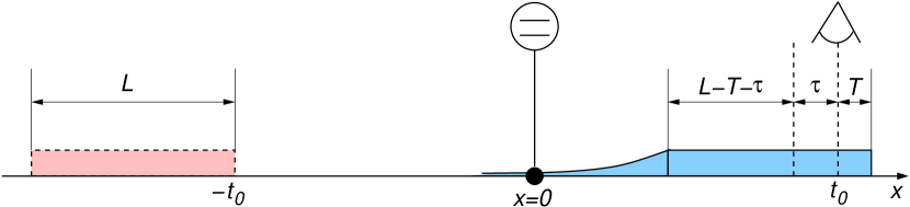
Figure 1: (Color online) Our system consists of a two-level emitter coupled to a waveguide (transmission line) at $x=0$. The sketch shows spatial snapshots of the wavepacket propagation. The coherent initial pulse $|\alpha_{0}\rangle$ of the length $L$ (shown in pink with dashed contour) is injected at time $t=-t_{0}$ and the point $x=-t_{0}$. At time $t=0$ its front hits the scatterer. The scattered pulse (shown in blue with solid contour) leaves the scattering region, and after time $t_{0}$ its front reaches a detector located at $x=t_{0}$. At time $t=t_{0}+T$ the detector starts counting photons which lasts during the time interval $\tau$. It is assumed that $t_{0}\gg L>\tau$.

I.2 Scattering approach, role of detector

In this paper we focus on a basic model consisting of a two-level qubit coupled to a 1D channel and driven by a coherent field. We develop a complete and exact quantum description of all physical properties of this system using the scattering formalism.

A characterization of different scattering regimes in this model can be obtained by introducing parameters quantifying (i) an initial state, (ii) a qubit (iii), a waveguide, and (iv) a detector. Throughout the paper we assume that the initial state is a pulse of the spatial length $L$. In the units $\hbar=v_{g}=1$, where $v_{g}$ is the group velocity of linearly dispersed photons in a waveguide, the parameter $1/L$ defines one of the important energy scales – the wavepacket width in the $k$-space. Another energy scale is given by the qubit relaxation rate $\Gamma=\pi g^{2}$, where $g$ is a photon-qubit interaction strength. In addition, we have a dimensionless parameter $\bar{N}$ characterizing the mean number of photons in the initial pulse. In terms of these parameters, one can distinguish three different regimes in this problem: (a) $\bar{N}\gg\Gamma L\gg 1$; (b) $\Gamma L\gg\bar{N}\gg 1$; (c) $\Gamma L\gg 1\gg\bar{N}$. Note that in all cases we assume $\Gamma L\gg 1$ meaning the long-$L$ (or narrow bandwidth) pulse’s limit.

The regime (a) was studied back in 1970’s in connection with the resonance fluorescence phenomenon Mollow (see also the review KM-rev ). In this regime, a semiclassical description of the laser beam is sufficient.

In contrast to the regime (a), in the regime (c) single-photon (elastic) processes dominate, while a contribution of many-photon (inelastic) processes to the scattering outcome is weak; the most remarkable inelastic effect in this regime is, perhaps, a formation of the two-photon bound state. Various aspects of the regime (c) have been recently studied in numerous publications cited above.

To complement the previous studies, we wish to achieve a comprehensive understanding of the crossover regime (b), where the mean number of scattered photons is already large, but the Rabi frequency $\propto\sqrt{\bar{N}\Gamma/L}$ is still much smaller than $\Gamma$. To this end, we apply the quantum scattering approach developed in our earlier paper PGnjp . It will be shown in the following that it is eventually capable to cover all three regimes, thereby establishing a theoretical platform for studying the classical-to-quantum crossover in this model.

In addition to the system related parameters, our approach can accommodate information contained in the detection protocol as shown in Fig. 1. A pulse of the spatial length $L$ (shown in pink) is injected into the waveguide at time $t=-t_{0}$ and the coordinate $x=-t_{0}$ (recall that $v_{g}=1$). Due to the linear dispersion, it moves without changing its shape toward the qubit coupled to the waveguide at the point $x=0$. From the time instant $t=0$ the photons in the pulse start interacting with the qubit, and this interaction lasts approximately for a time $\sim L$. Subsequently the scattered pulse leaves the interaction region around $x=0$ (only the transmitted part is shown in blue in the figure), its shape is being modified, and at $t=t_{0}$ its front reaches the detector (the “eye”) at the position $x=t_{0}$. To make the scattering formalism applicable we must assume that $t_{0}\gg L$, meaning that the detector is far away from the scattering region. After the front of the scattered pulse reaches the detector at $t=t_{0}$, the latter remains switched off during the waiting time $T$, and at $t=t_{0}+T$ it switches on and starts to count transmitted photons during the subsequent time interval $\tau$ (counting time). Thus, the setup in Fig. 1 is characterized by the two important time scales $T$ and $\tau$. In the following we will assume $L>\tau$ (which, in particular, allows us to take the limit $L\to\infty$ before the limit $\tau\to\infty$). This assumption is based on an instrumental possibility to create an initial wavepacket of a sufficiently narrow width in the $k$-space; from the conceptual viewpoint we impose this condition to enable an open-system description of the scattered pulse, for which the aforementioned order of limits is essential.

The detector-related time scales together with the system-related energy scales exhaust the most relevant parameters of this problem.

I.3 Physical observables and their generating function

Major statistical properties of a scattered light field are characterized by a collection of $m$-point ($m=2,4,\ldots$) correlation functions Glauber . Another basic observable quantity is a transmission (reflection) spectrum. It quantifies the amplitude of the transmitted (reflected) field, and it has been measured in various experiments with microwave transmission lines Astafiev , Dayan , coherent1 , coherent2 . A more involved quantity of interest is the resonance fluorescence power spectrum, which is a Fourier transform of the field-field ($g^{(1)}$) correlation function. This (Mollow) spectrum is know to feature a three-peak structure Mollow . Further experimental practice is to collect information about the density-density ($g^{(2)}$) correlation function using the Hanbury-Brown-Twiss setup HBT . Higher order correlators can also (at least, in principle) be accessed in an experiment, and this motivates us to study the generating function of all moments of the density operator, being related to the $m$-point functions. In mesoscopic physics, such a generating function is known as the Full Counting Statistics (FCS), though in the historical retrospective this concept has been originally introduced in the quantum-optical context Glauber , MaWo in order to characterize statistical properties of a non-interacting quantized electromagnetic field. Its fully quantum derivation has been presented in Ref. KK . For a coherent light field driving a two-level system (the resonance fluorescence model) the FCS has been studied in Mandel , Cook , Lenstra , Smirnov-Troshin . It has been observed Mandel that the FCS distribution of the fluorescent photons is narrower than the Poissonian distribution. An important measure of this effect is the Mandel’s $Q$-parameter, $Q=[\langle N^{(2)}\rangle-\langle N^{(1)}\rangle^{2}]/\langle N^{(1)}\rangle$ which is obtained from the first and the second factorial moments of the FCS.

Later on, the concept of the FCS has been borrowed and actively developed in the field of mesoscopic physics LL , LLL for studying statistical properties of electronic currents in meso- and nanoscopic devices for both non-interacting and interacting electrons NB , Belzig , BN , BUGS , GK , Schonh , KS , BSS , BBSS , CBS . It has been recently shown that the FCS can be very useful for characterizing classical-quantum crossover SB , quantum entanglement TF , KL , LeHur , and phase transitions IA , FG . The FCS of nonlocal observables can be used to quantify correlations GADP , IGD , Hoffer , LF , and prethermalization in many-body systems Kitagawa , prethermalization , as well as to define some kind of a topological order parameter IA2 .

The studies of the FCS in mesoscopic physics have generated a back flow of ideas to the quantum optics community. Inspired by the recent experiments in the context of the 1D resonance fluorescence, the subject of the FCS has received the renewed attention, see deflection , BB , Vogl , LJ .

I.4 This paper: content and results

Motivated by previous developments we revisit the original problem of computing the FCS for photons interacting with an emitter. This is the first goal of the present work. We give it a detailed quantum consideration, treating the interaction nonperturbatively. We present an exact calculation of the FCS in the basic model of light-matter interaction (see Fig. 1): a multimode propagating photonic field in 1D interacting with a two-level emitter. Since one of the objectives in nanophotonics research is to obtain strong photon nonlinearities as well as a strong photon-emitter interaction for the purpose of an efficient control over individual atoms and photons, knowledge of statistical properties of an interacting photon-emitter device becomes essential.

The geometry of our system (see Fig. 1) suggests to define the three types of the counting statistics: the FCS of transmitted photons, the FCS of reflected photons, and the FCS of the chiral model. Below we discuss this classification in more detail. The multimode nature of the waveguide implies an emergence of many-body correlations. As such, interactions modify the statistics of photons in forward and backward scattering channels in comparison with the Poissonian one of the incident coherent beam. As a by-product of our FCS computation, we revisit the transmission properties and evaluate the Mandel’s $Q$-factor exhibiting super-Poissonian, sub-Poissonian, and Poissonian statistics for the three counting models in question.

We also provide a new derivation of the Mollow spectrum based on knowledge of the exact scattering wavefunction that avoids the usage of the quantum regression theorem, and reproduces the original expression Mollow derived for the 3D scattering geometry. It helps to understand how the resonance fluorescence can be decomposed into elementary scattering processes.

Yet another quantity that has recently received a great deal of attention due to developments in quantum information science is the entanglement entropy, see, e.g., the recent review Eisert . While several measures of entanglement exist, the entropy of entanglement has several nice properties like additivity and convexity. In quantum information theory, the entanglement entropy gives the efficiency of conversion of partially entangled to maximally entangled states by local operations Bennett1 , Bennett2 . In other terms, it gives the amount of classical information required to specify the reduced density matrix. A large degree of entanglement is what makes quantum information exponentially more powerful than classical information, so states with lower entanglement entropy are less complex. For extended systems of condensed matter physics it is customary to distinguish between area and volume law Eisert behavior of the entanglement entropy. Here the notions of area or volume refer to a typical geometric measure of a region bounded by a subsystem $A$ with respect to the rest of a system. Thus in 1D case, relevant for our discussion here, the area of an interval $A$ consists of just two end points, while the volume is a length of the interval of the subsystem $A$. Systems with volume law behavior entanglement possess much higher potential for applications in quantum simulations and computing. It was shown Eisert that in most cases a quantum ground state wave function of gapped systems exhibits the area law, while typical excited states mostly follow the volume law. An intermediate logarithmic behavior of the entanglement entropy is related to gapless systems. These features should be understood as asymptotic properties of a system, when the area and the volume of a subsystem entangled with the rest part of a system become large. Our complete knowledge of the scattering state allows us to calculate explicitly the entanglement entropy of the scattered pulse’s interval of the length $\tau$ (see Fig. 1) for different values of $\tau$, $T$, and system parameters. The (dimensionless) duration $\Gamma\tau$ of the observation interval plays the role of the volume of the subsystem $A$ in this context. One of our central results in that section is a demonstration of the existence of the absolute limit for the entanglement entropy in our system: it is bounded by $\log 4$, the entropy of four-level system. Another important observation is that while the entanglement entropy at large $\tau$ asymptotically approaches the area law bounded by $\log 4$, it can behave very differently for small and intermediate values of $\tau$ – we even observe its nonmonotonous oscillatory behavior for some intermediate regime of parameters.

II Definitions and approximations

We start our analysis defining the model and approximations involved in its derivation, the bosonic operators creating the initial pulse, and the FCS.

II.1 Theoretical model.

II.1.1 Approximations and the effective Hamiltonian.

Our model is described by the Hamiltonian $H=H_{ph}+H_{em}+H_{ph-em}$, where $H_{ph}$ is the Hamiltonian of the free propagating photonic field, $H_{em}$ is the Hamiltonian of an emitter, and $H_{ph-em}$ describes the field-emitter coupling. We involve approximations which are customary in quantum optics: (i) the dipole approximation for the interacting Hamiltonian; (ii) the two-level approximation for the emitter Hamiltonian; (iii) the rotating wave approximation (RWA); and (iv) the Born-Markov approximation (energy independence) for the coupling constant. In addition, we linearize the photonic spectrum around some appropriately chosen frequency $\Omega_{0}$ which is commensurate with the emitter’s transition frequency $\Omega$, and extend the linearized dispersion to infinities. With these assumptions [except for (iii)] we obtain an effective low-energy Hamiltonian

$$H = \sum_{\xi=r,l}\int dk(\Omega_{0}+\xi k)a^{{\dagger}}_{\xi k}a_{\xi k}+\frac{\Omega}{2}\sigma^{z}$$ (1)

$$+ g_{0}\sum_{\xi=r,l}\int dk(a_{\xi k}^{{\dagger}}+a_{\xi k})(\sigma^{+}+\sigma^{-}),$$

featuring the two-branch linear dispersion with right- ($\xi=r=+$) and left- ($\xi=l=-$) propagating modes. Here $\sigma^{\pm}=(\sigma^{x}\pm i\sigma^{y})/2$ are expressed in terms of the Pauli matrices $\sigma^{a}$, $a=x,y,z$. The states of the emitter are separated by the transition frequency $\Omega$. To implement the RWA in a systematic way, we first perform the gauge transformation $H\to U^{{\dagger}}HU+i(dU^{{\dagger}}/dt)U$ with

$$U=\exp\left[-i\Omega_{0}t\left(\sum_{\xi=r,l}\int dk\,a^{{\dagger}}_{\xi k}a_{\xi k}+\frac{\sigma^{z}}{2}\right)\right],$$ (2)

which leads us to the Hamiltonian

$$H = \sum_{\xi=r,l}\int dk\,\xi\,k\,a^{{\dagger}}_{\xi k}a_{\xi k}+\frac{\Delta}{2}\sigma^{z}$$ (3)

$$+ g_{0}\sum_{\xi=r,l}\int dk(a_{\xi k}^{{\dagger}}\sigma^{-}+a_{\xi k}\sigma^{+})$$

$$+ g_{0}\sum_{\xi=r,l}\int dk(a_{\xi k}^{{\dagger}}\sigma^{+}e^{2i\Omega_{0}t}+a_{\xi k}\sigma^{-}e^{-2i\Omega_{0}t}),$$

where $\Delta=\Omega-\Omega_{0}$. As soon as $g_{0}^{2}/\Omega_{0}\ll 1$, the time-oscillating terms in (3) can be treated as a time-dependent perturbation. In zeroth order it is simply neglected, which is equivalent to the RWA. Note that this approximation is consistent with the assumption about the absence of lower and upper bounds in the linearized dispersion.

II.1.2 Transformation to the “even-odd” basis.

Due to energy independence of the coupling constant $g_{0}$, one can decouple the Hilbert space of the model defined in (3) into two sectors. To this end, one introduces even (symmetric) and odd (antisymmetric) combinations of fields corresponding to the same energy $|k|$

$$a_{ek}=\frac{a_{rk}+a_{l,-k}}{\sqrt{2}},\quad a_{ok}=\frac{a_{rk}-a_{l,-k}}{\sqrt{2}}.$$ (4)

By virtue of this canonical transformation the Hamiltonian (3) turns into a sum of the two terms, $H=H_{e}+H_{o}$, defined by

$$H_{e} = \int dk\left[k\,a^{\dagger}_{ek}a_{ek}+g\left(a^{\dagger}_{ek}\sigma^{-}+a_{ek}\sigma^{+}\right)\right]+\frac{\Delta}{2}\sigma^{z},$$

$$H_{o} = \int dk\,k\,a^{\dagger}_{ok}a_{ok},$$ (5)

where $g=g_{0}\sqrt{2}$. Note that the odd Hamiltonian $H_{o}$ is noninteracting, and therefore odd modes do not scatter off a local emitter ($S_{o}\equiv 1$). The even Hamiltonian $H_{e}$ can be interpreted in terms of a chiral model with a single branch of the linear dispersion.

A similar decomposition can be applied to an initial state. Both even and odd photons are labeled by a momentum value $k$ lying on a single branch of the linear dispersion.

II.2 Definitions of wave packet field operators and the initial state.

In order to define the incident coherent state we need field operators annihilating/creating states which are normalized by unity. The field operators $a_{k}$ and $a^{{\dagger}}_{k}$, which are the Fourier transforms of $a(x)$ and $a^{{\dagger}}(x)$, do not fulfill this requirement, as they obey the commutation relation $[a_{k},a^{\dagger}_{k^{\prime}}]=\delta(k-k^{\prime})$ (in other words, they annihilate and create unnormalizable states). To circumvent this difficulty, we construct wavepacket field operators

$$b_{k}^{\dagger} = \frac{1}{\sqrt{L}}\int_{-L/2}^{L/2}dxa^{\dagger}(x)e^{ikx},$$ (6)

which do satisfy the desired commutation relation $[b_{k},b_{k}^{\dagger}]=1$. For example, the operators $b_{r,k_{0}}^{\dagger}=\frac{1}{\sqrt{L}}\int_{-L/2}^{L/2}dxa^{\dagger}_{r}(x)e^{ik_{0}x}$ and $b_{l,-k_{0}}^{\dagger}=\frac{1}{\sqrt{L}}\int_{-L/2}^{L/2}dxa^{\dagger}_{l}(x)e^{-ik_{0}x}$ create wavepackets which are centered around $+k_{0}(-k_{0})$ of the right (left) branch of the spectrum and broadened over the width $\sim 2\pi/L$. In the coordinate representation, they create states which are spatially localized on a finite interval of the length $L$. We note the identity $[a_{\xi}(x),b_{\xi^{\prime},k_{0}}^{\dagger}]=\delta_{\xi\xi^{\prime}}\frac{e^{ik_{0}x}}{\sqrt{L}}\Theta(L/2-|x|)$. In the following, $k_{0}$ denotes the laser driving frequency (measured from the linearization point).

Having introduced $b_{r/l,k0}^{\dagger}$, we define the initial (incoming) state $|\mathrm{in}\rangle=|\alpha_{0}\rangle_{r}\otimes|\downarrow\rangle$, where the incident right-moving photons are prepared in the coherent state $|\alpha_{0}\rangle_{r}=D_{r}(\alpha_{0})|0\rangle$, and the two-level emitter is initially in the ground state $|\downarrow\rangle$. Here $|0\rangle$ denotes the photonic vacuum, and $D_{r}(\alpha_{0})=\exp(\alpha_{0}b^{\dagger}_{r,k_{0}}-\alpha_{0}^{*}b_{r,k_{0}})$ is the coherent state displacement operator.

The mean number of photons in the state $|\alpha_{0}\rangle_{r}$ is given by $\bar{N}_{0}=|\alpha_{0}|^{2}$. We also quote a useful relation

$$D_{r}^{\dagger}(\alpha_{0})a_{r}(x)D_{r}(\alpha_{0})=a_{r}(x)+\frac{\alpha_{0}e^{ik_{0}x}}{\sqrt{L}}\Theta(L/2-|x|),$$ (7)

which follows from the commutation relation between $a$ and $b^{\dagger}$ operators.

The initial coherent state defined in the original right-left basis admits a decomposition into the product state in the even-odd basis

$$|\alpha_{0}\rangle_{r} = e^{\alpha_{0}b^{{\dagger}}_{r,k_{0}}-|\alpha_{0}|^{2}/2}|0\rangle$$

$$= e^{(\alpha_{0}/\sqrt{2})b^{{\dagger}}_{e,k_{0}}-|\alpha_{0}|^{2}/4}e^{(\alpha_{0}/\sqrt{2})b^{{\dagger}}_{o,k_{0}}-|\alpha_{0}|^{2}/4}|0\rangle$$

$$\equiv D_{e}(\alpha)D_{o}(\alpha)|0\rangle\equiv|\alpha\rangle_{e}\otimes|\alpha\rangle_{o},$$

where $\alpha=\alpha_{0}/\sqrt{2}$, and the displacement operators $D_{e,o}$ are defined using the mutually commuting operators $b_{e,k_{0}}^{\dagger}$ and $b_{o,k_{0}}^{\dagger}$, respectively. Importantly, $\,{}_{r}\langle\alpha_{0}|\alpha_{0}\rangle_{r}=1$, i.e. the incoming state is properly normalized.

The major consequence of the even-odd decoupling is a factorization of the scattering operator $S$ into the product $S=S_{e}S_{o}$, where $S_{o}$ is the identity operator, and $S_{e}$ can be studied in the context of the effective one-channel chiral model described by $H_{e}$. Scattering in chiral models has been studied by us in Ref. PGnjp for arbitrary initial states, including the coherent state. In particular, we have established the explicit form of the operator $S_{e}$ in the latter case, which provides the full information about the scattering wavefunction. Here we take over this result and use it for calculation of observables announced in the Introduction. All expressions necessary for this purpose are quoted below for readers’ convenience.

II.3 Definition of the full counting statistics

The statistics of the initial field, defined by the probability $p_{\alpha_{0}}(n)$ to find $n$ photons in the mode $k_{0}$, is given by the Poissonian distribution $p_{\alpha_{0}}(n)=e^{-\bar{N}_{0}}\frac{\bar{N}_{0}^{n}}{n!}$ for the coherent field, with the mean value $\bar{N}_{0}=|\alpha_{0}|^{2}$. Due to the photonic dispersion and inelastic scattering processes photons can leak from the right-moving mode $k_{0}$ to other modes on both branches of the spectrum by virtue of scattering processes, thus modifying the photon statistics. A fraction of photons is reflected, and their statistics is also of great interest. We propose a calculation of the FCS in both forward and backward scattering channels, which is exact and nonperturbative in both $g_{0}$ and $\bar{N}_{0}$.

Generally speaking, the FCS can be defined as a generating function $F(\chi)=\sum_{n=0}^{\infty}e^{i\chi n}p(n)$ associated with a probability distribution $p(n)$ to detect $n$ photons in some given state. The function $F(\chi)$ generates $m$-th order moments of the distribution $p(n)$ which are determined by evaluating the $m$-th derivative with respect to $i\chi$ at $\chi=0$. The Fourier expansion of the $2\pi$-periodic function $F(\chi)$ yields power series in terms of the “fugacity” $z=e^{i\chi}$, $F(\chi)=\sum_{n=0}^{\infty}z^{n}p(n)\equiv{\hat{F}}(z)$. The normalization of a probability distribution implies $\hat{F}(1)=1$. The expansion $\hat{F}(z)=\sum_{r=0}^{\infty}\frac{(z-1)^{r}}{r!}\langle N^{(r)}\rangle$ around $z=1$ gives the factorial moments of a distribution $\langle N^{(r)}\rangle=\langle N(N-1)\ldots(N-r+1)\rangle$.

To define the photon FCS we need the two main constituents: (i) the scattering (outgoing) state $|\mathrm{out}\rangle=(S_{e}|\alpha\rangle_{e})\otimes|\alpha\rangle_{o}$ necessary to perform the average, and (ii) a meaningful and experimentally measurable counting operator $N$. In particular, as such we can choose the number of transmitted photons which pass through the detector during the time $\tau$ (see the Fig. 1). Because of the linear dispersion, the same operator characterizes the number of photons in the spatial interval of the length $v_{g}\tau$ viewed in the frame co-moving in the right direction with the velocity $v_{g}$. Introducing the coordinate system in this co-moving frame such that the pulse’s front has the coordinate value $+L/2$, we define the photon number operator

$$N_{r,\tau}=\int_{z_{1}}^{z_{2}}dxa_{r}^{\dagger}(x)a_{r}(x)$$ (8)

of transferred photons which appear in the spatial interval $[z_{1},z_{2}]$. Here $-L/2<z_{1}<z_{2}<L/2$ (we note that the tail of the scattered pulse extends to $-\infty$, see below; however, we will focus on counting intervals $\tau\equiv z_{2}-z_{1}<L$). The corresponding FCS reads

$$F_{r,\tau}(\chi_{0})=\langle e^{i\chi_{0}N_{r,\tau}}\rangle.$$ (9)

In the chosen coordinate system, the waiting time is expressed by $T=L/2-z_{2}$.

In the same setting one can consider the FCS of the chiral model.

To define the FCS for reflected photons, one can put the second detector at $x=-t_{0}$ and consider the co-moving frame with the velocity $-v_{g}$, defining in it the counting operator $N_{l,\tau}$ via $a_{l}(x)$.

III Method of computing observables based on exact scattering matrix

III.1 Scattering of the coherent state in the chiral model

As we discussed above, we need to know an expression $S_{e}|\alpha\rangle_{e}$ for the scattering state in the effective chiral model for the even modes. In this subsection we quote the result of Section 5 in Ref. PGnjp for the coherent light scattering in the chiral model. In particular, we copy the Eq. (134) from this reference, adapting notations therein to the present paper. The subscript $e$ is also omitted in the following.

Thus, for the incoming coherent state $|\alpha\rangle$ in the mode $k_{0}$, the outgoing scattering state amounts to $S_{0}|\alpha\rangle$, where

$$S_{0}=S_{0}^{a}[L/2,-L/2]+S_{0}^{b}[L/2,-L/2]\frac{\lambda}{\sqrt{2\Gamma}}A_{0}^{\dagger}.$$ (10)

The operator

$$A_{0}^{\dagger}=\sqrt{2\Gamma}\int_{-\infty}^{-L/2}dx_{0}e^{ik_{0}x_{0}}e^{-i(\delta+i\Gamma)(L/2+x_{0})}a^{\dagger}(x_{0}),$$ (11)

describing the states in the tail of the scattered pulse, is normalized by $\langle 0|A_{0}A_{0}^{\dagger}|0\rangle=1$.

In turn, the states within the initial pulse’s size $L$ are expressed via the operators

$$S_{0}^{a}[y,x] = 1+\sum_{n=1}^{\infty}\lambda^{n}\int{\cal D}x_{n}$$

$$\times d_{0}(y-x_{n})a^{\dagger}(x_{n})e^{ik_{0}x_{n}}$$

$$\times d_{0}(x_{n}-x_{n-1})a^{\dagger}(x_{n-1})e^{ik_{0}x_{n-1}}$$

$$\times \ldots d_{0}(x_{2}-x_{1})a^{\dagger}(x_{1})e^{ik_{0}x_{1}},$$

$$S_{0}^{b}[y,x] = d_{0}(y-x)+\sum_{n=1}^{\infty}\lambda^{n}\int{\cal D}x_{n}$$

$$\times d_{0}(y-x_{n})a^{\dagger}(x_{n})e^{ik_{0}x_{n}}$$

$$\times d_{0}(x_{n}-x_{n-1})a^{\dagger}(x_{n-1})e^{ik_{0}x_{n-1}}$$

$$\times \ldots d_{0}(x_{2}-x_{1})a^{\dagger}(x_{1})e^{ik_{0}x_{1}}d_{0}(x_{1}-x).$$

Here the parameter

$$\lambda=-\frac{2i\Gamma\alpha}{(\delta+i\Gamma)\sqrt{L}},$$ (14)

is expressed in terms of the detuning $\delta=k_{0}-\Delta$ and the relaxation rate $\Gamma=\pi g^{2}$; $d_{0}(x)=1-\exp[i(\delta+i\Gamma)x]$ is the bare single-photon propagator, and the short-hand notation has been used for the integration measure ${\cal D}x_{n}=\Theta(y>x_{n}>\ldots>x_{1}>x)dx_{n}\ldots dx_{1}$. We also consider $L/2\geq y>x\geq-L/2$.

For the later use we also define the following operators

$$S_{0}^{c}[y,x] = 1+\sum_{n=1}^{\infty}\lambda^{n}\int{\cal D}x_{n}$$

$$\times a^{\dagger}(x_{n})e^{ik_{0}x_{n}}d_{0}(x_{n}-x_{n-1})$$

$$\times a^{\dagger}(x_{n-1})e^{ik_{0}x_{n-1}}d_{0}(x_{n-1}-x_{n-2})\ldots$$

$$\times d_{0}(x_{2}-x_{1})a^{\dagger}(x_{1})e^{ik_{0}x_{1}},$$

$$S_{0}^{\bar{a}}[y,x] = 1+\sum_{n=1}^{\infty}\lambda^{n}\int{\cal D}x_{n}$$

$$\times a^{\dagger}(x_{n})e^{ik_{0}x_{n}}d_{0}(x_{n}-x_{n-1})$$

$$\times a^{\dagger}(x_{n-1})e^{ik_{0}x_{n-1}}d_{0}(x_{n-1}-x_{n-2})\ldots$$

$$\times a^{\dagger}(x_{1})e^{ik_{0}x_{1}}d_{0}(x_{1}-x).$$

The set of operators $S^{a}_{0},S^{b}_{0},S^{c}_{0},S^{\bar{a}}_{0}$ is complete in that sense that they exhaust all possible arrangements of the bare propagators $d_{0}(x)$.

III.2 Algebra of scattering operators

The scattering state (134) of Ref. PGnjp (equivalent of $S_{0}|\alpha\rangle$) can be used for a computation of observable quantities. In particular, we will be interested in correlation functions $\langle\alpha|S_{0}^{\dagger}a^{\dagger}(z_{1})\ldots a^{\dagger}(z_{m})a(z_{m})\ldots a(z_{1})S_{0}|\alpha\rangle$, and therefore we need to know how the local annihilation operators $a(z_{k})$ commute with the many-body scattering operator $S_{0}$ defined on a finite spatial interval. For a systematic treatment, we observe the following algebraic properties of the scattering operators $S^{a}_{0},S^{b}_{0},S^{c}_{0},S^{\bar{a}}_{0}$.

Let us choose an arbitrary point $z\in[x,y]$. Using the obvious identity

$$\Theta(y>x_{n}>\ldots>x_{1}>x)$$

$$= \sum_{j=0}^{n}\Theta(y>x_{n}>\!\ldots>\!x_{j+1}>z>x_{j}>\!\ldots>\!x_{1}>x),$$

where $x_{n+1}=y$ and $x_{0}=x$, one can show by rewriting Eqs. (III.1), (III.1), (III.1), and (III.1), that the operators $S^{a}_{0},S^{b}_{0},S^{c}_{0},S^{\bar{a}}_{0}$ satisfy the following closed algebra with respect to the interval splitting operation

$$S_{0}^{a}[y,x]\!=\!S_{0}^{a}[y,z]S_{0}^{a}[z,x]\!+S_{0}^{b}[y,z]\!\{S_{0}^{c}[z,x]\!-\!S_{0}^{a}[z,x]\},$$

$$S_{0}^{b}[y,x]\!=\!S_{0}^{a}[y,z]S_{0}^{b}[z,x]\!+S_{0}^{b}[y,z]\!\{S_{0}^{\bar{a}}[z,x]\!-\!S_{0}^{b}[z,x]\},$$

$$S_{0}^{c}[y,x]\!=\!S_{0}^{c}[y,z]S_{0}^{a}[z,x]\!+S_{0}^{\bar{a}}[y,z]\!\{S_{0}^{c}[z,x]\!-\!S_{0}^{a}[z,x]\},$$

$$S_{0}^{\bar{a}}[y,x]\!=\!S_{0}^{c}[y,z]S_{0}^{b}[z,x]\!+S_{0}^{\bar{a}}[y,z]\!\{S^{\bar{a}}[z,x]\!-\!S_{0}^{b}[z,x]\}.$$

(18)

If one divides the interval $[x,y]$ into three parts $y>z_{2}>z_{1}>x$ by arbitrary points $z_{1}$ and $z_{2}$, one can prove by a direct calculation that the algebra (18) is associative, as expected.

The algebra (18) also allows us to express the action of annihilation operators on the scattered state in a simple form

$$a(z)S_{0}^{a}[y,x]|0\rangle=S_{0}^{b}[y,z]\lambda e^{ik_{0}z}S_{0}^{a}[z,x]|0\rangle,$$ (19)

$$a(z)S_{0}^{b}[y,x]|0\rangle=S_{0}^{b}[y,z]\lambda e^{ik_{0}z}S_{0}^{b}[z,x]|0\rangle,$$ (20)

$$a(z)S_{0}^{c}[y,x]|0\rangle=S_{0}^{\bar{a}}[y,z]\lambda e^{ik_{0}z}S_{0}^{a}[z,x]|0\rangle,$$ (21)

$$a(z)S_{0}^{\bar{a}}[y,x]|0\rangle=S_{0}^{\bar{a}}[y,z]\lambda e^{ik_{0}z}S_{0}^{b}[z,x]|0\rangle.$$ (22)

For the proof of (19)-(22) we used the property $d_{0}(0)=0$.

Similarly, for an action of the ordered product of two annihilation operators $a(z_{2})a(z_{1})$, with $y>z_{2}>z_{1}>x$, we obtain

$$a(z_{2})a(z_{1})S_{0}^{a}[y,x]|0\rangle$$

$$= S_{0}^{b}[y,z_{2}]\lambda e^{ik_{0}z_{2}}S_{0}^{b}[z_{2},z_{1}]\lambda e^{ik_{0}z_{1}}S_{0}^{a}[z_{1},x]|0\rangle,$$

$$a(z_{2})a(z_{1})S_{0}^{b}[y,x]|0\rangle$$

$$= S_{0}^{b}[y,z_{2}]\lambda e^{ik_{0}z_{2}}S_{0}^{b}[z_{2},z_{1}]\lambda e^{ik_{0}z_{1}}S_{0}^{b}[z_{1},x]|0\rangle,$$

$$a(z_{2})a(z_{1})S_{0}^{c}[y,x]|0\rangle$$

$$= S_{0}^{\bar{a}}[y,z_{2}]\lambda e^{ik_{0}z_{2}}S_{0}^{b}[z_{2},z_{1}]\lambda e^{ik_{0}z_{1}}S_{0}^{a}[z_{1},x]|0\rangle,$$

$$a(z_{2})a(z_{1})S_{0}^{\bar{a}}[y,x]|0\rangle$$

$$= S_{0}^{\bar{a}}[y,z_{2}]\lambda e^{ik_{0}z_{2}}S_{0}^{b}[z_{2},z_{1}]\lambda e^{ik_{0}z_{1}}S_{0}^{b}[z_{1},x]|0\rangle.$$

Iterating this procedure, one can find an action of the ordered product of $m$ annihilation operators $a(z_{m})\ldots a(z_{1})$, $y>z_{m}>\ldots z_{1}>x$. It produces the product of $m+1$ $S$-operators, what can be symbolically written as

$$a^{m}S_{0}^{a} \to S_{0}^{b}\ldots S_{0}^{b}\ldots S_{0}^{a},$$ (27)

$$a^{m}S_{0}^{b} \to S_{0}^{b}\ldots S_{0}^{b}\ldots S_{0}^{b},$$ (28)

$$a^{m}S_{0}^{c} \to S_{0}^{\bar{a}}\ldots S_{0}^{b}\ldots S_{0}^{a},$$ (29)

$$a^{m}S_{0}^{\bar{a}} \to S_{0}^{\bar{a}}\ldots S_{0}^{b}\ldots S_{0}^{b}.$$ (30)

Note that in all intermediate positions appears only $S_{0}^{b}$. To classify leftmost and rightmost operators in these expressions, we introduce the mappings $\sigma$ and $\mu$ according to the table

$$\sigma(a)= \!b,\quad\mu(a)= \!a,$$ (31)

$$\sigma(b)= \!b,\quad\mu(b)= \!b,$$ (32)

$$\sigma(c)= \!\bar{a},\quad\mu(c)= \!a,$$ (33)

$$\sigma(\bar{a})= \!\bar{a},\quad\mu(\bar{a})= \!b.$$ (34)

In their terms, the relations (27)-(30) acquire the compact form

$$a^{m}S_{0}^{\beta}\to S_{0}^{\sigma(\beta)}\left(S_{0}^{b}\right)^{m-1}S_{0}^{\mu(\beta)}.$$ (35)

III.3 Dressing $S$-operators

In the following we will also need shifted scattering operators

$$S_{v}^{\beta}[y,x] = D^{\dagger}(v)S_{0}^{\beta}[y,x]D(v)$$ (36)

$$= e^{v^{*}b_{k_{0}}}S^{\beta}[y,x]e^{-v^{*}b_{k_{0}}},$$

where $\beta=a,b,c,\bar{a}$, and $D(v)=\exp[vb_{k_{0}}^{\dagger}-v^{*}b_{k_{0}}]$ is the displacement operator of the fields, such that $D^{\dagger}(v)a^{\dagger}(x)D(v)=a^{\dagger}(x)+v^{*}e^{-ik_{0}x}/\sqrt{L}$. Our next goal is to establish explicit expressions for the operators $S_{v}^{\beta}[y,x]$ for arbitrary complex-valued parameter $v$.

Performing the displacement (36), we obtain the new series in field operators defining $S_{v}^{a,b,c,\bar{a}}$. Appropriately reorganizing (re-summing) them, we find the following expressions

$$S_{v}^{a}[y,x] = \tilde{d}_{v}(y-x)+\sum_{n=1}^{\infty}\lambda^{n}\int{\cal D}x_{n}$$

$$\times d_{v}(y-x_{n})a^{\dagger}(x_{n})e^{ik_{0}x_{n}}$$

$$\times d_{v}(x_{n}-x_{n-1})a^{\dagger}(x_{n-1})e^{ik_{0}x_{n-1}}$$

$$\times \ldots d_{v}(x_{2}-x_{1})a^{\dagger}(x_{1})e^{ik_{0}x_{1}}\tilde{d}_{v}(x_{1}-x),$$

$$S_{v}^{b}[y,x] = d_{v}(y-x)+\sum_{n=1}^{\infty}\lambda^{n}\int{\cal D}x_{n}$$

$$\times d_{v}(y-x_{n})a^{\dagger}(x_{n})e^{ik_{0}x_{n}}$$

$$\times d_{v}(x_{n}-x_{n-1})a^{\dagger}(x_{n-1})e^{ik_{0}x_{n-1}}$$

$$\times \ldots d_{v}(x_{2}-x_{1})a^{\dagger}(x_{1})e^{ik_{0}x_{1}}d_{v}(x_{1}-x),$$

$$S_{v}^{c}[y,x] = \tilde{\tilde{d}}_{v}(y-x)+\sum_{n=1}^{\infty}\lambda^{n}\int{\cal D}x_{n}$$

$$\times \tilde{d}_{v}(y-x_{n})a^{\dagger}(x_{n})e^{ik_{0}x_{n}}$$

$$\times d_{v}(x_{n}-x_{n-1})a^{\dagger}(x_{n-1})e^{ik_{0}x_{n-1}}$$

$$\times \ldots d_{v}(x_{2}-x_{1})a^{\dagger}(x_{1})e^{ik_{0}x_{1}}\tilde{d}_{v}(x_{1}-x),$$

$$S_{v}^{\bar{a}}[y,x] = \tilde{d}_{v}(y-x)+\sum_{n=1}^{\infty}\lambda^{n}\int{\cal D}x_{n}$$

$$\times \tilde{d}_{v}(y-x_{n})a^{\dagger}(x_{n})e^{ik_{0}x_{n}}$$

$$\times d_{v}(x_{n}-x_{n-1})a^{\dagger}(x_{n-1})e^{ik_{0}x_{n-1}}$$

$$\times \ldots d_{v}(x_{2}-x_{1})a^{\dagger}(x_{1})e^{ik_{0}x_{1}}d_{v}(x_{1}-x),$$

as well as

$$S_{v} = D^{\dagger}(v)S_{0}D(v)$$ (41)

$$= S_{v}^{a}[L/2,-L/2]+S^{b}_{v}[L/2,-L/2]\frac{\lambda}{\sqrt{2\Gamma}}A_{0}^{\dagger},$$

where

$$d_{v}(x) = -\frac{p_{+}+p_{-}}{p_{+}-p_{-}}\left[e^{-ip_{+}x}-e^{-ip_{-}x}\right],$$ (42)

$$\tilde{d}_{v}(x) = -\frac{p_{-}}{p_{+}-p_{-}}e^{-ip_{+}x}+\frac{p_{+}}{p_{+}-p_{-}}e^{-ip_{-}x},$$ (43)

$$\tilde{\tilde{d}}_{v}(x) = -\frac{p_{-}^{2}}{p_{+}^{2}-p_{-}^{2}}e^{-ip_{+}x}+\frac{p_{+}^{2}}{p_{+}^{2}-p_{-}^{2}}e^{-ip_{-}x}$$ (44)

$$\equiv \tilde{d}_{v}(x)+\frac{i\lambda v^{*}}{(\delta+i\Gamma)\sqrt{L}}d_{v}(x)$$

are the dressed single-photon propagators, and $p_{\pm}\equiv p_{\pm}(v^{*})=\frac{-(\delta+i\Gamma)\pm\sqrt{(\delta+i\Gamma)^{2}+8\Gamma\alpha v^{*}/L}}{2}$.

Additional details on evaluation of (III.3)-(III.3) are presented in the Appendix A.

III.4 Factorization property

To evaluate the FCS we prove the following key property of generalized $m$-point correlation functions: their factorization into the $(m+1)$-fold product of the two-point functions.

Generalized correlation functions are defined by

$$G_{\beta^{\prime}\beta}^{(m)}(\{z_{l}\};y,x)$$

$$= \langle 0|S_{u}^{\beta^{\prime}\,\dagger}[y,x]\left(:\prod_{l=1}^{m}a^{\dagger}(z_{l})a(z_{l}):\right)S_{v}^{\beta}[y,x]|0\rangle,$$

where the “time-forward” $S_{v}^{\beta}$ and the “time-backward” $S_{u}^{\beta^{\prime}\,\dagger}$ scattering operators depend on different and arbitrary displacement parameters $v$ and $u$, respectively. We also assume here that $y>z_{m}>\ldots>z_{1}>x$. Note that an additional symbol for the path-ordering in this expression is not required: operators $a(z_{l})$ and $a(z_{l^{\prime}})$ commute with each other, since (i) they are bosonic, and (ii) they are written in the interaction picture (which is equivalent to the Schrödinger picture in the co-moving frame).

We observe that the relations (18) are also fulfilled by the dressed operators $S_{v}^{\beta}$: one has just to dress (18) with $D(v)$. Along with the property $d_{v}(0)=0$, this implies that all relations (19)-(35) also remain valid under the replacement $S_{0}^{\beta}\to S_{v}^{\beta}$. These properties allow us to split both $S_{v}^{\beta}$ and $S_{u}^{\beta^{\prime}\,\dagger}$ into $m+1$ operators defined on the ordered intervals, see Eq. (35). Applying the Wick’s theorem, we contract operators from $S_{v}^{\beta}$ and $S_{u}^{\beta^{\prime}\,\dagger}$ belonging to the same interval; in total we have $m+1$ pairwise contractions of intervals. This procedure leads to a factorization of (III.4)

$$G_{\beta^{\prime}\beta}^{(m)}(\{z_{l}\};y,x)=|\lambda|^{2m}\mathcal{G}_{\sigma(\beta^{\prime})\sigma(\beta)}(y-z_{m})$$

$$\qquad\times\left[\prod_{l=1}^{m-1}\mathcal{G}_{bb}(z_{l+1}-z_{l})\right]\mathcal{G}_{\mu(\beta^{\prime})\mu(\beta)}(z_{1}-x)$$ (46)

into the product of $m+1$ two-point functions defined by

$$\mathcal{G}_{\beta^{\prime}\beta}(z_{l+1}-z_{l}) = \langle 0|S_{u}^{\beta^{\prime}\,\dagger}[z_{l+1},z_{l}]S_{v}^{\beta}[z_{l+1},z_{l}]|0\rangle.$$ (47)

In the following we will also use the special case of (47) with $u=v=\alpha$

$$\bar{\mathcal{G}}_{\beta^{\prime}\beta}(z_{l+1}-z_{l}) = \langle 0|S_{\alpha}^{\beta^{\prime}\,\dagger}[z_{l+1},z_{l}]S_{\alpha}^{\beta}[z_{l+1},z_{l}]|0\rangle,$$ (48)

corresponding to the standard definition of the correlation functions. The factorization property (46) in this case is well-known (see, e.g., Ref. MaWo ).

IV Computation of the FCS

IV.1 Detailing the definition

In our setup shown in Fig. 1 we have the right-moving photons in the incoming state. Therefore, in the outgoing state the right-moving photons correspond to the transmitted particles, while the left-moving photons are those which are reflected. Extending the definition (9) we represent

$$F_{r/l,\tau}(\chi_{0}) = \langle 0|D_{o}^{\dagger}(\alpha)D_{e}^{\dagger}(\alpha)S_{0}^{(e)\,\dagger}$$ (49)

$$\times e^{i\chi_{0}N_{r/l,\tau}}S_{0}^{(e)}D_{e}(\alpha)D_{o}(\alpha)|0\rangle,$$

where

$$N_{r/l,\tau}=\int_{z_{1}}^{z_{2}}dx\frac{a_{e}^{\dagger}(x)\pm a_{o}^{\dagger}(x)}{\sqrt{2}}\frac{a_{e}(x)\pm a_{o}(x)}{\sqrt{2}}.$$ (50)

Since $D_{o}(\alpha)$ commutes with $D_{e}(\alpha)$ and $S_{0}^{(e)}$, and it holds

$$D_{o}(\alpha)^{\dagger}N_{r/l,\tau}D_{o}(\alpha)=D_{e}(\pm\alpha)^{\dagger}N_{r/l,\tau}D_{e}(\pm\alpha),$$ (51)

we can cast (49) to

$$F_{r/l,\tau}(\chi) = \langle 0|D_{e}^{\dagger}(\alpha)S_{0}^{(e)\,\dagger}D_{e}^{\dagger}(\pm\alpha)$$ (52)

$$\times e^{i\chi_{0}N_{r/l,\tau}}D_{e}(\pm\alpha)S_{0}^{(e)}D_{e}(\alpha)|0\rangle.$$

Using the identity

$$e^{i\chi_{0}N_{r/l,\tau}}=:e^{(z_{0}-1)N_{r/l,\tau}}:$$

$$= 1+\sum_{m=1}^{\infty}(z_{0}-1)^{m}\int{\cal D}z^{\prime}_{m}\left(:\prod_{k=1}^{m}a_{r/l}^{\dagger}(z^{\prime}_{k})a_{r/l}(z^{\prime}_{k}):\right),$$

where $z_{0}=e^{i\chi_{0}}$, and taking into account that in (52) there are only even operators from both sides of $e^{i\chi_{0}N_{r/l,\tau}}$ as well as the vacuum average is performed, we can integrate out the odd modes. It can be effectively done by replacing $a_{r/l}^{\dagger}(z^{\prime}_{k})\to\frac{a_{e}^{\dagger}(z^{\prime}_{k})}{\sqrt{2}}$ and $a_{r/l}(z^{\prime}_{k})\to\frac{a_{e}(z^{\prime}_{k})}{\sqrt{2}}$ in (IV.1). This eventually results in the replacement

$$e^{i\chi_{0}N_{r/l,\tau}}\to e^{i\chi N_{e,\tau}},$$ (54)

where

$$N_{e,\tau}=\int_{z_{1}}^{z_{2}}dxa_{e}^{\dagger}(x)a_{e}(x),$$ (55)

and $\chi$ is defined by $z-1=\frac{z_{0}-1}{2}$ and $z=e^{i\chi}$. Thus,

$$F_{r/l,\tau}(\chi) = \langle 0|D_{e}^{\dagger}(\alpha)S_{0}^{(e)\,\dagger}D_{e}^{\dagger}(\pm\alpha)$$ (56)

$$\times e^{i\chi N_{e,\tau}}D_{e}(\pm\alpha)S_{0}^{(e)}D_{e}(\alpha)|0\rangle.$$

For the chiral model, we define the FCS by

$$F_{e,\tau}(\chi)=\langle 0|D_{e}^{\dagger}(\alpha)S_{0}^{(e)\,\dagger}e^{i\chi N_{e,\tau}}S_{0}^{(e)}D_{e}(\alpha)|0\rangle.$$ (57)

This expression is very similar to (56), so we can combine them together

$$F_{\tau}^{(\kappa)}(\chi) = \langle 0|D^{\dagger}(\alpha)S_{0}^{\dagger}D^{\dagger}((\kappa-1)\alpha)$$ (58)

$$\times e^{i\chi N_{\tau}}D((\kappa-1)\alpha)S_{0}D(\alpha)|0\rangle,$$

where the parameter $\kappa=0,1,2$ distinguishes between the reflected, chiral, and transmitted modes, respectively. We have also suppressed the label $e$, since all subsequent calculations will be performed in the effective chiral basis using the results of the previous section.

After a simple transformation of (58) we find

$$F_{\tau}^{(\kappa)}(\chi) = e^{-\kappa^{2}|\alpha|^{2}}\langle 0|S_{0}^{\dagger}e^{-(\kappa-1)\alpha b_{k_{0}}^{\dagger}}e^{\kappa\alpha^{*}b_{k_{0}}}$$ (59)

$$\times e^{i\chi N_{\tau}}e^{\kappa\alpha b_{k_{0}}^{\dagger}}e^{-(\kappa-1)\alpha^{*}b_{k_{0}}}S_{0}|0\rangle,$$

which is our starting expression for a computation of the FCS.

IV.2 Integrating out the “future” and the “past”

The operator $N_{\tau}=\int_{z_{1}}^{z_{2}}dxa^{\dagger}(x)a(x)$ in the definition (59) contains only fields belonging to the counting interval $[z_{1},z_{2}]$. In turn, the operator

$$b_{k_{0}}=\frac{1}{\sqrt{L}}\int_{-L/2}^{L/2}dx\,a(x)\,e^{-ik_{0}x}=\bar{b}_{k_{0}}+\tilde{b}_{k_{0}}$$ (60)

contains the counting part

$$\bar{b}_{k_{0}} = \frac{1}{\sqrt{L}}\int_{z_{1}}^{z_{2}}dx\,a(x)\,e^{-ik_{0}x},$$ (61)

and its complement $\tilde{b}_{k_{0}}=b_{k_{0}}^{f}+b_{k_{0}}^{p}$. The latter consists of the “future” ($z_{1}>x>-L/2$) and “past” ($L/2>x>z_{2}$) parts, see Fig. 1, which are defined by

$$b^{f}_{k_{0}} = \frac{1}{\sqrt{L}}\int_{-L/2}^{z_{1}}dx\,a(x)\,e^{-ik_{0}x},$$ (62)

$$b^{p}_{k_{0}} = \frac{1}{\sqrt{L}}\int_{z_{2}}^{L/2}dx\,a(x)\,e^{-ik_{0}x}.$$ (63)

Integrating out the states lying outside of the counting interval (see the Appendix B), we obtain

$$F_{\tau}^{(\kappa)}(\chi)e^{-(z-1)\kappa^{2}|\alpha|^{2}\frac{\tau}{L}}$$ (64)

$$= \left[1+R(T)\left(1-\frac{|\lambda|^{2}}{2\Gamma}\right)-2\,\mathrm{Re}\,C(T)\right]$$

$$\times\left(\Lambda_{aa}(\tau)+\frac{|\lambda|^{2}}{2\Gamma}\Lambda_{bb}(\tau)\right)$$

$$+ R(T)\left(\Lambda_{cc}(\tau)+\frac{|\lambda|^{2}}{2\Gamma}\Lambda_{\bar{a}\bar{a}}(\tau)\right)$$

$$+ [C(T)-R(T)]\left(\Lambda_{ac}(\tau)+\frac{|\lambda|^{2}}{2\Gamma}\Lambda_{b\bar{a}}(\tau)\right)$$

$$+ [C^{*}(T)-R(T)]\left(\Lambda_{ca}(\tau)+\frac{|\lambda|^{2}}{2\Gamma}\Lambda_{\bar{a}b}(\tau)\right),$$

where

$$\Lambda_{\beta^{\prime}\beta}(\tau)=\langle 0|S_{u}^{\beta^{\prime}\,\dagger}[z_{2},z_{1}]e^{i\chi N_{\tau}}S_{v}^{\beta}[z_{2},z_{1}]|0\rangle$$ (65)

evaluated at $u=z_{\kappa}\alpha$ and $v^{*}=z_{\kappa}\alpha^{*}$, where $z_{\kappa}=\kappa(z-1)+1$, and

$$R(T) = \bar{\mathcal{G}}_{bb}(L/2-z_{2}),$$ (66)

$$C(T) = \bar{\mathcal{G}}_{ab}(L/2-z_{2}).$$ (67)

The properties of the functions $R(T)$ and $C(T)$ are summarized in the Appendix E.

The last remaining step is to compute the terms (65). Using the identity

$$e^{i\chi N_{\tau}}=:e^{(z-1)N_{\tau}}:$$ (68)

$$=1+\sum_{m=1}^{\infty}(z-1)^{m}\int{\cal D}z^{\prime}_{m}\left(:\prod_{l=1}^{m}a^{\dagger}(z^{\prime}_{l})a(z^{\prime}_{l}):\right),$$

the definition of the generalized correlation functions (III.4), and their factorization property (46), we express

$$\Lambda_{\beta^{\prime}\beta}(\tau)=\mathcal{G}_{\beta^{\prime}\beta}(z_{2}-z_{1})+\sum_{m=1}^{\infty}\left[(z-1)|\lambda|^{2}\right]^{m}$$

$$\qquad\times\int{\cal D}z^{\prime}_{m}\mathcal{G}_{\sigma(\beta^{\prime})\sigma(\beta)}(z_{2}-z^{\prime}_{m})$$

$$\qquad\times\left[\prod_{l=1}^{m-1}\mathcal{G}_{bb}(z^{\prime}_{l+1}-z^{\prime}_{l})\right]\mathcal{G}_{\mu(\beta^{\prime})\mu(\beta)}(z^{\prime}_{1}-z_{1}).$$ (69)

Defining the Laplace transform for $x>0$ and its inverse

$$\mathcal{G}_{\beta^{\prime}\beta}(p) = \int_{0}^{\infty}dx\,\mathcal{G}_{\beta^{\prime}\beta}(x)e^{ipx},$$ (70)

$$\mathcal{G}_{\beta^{\prime}\beta}(x) = \int_{-\infty+i0}^{\infty+i0}\frac{dp}{2\pi}e^{-ipx}\mathcal{G}_{\beta^{\prime}\beta}(p),$$ (71)

we establish

$$\Lambda_{\beta^{\prime}\beta}(\tau)=\int\frac{dp}{2\pi}e^{-ip\tau}\left[\mathcal{G}_{\beta^{\prime}\beta}(p)\right.$$

$$\left.+(z-1)|\lambda|^{2}\frac{\mathcal{G}_{\sigma(\beta^{\prime})\sigma(\beta)}(p)\mathcal{G}_{\mu(\beta^{\prime})\mu(\beta)}(p)}{1-(z-1)|\lambda|^{2}\mathcal{G}_{bb}(p)}\right].$$ (72)

The Laplace transforms (70) for all components $\mathcal{G}_{\beta^{\prime}\beta}(p)$ are listed in the Appendix C. With their help we find (see the Appendix D) the following expressions

$$\Lambda_{aa}(\tau)+\frac{|\lambda|^{2}}{2\Gamma}\Lambda_{bb}(\tau)$$

$$= \int\frac{dp}{2\pi}\frac{ie^{-ip\tau}}{p+\frac{\Omega_{r}^{2}}{R_{0}(p)}(z-1)(p+i\Gamma)[i\Gamma-\kappa(p+i\Gamma)]}$$

$$\times\left[1-\frac{\Omega_{r}^{2}\kappa(z-1)(p+i\Gamma)}{2R_{0}(p)}\right],$$

$$\Lambda_{cc}(\tau)+\frac{|\lambda|^{2}}{2\Gamma}\Lambda_{\bar{a}\bar{a}}(\tau)$$

$$= \int\frac{dp}{2\pi}\frac{ie^{-ip\tau}}{p+\frac{\Omega_{r}^{2}}{R_{0}(p)}(z-1)(p+i\Gamma)[i\Gamma-\kappa(p+i\Gamma)]}$$

$$\times\left[1+\frac{|\lambda|^{2}}{2\Gamma}+\frac{i\Gamma\Omega_{r}^{2}(z-1)(1-\kappa)}{2R_{0}(p)}\left(1+\frac{(p+2i\Gamma)^{2}}{\delta^{2}+\Gamma^{2}}\right)\right.$$

$$\left.-\frac{\Omega^{2}_{r}\kappa(z-1)(p+i\Gamma)}{R_{0}(p)}\left(1+\frac{\Omega_{r}^{2}(\kappa(z-1)+3)}{8(\delta^{2}+\Gamma^{2})}\right)\right],$$

$$\Lambda_{ca}(\tau)+\frac{|\lambda|^{2}}{2\Gamma}\Lambda_{\bar{a}b}(\tau)$$

$$= \int\frac{dp}{2\pi}\frac{ie^{-ip\tau}}{p+\frac{\Omega_{r}^{2}}{R_{0}(p)}(z-1)(p+i\Gamma)[i\Gamma-\kappa(p+i\Gamma)]}$$

$$\times\left[1+\frac{i\Gamma\Omega_{r}^{2}(z-1)(1-\kappa)(p+\delta+i\Gamma)}{2R_{0}(p)(\delta-i\Gamma)}\right.$$

$$\left.\quad-\frac{\Omega_{r}^{2}\kappa(z-1)(p+i\Gamma)}{2R_{0}(p)}\left(1+\frac{p(p+\delta+i\Gamma)}{2(p+i\Gamma)(\delta-i\Gamma)}\right)\right],$$

where $\Omega_{r}=\sqrt{8\Gamma|\alpha|^{2}/L}$ denotes the Rabi frequency (note also the relation $\frac{|\lambda|^{2}}{2\Gamma}=\frac{\Omega_{r}^{2}}{4(\delta^{2}+\Gamma^{2})}$), and

$$R_{0}(p) = p^{3}+4i\Gamma p^{2}-p\left(\Omega_{r}^{2}+\delta^{2}+5\Gamma^{2}\right)$$ (76)

$$-i\Gamma\left(\Omega_{r}^{2}+2\delta^{2}+2\Gamma^{2}\right)$$

is the third-order polynomial. An expression for $\Lambda_{ac}(\tau)+\frac{|\lambda|^{2}}{2\Gamma}\Lambda_{b\bar{a}}(\tau)$ is obtained from (IV.2) by flipping the sign $\delta\to-\delta$.

The expressions (64) and (IV.2)-(76) completely define the FCS for reflected, chiral, and transmitted photons in the model under consideration. One should also keep in mind that for $\kappa=0,2$ it is necessary to replace in the end of calculation $z-1\to\frac{z_{0}-1}{2}$, since the counting parameter for the reflected and transmitted photons is $\chi_{0}$, and it is related to $z_{0}=e^{i\chi_{0}}$ (see also discussion before (56)).

IV.3 Normalization of probability distribution

We must check normalization of the probability distribution generated by (64), which is expressed by the condition $F_{\tau}^{(\kappa)}(0)=1$. Noticing that at $\chi=0$ the functions $\Lambda_{\beta^{\prime}\beta}(\tau)$, $\mathcal{G}_{\beta^{\prime}\beta}(\tau)$, and $\bar{\mathcal{G}}_{\beta^{\prime}\beta}(\tau)$ coincide with each other, we check the following identities

$$\bar{\mathcal{G}}_{aa}(\tau)+\frac{|\lambda|^{2}}{2\Gamma}\bar{\mathcal{G}}_{bb}(\tau) = 1,$$ (77)

$$\bar{\mathcal{G}}_{cc}(\tau)+\frac{|\lambda|^{2}}{2\Gamma}\bar{\mathcal{G}}_{\bar{a}\bar{a}}(\tau) = 1+\frac{|\lambda|^{2}}{2\Gamma},$$ (78)

$$\bar{\mathcal{G}}_{ca}(\tau)+\frac{|\lambda|^{2}}{2\Gamma}\bar{\mathcal{G}}_{\bar{a}b}(\tau) = 1,$$ (79)

which hold for arbitrary $\tau$, by setting $z=1$ in (IV.2)-(IV.2), and insert them into (64). We see that $F_{\tau}^{(\kappa)}(0)=1$ is indeed fulfilled for all $\tau$ and $T$. This also means that the scattering wavefunction is properly normalized.

IV.4 Limiting cases of the waiting time $T$

IV.4.1 Waiting regime $T\to\infty$

One of the important detection regimes is when the detector’s waiting time is long enough, $T\to\infty$, what physically means that $T$ is much larger than all system’s time scales, but still smaller than $L$. Depending on the context we will also call this regime stationary (for the resonance fluorescence) and bulk (for the entanglement entropy, see below).

The stationary values $R(\infty)=C(\infty)=\frac{\Gamma}{\Gamma+|\lambda|^{2}}$ (see the Appendix E) allow us to express (64) as

$$F_{\tau}^{(\kappa)}(\chi)e^{-(z-1)\kappa^{2}|\alpha|^{2}\frac{\tau}{L}}$$

$$= \frac{|\lambda|^{2}}{2(\Gamma+|\lambda|^{2})}\left(\Lambda_{aa}(\tau)+\frac{|\lambda|^{2}}{2\Gamma}\Lambda_{bb}(\tau)\right)$$

$$+\frac{\Gamma}{\Gamma+|\lambda|^{2}}\left(\Lambda_{cc}(\tau)+\frac{|\lambda|^{2}}{2\Gamma}\Lambda_{\bar{a}\bar{a}}(\tau)\right)$$

$$= \int\frac{dp}{2\pi}\frac{ie^{-ip\tau}W^{(\kappa)}(p)}{p+\frac{\Omega_{r}^{2}}{R_{0}(p)}(z-1)(p+i\Gamma)[i\Gamma-\kappa(p+i\Gamma)]},$$

where

$$W^{(\kappa)}(p) = 1+\frac{\Gamma\Omega_{r}^{2}(z-1)}{(|\lambda|^{2}+\Gamma)R_{0}(p)}$$

$$\times \left[\frac{i\Gamma(1-\kappa)}{2}\left(1+\frac{(p+2i\Gamma)^{2}}{\delta^{2}+\Gamma^{2}}\right)\right.$$

$$- \left.\kappa(p+i\Gamma)\left(1+\frac{\Omega_{r}^{2}(\kappa(z-1)+4)}{8(\delta^{2}+\Gamma^{2})}\right)\right].$$

To find the relation of this result to the photon number statistics in the stationary resonance fluorescence Mandel ,Smirnov-Troshin , we must consider the case $\kappa=0$ corresponding to the reflected photons. We note that the fluorescent photons do not interfere with the driving field, and this is precisely the case for the left-moving photons in the presence of the right-propagating driving field. In fact, we find the full agreement of (IV.4.1), (IV.4.1) at $\kappa=0$ with the result of Mandel Mandel and especially with that of Smirnov and Troshin Smirnov-Troshin , who have also expressed it in terms of the Laplace transform.

IV.4.2 Waiting regime $T=0$

In this regime (which we will also call boundary in the context of the entanglement entropy below) the detection starts from the forefront of the pulse. Using the initial values $R(0)=C(0)=0$ (see the Appendix E) we cast (64) to

$$F_{\tau}^{(\kappa)}(\chi)e^{-(z-1)\kappa^{2}|\alpha|^{2}\frac{\tau}{L}}=\Lambda_{aa}(\tau)+\frac{|\lambda|^{2}}{2\Gamma}\Lambda_{bb}(\tau).$$ (82)

In the case $\kappa=0$ our result

$$F_{\tau}^{(0)}(\chi_{0}) = \int\frac{dp}{2\pi}\frac{ie^{-ip\tau}}{p+\frac{i\Gamma\Omega_{r}^{2}}{2R_{0}(p)}(z_{0}-1)(p+i\Gamma)}$$ (83)

identically coincides with that of Lenstra Lenstra which was derived for the corresponding regime of the resonance fluorescence.

IV.5 Limit of long counting time $\tau$

When the counting time $\tau$ is much larger than all system’s time scales, the main contribution to $F_{\tau}^{(\kappa)}$ comes from the pole in the vicinity of zero, the contributions from other poles being exponentially suppressed. The dependence on $(z-1)$ in the numerators of Eqs. (IV.2)-(IV.2) can be also neglected in the large-$\tau$ limit, and we obtain

$$F_{\tau}^{(\kappa)}(\chi)e^{-(z-1)\kappa^{2}|\alpha|^{2}\frac{\tau}{L}}$$ (84)

$$\approx\int\frac{dp}{2\pi}\frac{ie^{-ip\tau}}{p+\frac{\Omega_{r}^{2}}{R_{0}(p)}(z-1)(p+i\Gamma)[i\Gamma-\kappa(p+i\Gamma)]},$$

independently of the waiting time $T$.

Setting $p=0$ in the remaining term $\propto(z-1)$ in the denominator of (84), we arrive at the Poissonian distribution $F_{\tau}^{(\kappa)}(\chi)\approx e^{(z-1)\langle N\rangle}$ characterized by the mean value

$$\langle N\rangle=\tau\left[\kappa^{2}\frac{|\alpha|^{2}}{L}+\frac{\Omega_{r}^{2}\Gamma(1-\kappa)}{\Omega_{r}^{2}+2\delta^{2}+2\Gamma^{2}}\right].$$ (85)

In particular, in the chiral model the mean number of photons remains the same, $\tau|\alpha|^{2}/L$, as in the incident beam, while the mean numbers of reflected and transmitted photons are

$$\langle N_{l}\rangle = \frac{1}{2}\langle N\rangle_{\kappa=0}=\frac{\tau|\alpha_{0}|^{2}}{L}\frac{\Gamma^{2}}{\frac{1}{2}\Omega_{r}^{2}+\delta^{2}+\Gamma^{2}},$$ (86)

$$\langle N_{r}\rangle = \frac{1}{2}\langle N\rangle_{\kappa=2}=\frac{\tau|\alpha_{0}|^{2}}{L}\frac{\frac{1}{2}\Omega_{r}^{2}+\delta^{2}}{\frac{1}{2}\Omega_{r}^{2}+\delta^{2}+\Gamma^{2}}.$$ (87)

Recall the necessary replacement $z-1\to\frac{z_{0}-1}{2}$, giving the additional factor $1/2$ in the two last expressions.

To find corrections to the Poissonian distribution, we expand the denominator in (84) to the linear order in $p$

$$\approx [1+(z-1)Z]\left(p-i\frac{(z-1)}{1+(z-1)Z}\frac{\Omega_{r}^{2}\Gamma(1-\kappa)}{\Omega_{r}^{2}+2\delta^{2}+2\Gamma^{2}}\right)$$ (88)

$$\approx p-i(z-1)(1-(z-1)Z)\frac{\Omega_{r}^{2}\Gamma(1-\kappa)}{\Omega_{r}^{2}+2\delta^{2}+2\Gamma^{2}},$$

where

$$Z = \frac{d}{dp}\left[\frac{\Omega_{r}^{2}}{R_{0}(p)}(p+i\Gamma)(i\Gamma-\kappa(p+i\Gamma))\right]_{p=0}$$

$$= \Omega_{r}^{2}\frac{\kappa(\Omega_{r}^{2}+3\delta^{2}-\Gamma^{2})+3\Gamma^{2}-\delta^{2}}{(\Omega_{r}^{2}+2\delta^{2}+2\Gamma^{2})^{2}}.$$

Thereby we achieved the $O((z-1)^{2})$ correction to the pole position in the vicinity of zero, which leads to a modification of the Poissonian form of the generating function

$$F_{\tau}^{(\kappa)}(\chi)\approx e^{(z-1)\langle N\rangle}e^{-\tau(z-1)^{2}Z\frac{\Omega_{r}^{2}\Gamma(1-\kappa)}{\Omega_{r}^{2}+2\delta^{2}+2\Gamma^{2}}}.$$ (90)

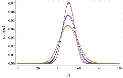
Figure 2: (Color online) Probability distributions $p_{r}(n)$ (dark yellow diamonds) and $p_{l}(n)$ (magenta squares) calculated on the basis of Eq. (90) for $\delta=0$, $\Omega_{r}=\sqrt{2}\Gamma$, and $\langle N_{r}\rangle=\langle N_{l}\rangle=\frac{\Gamma\tau}{4}=50$. Blue circles indicate the Poissonian distribution with the same mean value. Solid lines correspond to the Gaussian approximations $\frac{e^{-\frac{(n-\langle N_{r}\rangle)^{2}}{2\langle N_{r}\rangle(1+Q_{r})}}}{\sqrt{2\pi\langle N_{r}\rangle(1+Q_{r})}}$ (dark yellow), $\frac{e^{-\frac{(n-\langle N_{r}\rangle)^{2}}{2\langle N_{r}\rangle}}}{\sqrt{2\pi\langle N_{r}\rangle}}$ (blue), and $\frac{e^{-\frac{(n-\langle N_{r}\rangle)^{2}}{2\langle N_{r}\rangle(1+Q_{l})}}}{\sqrt{2\pi\langle N_{r}\rangle(1+Q_{l})}}$ (magenta), which become rather accurate at large mean values. The Mandel’s $Q$-factors, which are $Q_{r}=\frac{5}{8}$ and $Q_{l}=-\frac{3}{8}$ for the chosen parameters, quantify deviations of the variances from that of the Poissonian distribution.

Deviations of (90) from the Poissonian statistics can be quantified in terms of the Mandel’s $Q$-factor Mandel

$$Q=\lim_{\tau\to\infty}\frac{\langle N^{(2)}\rangle-\langle N\rangle^{2}}{\langle N\rangle},$$ (91)

where $\langle N^{(2)}\rangle$ is the second factorial moment. For $Q<0$ a distribution is narrower than the Poissonian, and it is called sub-Poissonian; for $Q>0$ a distribution is broader than the Poissonian, and it is called super-Poissonian. If $Q=0$, a distribution is almost indistinguishable from the Poissonian. Performing an expansion of (90) in $(z-1)$ up to the quadratic term we establish

$$Q = -2\frac{Z(1-\kappa)\Gamma^{2}}{\frac{\kappa^{2}}{8}(\Omega_{r}^{2}+2\delta^{2}+2\Gamma^{2})+\Gamma^{2}(1-\kappa)}.$$ (92)

We note that in the chiral model ($\kappa=1$) the Mandel’s $Q$-factor identically vanishes, rendering it Poissonian. Considering $\kappa=0$ and $\kappa=2$, we find the factors $Q_{l}$ and $Q_{r}$ for the reflected and transmitted photons (recall again the necessary replacement $z-1\to\frac{z_{0}-1}{2}$)

$$Q_{l} = \frac{1}{2}Q_{\kappa=0}=-\Omega_{r}^{2}\frac{3\Gamma^{2}-\delta^{2}}{(\Omega_{r}^{2}+2\delta^{2}+2\Gamma^{2})^{2}},$$ (93)

$$Q_{r} = \frac{1}{2}Q_{\kappa=2}=\frac{\Omega_{r}^{2}\Gamma^{2}}{\frac{1}{2}\Omega_{r}^{2}+\delta^{2}}\frac{2\Omega_{r}^{2}+5\delta^{2}+\Gamma^{2}}{(\Omega_{r}^{2}+2\delta^{2}+2\Gamma^{2})^{2}}.$$ (94)

We see that for $\delta<\Gamma\sqrt{3}$ the statistics of the reflected photons is sub-Poissonian, and it turns into super-Poissonian for $\delta>\Gamma\sqrt{3}$, while the statistics of the transmitted photons is always super-Poissonian. At $\delta=0$ the expression (93) coincides with the original result of Mandel Mandel for the photon number statistics in the stationary resonance fluorescence.

In Fig. 2 we show the probability distributions $p_{r}(n)$ and $p_{l}(n)$ of transmitted and reflected photons for the long counting time $\tau=\frac{200}{\Gamma}$, which are generated by (90). We also choose $\delta=0$ and $\Omega_{r}=\sqrt{2}\Gamma$, which provide $\langle N_{r}\rangle=\langle N_{l}\rangle$, to ease a comparison of these two distributions. This plot elucidates the physical meaning of the Mandel’s $Q$-factor.

We also mention that these theoretical results on photon statistics are supported by the recent measurements of the second-order correlation function chal1 showing photon antibunching in the reflected field and superbunching in the transmitted field.

V Transmission, reflection, and the Mollow triplet

The mean field and the resonance fluorescence power spectrum, also known as the Mollow triplet Mollow , are usually computed using the equation of motion method and the quantum regression theorem. In this section we demonstrate how to obtain these expressions in the framework of our scattering approach.

To compute the mean field $\langle a(z_{1})\rangle$ and the first order correlation function $g^{(1)}(z^{\prime}_{1},z_{1})=\langle a^{\dagger}(z^{\prime}_{1})a(z_{1})\rangle$ we employ the expression (58), in which we replace $e^{i\chi N_{\tau}}$ by $a(z_{1})$ and $a^{\dagger}(z^{\prime}_{1})a(z_{1})$. Thus,

$$\langle a(z_{1})\rangle = \langle 0|S_{\alpha}^{\dagger}D^{\dagger}(\kappa\alpha)a(z_{1})D(\kappa\alpha)S_{\alpha}|0\rangle$$ (95)

$$= \frac{\kappa\alpha}{\sqrt{L}}e^{ik_{0}z_{1}}+\langle 0|S_{\alpha}^{\dagger}a(z_{1})S_{\alpha}|0\rangle,$$

$$\langle a^{\dagger}(z^{\prime}_{1})a(z_{1})\rangle = \langle 0|S_{\alpha}^{\dagger}D^{\dagger}(\kappa\alpha)a^{\dagger}(z^{\prime}_{1})a(z_{1})D(\kappa\alpha)S_{\alpha}|0\rangle$$ (96)

$$= \frac{\kappa^{2}|\alpha|^{2}}{L}e^{-ik_{0}(z^{\prime}_{1}-z_{1})}$$

$$+ \frac{\kappa\alpha^{*}}{\sqrt{L}}e^{-ik_{0}z^{\prime}_{1}}\langle a(z_{1})\rangle+\langle a(z^{\prime}_{1})\rangle^{*}\frac{\kappa\alpha}{\sqrt{L}}e^{ik_{0}z_{1}}$$

$$+ \langle 0|S_{\alpha}^{\dagger}a^{\dagger}(z^{\prime}_{1})a(z_{1})S_{\alpha}|0\rangle.$$

Note that to find the reflected and transmitted ($\kappa=0,2$) fields and their $g^{(1)}$ functions, it is necessary to multiply (95) and (96) additionally by the factors $1/\sqrt{2}$ and $1/2$.

So we see that it suffices to compute

$$\langle 0|S_{\alpha}^{\dagger}a(z_{1})S_{\alpha}|0\rangle$$

$$= \langle 0|S_{\alpha}^{a\,\dagger}[L/2,-L/2]a(z_{1})S_{\alpha}^{a}[L/2,-L/2]|0\rangle$$

$$+ \frac{|\lambda|^{2}}{2\Gamma}\langle 0|S_{\alpha}^{b\,\dagger}[L/2,-L/2]a(z_{1})S_{\alpha}^{b}[L/2,-L/2]|0\rangle$$

and

$$\tilde{g}^{(1)}(z^{\prime}_{1},z_{1})\equiv\langle 0|S_{\alpha}^{\dagger}a^{\dagger}(z^{\prime}_{1})a(z_{1})S_{\alpha}|0\rangle$$

$$= \langle 0|S_{\alpha}^{a\,\dagger}[L/2,-L/2]a^{\dagger}(z^{\prime}_{1})a(z_{1})S_{\alpha}^{a}[L/2,-L/2]|0\rangle$$

$$+ \frac{|\lambda|^{2}}{2\Gamma}\langle 0|S_{\alpha}^{b\,\dagger}[L/2,-L/2]a^{\dagger}(z^{\prime}_{1})a(z_{1})S_{\alpha}^{b}[z_{1},-L/2]|0\rangle.$$

Applying the $\alpha$-shifted versions of (19) and (20) we obtain

$$\langle 0|S_{\alpha}^{\dagger}a(z_{1})S_{\alpha}|0\rangle = \lambda e^{ik_{0}z_{1}}$$

$$\times\left(\langle 0|S_{\alpha}^{a\,\dagger}[L/2,-L/2]\right.$$

$$\qquad\times S_{\alpha}^{b}[L/2,z_{1}]S_{\alpha}^{a}[z_{1},-L/2]|0\rangle$$

$$+ \frac{|\lambda|^{2}}{2\Gamma}\langle 0|S_{\alpha}^{b\,\dagger}[L/2,-L/2]$$

$$\left.\qquad\times S_{\alpha}^{b}[L/2,z_{1}]S_{\alpha}^{b}[z_{1},-L/2]|0\rangle\right)$$

and

$$\tilde{g}^{(1)}(z^{\prime}_{1},z_{1}) = |\lambda|^{2}e^{-ik_{0}(z^{\prime}_{1}-z_{1})}$$

$$\times\left(\langle 0|S_{\alpha}^{a\,\dagger}[z^{\prime}_{1},-L/2]S_{\alpha}^{b\,\dagger}[L/2,z^{\prime}_{1}]\right.$$

$$\qquad\times S_{\alpha}^{b}[L/2,z_{1}]S_{\alpha}^{a}[z_{1},-L/2]|0\rangle$$

$$+ \frac{|\lambda|^{2}}{2\Gamma}\langle 0|S_{\alpha}^{b\,\dagger}[z^{\prime}_{1},-L/2]S_{\alpha}^{b\,\dagger}[L/2,z^{\prime}_{1}]$$

$$\left.\qquad\times S_{\alpha}^{b}[L/2,z_{1}]S_{\alpha}^{b}[z_{1},-L/2]|0\rangle\right).$$

Next, using (18) we split in the first case the operators $S_{\alpha}^{a,b\,\dagger}[L/2,-L/2]$ into the subintervals $[-L/2,z_{1}]$ and $[z_{1},L/2]$. Assuming $z^{\prime}_{1}>z_{1}$ in the second case, we split the operators $S_{\alpha}^{a,b\,\dagger}[z^{\prime}_{1},-L/2]$ into the subintervals $[-L/2,z_{1}]$ and $[z_{1},z^{\prime}_{1}]$ and the operator $S_{\alpha}^{b}[L/2,z_{1}]$ into the subintervals $[z_{1},z^{\prime}_{1}]$ and $[z^{\prime}_{1},L/2]$. After that, we apply the Wick’s theorem, use the identities (77)-(79), and obtain

$$\langle 0|S_{\alpha}^{\dagger}a(z_{1})S_{\alpha}|0\rangle=\lambda e^{ik_{0}z_{1}}C(L/2-z_{1}),$$

$$\tilde{g}^{(1)}(z^{\prime}_{1},z_{1})=|\lambda|^{2}e^{-ik_{0}(z^{\prime}_{1}-z_{1})}$$

$$\times \left(R(T)M(z^{\prime}_{1}-z_{1})+[C^{*}(T)-R(T)]C(z^{\prime}_{1}-z_{1})\right),$$

where $T=L/2-z^{\prime}_{1}$ and $M(\tau)=\bar{\mathcal{G}}_{a\bar{a}}(\tau)$. The properties of the latter function are studied in the Appendix E.

In the stationary regime $L/2-z_{1}\to\infty$ the mean field equals

$$\langle a(z_{1})\rangle\approx e^{ik_{0}z_{1}}\left(\frac{\kappa\alpha}{\sqrt{L}}+\frac{\lambda\Gamma}{\Gamma+|\lambda|^{2}}\right).$$ (99)

In particular, we find the mean reflected ($\kappa=0$) and transmitted ($\kappa=2$) fields (recall also about the additional factor $1/\sqrt{2}$)

$$\langle a_{l}(z_{1})\rangle \approx -\frac{\alpha_{0}e^{ik_{0}z_{1}}}{\sqrt{L}}\frac{i\Gamma(\delta-i\Gamma)}{\frac{1}{2}\Omega_{r}^{2}+\delta^{2}+\Gamma^{2}},$$ (100)

$$\langle a_{r}(z_{1})\rangle \approx \frac{\alpha_{0}e^{ik_{0}z_{1}}}{\sqrt{L}}\left(1-\frac{i\Gamma(\delta-i\Gamma)}{\frac{1}{2}\Omega_{r}^{2}+\delta^{2}+\Gamma^{2}}\right).$$ (101)

Dividing these expressions by $\frac{\alpha_{0}e^{ik_{0}z_{1}}}{\sqrt{L}}$, we obtain the reflection and transmission amplitudes, in full agreement with coherent1 and coherent2 .

We note that for the strong drive the quantities $|\langle a_{l/r}(z_{1})\rangle|^{2}$ differ from the mean numbers of photons per unit time $N_{l/r}/\tau$, defined by (86), (87). These observables begin to coincide in the limit of the weak driving field $\alpha_{0}\to 0$ and $\Omega_{r}\to 0$, both converging to the single-photon reflection $\frac{\Gamma^{2}}{\delta^{2}+\Gamma^{2}}\frac{|\alpha_{0}|^{2}}{L}$ and transmission $\frac{\delta^{2}}{\delta^{2}+\Gamma^{2}}\frac{|\alpha_{0}|^{2}}{L}$ probabilities (times the incident photon density), what indicates the suppression of the inelastic scattering processes.

The information about the inelastic – Mollow – part of the power spectrum is contained in $\tilde{g}^{(1)}(z^{\prime}_{1},z_{1})$ expressed by (V), and, more precisely, in the functions

$$M(\tau) = \int\frac{dp}{2\pi}e^{-ip\tau}\left[\tilde{r}(p)+\frac{|\lambda|^{2}\bar{c}(p)c(p)}{1-|\lambda|^{2}r(p)}\right]$$

$$= \frac{\Gamma}{\Gamma+|\lambda|^{2}}\left(1+\frac{|\lambda|^{2}}{\Gamma}\int\frac{dp}{2\pi}e^{-ip\tau}\frac{iM_{0}(p)}{R_{0}(p)}\right),$$

$$C(\tau) = \int\frac{dp}{2\pi}e^{-ip\tau}\frac{c(p)}{1-|\lambda|^{2}r(p)}$$

$$= \frac{\Gamma}{\Gamma+|\lambda|^{2}}\left(1-\int\frac{dp}{2\pi}e^{-ip\tau}\frac{iC_{0}(p)}{R_{0}(p)}\right),$$

in the form of terms containing the third-order polynomial $R_{0}(p)$ which is defined in (76). Here $r(p)=r(p;\alpha,\alpha^{*})$, $\tilde{r}(p)=\tilde{r}(p;\alpha,\alpha^{*})$, $c(p)=c(p;\alpha,\alpha^{*})$ are the special cases of the functions (174), (175), (177), and

$$M_{0}(p)=(p+2i\Gamma)^{2}-\frac{\Omega_{r}^{2}}{2},$$ (104)

$$C_{0}(p)=M_{0}(p)-\frac{\Gamma+|\lambda|^{2}}{\Gamma}(\delta+i\Gamma)(p+2i\Gamma).$$ (105)

We note the inelastic power spectrum is the same (up to the factor $1/2$) for the chiral and reflected/transmitted photons, therefore it is sufficient to consider only the chiral case.

We analyze first the stationary regime $T\to\infty$ of (V). Here we have $R(\infty)=C(\infty)=\frac{\Gamma}{\Gamma+|\lambda|^{2}}$, and the Mollow spectrum is completely defined by $\frac{\Gamma}{\Gamma+|\lambda|^{2}}\mathrm{Re}\frac{iM_{0}(p)}{R_{0}(p)}$, in the full agreement with the known results Mollow , KM-rev . The roots of $R_{0}(p)$ define the positions and widths of all three Mollow peaks, while the functions $M_{0}(p)$ [Eq. (104)] contribute to their weights.

The expression (V) shows how the shape of the Mollow spectrum evolves in time $T$ toward its stationary value discussed above. At $T=0$ we have $R(0)=C(0)=0$, and the inelastic power spectrum is absent. For finite $T>0$ its weight starts to grow, it acquires the three-peak form, however its transient shape differs from the stationary one due to the presence of the additional contribution in $C_{0}(p)$ [Eq. (105)] which is not proportional to $M_{0}(p)$.

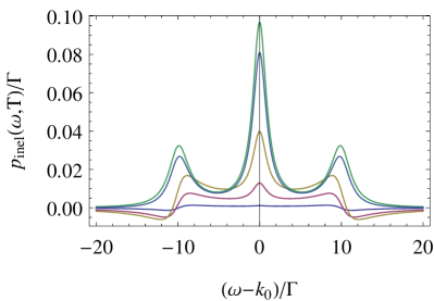
Figure 3: (Color online) Evolution of the Mollow triplet (from bottom to top) with increasing time $T=\frac{0.01}{\Gamma},\frac{0.05}{\Gamma},\frac{0.1}{\Gamma},\frac{1}{\Gamma},\frac{10}{\Gamma}$ for the parameters $\Omega_{r}=10\Gamma$ and $\delta=0$. For $T=\frac{10}{\Gamma}$ (top green curve) it is already indistinguishable from the stationary shape given by Eq. (112).

In the formal expression the power spectrum amounts to

$$P(\omega) = \frac{k_{0}}{2\pi T_{0}}\int dz^{\prime}_{1}dz_{1}\langle a^{\dagger}(z^{\prime}_{1})a(z_{1})\rangle e^{i\omega(z^{\prime}_{1}-z_{1})}$$ (106)

$$= \frac{k_{0}}{2\pi T_{0}}\mathrm{Re}\int_{0}^{T_{0}}dT\int_{0}^{\infty}d\tau e^{i\omega\tau}$$

$$\times\langle a^{\dagger}(L/2-T)a(L/2-T-\tau)\rangle,$$

where $T_{0}$ is the maximal waiting time. The inelastic part of (106) equals

$$P_{\mathrm{inel}}(\omega) = \frac{k_{0}|\lambda|^{2}}{2\pi T_{0}}\mathrm{Re}\int_{0}^{T_{0}}dT\int_{0}^{\infty}d\tau e^{i(\omega-k_{0})\tau}$$

$$\times(R(T)M_{\mathrm{inel}}(\tau)+[C^{*}(T)-R(T)]C_{\mathrm{inel}}(\tau)),$$

where

$$M_{\mathrm{inel}}(\tau) = \frac{|\lambda|^{2}}{\Gamma+|\lambda|^{2}}\int\frac{dp}{2\pi}e^{-ip\tau}\frac{iM_{0}(p)}{R_{0}(p)},$$ (108)

$$C_{\mathrm{inel}}(\tau) = -\frac{\Gamma}{\Gamma+|\lambda|^{2}}\int\frac{dp}{2\pi}e^{-ip\tau}\frac{iC_{0}(p)}{R_{0}(p)}.$$ (109)

Computing (V) we obtain

$$P_{\mathrm{inel}}(\omega) = \frac{k_{0}}{T_{0}}\int_{0}^{T_{0}}dTp_{\mathrm{inel}}(\omega,T),$$ (110)

$$p_{\mathrm{inel}}(\omega,T) = \frac{|\lambda|^{4}R(T)}{2\pi(\Gamma+|\lambda|^{2})}\mathrm{Re}\left\{\frac{iM_{0}(\omega-k_{0})}{R_{0}(\omega-k_{0})}\right\}$$

$$-\mathrm{Re}\frac{|\lambda|^{2}\Gamma[C^{*}(T)-R(T)]iC_{0}(\omega-k_{0})}{2\pi(\Gamma+|\lambda|^{2})R_{0}(\omega-k_{0})}.$$

For $T_{0}\to\infty$ we recover the stationary Mollow spectrum

$$P_{\mathrm{inel}}^{\mathrm{stat}}(\omega) = k_{0}\,p_{\mathrm{inel}}(\omega,\infty)$$ (112)

$$= \frac{k_{0}|\lambda|^{4}\Gamma}{2\pi(\Gamma+|\lambda|^{2})^{2}}\mathrm{Re}\left\{\frac{iM_{0}(\omega-k_{0})}{R_{0}(\omega-k_{0})}\right\}.$$

At large Rabi frequency $\Omega_{r}\gg\Gamma,\delta$ it acquires the most familiar form

$$P_{\mathrm{inel}}^{\mathrm{stat}}(\omega)=\frac{k_{0}\Gamma}{4\pi}$$

$$\times \left\{\frac{\Gamma}{(\omega-k_{0})^{2}+\Gamma^{2}}+\frac{1}{2}\sum_{s=\pm}\frac{\frac{3\Gamma}{2}}{(\omega-k_{0}-s\Omega_{r})^{2}+\frac{9\Gamma^{2}}{4}}\right\}.$$

For finite $T_{0}$ we show in Fig. 3 the augmentation of $p_{\mathrm{inel}}(\omega,T)$ with increasing time $T$.

VI Reduced density matrix and entanglement entropy

Explicit knowledge of the scattering state allows us to determine a reduced density matrix of some spatial interval, which we continue to call a counting interval. It suffices to trace out “past” and “future” states of the full density matrix $(S_{0}|\alpha\rangle)(\langle\alpha|S_{0}^{\dagger})$ by a procedure similar to that described in the section IV.2. Knowing the reduced density matrix, whose computation by other methods is questionable, we can study the entanglement entropy in our model.

Let us consider an arbitrary many-body operator $\hat{A}$ in the chiral model which is defined on the counting interval $[z_{1},z_{2}]$. Its average value in the scattering state reads

$$\langle\hat{A}\rangle = \langle 0|D^{\dagger}(\alpha)S_{0}^{\dagger}\hat{A}S_{0}D(\alpha)|0\rangle$$

$$= \langle 0|S_{\alpha}^{\dagger}D^{\dagger}(\alpha)\hat{A}D(\alpha)S_{\alpha}|0\rangle$$

$$= \langle 0|S_{\alpha}^{a\,\dagger}[L/2,-L/2]\hat{A}_{\alpha}S_{\alpha}^{a}[L/2,-L/2]|0\rangle$$

$$+ \frac{|\lambda|^{2}}{2\Gamma}\langle 0|S_{\alpha}^{b\,\dagger}[L/2,-L/2]\hat{A}_{\alpha}S_{\alpha}^{b}[L/2,-L/2]|0\rangle,$$

where $\hat{A}_{\alpha}=D^{\dagger}(\alpha)\hat{A}D(\alpha)$. Repeating the same steps following Eq. (150), we obtain an expression for $\langle\hat{A}_{\alpha}\rangle$ analogous to (64) – it is only necessary to set $\kappa=1$ and $z=1$, and to replace $e^{i\chi N_{\tau}}$ by $\hat{A}_{\alpha}$. This implies that $\hat{A}$ can be expressed as a trace $\mathrm{Tr}_{\tau}(\hat{A}\hat{\rho}_{\tau})$ over the states in the spatial interval $\tau=z_{2}-z_{1}$ with the reduced density matrix of this interval

$$\hat{\rho}_{\tau} = \left[1+\left(1-\frac{|\lambda|^{2}}{2\Gamma}\right)R(T)-2\mathrm{Re}\,C(T)\right]$$ (115)

$$\times \left(|\psi^{a}\rangle\langle\psi^{a}|+\frac{|\lambda|^{2}}{2\Gamma}|\psi^{b}\rangle\langle\psi^{b}|\right)$$

$$+ R(T)\left(|\psi^{c}\rangle\langle\psi^{c}|+\frac{|\lambda|^{2}}{2\Gamma}|\psi^{\bar{a}}\rangle\langle\psi^{\bar{a}}|\right)$$

$$+ \left[C(T)-R(T)\right]\left(|\psi^{a}\rangle\langle\psi^{c}|+\frac{|\lambda|^{2}}{2\Gamma}|\psi^{b}\rangle\langle\psi^{\bar{a}}|\right)$$

$$+ \left[C^{*}(T)-R(T)\right]\left(|\psi^{c}\rangle\langle\psi^{a}|+\frac{|\lambda|^{2}}{2\Gamma}|\psi^{\bar{a}}\rangle\langle\psi^{b}|\right)$$

$$= \sum_{\beta,\beta^{\prime}}\rho_{\beta\beta^{\prime}}(T)|\psi^{\beta}\rangle\langle\psi^{\beta^{\prime}}|,$$

where

$$|\psi^{\beta}\rangle=D(\alpha)S^{\beta}_{\alpha}[z_{2},z_{1}]|0\rangle$$ (116)

are linearly independent many-body states. Thus, it turns out that $\hat{\rho}_{\tau}$ describes the states in the effective four-dimensional Hilbert space spanned by $|\psi^{\beta}\rangle$. The reduced density matrix (115) is characterized by four eigenvalues $\lambda_{i}$, and the entanglement entropy of the interval $\tau$ with the rest of the pulse is then given by

$$\mathcal{S}=-\sum_{i=1}^{4}\lambda_{i}\ln\lambda_{i}.$$ (117)

The basis (116) is, however, not orthonormal, and the corresponding Gram matrix $\langle\psi^{\gamma^{\prime}}|\psi^{\gamma}\rangle$ differs from the identity. Our central observation is that its components coincide with the two-point functions (48), $\langle\psi^{\gamma^{\prime}}|\psi^{\gamma}\rangle=\bar{\mathcal{G}}_{\gamma^{\prime}\gamma}(\tau)$. Therefore, the eigenvalues $\lambda_{i}$ coincide with the eigenvalues of the $4\times 4$ matrix $\rho(T)\bar{\mathcal{G}}(\tau)$.

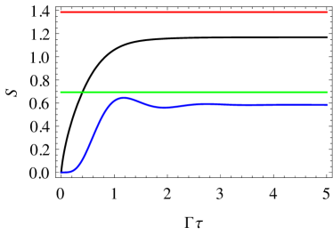
Figure 4: (Color online) Entanglement entropy $\mathcal{S}$ as a function of the subsystem size $\tau$ for $T\to\infty$ (black upper curve) and $T=0$ (blue lower curve); the detuning $\delta=0$ and the Rabi frequency $\Omega_{r}=4\Gamma$ are the same for both curves. The horizontal lines indicate the limiting values $\ln 4$ (upper line) and $\ln 2$ (lower line).

In the bulk regime $T\to\infty$ we find that one of the eigenvalues of the matrix $\rho(\infty)\bar{\mathcal{G}}(\tau)$ equals

$$\lambda_{4}(\tau)=-\frac{|\lambda|^{4}R(\tau)}{4\Gamma(\Gamma+|\lambda|^{2})}-|\lambda|^{2}\frac{M(\tau)-1}{2(\Gamma+|\lambda|^{2})}.$$ (118)

At small $\tau$ we have

$$\lambda_{1}(\tau) \approx 1-\frac{|\lambda|^{4}\Gamma\tau}{(\Gamma+|\lambda|^{2})^{2}},$$ (119)

$$\lambda_{2}(\tau) \approx \frac{|\lambda|^{4}\Gamma\tau}{(\Gamma+|\lambda|^{2})^{2}},$$ (120)

$$\lambda_{3}(\tau) \sim O(\tau^{2}),$$ (121)

$$\lambda_{4}(\tau) \sim O(\tau^{3}),$$ (122)

which leads us to the following behavior of the entanglement entropy

$$\mathcal{S}_{\infty}\approx-\frac{|\lambda|^{4}}{(\Gamma+|\lambda|^{2})^{2}}(\Gamma\tau)\ln(\Gamma\tau).$$ (123)

In the limit of large $\tau\to\infty$ we have

$$\lambda_{1,2}=\frac{1}{4}\left(1\pm\sigma\right)^{2},\quad\lambda_{3}=\lambda_{4}=\frac{1-\sigma^{2}}{4},$$ (124)

where

$$\sigma=\frac{\sqrt{\Gamma(\Gamma+2|\lambda|^{2})}}{\Gamma+|\lambda|^{2}}<1,$$ (125)

leading us to the expression

$$\mathcal{S}_{\infty}^{\infty} = \lim_{\tau\to\infty}\mathcal{S}_{\infty}$$ (126)

$$= -(1+\sigma)\ln\frac{1+\sigma}{2}-(1-\sigma)\ln\frac{1-\sigma}{2}.$$

For the weak drive $|\lambda|^{2}\ll\Gamma$ ($\sigma\to 1$), $\mathcal{S}_{\infty}^{\infty}$ vanishes. It means that in the absence of inelastic processes there are no correlations, and therefore there is no entanglement. For the strong drive $|\lambda|^{2}\gg\Gamma$ ($\sigma\to 0$) we obtain $\lambda_{i}\approx\frac{1}{4}$, and $\mathcal{S}_{\infty}^{\infty}$ approaches its maximal upper bound $\ln 4$.

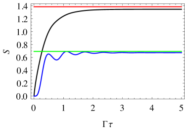
Figure 5: (Color online) The same quantities as in Fig. 4 for the different Rabi frequency $\Omega_{r}=10\Gamma$.

In the boundary regime $T=0$ the rank of $\rho(0)$ reduces by two (because of $R(0)=C(0)=0$), and we have only two nonzero eigenvalues

$$\lambda_{1,2}(\tau)=\frac{1}{2}\left(1\pm\sqrt{\left(1-\frac{|\lambda|^{2}}{\Gamma}R(\tau)\right)^{2}-2\frac{|\lambda|^{2}}{\Gamma}|C(\tau)|^{2}}\right).$$

(127)

At small $\tau$ they behave like

$$\lambda_{1}\approx 1-\frac{(\Omega_{r}\tau)^{2}}{2},\quad\lambda_{2}\approx\frac{(\Omega_{r}\tau)^{2}}{2},$$ (128)

yielding

$$\mathcal{S}_{0}\approx-(\Omega_{r}\tau)^{2}\ln(\Omega_{r}\tau).$$ (129)

At large $\tau$ the eigenvalues (127) saturate at the values

$$\lambda_{1,2}=\frac{1\pm\sigma}{2},$$ (130)

and therefore

$$\mathcal{S}_{0}^{\infty} = \lim_{\tau\to\infty}\mathcal{S}_{0}$$ (131)

$$= -\frac{1+\sigma}{2}\ln\frac{1+\sigma}{2}-\frac{1-\sigma}{2}\ln\frac{1-\sigma}{2}.$$

It is remarkable that

$$\mathcal{S}_{0}^{\infty}=\frac{1}{2}\mathcal{S}_{\infty}^{\infty},$$ (132)

which means that the subsystem lying deep in the bulk of the scattered pulse is twice stronger entangled with the rest system than the subsystem at the forefront of the pulse. The existence of the finite values (126) and (131) in the large-$\tau$ limit tells us that the area law is asymptotically fulfilled for the large subsystem size. In our 1D geometry, the “area” of the subinterval consists either of two points in the bulk case or of a single point in the boundary case, and this difference in the “area” measure is accounted by the factor $1/2$ in (132).

At small $\tau$, the expression (123) and (129) contain the logarithmic terms, which means that the entanglement entropy for the small subsystem size violates the volume ($\sim\tau$) law in our model.

In Fig. 4 and 5 the $\tau$-dependence of the entanglement entropy for the bulk (black curve) and boundary (blue curve) cases using the values $\Omega_{r}=4\Gamma$ (moderate drive) and $\Omega_{r}=10\Gamma$ (strong drive). The upper limits $\ln 4$ and $\ln 2$ are indicated by the horizontal lines. In both cases we set the detuning $\delta=0$ for simplicity.

We observe that the bulk entanglement entropy is the monotonously growing function of the subsystem size. In turn, the boundary entanglement entropy exhibits oscillatory behavior before it reaches the saturation value. For the strong driving field both entropies nearly reach the corresponding maximally allowed values $\ln 4$ and $\ln 2$ at large $\tau$.

Our numerical analysis also shows that the entanglement entropies $\mathcal{S}(\tau)$ for finite values of $T$ lie between the blue and the black curves (not shown in Figs. 4 and 5), though not always being bounded by them, but always being bounded by $\ln 4$ from above.

VII Conclusion

We have exactly computed the full counting statistics in the fundamental quantum optical setup – a finite size pulse of the coherent light propagating in the multi-mode waveguide and interacting with the two-level system. These results provide a quantitative determination of many-body correlation effects of photons mediated by their interaction with the emitter. Our analysis takes into account the spatial parameters of the incident pulse as well as the parameters of the detector – the waiting time $T$ and the counting time $\tau$, in terms of which the FCS is defined and analyzed. We show that the three types of counting statistics for the reflected, transmitted, and chiral photons have qualitatively different behavior (sub-Poissonian, super-Poissonian, and Poissonian). We have analyzed the entanglement entropy of a spatial part of the scattered pulse with the rest of it in the chiral model, and observed the fulfillment of the area law for large subsystem size and the violation of the volume law for small subsystem size, as well as the oscillatory behavior of the entanglement entropy as a function of the subsystem size $\tau$ in the case of the short waiting time $T$.

We believe that the full characterization of properties of the scattered coherent light presented here will be requested in future theoretical and experimental studies of many-body effects in fundamental models of quantum nanophotonics and extended for more complicated systems.

Appendix A Additional details of the dressing procedure (36)

In the expression (III.3)-(III.3) we introduced the dressed propagators $d_{v}$, $\tilde{d}_{v}$, and $\tilde{\tilde{d}}_{v}$, which emerge after the re-organization of the series for $S_{v}^{\beta}[y,x]$ and are themselves defined by the following series

$$d_{v}(y-x)\! \!=\! \!d_{0}(y-x)+\sum_{n=1}^{\infty}\left(\frac{\lambda v^{*}}{\sqrt{L}}\right)^{n}\!\!\!\int{\cal D}x_{n}d_{0}(y-x_{n})$$

$$\times \!\!d_{0}(x_{n}-x_{n-1})\ldots d_{0}(x_{2}-x_{1})d_{0}(x_{1}-x),$$

$$\tilde{d}_{v}(y-x) \!=\! 1+\sum_{n=1}^{\infty}\left(\frac{\lambda v^{*}}{\sqrt{L}}\right)^{n}\int{\cal D}x_{n}$$

$$\times d_{0}(x_{n}-x_{n-1})\ldots d_{0}(x_{2}-x_{1})d_{0}(x_{1}-x)$$

$$= 1+\sum_{n=1}^{\infty}\left(\frac{\lambda v^{*}}{\sqrt{L}}\right)^{n}\int{\cal D}x_{n}$$

$$\times d_{0}(y-x_{n})d_{0}(x_{n}-x_{n-1})\ldots d_{0}(x_{2}-x_{1}),$$

$$\tilde{\tilde{d}}_{v}(y-x) = 1+\frac{\lambda v^{*}}{\sqrt{L}}(y-x)+\sum_{n=2}^{\infty}\left(\frac{\lambda v^{*}}{\sqrt{L}}\right)^{n}\int{\cal D}x_{n}$$ (135)

$$\times d_{0}(x_{n}-x_{n-1})\ldots d_{0}(x_{2}-x_{1}).$$

These functions obey the following differential equations

$$d^{\prime}_{v}(x)-i(\delta+i\Gamma)[d_{v}(x)-\tilde{d}_{v}(x)]=0,$$ (136)

$$\tilde{d}^{\prime}_{v}(x)=\frac{\lambda v^{*}}{\sqrt{L}}d_{v}(x),$$ (137)

$$\tilde{\tilde{d}}^{\prime}_{v}(x)=\frac{\lambda v^{*}}{\sqrt{L}}\tilde{d}_{v}(x),$$ (138)

$$d_{v}(0)=0,$$ (139)

$$\tilde{d}_{v}(0)=\tilde{\tilde{d}}_{v}(0)=1.$$ (140)

Solving them, we find (42)-(44).

Appendix B Derivation of (64)

It is easy to check the following commutation relations

$$\,[\bar{b}_{k_{0}},\bar{b}_{k_{0}}^{\dagger}] = \frac{\tau}{L},$$ (141)

$$\,[\bar{b}_{k_{0}},\tilde{b}_{k_{0}}^{\dagger}] = 0,$$ (142)

$$\,[\tilde{b}_{k_{0}},\tilde{b}_{k_{0}}^{\dagger}] = 1-\frac{\tau}{L},$$ (143)

as well as

$$\,[N_{\tau},\bar{b}_{k_{0}}] = -\bar{b}_{k_{0}},\quad[N_{\tau},\bar{b}_{k_{0}}^{\dagger}]=\bar{b}^{\dagger}_{k_{0}},$$ (144)

$$\,[N_{\tau},\tilde{b}_{k_{0}}] = [N_{\tau},\tilde{b}_{k_{0}}^{\dagger}]=0.$$ (145)

Accounting them in application of the Baker-Campbell-Hausdorff formula, we establish the identity

$$e^{i\chi N_{\tau}}e^{\kappa\alpha b_{k_{0}}^{\dagger}}=e^{\kappa\alpha\tilde{b}_{k_{0}}^{\dagger}}e^{\kappa\alpha z\bar{b}_{k_{0}}^{\dagger}}e^{i\chi N_{\tau}},$$ (146)

where $z=e^{i\chi}$. Next, we define $\bar{B}=\sqrt{\frac{L}{\tau}}\bar{b}_{k_{0}}$ and $\tilde{B}=\sqrt{\frac{L}{L-\tau}}\tilde{b}_{k_{0}}$, such that $[\bar{B},\bar{B}^{\dagger}]=[\tilde{B},\tilde{B}^{\dagger}]=1$, and establish

$$e^{\kappa\alpha^{*}b_{k_{0}}}e^{\kappa\alpha\tilde{b}_{k_{0}}^{\dagger}}e^{\kappa\alpha z\bar{b}_{k_{0}}^{\dagger}}$$ (147)

$$= e^{\kappa\alpha^{*}\sqrt{\frac{\tau}{L}}\bar{B}}e^{\kappa\alpha z\sqrt{\frac{\tau}{L}}\bar{B}^{\dagger}}e^{\kappa\alpha^{*}\sqrt{\frac{L-\tau}{L}}\tilde{B}}e^{\kappa\alpha\sqrt{\frac{L-\tau}{L}}\tilde{B}^{\dagger}}$$

$$= e^{z\kappa^{2}|\alpha|^{2}\frac{\tau}{L}+\kappa^{2}|\alpha|^{2}\frac{L-\tau}{L}}e^{\kappa\alpha z\sqrt{\frac{\tau}{L}}\bar{B}^{\dagger}}e^{\kappa\alpha^{*}\sqrt{\frac{\tau}{L}}\bar{B}}$$

$$\times e^{\kappa\alpha\sqrt{\frac{L-\tau}{L}}\tilde{B}^{\dagger}}e^{\kappa\alpha^{*}\sqrt{\frac{L-\tau}{L}}\tilde{B}}$$

$$= e^{z\kappa^{2}|\alpha|^{2}\frac{\tau}{L}+\kappa^{2}|\alpha|^{2}\frac{L-\tau}{L}}e^{\kappa\alpha z\bar{b}^{\dagger}_{k_{0}}}e^{\kappa\alpha\tilde{b}_{k_{0}}^{\dagger}}e^{\kappa\alpha^{*}b_{k_{0}}}.$$

Finally, using the identity analogous to (146)

$$e^{\kappa\alpha^{*}b_{k_{0}}}e^{i\chi N_{\tau}}=e^{i\chi N_{\tau}}e^{\kappa\alpha^{*}\tilde{b}_{k_{0}}}e^{\kappa\alpha^{*}z\bar{b}_{k_{0}}},$$ (148)

and combining the result together with (146) and (147), we obtain the expression

$$e^{\kappa\alpha^{*}b_{k_{0}}}e^{i\chi N_{\tau}}e^{\kappa\alpha b_{k_{0}}^{\dagger}}=e^{z\kappa^{2}|\alpha|^{2}\frac{\tau}{L}+\kappa^{2}|\alpha|^{2}\frac{L-\tau}{L}}$$

$$\times e^{\kappa\alpha z\bar{b}^{\dagger}_{k_{0}}}e^{\kappa\alpha\tilde{b}_{k_{0}}^{\dagger}}e^{i\chi N_{\tau}}e^{\kappa\alpha^{*}\tilde{b}_{k_{0}}}e^{\kappa\alpha^{*}z\bar{b}_{k_{0}}},$$ (149)

whose rhs contains the exponents of annihilation (creation) operators standing to the right (left) from $e^{i\chi N_{\tau}}$, in contrast to the original reciprocal arrangement appearing in lhs of this expression. Inserting (149) into (59), we deduce

$$F_{\tau}^{(\kappa)}(\chi)e^{-(z-1)\kappa^{2}|\alpha|^{2}\frac{\tau}{L}}$$ (150)

$$= \langle 0|S_{0}^{\dagger}e^{z_{\kappa}\alpha\bar{b}^{\dagger}_{k_{0}}}e^{\alpha\tilde{b}_{k_{0}}^{\dagger}}e^{i\chi N_{\tau}}e^{z_{\kappa}\alpha^{*}\bar{b}_{k_{0}}}e^{\alpha^{*}\tilde{b}_{k_{0}}}S_{0}|0\rangle$$

$$= \langle 0|S_{0}^{a\,\dagger}[L/2,-L/2]e^{\alpha b_{k_{0}}^{f\,\dagger}}e^{z_{\kappa}\alpha\bar{b}^{\dagger}_{k_{0}}}e^{\alpha b_{k_{0}}^{p\,\dagger}}$$

$$\times e^{i\chi N_{\tau}}e^{\alpha^{*}b_{k_{0}}^{p}}e^{z_{\kappa}\alpha^{*}\bar{b}_{k_{0}}}e^{\alpha^{*}b_{k_{0}}^{f}}S_{0}^{a}[L/2,-L/2]|0\rangle$$

$$+ \frac{|\lambda|^{2}}{2\Gamma}\langle 0|S_{0}^{b\,\dagger}[L/2,-L/2]e^{\alpha b_{k_{0}}^{f\,\dagger}}e^{z_{\kappa}\alpha\bar{b}^{\dagger}_{k_{0}}}e^{\alpha b_{k_{0}}^{p\,\dagger}}$$

$$\times e^{i\chi N_{\tau}}e^{\alpha^{*}b_{k_{0}}^{p}}e^{z_{\kappa}\alpha^{*}\bar{b}_{k_{0}}}e^{\alpha^{*}b_{k_{0}}^{f}}S_{0}^{b}[L/2,-L/2]|0\rangle,$$

where $z_{\kappa}=\kappa(z-1)+1$.

The result of counting should not depend on the “future” – this is a manifestation of the causality principle. Therefore, we expect that (150) identically equals

$$F_{\tau}^{(\kappa)}(\chi)e^{-(z-1)\kappa^{2}|\alpha|^{2}\frac{\tau}{L}}$$ (151)

$$= \langle 0|S_{0}^{a\,\dagger}[L/2,z_{1}]e^{z_{\kappa}\alpha\bar{b}^{\dagger}_{k_{0}}}e^{\alpha b_{k_{0}}^{p\,\dagger}}$$

$$\times e^{i\chi N_{\tau}}e^{\alpha^{*}b_{k_{0}}^{p}}e^{z_{\kappa}\alpha^{*}\bar{b}_{k_{0}}}S_{0}^{a}[L/2,z_{1}]|0\rangle$$

$$+ \frac{|\lambda|^{2}}{2\Gamma}\langle 0|S_{0}^{b\,\dagger}[L/2,z_{1}]e^{z_{\kappa}\alpha\bar{b}^{\dagger}_{k_{0}}}e^{\alpha b_{k_{0}}^{p\,\dagger}}$$

$$\times e^{i\chi N_{\tau}}e^{\alpha^{*}b_{k_{0}}^{p}}e^{z_{\kappa}\alpha^{*}\bar{b}_{k_{0}}}S_{0}^{b}[L/2,z_{1}]|0\rangle.$$

This statement can be rigorously proven using the splitting relations (18). The identities (77)-(79) appear essential for such a proof.

In the next step we integrate out the fields in the “past”. They do influence the counting, therefore the result of this procedure can not be simply guessed. To eliminate the “past” fields in a systematic way, we employ the first and the second relations of (18), splitting the interval $[z_{1},L/2]$ into the counting $\tau=z_{2}-z_{1}$ and the “past” (or waiting) $T=L/2-z_{2}$ subintervals. Applying the Wick’s theorem separately on each subinterval, we obtain the formula (64).

Appendix C Laplace transforms (70)

The explicit expressions for the Laplace transforms (70) are obtained by the resummation of geometric series in the Laplace space which emerge from the unique possibility for the Wick’s contraction of the path-ordered field operators. The result of this procedure reads

$$\mathcal{G}_{aa}(p) = \mathcal{G}_{\bar{a}\bar{a}}(p)=\frac{\tilde{r}(p;u,v^{*})}{1-|\lambda|^{2}r(p;u,v^{*})},$$ (152)

$$\mathcal{G}_{bb}(p) = \frac{r(p;u,v^{*})}{1-|\lambda|^{2}r(p;u,v^{*})},$$ (153)

$$\mathcal{G}_{cc}(p) = \tilde{\tilde{r}}(p;u,v^{*})+\frac{|\lambda|^{2}\tilde{r}^{2}(p;u,v^{*})}{1-|\lambda|^{2}r(p;u,v^{*})},$$ (154)

$$\mathcal{G}_{\bar{a}b}(p) = \mathcal{G}_{ab}(p)=\frac{c(p;u,v^{*})}{1-|\lambda|^{2}r(p;u,v^{*})},$$ (155)

$$\mathcal{G}_{b\bar{a}}(p) = \mathcal{G}_{ba}(p)=\frac{\bar{c}(p;u,v^{*})}{1-|\lambda|^{2}r(p;u,v^{*})},$$ (156)

$$\mathcal{G}_{ca}(p) = \mathcal{G}_{c\bar{a}}(p)=b(p;u,v^{*})$$ (157)

$$\qquad+\frac{|\lambda|^{2}c(p;u,v^{*})\tilde{r}(p;u,v^{*})}{1-|\lambda|^{2}r(p;u,v^{*})},$$

$$\mathcal{G}_{ac}(p) = \mathcal{G}_{\bar{a}c}(p)=\bar{b}(p;u,v^{*})$$ (158)

$$\qquad+\frac{|\lambda|^{2}\bar{c}(p;u,v^{*})\tilde{r}(p;u,v^{*})}{1-|\lambda|^{2}r(p;u,v^{*})},$$

$$\mathcal{G}_{a\bar{a}}(p) = \tilde{r}(p;u,v^{*})+\frac{|\lambda|^{2}c(p;u,v^{*})\bar{c}(p;u,v^{*})}{1-|\lambda|^{2}r(p;u,v^{*})},$$ (159)

$$\mathcal{G}_{cb}(p) = f(p;u,v^{*})+\frac{|\lambda|^{2}c(p;u,v^{*})c(p;u,v^{*})}{1-|\lambda|^{2}r(p;u,v^{*})},$$ (160)

$$\mathcal{G}_{bc}(p) = \bar{f}(p;u,v^{*})+\frac{|\lambda|^{2}\bar{c}(p;u,v^{*})\bar{c}(p;u,v^{*})}{1-|\lambda|^{2}r(p;u,v^{*})},$$ (161)

where the functions

$$r(p;u,v^{*}) = \int_{0}^{\infty}dx\,d_{u}^{*}(x)d_{v}(x)e^{ipx},$$ (162)

$$\tilde{r}(p;u,v^{*}) = \int_{0}^{\infty}dx\,\tilde{d}_{u}^{*}(x)\tilde{d}_{v}(x)e^{ipx},$$ (163)

$$\tilde{\tilde{r}}(p;u,v^{*}) = \int_{0}^{\infty}dx\,\tilde{\tilde{d}}_{u}^{*}(x)\tilde{\tilde{d}}_{v}(x)e^{ipx},$$ (164)

$$c(p;u,v^{*}) = \int_{0}^{\infty}dx\,\tilde{d}_{u}^{*}(x)d_{v}(x)e^{ipx},$$ (165)

$$\bar{c}(p;u,v^{*}) = \int_{0}^{\infty}dx\,d_{u}^{*}(x)\tilde{d}_{v}(x)e^{ipx},$$ (166)

$$b(p;u,v^{*}) = \int_{0}^{\infty}dx\,\tilde{\tilde{d}}_{u}^{*}(x)\tilde{d}_{v}(x)e^{ipx},$$ (167)

$$\bar{b}(p;u,v^{*}) = \int_{0}^{\infty}dx\,\tilde{d}_{u}^{*}(x)\tilde{\tilde{d}}_{v}(x)e^{ipx},$$ (168)

$$f(p;u,v^{*}) = \int_{0}^{\infty}dx\,\tilde{\tilde{d}}^{*}_{u}(x)d_{v}(x)e^{ipx},$$ (169)

$$\bar{f}(p;u,v^{*}) = \int_{0}^{\infty}dx\,d^{*}_{u}(x)\tilde{\tilde{d}}_{v}(x)e^{ipx}$$ (170)

are obtained using the explicit form of the functions $d_{v}(x)$, $\tilde{d}_{v}(x)$, $\tilde{\tilde{d}}_{v}(x)$ from Eqs. (42),(43),(44).

Appendix D Computation of (IV.2)-(IV.2)

To compute the quantities in (IV.2)-(IV.2), we insert into (72) the expressions for $\mathcal{G}_{\beta^{\prime}\beta}(p)$ from the Appendix C and obtain

$$\Lambda_{aa}(\tau)+\frac{|\lambda|^{2}}{2\Gamma}\Lambda_{bb}(\tau)$$

$$= \int\frac{dp}{2\pi}e^{-ip\tau}\frac{\tilde{r}(p;z_{\kappa}\alpha,z_{\kappa}\alpha^{*})+\frac{|\lambda|^{2}}{2\Gamma}r(p;z_{\kappa}\alpha,z_{\kappa}\alpha^{*})}{1-z|\lambda|^{2}r(p;z_{\kappa}\alpha,z_{\kappa}\alpha^{*})},$$

$$\Lambda_{cc}(\tau)+\frac{|\lambda|^{2}}{2\Gamma}\Lambda_{\bar{a}\bar{a}}(\tau)$$

$$= \int\frac{dp}{2\pi}e^{-ip\tau}\left[\tilde{\tilde{r}}(p;z_{\kappa}\alpha,z_{\kappa}\alpha^{*})+\frac{|\lambda|^{2}}{2\Gamma}\tilde{r}(p;z_{\kappa}\alpha,z_{\kappa}\alpha^{*})\right.$$

$$\left.\qquad\qquad\times\frac{1+2\Gamma z\tilde{r}(p;z_{\kappa}\alpha,z_{\kappa}\alpha^{*})}{1-z|\lambda|^{2}r(p;z_{\kappa}\alpha,z_{\kappa}\alpha^{*})}\right],$$

$$\Lambda_{ca}(\tau)+\frac{|\lambda|^{2}}{2\Gamma}\Lambda_{\bar{a}b}(\tau)$$

$$= \int\frac{dp}{2\pi}e^{-ip\tau}\left[b(p;z_{\kappa}\alpha,z_{\kappa}\alpha^{*})+\frac{|\lambda|^{2}}{2\Gamma}c(p;z_{\kappa}\alpha,z_{\kappa}\alpha^{*})\right.$$

$$\left.\qquad\qquad\times\frac{1+2\Gamma z\tilde{r}(p;z_{\kappa}\alpha,z_{\kappa}\alpha^{*})}{1-z|\lambda|^{2}r(p;z_{\kappa}\alpha,z_{\kappa}\alpha^{*})}\right].$$

Establishing the functions (162), (163), (164), (165), (167) for $u=z_{\kappa}\alpha$ and $v^{*}=z_{\kappa}\alpha^{*}$ in the explicit form

$$r(p;z_{\kappa}\alpha,z_{\kappa}\alpha^{*})=-\frac{2i(\delta^{2}+\Gamma^{2})(p+i\Gamma)}{Q_{0}(p,z_{\kappa})},$$ (174)

$$\tilde{r}(p;z_{\kappa}\alpha,z_{\kappa}\alpha^{*})=i\frac{R_{0}(p)-\frac{\Omega_{r}^{2}}{2}(z_{\kappa}-2)(p+i\Gamma)}{Q_{0}(p,z_{\kappa})},$$ (175)

$$\tilde{\tilde{r}}(p;z_{\kappa}\alpha,z_{\kappa}\alpha^{*})$$ (176)

$$\qquad=\frac{i}{Q_{0}(p,z_{\kappa})}\left[R_{0}(p)-iz_{\kappa}\Gamma\Omega_{r}^{2}\frac{p^{2}+\delta^{2}+\Gamma^{2}}{2(\delta^{2}+\Gamma^{2})}\right.$$

$$\left.+\Omega^{2}_{r}(p+i\Gamma)\left(1-z_{\kappa}\frac{\delta^{2}-\Gamma^{2}}{\delta^{2}+\Gamma^{2}}-z_{\kappa}^{2}\frac{\Omega_{r}^{2}}{8(\delta^{2}+\Gamma^{2})}\right)\right],$$

$$c(p;z_{\kappa}\alpha,z_{\kappa}\alpha^{*})$$ (177)

$$\qquad=\frac{i(\delta+i\Gamma)(p+2i\Gamma)(p-\delta+i\Gamma)}{Q_{0}(p,z_{\kappa})},$$

$$b(p;z_{\kappa}\alpha,z_{\kappa}\alpha^{*})=\tilde{r}(p;z_{\kappa}\alpha,z_{\kappa}\alpha^{*})$$ (178)

$$\qquad-\frac{i\Omega_{r}^{2}z_{\kappa}(p+2i\Gamma)(p+\delta+i\Gamma)}{4(\delta-i\Gamma)Q_{0}(p,z_{\kappa})},$$

where

$$Q_{0}(p,z_{\kappa}) = pR_{0}(p)-i\Gamma\Omega_{r}^{2}(p+i\Gamma)$$ (179)

$$-(z_{\kappa}-1)\Omega_{r}^{2}(p+i\Gamma)^{2},$$

and inserting them into (D)-(D), we arrive after some transformations at (IV.2)-(IV.2).

Appendix E Correlation functions (48)

Setting $u=v=\alpha$, we introduce the following notations

$$\bar{\mathcal{G}}_{bb}(\tau) = R(\tau),$$ (180)

$$\bar{\mathcal{G}}_{ab}(\tau) = \bar{\mathcal{G}}_{ba}^{*}(\tau)=C(\tau),$$ (181)

$$\bar{\mathcal{G}}_{a\bar{a}}(\tau) = M(\tau),$$ (182)

$$\bar{\mathcal{G}}_{cb}(\tau) = \bar{\mathcal{G}}_{bc}^{*}(\tau)=N(\tau).$$ (183)

From the normalization identities (77)-(79) it follows

$$\bar{\mathcal{G}}_{aa}(\tau) = \bar{\mathcal{G}}_{\bar{a}\bar{a}}(\tau)=1-\frac{|\lambda|^{2}}{2\Gamma}R(\tau),$$ (184)

$$\bar{\mathcal{G}}_{cc}(\tau) = 1+\frac{|\lambda|^{4}}{4\Gamma^{2}}R(\tau),$$ (185)

$$\bar{\mathcal{G}}_{ca}(\tau) = \bar{\mathcal{G}}_{ac}^{*}(\tau)=1-\frac{|\lambda|^{2}}{2\Gamma}C(\tau).$$ (186)

We establish the following differential equations for the functions $R(\tau)$, $C(\tau)$, $M(\tau)$, and $N(\tau)$.

The function $R(\tau)$ obeys the differential equation

$$\dddot{R}(\tau)+4\Gamma\ddot{R}(\tau)+\left(\Omega_{r}^{2}+\delta^{2}+5\Gamma^{2}\right)\dot{R}(\tau)$$

$$+\Gamma\left(\Omega_{r}^{2}+2\delta^{2}+2\Gamma^{2}\right)R(\tau)=2\Gamma\left(\delta^{2}+\Gamma^{2}\right),$$ (187)

equipped with the initial conditions $R(0)=\dot{R}(0)=0$, $\ddot{R}(0)=2(\delta^{2}+\Gamma^{2})$.

The function $M(\tau)$ obeys the same differential equation (187) equipped the initial conditions $M(0)=1$, $\dot{M}(0)=0$, $\ddot{M}(0)=-\Omega_{r}^{2}/2$.

The function $C(\tau)$ obeys the differential equation

$$\dot{C}(\tau)-i(\delta+i\Gamma)C(\tau)$$ (188)

$$= -i(\delta+i\Gamma)\left(1-\frac{\Omega_{r}^{2}}{2(\delta^{2}+\Gamma^{2})}R(\tau)\right),$$

with the initial condition $C(0)=0$.

The function $N(\tau)$ obeys the differential equation

$$\dot{N}(\tau)-i(\delta+i\Gamma)N(\tau)$$ (189)

$$= -\frac{\delta+i\Gamma}{\delta-i\Gamma}\left(\dot{M}(\tau)+i(\delta-i\Gamma)M(\tau)\right),$$

with the initial condition $N(0)=0$.

At small $\tau$ these functions have the following behavior

$$R(\tau) \approx (\delta^{2}+\Gamma^{2})\tau^{2},$$

$$C(\tau) \approx -i(\delta+i\Gamma)\tau,$$

$$M(\tau) \approx 1-\frac{\Omega_{r}^{2}\tau^{2}}{4},$$

$$N(\tau) \approx -i(\delta+i\Gamma)\tau,$$

while in the limit $\tau\to\infty$ they all reach the same stationary value $\frac{\Gamma}{\Gamma+|\lambda|^{2}}=\frac{2\delta^{2}+2\Gamma^{2}}{2\delta^{2}+2\Gamma^{2}+\Omega_{r}^{2}}$.

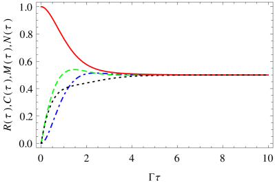
Figure 6: (Color online) The functions $R(\tau)$ (dot-dashed blue), $C(\tau)$ (dashed green), $M(\tau)$ (solid red), and $N(\tau)$ (dotted black), for $\delta=0$ and $\Omega_{r}=\sqrt{2}\Gamma$. At large $\tau$ they all saturate at the value 0.5.

In the resonant case $\delta=0$ we find the analytic solutions to these differential equations

$$R(\tau) = \frac{2\Gamma^{2}}{\Omega_{r}^{2}+2\Gamma^{2}}$$

$$- \frac{2\Gamma^{2}(\bar{\Omega}_{r}\cos\bar{\Omega}_{r}\tau+\frac{3\Gamma}{2}\sin\bar{\Omega}_{r}\tau)}{\bar{\Omega}_{r}(\Omega_{r}^{2}+2\Gamma^{2})}e^{-\frac{3\Gamma}{2}\tau},$$

$$C(\tau) = \frac{2\Gamma^{2}}{\Omega_{r}^{2}+2\Gamma^{2}}$$

$$+ \frac{\Gamma[(\Omega^{2}_{r}-\Gamma^{2})\sin\bar{\Omega}_{r}\tau-2\Gamma\bar{\Omega}_{r}\cos\bar{\Omega}_{r}\tau]}{\bar{\Omega}_{r}(\Omega_{r}^{2}+2\Gamma^{2})}e^{-\frac{3\Gamma}{2}\tau},$$

$$M(\tau) = \frac{2\Gamma^{2}}{\Omega_{r}^{2}+2\Gamma^{2}}+\frac{1}{2}e^{-\Gamma\tau}$$

$$+ \frac{\Omega_{r}^{2}-2\Gamma^{2}}{2(\Omega_{r}^{2}+2\Gamma^{2})}e^{-\frac{3\Gamma}{2}\tau}\cos\bar{\Omega}_{r}\tau$$

$$+ \frac{\Gamma}{4\bar{\Omega}_{r}}\frac{5\Omega_{r}^{2}-2\Gamma^{2}}{\Omega_{r}^{2}+2\Gamma^{2}}e^{-\frac{3\Gamma}{2}\tau}\sin\bar{\Omega}_{r}\tau,$$

$$N(\tau) = M(\tau)-e^{-\Gamma\tau},$$ (193)

where $\bar{\Omega}_{r}=\sqrt{\Omega_{r}^{2}-\frac{\Gamma^{2}}{4}}$. They are shown in Fig. 6 for $\Omega_{r}=\sqrt{2}\Gamma$.

References

- (1) A. V. Akimov, A. Mukherjee, C. L. Yu, D. E. Chang, A. S. Zibrov, P. R. Hemmer, H. Park, and M. D. Lukin, “Generation of single optical plasmons in metallic nanowires coupled to quantum dots”, Nature 450, 402 (2007).
- (2) O. Astafiev, A. M. Zagoskin, A. A. Abdumalikov Jr., Yu. A. Pashkin, T. Yamamoto, K. Inomata, Y. Nakamura, and J. S. Tsai, “Resonance Fluorescence of a Single Artificial Atom”, Science 327, 840 (2010).
- (3) B. Dayan, A. S. Parkins, T. Aoki, E. P. Ostby, K. J. Vahala, and H. J. Kimble, “A Photon Turnstile Dynamically Regulated by One Atom”, Science 319, 1062 (2008).
- (4) A. A. Abdumalikov, Jr., O. Astafiev, A. M. Zagoskin, Yu. A. Pashkin, Y. Nakamura, and J. S. Tsai, “Electromagnetically Induced Transparency on a Single Artificial Atom”, Phys. Rev. Lett. 104, 193601 (2010).
- (5) I.-C. Hoi, C. M. Wilson, G. Johansson, T. Palomaki, B. Peropadre, and P. Delsing, “Demonstration of a Single-Photon Router in the Microwave Regime”, Phys. Rev. Lett. 107, 073601 (2011).
- (6) I.-C. Hoi, T. Palomaki, J. Lindkvist, G. Johansson, P. Delsing and C. M. Wilson, “Generation of nonclassical microwave states using an artificial atom in 1D open space”, Phys. Rev. Lett. 108, 263601 (2012).
- (7) I.-C. Hoi, A. F. Kockum, T. Palomaki, T. M. Stace, B. Fan, L. Tornberg, S. R. Sathyamoorthy, G. Johansson, P. Delsing, and C. M. Wilson, “Giant Cross Kerr Effect for Propagating Microwaves Induced by an Artificial Atom”, Phys. Rev. Lett. 111, 053601 (2013).
- (8) C. Eichler, C. Lang, J. M. Fink, J. Govenius, S. Filipp, and A. Wallraff, “Observation of Entanglement between Itinerant Microwave Photons and a Superconducting Qubit”, Phys. Rev. Lett. 109, 240501 (2012).
- (9) C. Eichler, D. Bozyigit, C. Lang, L. Steffen, J. Fink, and A. Wallraff, “Experimental State Tomography of Itinerant Single Microwave Photons”, Phys. Rev. Lett. 106, 220503 (2011).
- (10) C. Santori, D. Fattal, and Y. Yamamoto, Single-photon Devices and Applications (Wiley-VCH, 2010).
- (11) M. D. Eisaman, J. Fan, A. Migdall, and S. V. Polyakov, “Single-photon sources and detectors”, Rev. Sci. Instrum. 82, 071101 (2011).
- (12) J. Claudon, J. Bleuse, N. Singh Malik, M. Bazin, P. Jaffrennou, N. Gregersen, C. Sauvan, P. Lalanne, and J.-M. Gérard, “A highly efficient single-photon source based on a quantum dot in a photonic nanowire”, Nature Photon. 4, 174 (2010).
- (13) A. Reinhard, T. Volz, M. Winger, A. Badolato, K. J. Hennessy, E. L. Hu, and A. Imamoglu, “Strongly correlated photons on a chip”, Nature Photon. 6, 93 (2012).
- (14) V. I. Rupasov, “Complete integrability of the quasi-one-dimensional quantum model of Dicke superradiance”, JETP Lett 36, 142 (1982).
- (15) V. I. Rupasov, “Contribution to the Dicke superradiance theory. Exact solution of the quasi-one-dimensional quantum model”, Sov. Phys. JETP 56, 989 (1982).
- (16) V. I. Rupasov and V. I. Yudson, “Exact Dicke superradiance theory: Bethe wavefunctions in the discrete atom model”, Sov. Phys. JETP 59, 478 (1984).
- (17) V. I. Rupasov and V. I. Yudson, “Rigorous theory of cooperative spontaneous emission of radiation from a lumped system of two-level atoms: Bethe ansatz method”, Zh. Eksp. Teor. Fiz. 87, 1617-1630 (1984), [Sov. Phys. JETP 60, 927 (1984)].
- (18) V. I. Yudson, “Dynamics of integrable quantum systems”, Zh. Eksp. Teor. Fiz. 88, 1757 (1985) [Sov. Phys. JETP 61, 1043 (1985)].
- (19) V. I. Yudson, “Dynamics of the integrable one-dimensional system: photons + two-level atoms”, Phys. Lett. A 129, 17 (1988).
- (20) V. I. Yudson, “Density matrix and entropy of scattered light in the resonance fluorescence”, Phys. Lett. A 129, 359 (1988).
- (21) A. LeClair, “QED for a Fibrillar Medium of Two-Level Atoms”, Phys. Rev. A 56, 782 (1997).
- (22) R. Konik and A. LeClair, “The Scattering Theory of Oscillator Defects in an Optical Fiber”, Phys. Rev. B 58, 1872 (1998).
- (23) A. LeClair, F. Lesage, S. Lukyanov, and H. Saleur, “The Maxwell-Bloch Theory in Quantum Optics and the Kondo Model”, Phys. Lett. A 235, 203 (1997).
- (24) A. LeClair, “Eigenstates of the Atom-Field Interaction and the Binding of Light in Photonic Crystals”, Ann. Phys. 271, 268 (1999).
- (25) M. Ringel, M. Pletyukhov, and V. Gritsev, “Topologically protected strongly correlated states of photons”, New J. Phys. 16, 113030 (2014).
- (26) S. R. Sathyamoorthy, L. Tornberg, A. F. Kockum, B. Q. Baragiola, J. Combes, C.M. Wilson, T. M. Stace, G. Johansson, “Quantum nondemolition detection of a propagating microwave photon”, Phys. Rev. Lett. 112, 093601 (2014).
- (27) K. Kojima, H. F. Hofmann, S. Takeuchi, and K. Sasaki, “Nonlinear interaction of two photons with a one-dimensional atom: Spatiotemporal quantum coherence in the emitted field”, Phys. Rev. A 68, 013803 (2003).
- (28) H. F. Hofmann, K. Kojima, S. Takeuchi, and K. Sasaki, “Entanglement and four wave mixing effects in the dissipation free nonlinear interaction of two photons at a single atom”, Phys. Rev. A 68, 043813 (2003).
- (29) K. Kojima, H. F. Hofmann, S. Takeuchi, and K. Sasaki, “A study on the shape of two-photon wavefunctions after the nonlinear interaction with a one-dimensional atom”, arXiv:quant-ph/0404119.
- (30) J.-T. Shen and S. Fan, “Coherent photon transport from spontaneous emission in one-dimensional waveguides”, Opt. Lett. 30, 2001 (2005).
- (31) J.-T. Shen and S. Fan, “Coherent single photon transport in a one-dimensional waveguide coupled with superconducting quantum bits”, Phys. Rev. Lett. 95, 213001 (2005).
- (32) J.-T. Shen and S. Fan, “Strongly correlated two photon transport in a one-dimensional waveguide coupled to a two-level system”, Phys. Rev. Lett. 98, 153003 (2007).
- (33) J.-T. Shen and S. Fan, “Strongly correlated multiparticle transport in one dimension through a quantum impurity”, Phys. Rev. A 76, 062709 (2007).
- (34) D. E. Chang, A. S. Sorensen, E. A. Demler, and M. D. Lukin, “A single-photon transistor using nanoscale surface plasmons”, Nature Phys. 3, 807 (2007).
- (35) L. Zhou, Z. R. Gong, Yu-xi Liu, C. P. Sun, and F. Nori, “Controllable Scattering of a Single Photon inside a One-Dimensional Resonator Waveguide”, Phys. Rev. Lett. 101, 100501 (2008).
- (36) V. I. Yudson and P. Reineker, “Multiphoton scattering in a one-dimensional waveguide with resonant atoms”, Phys. Rev. A 78, 052713 (2008).
- (37) D. E. Chang, V. Gritsev, G. Morigi, V. Vuletić, M. D. Lukin, and E. A. Demler, “Crystallization of strongly interacting photons in a nonlinear optical fibre”, Nature Phys. 4, 884 (2008).
- (38) P. Longo, P. Schmitteckert, and K. Busch, “Few-photon transport in low-dimensional systems: Interaction-induced radiation trapping”, Phys. Rev. Lett. 104, 023602 (2010).
- (39) D. Witthaut and A. S. Sorensen, “Photon scattering by a threelevel emitter in a one-dimensional waveguide”, New J. Phys. 12, 043052 (2010).
- (40) H. Ian, Yu-xi Liu, and F. Nori, “Tunable electromagnetically induced transparency and absorption with dressed superconducting qubits”, Phys. Rev. A 81, 063823 (2010).
- (41) H. Zheng, D. J. Gauthier, and H. U. Baranger, “Waveguide QED: Many-body bound-state effects in coherent and Fock-state scattering from a two-level system”, Phys. Rev. A 82, 063816 (2010).
- (42) D. Roy, “Two-photon scattering by a driven three-level emitter in a one-dimensional waveguide and electromagnetically induced transparency”, Phys. Rev. Lett. 106, 053601 (2011).
- (43) T. Shi, S. Fan, and C. P. Sun, “Two-photon transport in a waveguide coupled to a cavity in a two-level system”, Phys. Rev. A 84, 063803 (2011).
- (44) M. Hafezi, D. E. Chang, V. Gritsev, E. A. Demler, and M. D. Lukin, “Photonic quantum transport in a nonlinear optical fiber”, EPL 94, 54006 (2011).
- (45) H. Zheng, D. J. Gauthier, and H. U. Baranger, “Strongly correlated photons generated by coupling a three- or four-level system to a waveguide”, Phys. Rev. A 85, 043832 (2012).
- (46) M. Hafezi, D. E. Chang, V. Gritsev, E. Demler, and M. D. Lukin, “Quantum transport of strongly interacting photons in a one-dimensional nonlinear waveguide”, Phys. Rev. A 85, 013822 (2012).
- (47) Jie-Qiao Liao and C. K. Law, “Correlated two-photon transport in a one-dimensional waveguide side-coupled to a nonlinear cavity”, Phys. Rev. A 82, 053836 (2010).
- (48) Jin-Feng Huang, Jie-Qiao Liao, and C. P. Sun, “Photon blockade induced by atoms with Rydberg coupling”, Phys. Rev. A 87, 023822 (2013).
- (49) M. Pletyukhov and V. Gritsev, “Scattering of massless particles in one-dimensional chiral channel”, New J. Phys. 14, 095028 (2012).
- (50) D. Oehri, M. Pletyukhov, V. Gritsev, G. Blatter, and S. Schmidt, “Tunable, nonlinear Hong-Ou-Mandel interferometer”, Phys. Rev. A 91, 033816 (2015).
- (51) E. Sanchez-Burillo, D. Zueco, J. J. Garcia-Ripoll, and L. Martin-Moreno, “Scattering in the Ultrastrong Regime: Nonlinear Optics with One Photon”, Phys. Rev. Lett. 113, 263604 (2014).
- (52) J. F. M. Werra, P. Longo, and K. Busch, “Spectra of coherent resonant light pulses interacting with a two-level atom in a waveguide”, Phys. Rev. A 87, 063821 (2013).
- (53) Ch. Martens, P. Longo, and K. Busch, “Photon transport in one-dimensional systems coupled to three-level quantum impurities”, New J. Phys. 15, 083019 (2013).
- (54) D. Valente, Y. Li, J. P. Poizat, J. M. Gerard, L. C. Kwek, M. F. Santos, and A. Auffeves, “Optimal irreversible stimulated emission”, New J. Phys. 14, 083029 (2012).
- (55) D. Valente, S. Portolan, G. Nogues, J. P. Poizat, M. Richard, J. M. Gerard, M. F. Santos, and A. Auffeves, “Monitoring stimulated emission at the single-photon level in one-dimensional atoms”, Phys. Rev. A 85, 023811 (2012).
- (56) A. F. van Loo, A. Fedorov, K. Lalumiere, B. C. Sanders, A. Blais, and A. Wallraff, “Photon-Mediated Interactions Between Distant Artificial Atoms”, Science 342, 1494 (2013).
- (57) H. Zheng and H. U. Baranger, “Persistent Quantum Beats and Long-Distance Entanglement from Waveguide-Mediated Interactions”, Phys. Rev. Lett. 110, 113601 (2013).
- (58) M. Laakso and M. Pletyukhov, “Scattering of Two Photons from Two Distant Qubits: Exact Solution”, Phys. Rev. Lett. 113, 183601 (2014).
- (59) F. Fratini, E. Mascarenhas, L. Safari, J. P. Poizat, D. Valente, A. Auffeves, D. Gerace, and M. F. Santos, “Fabry-Perot Interferometer with Quantum Mirrors: Nonlinear Light Transport and Rectification”, Phys. Rev. Lett. 113, 243601 (2014).
- (60) A. Gonzalez-Tudela, D. Martin-Cano, E. Moreno, L. Martin-Moreno, C. Tejedor, and F. J. Garcia-Vidal, “Entanglement of Two Qubits Mediated by One-Dimensional Plasmonic Waveguides”, Phys. Rev. Lett. 106, 020501 (2011).
- (61) B. R. Mollow, “Power Spectrum of Light Scattered by Two-Level Systems”, Phys. Rev. 188, 169 (1969).
- (62) P. Knight and P.W. Milonni, “The Rabi frequency in optical spectra”, Phys. Rep. 66, 21 (1980).
- (63) R. J. Glauber, Quantum theory of optical coherence (Wiley-VCH, 2007).
- (64) R. Hanbury Brown and R. Q. Twiss, “A Test of a New Type of Stellar Interferometer on Sirius”, Nature 178, 1046 (1956).
- (65) L. Mandel and E. Wolf, Optical Coherence and Quantum Optics (Cambridge University Press, Cambridge, 1995).
- (66) P. L. Kelley and W. H. Kleiner, “Theory of Electromagnetic Field Measurement and Photoelectron Counting”, Phys. Rev. A 136, 316 (1964).
- (67) L. Mandel, “Sub-Poissonian photon statistics in resonance fluorescence”, Optics Lett., 4, 205 (1979).
- (68) R. J. Cook, “Photon number statistics in resonance fluorescence”, Phys. Rev. A 23, 1243 (1981).
- (69) D. Lenstra, “Photon-number statistics in resonance fluorescence”, Phys. Rev. A 26, 3369 (1982).
- (70) D. F. Smirnov and A. S. Troshin, “Distribution of photocounts in nonlinear resonance fluorescence”, Zh. Eksp. Theor. Phys. 81, 1597 (1981).
- (71) L. S. Levitov and G. B. Lesovik, “Charge distribution in quantum shot noise”, JETP Lett. 58, 230 (1993).
- (72) L. S. Levitov, H. Lee, and G. B. Lesovik, “Electron counting statistics and coherent states of electric current”, J. Math. Phys. 37, 4845 (1996).
- (73) Y. V. Nazarov and Ya. M. Blanter, in Quantum Transport: Introduction to Nanoscience (Cambridge UP, 2009).
- (74) W. Belzig, “Full Counting Statistics in Quantum Contacts”, arXiv:cond-mat/0312180 (2003).
- (75) D. A. Bagrets and Yu. V. Nazarov, “Full counting statistics of charge transfer in Coulomb blockade systems”, Phys. Rev. B 67, 085316 (2003).
- (76) D. A. Bagrets, Y. Utsumi, D. S. Golubev and G. Schön, “Full counting statistics of interacting electrons”, Fortschr. Phys. 54, 917 (2006).
- (77) A. O. Gogolin and A. Komnik, “Full Counting Statistics for the Kondo Dot in the Unitary Limit”, Phys. Rev. Lett. 97, 016602 (2006).
- (78) K. Schönhammer, “Full counting statistics for noninteracting fermions: Exact results and the Levitov-Lesovik formula”, Phys. Rev. B 75, 205329 (2007).
- (79) A. Komnik and H. Saleur, “Quantum Fluctuation Theorem in an Interacting Setup: Point Contacts in Fractional Quantum Hall Edge State Devices”, Phys. Rev. Lett. 107, 100601 (2011).
- (80) E. Boulat, H. Saleur, and P. Schmitteckert, “Twofold Advance in the Theoretical Understanding of Far-From-Equilibrium Properties of Interacting Nanostructures”, Phys. Rev. Lett. 101 140601 (2008).
- (81) A. Branschädel, E. Boulat, H. Saleur, and P. Schmitteckert, “Shot Noise in the Self-Dual Interacting Resonant Level Model”, Phys. Rev. Lett. 105, 146805 (2010).
- (82) S. T. Carr, D. A. Bagrets, and P. Schmitteckert, “Full Counting Statistics in the Self-Dual Interacting Resonant Level Model”, Phys. Rev. Lett. 107, 206801 (2011).
- (83) E. V. Sukhorukov and O. M. Bulashenko, “Quantum-to-Classical Crossover in Full Counting Statistics”, Phys. Rev. Lett. 94, 116803 (2005).
- (84) F. Taddei and R. Fazio, “Counting statistics for entangled electrons”, Phys. Rev. B 65, 075317 (2002).
- (85) I. Klich and L. Levitov, “Quantum Noise as an Entanglement Meter”, Phys. Rev. Lett. 102, 100502 (2009).
- (86) H. F. Song, C. Flindt, S. Rachel, I. Klich, and K. Le Hur, “Entanglement entropy from charge statistics: Exact relations for noninteracting many-body systems”, Phys. Rev. B 83, 161408(R) (2011).
- (87) D. A. Ivanov and A. G. Abanov, “Phase transitions in full counting statistics for periodic pumping”, Europhys. Lett. 92, 37008 (2010).
- (88) C. Flindt and J. P. Garrahan, “Trajectory Phase Transitions, Lee-Yang Zeros, and High-Order Cumulants in Full Counting Statistics”, Phys. Rev. Lett. 110, 050601 (2013).
- (89) V. Gritsev, E. Altman, E. Demler, and A. Polkovnikov, “Full quantum distribution of contrast in interference experiments between interacting one-dimensional Bose liquids”, Nature Phys. 2, 705 (2006).
- (90) A. Imambekov, V. Gritsev, and E. Demler, “Fundamental noise in matter interferometers”, cond-mat/0703766.
- (91) S. Hoffereberth, I. Lesanovsky, T. Schumm, A. Imambekov, V. Gritsev, E. Demler, and J. Schmiedmayer, “Probing quantum and thermal noise in an interacting many-body system”, Nature Phys. 4, 489 (2008).
- (92) A. Lamacraft and P. Fendley, “Order Parameter Statistics in the Critical Quantum Ising Chain”, Phys. Rev. Lett. 100, 165706 (2008).
- (93) T. Kitagawa, S. Pielawa, A. Imambekov, J. Schmiedmayer, V. Gritsev, and E. Demler, “Ramsey Interference in One-Dimensional Systems: The Full Distribution Function of Fringe Contrast as a Probe of Many-Body Dynamics”, Phys. Rev. Lett. 104, 255302 (2010).
- (94) M. Gring, M. Kuhnert, T. Langen, T. Kitagawa, B. Rauer, M. Schreitl, I. Mazets, D. Adu Smith, E. Demler, and J. Schmiedmayer, “Relaxation and Prethermalization in an Isolated Quantum System”, Science 337, 1318 (2012).
- (95) D. A. Ivanov and A. G. Abanov, “Characterizing correlations with full counting statistics: classical Ising and quantum XY spin chains”, Phys. Rev. E 87, 022114 (2013).
- (96) M. D. Hoogerland, M. N. J. H. Wijnands, H. A. J. Senhorst, H. C. W. Beijerinck, and K. A. H. van Leeuwen, “Photon statistics in resonance fluorescence: Results from an atomic-beam deflection experiment”, Phys. Rev. Lett. 65, 1559 (1990).
- (97) G. Bel and F. L. H. Brown, “Theory for Wavelength-Resolved Photon Emission Statistics in Single-Molecule Fluorescence Spectroscopy”, Phys. Rev. Lett. 102, 018303 (2009).
- (98) M. Vogl, G. Schaller, E. Schöll, and T. Brandes, “Equation-of-motion method for full counting statistics: Steady-state superradiance”, Phys. Rev. A 86, 033820 (2012).
- (99) J. Lindkvist and G. Johansson, “Scattering of coherent pulses on a two-level system, single-photon generation”, New J. Phys. 16, 055018 (2014).
- (100) J. Eisert, M. Cramer, and M. B. Plenio, “Colloquium: Area laws for the entanglement entropy”, Rev. Mod. Phys. 82, 277 (2010).
- (101) C. H. Bennett, G. Brassard, C. Crépeau, R. Jozsa, A. Peres, and W.K. Wootters, “Teleporting an unknown quantum state via dual classical and Einstein-Podolsky-Rosen channels”, Phys. Rev. Lett. 70, 1895 (1993).
- (102) C. H. Bennett, H. J. Bernstein, S. Popescu, and B. Schumacher, “Concentrating partial entanglement by local operations”, Phys. Rev. A 53, 2046 (1996).