The Panchromatic Hubble Andromeda Treasury XI: The Spatially-Resolved Recent Star Formation History of M31^^affiliation: Based on observations made with the NASA/ESA Hubble Space Telescope, obtained at the Space Telescope Science Institute, which is operated by the Association of Universities for Research in Astronomy, Inc., under NASA contract NAS 5-26555. These observations are associated with program #12055.

Alexia R. Lewis¹¹affiliation: Department of Astronomy, University of Washington, Box 351580, Seattle, WA 98195, USA;
arlewis@astro.washington.edu , Andrew E. Dolphin²²affiliation: Raytheon, 1151 E. Hermans Road, Tucson, AZ 85756, USA , Julianne J. Dalcanton¹¹affiliation: Department of Astronomy, University of Washington, Box 351580, Seattle, WA 98195, USA;
arlewis@astro.washington.edu , Daniel R. Weisz¹¹affiliation: Department of Astronomy, University of Washington, Box 351580, Seattle, WA 98195, USA;
arlewis@astro.washington.edu ¹²¹²affiliation: Hubble Fellow , Benjamin F. Williams¹¹affiliation: Department of Astronomy, University of Washington, Box 351580, Seattle, WA 98195, USA;
arlewis@astro.washington.edu , Eric F. Bell³³affiliation: Department of Astronomy, University of Michigan, 1085 S. University Ave., Ann Arbor, MI 48109, USA , Anil C. Seth⁴⁴affiliation: Department of Physics and Astronomy, University of Utah, Salt Lake City, UT 84112, USA , Jacob E. Simones⁵⁵affiliation: Minnesota Institute for Astrophysics, University of Minnesota, 116 Church Street SE, Minneapolis, MN 55455, USA , Evan D. Skillman⁵⁵affiliation: Minnesota Institute for Astrophysics, University of Minnesota, 116 Church Street SE, Minneapolis, MN 55455, USA , Yumi Choi¹¹affiliation: Department of Astronomy, University of Washington, Box 351580, Seattle, WA 98195, USA;
arlewis@astro.washington.edu , Morgan Fouesneau⁶⁶affiliation: Max-Planck-Institut für Astronomie, Königstul 17, D-69117 Heidelberg, Germany , Puragra Guhathakurta⁷⁷affiliation: UCO/Lick Observatory, University of California at Santa Cruz, 1156 High Street, Santa Cruz, CA 95064, USA , Lent C. Johnson¹¹affiliation: Department of Astronomy, University of Washington, Box 351580, Seattle, WA 98195, USA;
arlewis@astro.washington.edu , Jason S. Kalirai⁸⁸affiliation: Space Telescope Science Institute, 3700 San Martin Drive, Baltimore, MD 21218, USA , Adam K. Leroy⁹⁹affiliation: National Radio Astronomy Observatory, 520 Edgemont Road, Charlottesville, VA 22903, USA , Antonela Monachesi¹⁰¹⁰affiliation: Max-Planck-Institut für Astrophysik, Karl-Schwarzschild-Str. 1, D-85748 Garching, Germany , Hans-Walter Rix⁶⁶affiliation: Max-Planck-Institut für Astronomie, Königstul 17, D-69117 Heidelberg, Germany , Andreas Schruba¹¹¹¹affiliation: Max-Planck-Institut für extraterrestrische Physik, Giessenbachstrasse 1, 85748 Garching, Germany

Abstract

We measure the recent star formation history (SFH) across M31 using optical images taken with the Hubble Space Telescope as part of the Panchromatic Hubble Andromeda Treasury (PHAT). We fit the color-magnitude diagrams in $\sim$ 9000 regions that are $\sim$ 100 pc $\times$ 100 pc in projected size, covering a 0.5 square degree area ( $\sim$ 380 kpc ${}^{2}$ , deprojected) in the NE quadrant of M31. We show that the SFHs vary significantly on these small spatial scales but that there are also coherent galaxy-wide fluctuations in the SFH back to $\sim$ 500 Myr, most notably in M31’s 10-kpc star-forming ring. We find that the 10-kpc ring is at least 400 Myr old, showing ongoing star formation over the past $\sim$ 500 Myr. This indicates the presence of molecular gas in the ring over at least 2 dynamical times at this radius. We also find that the ring’s position is constant throughout this time, and is stationary at the level of 1 km s ${}^{-1}$ , although there is evidence for broadening of the ring due to diffusion of stars into the disk. Based on existing models of M31’s ring features, the lack of evolution in the ring’s position makes a collisional ring origin highly unlikely. Besides the well-known 10-kpc ring, we observe two other ring-like features. There is an outer ring structure at 15 kpc with concentrated star formation starting $\sim$ 80 Myr ago. The inner ring structure at 5 kpc has a much lower star formation rate (SFR) and therefore lower contrast against the underlying stellar disk. It was most clearly defined $\sim$ 200 Myr ago, but is much more diffuse today. We find that the global SFR has been fairly constant over the last $\sim$ 500 Myr, though it does show a small increase at 50 Myr that is 1.3 times the average SFR over the past 100 Myr. During the last $\sim$ 500 Myr, $\sim$ 60% of all SF occurs in the 10-kpc ring. Finally, we find that in the past 100 Myr, the average SFR over the PHAT survey area is $0.28\pm 0.03$ $\rm M_{\odot}$ ${\rm yr}^{-1}$ with an average deprojected intensity of $7.3\times 10^{-4}$ $\rm M_{\odot}$ ${\rm yr}^{-1}\>{\rm kpc}^{-2}$ , which yields a total SFR of $\sim$ 0.7 $\rm M_{\odot}$ ${\rm yr}^{-1}$ when extrapolated to the entire area of M31’s disk. This SFR is consistent with measurements from broadband estimates.

Subject headings:

galaxies: evolution – galaxies: individual (M31) – galaxies: star formation – galaxies: stellar content – galaxies: structure

^†^†slugcomment: Accepted April 8, 2015

1. Introduction

A galaxy’s star formation history (SFH) encodes much of the physics controlling its evolution. It tells us about the evolution of the star formation rate (SFR) throughout the galaxy, the evolution of the mass and metallicity distributions, and the movement of stars within the galaxy. In addition to the global evolution, focusing on the recent SFH ( $<$ 1 Gyr) reveals the relationships between stars and the gas and dust from which they form and can be used to constrain models of star formation (SF) propagation and/or dissolution. For this type of study to be possible, however, we first need a spatially-resolved view of the past SFH with sufficient resolution to probe the relevant physical scales.

Broad SFH constraints can be derived by looking at the properties of the galaxy population across cosmic time. However, examining the integrated properties of distant galaxies provides limited information on how individual galaxies form and evolve. While such integrated light studies benefit from large sample sizes, the final results are limited to conclusions about the SFHs of general galaxy types (e.g., based on bins of mass, luminosity, or color), and cannot say anything definitive about the physics that controls the evolution of individual galaxies.

To appropriately examine the evolution of individual galaxies, it is necessary to study well-resolved nearby galaxies for which there exists large amounts of ancillary data. With such data, one can, for example, analyze the relationship between star SF and gas in the spatially-resolved Kennicutt-Schmidt law (e.g., Kennicutt2007a; Bigiel2008a), understand the evolution of a galaxy’s gas reservoir (e.g., Leroy2008a; Schruba2010a; Bigiel2011a; Leroy2013b), and calibrate SFR indicators (e.g., Calzetti2007a; Li2013a), among many others. However, these studies have historically been restricted to using only the current SFR where ‘current’ is the average over some timescale characteristic of a given SFR indicator. These studies, therefore, cannot probe the evolution of these relationships with time or on small physical scales where the SFR indicators break down (e.g., Leroy2012a).

For a more detailed analysis of the recent SFH, resolved stellar populations are the gold standard. Using individual stars, we can examine the evolution of a galaxy archaeologically by analyzing the color-magnitude diagram (CMD) as a function of position within the galaxy. Embedded within the CMD is the history of SF and metallicity evolution of the galaxy. Although recovering this information is not completely assumption-free (we must make choices about the initial mass function (IMF), stellar models, constancy of SFR within time bins, etc), it is the only way to make a time-resolved measurement of the SFR. It also has the ability to recover the SFR on much finer physical scales.

CMD fitting has most often been used to probe low mass galaxies (e.g., Gallart1999a; Harris2004a; Cole2007a; Harris2009a; Monelli2010a; Weisz2011a; Monachesi2012a; Weisz2014a) because they are the most numerous type of galaxy in the Local Volume, which is one of the few places where galaxies can be sufficiently well resolved. The technique has been used to examine a few individual larger galaxies (e.g., Wyder1998a; Hernandez2000a; Bertelli2001a; Williams2002a; Williams2003a; Brown2006a; Brown2007a; Brown2008a; Williams2009a; Williams2010a; Gogarten2010a; Bernard2012a; Bernard2015a), but these studies have been limited to either small fields spread across the disk and/or halo or have low spatial resolution such that it is difficult to pick out detailed features present in the galaxy. This technique has never been used to contiguously and uniformly recover the recent SFH of an L ${}_{\star}$ galaxy with high resolution.

In this paper, we present the first finely spatially-resolved recent SFH of a significant part of the L ${}_{\star}$ galaxy, Andromeda (M31). M31 has been the target of many photometric (e.g., Brown2006a; Barmby2006a; Gordon2006a; Dalcanton2012a; Bernard2012a; Ford2013a; Sick2014a) and spectroscopic (e.g., Ibata2004a; Guhathakurta2006a; Kalirai2006a; Koch2008a; Gilbert2009a; Dorman2012a; Gilbert2014a) studies due to its proximity and similarity to the Milky Way. M31 is the ideal place to examine processes in L ${}_{\star}$ galaxies; it is close enough to be well resolved into stars with the Hubble Space Telescope (HST) but does not not face the same obstacles as studies in the Milky Way, which are plagued by uncertainties due to line-of-sight reddening and challenging distance measurements.

We generate maps of the recent ( $<$ 0.5 Gyr) SFH in M31 using resolved stars from recent observations of M31 taken as part of the Panchromatic Hubble Andromeda Treasury (PHAT; Dalcanton2012a). While other studies have examined the SFH in M31 using resolved stars (Williams2003a; Brown2006a; Brown2007a; Brown2008a; Davidge2012a; Bernard2012a), none have been as finely resolved as the work we present here.

With the resulting spatially- and temporally-resolved recent SFHs, we can see where stars form within the galaxy and how that SF evolves across the galaxy, whether it’s a single star-forming event or propagation across the disk. The maps also provide clues about the evolution of spatial structure on a variety of different scales; while we know a great deal about small-scale SF within molecular clouds and large-scale SF within the galactic environment, the maps we derive bridge these two scales. Recent SFHs also enable the analysis of fluctuations in the recent SFR. This is especially significant for SF relations, such as the Kennicutt-Schmidt relation (Schmidt1959a; Kennicutt1989a), which often assumes a constant SFR over the timescale of the tracer used. While this paper deals only with the SFHs themselves, it is the first in a series of papers on the SF, dust, and ISM contents of M31 on small spatial scales (Lewis et al., in prep).

This paper is organized as follows: We describe the data used in Section 2. In Section 3, we explain the method by which we recover the SFHs in each region. We present the resulting SFH maps in Section 4 and discuss features of the maps in Section 5. We summarize the results in Section LABEL:sec:conclusion.

2. PHAT Data

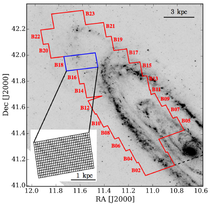
We derive the spatially resolved SFHs using photometry from the PHAT survey. PHAT surveyed the northeast quadrant of M31 in six filters, from the near-UV to the near-IR, measuring the properties of $\sim$ 117 million stars. Full details of the survey can be found in Dalcanton2012a and the photometry is described in Williams2014a. Figure 1 shows a 24 µm image (Gordon2006a) of M31 with the PHAT footprint overlaid. In this paper, we examine the SFH inside the solid red region; we have excluded the region closest to the bulge (black dashed line) where crowding errors are large and the depth of the CMD is shallow, making reliable CMD fitting difficult.

Refer to caption — Figure 1.— The PHAT NIR footprint overlaid on a 24 µm image (Gordon2006a) of M31. The thick red line denotes the area for which we compute SFHs in this paper. We have left out the regions closest to the bulge along the major axis (dashed black line) because crowding errors are large and CMD depth is shallow, which makes fitting a reliable SFH difficult. The inset shows an example of our binning scheme, shown here for Brick 18, which is outlined in blue. We have included scale bars for the large image as well as for the inset. The bricks are labeled with their numbers just exterior to the brick outline. We use these brick numbers throughout the text. The image is oriented such that north is up and east is to the left.

2.1. Photometry and Creation of Single-Brick Catalogs

We use optical photometry (F475W and F814W filters) from the .gst catalogs, which were compiled following procedures developed by Dolphin2000a as described in Dalcanton2012a. The stars in this catalog have S/N $>$ 4 in both filters and pass stringent goodness-of-fit cuts. These cuts leave stars with the highest quality photometry but with higher incompleteness in more crowded regions. The incompleteness is worse in the inner galaxy (inside $\sim$ 3 kpc), which we exclude from our analysis, and also affects the centers of stellar clusters. This latter limitation is not a problem for this paper because clusters contain only a few percent of the recent SF (Johnson et al., in prep.). Moreover, we are interested in the SFHs of the field stars, and picking out stars in the centers of dense stellar clusters is not necessary.

The survey was split into 23 regions called ‘bricks’; each brick is $\sim$ 1.5 kpc $\times$ 3 kpc in projected size. Odd-numbered bricks extend from the galactic center to the outer disk along the major axis. Even-numbered bricks sit adjacent to them at larger radii along the minor axis. Each brick is subdivided into 18 ‘fields’, each with a (projected) size of $\sim$ 500 pc $\times$ 500 pc. In the optical, adjacent fields overlap to cover the ACS chip gap. The SFHs presented in this paper are derived on a brick-by-brick basis. To create a single brick catalog from the 18 ‘field’ catalogs, we use the smaller IR brick footprint divided into 18 non-overlapping regions which roughly describe the IR field footprints. In each of these fields, we select all of the stars in the corresponding optical catalog that fall within the IR field boundaries. We fill in the chip gap using two adjacent fields, selecting only the stars that fall within the desired portion of the chip gap. Three fields in Brick 11 were not observed; this area is completely covered by overlap from Brick 09 so that there is continuous coverage over the survey area.

The result of this process is the creation of a single brick catalog of all stars detected in the optical filters that fall within the IR footprint, filling in the chip gap and eliminating duplication of stars in the overlap regions. We then grid each brick into 450 approximately equal sized, non-overlapping regions that are $\sim$ 100 pc $\times$ 100 pc in projected size for a total of $\sim$ 9000 regions across the survey area. In Figure 1, B18 is outlined in blue. The inset shows the binning scheme used within each brick.

2.2. Artificial Star Tests

Even with the resolution of HST, crowding in regions of high stellar density can strongly affect the photometry. Many faint stars cannot be resolved in the dense field of brighter stars. In addition, faint stars, that would otherwise not be detected, are biased brighter by blending with neighboring stars. This also affects brighter stars, but to a lesser degree.

To characterize photometric completeness and to account for the observational errors that result from crowding, we perform extensive artificial star tests (ASTs). Briefly, we insert fake stars into each image and run the photometry as normal. We then test for recovery of these fake stars and measure the difference between the input and recovered magnitude if a star was detected. We adopt the magnitude at which 50% of the stars are recovered as our limiting magnitude when solving for the SFHs. The completeness limits used for each brick are given in Table 1.We refer the reader to Dalcanton2012a for further details.

We inserted $\sim$ 100,000 artificial stars individually into each ACS field-of-view. We combined the resulting ASTs into brick-wide catalogs in the same way as the photometry. When running the SFHs for a given 100 pc region, we select the fake stars from a 5 $\times$ 5 grid of adjacent regions, such that the ASTs come from a 500 $\times$ 500 pc ${}^{2}$ region centered on the region of interest. Each of these larger regions contains the results of $\sim$ 50,000 ASTs.

Table 150% Completeness Limits and Isochrone Shifts

Brick	m ${}_{F475W}$	m ${}_{F814W}$	$\sigma_{\log\mathrm{T}_{\mathrm{eff}}}$	$\sigma_{\mathrm{M}_{\mathrm{bol}}}$
Number	(mag)	(mag)
02	27.2	26.1	0.019	0.22
04	27.1	25.9	0.019	0.21
05	26.4	25.0	0.019	0.18
06	27.2	26.0	0.019	0.22
07	26.8	25.4	0.019	0.18
08	27.2	26.0	0.019	0.22
09	27.1	25.8	0.019	0.21
10	27.2	26.1	0.019	0.23
11	27.1	25.9	0.019	0.21
12	27.3	26.2	0.019	0.24
13	27.2	26.1	0.019	0.23
14	27.3	26.2	0.019	0.24
15	27.4	26.2	0.019	0.25
16	27.4	26.4	0.019	0.26
17	27.5	26.4	0.020	0.26
18	27.8	26.7	0.020	0.29
19	27.6	26.7	0.020	0.28
20	27.8	26.9	0.020	0.30
21	27.8	26.9	0.020	0.30
22	27.8	26.9	0.020	0.30
23	27.8	26.9	0.020	0.30

Note. — Column 1 contains the brick number. Columns 2 and 3 list the 50% completeness limits in F475W and F814W, respectively. Columns 4 and 5 contain the shifts in $\log$ T ${}_{\mathrm{eff}}$ and M ${}_{bol}$ used when computing the systematic uncertainties.

3. Derivation of the Star Formation Histories

We derive SFHs using only the optical data from the F475W and F814W filters. These filters provide the deepest CMDs and the greatest leverage for the recent SFHs of interest in this paper. A more detailed discussion of our filter choice can be found in Appendix LABEL:app:filterchoice.

3.1. Fitting the Star Formation History

We derive the SFHs using the CMD fitting code MATCH described in Dolphin2002a. The user specifies desired ranges in age, metallicity, distance, and extinction. The code also requires a choice of IMF and a binary fraction. It then populates CMDs at each combination of age and metallicity, convolved with photometric errors and completeness as modeled by ASTs. The individual synthetic CMDs are linearly combined to form many possible SFHs. Each synthetic composite CMD is compared with the observed CMD via a Poisson maximum likelihood technique. The synthetic CMD that provides the best fit to the observed CMD is taken as the model SFH that best describes the data. For full implementation details, see Dolphin2002a.

The fit quality is given by the MATCH fit statistic: fit = $-2\ln L$ , where $L$ is the Poisson maximum likelihood. We estimate the $n\sigma$ confidence intervals as $n^{2}\geq fit-fit_{\mathrm{min}}$ ; the 1 $\sigma$ confidence interval includes all SFHs in a given region with $fit-fit_{\mathrm{min}}\leq 1$ , the 2 $\sigma$ confidence interval includes all SFHs with $fit-fit_{\mathrm{min}}\leq 4$ , etc.

We use a fixed distance modulus of 24.47 (McConnachie2005a), a binary fraction of 0.35 with the mass of the secondary drawn from a uniform distribution, and a Kroupa2001a IMF. We solve the SFH in 34 time bins covering a range in log time (in years) from 6.6 to 10.15 with a resolution of 0.1 dex except for the range of log(time) = 9.9 – 10.15 which we combine into one bin. This time binning scheme was chosen to provide as much time resolution as possible while minimizing computing time. We found that using a finer time binning scheme with a resolution of 0.05 dex increased the computing time by at least a factor of two and only resulted in differences in the SFHs of $\sim$ 1%, which is much smaller than systematic and random uncertainties. We use the Padova (Marigo2008a) isochrones with updated AGB tracks (Girardi2010a). The [M/H] range is [-2.3, 0.1] with a resolution of 0.1 dex. Because we are limited by the depth of the data, which does not reach the ancient main sequence turnoff, we also require that [M/H] only increases with time. We limit the oldest time bin to have [M/H] between -2.3 and -0.9 and the youngest time bin to have [M/H] between -0.4 and 0.1.

M31 contains significant amounts of dust (e.g., Walterbos1987a; Draine2014a; Dalcanton2015a), which, broadly speaking, can be described by three components: a mid-plane component due to extinction internal to M31 that dominates the older, well-mixed stellar populations, a foreground component due to Milky Way extinction, and a differential component that affects the star-forming regions. In addition to the SFH, MATCH allows two free parameters to describe the dust distribution: a foreground extinction ( $A_{V}$ ) and a differential extinction ( $dA_{V}$ ) which describes the spread in extinction values for the stars in each region. The differential extinction is a step function starting at $A_{V}$ with a width given by the value of $dA_{V}$ . While foreground extinction is expected to be relatively constant across the galaxy, differential extinction can vary significantly from region to region as they probe very different star-forming and stellar density environments. To determine the best fit to the data, we search extinction space to find the combination of $A_{V}$ and $dA_{V}$ that best fits the data. However, the distribution of dust is different for young stars and old stars (e.g., Zaritsky1999a). The step function differential extinction model provides a good fit to the main sequence (MS) component, but it cannot reproduce the post-MS stellar populations.

We mitigate the effects of dust on our SFHs by simplifying the fitting process such that we exclude the redder portions of the CMD from the fit. Specifically, we have adopted the cuts in Simones2014a, excluding all stars with F475W-F814W $>$ 1.25 and F475W $>$ 21 (shaded regions of the CMDs in Figures 2 and 3). This prevents contamination from the older populations. We therefore avoid extinction-related complications by excluding the RGB and the red clump, which is often poorly fit with a single step function, and which is not relevant when calculating the recent SFH.

We note that age-metallicity degeneracy is an important concern in any kind of SFH work. When modeling composite CMDs, it primarily affects the RGB (e.g., Gallart2005a), which we do not fit in this analysis. Instead, the vast majority of stars in the CMD are main sequence stars, for which the age-metallicity degeneracy is negligible compared to typical photometric uncertainties. In addition, the metallicity gradient of M31 has been extensively studied and found to be very shallow (e.g., Blair1982a; Zaritsky1994a; Galarza1999a; Trundle2002a; Kwitter2012a; Sanders2012a; Balick2013a; Lee2013a; Pilyugin2014a, Gregersen et al. in prep), and the age range we are fitting is small. As a result, we are not concerned that the age-metallicity degeneracy affects the results in this paper.

We compute the SFH in 450 regions per brick for 21 of the 23 bricks in the PHAT survey. To determine the best-fit SFH, we solve multiple SFHs with different combinations of $A_{V}$ and $dA_{V}$ , where the best-fit SFH is chosen to be the one whose combination of $A_{V}$ and $dA_{V}$ minimizes the fit value as given by the maximum likelihood technique. Consequently, for each of our regions, we must compute many possible SFHs. We minimize the total number of SFHs that must be run using an optimization scheme to limit the size of ( $A_{V}$ , $dA_{V}$ ) space that must be searched, as discussed in Appendix LABEL:app:avdav. Based on this optimization, we set a constraint that $A_{V}$ + $dA_{V}$ $\leq$ 2.5. In each region, we run a grid of SFHs in ( $A_{V}$ , $dA_{V}$ ) space with a step size of 0.3 over the range of $A_{V}$ = [0.0, 1.0], also requiring that $A_{V}$ + $dA_{V}$ $\leq$ 2.5. We take the resulting SFH with the best fit, determine the two-sigma range around that best ( $A_{V}$ , $dA_{V}$ ) pair, and then sample the grid in that region down to a finer spacing of 0.1 in $A_{V}$ and $dA_{V}$ . Not only does this ensure that we are finding the global minimum, but it also allows us to account for the uncertainty in extinction in the SFHs by including all fits in the result. In addition, the extinction parameters provide us with an additional method to verify our results, as we discuss in Section 3.2.

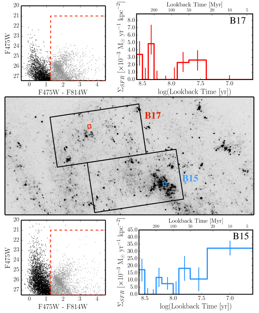
As an example, in Figure 2 we plot the CMDs and SFHs for two of the regions found near the 10-kpc ring. We show the location of these regions over-plotted on a GALEX FUV image (Gil-de-Paz2007a). The top region, in Brick 17, is located just off of a spur of the 10-kpc ring. The region itself shows very little FUV emission, and the resulting SFH is sparse with only moderate SFRs at all times. The lower region falls directly on an OB association (OB 54; vandenBergh1964a) in Brick 15. As expected, there is elevated, on-going SF in that region over at least the past 100 Myr. The CMDs for each of these regions show a well-defined MS. The consequences of dust are very evident in the region but are most easily seen in the part of the of the CMD that we do not fit, where the red clump is elongated along the reddening vector.

We note that the Padova isochrones do not include tracks younger than 4 Myr. In the resulting SFHs, we renormalize the SFR in the youngest time bin to reach the present day (0 Myr), conserving the total mass formed in that time bin.

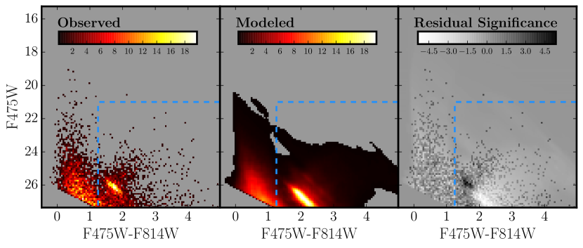
In Figure 3, we show the observed CMD, the best-fit modeled CMD, and the significance of the residuals (the observed CMD minus the modeled CMD with a weighting determined by the variance) for a region in Brick 15. We fit all stars that are outside the blue dashed region, which are primarily MS stars, with a smattering of short-lived blue helium-burning stars. The residuals show no distinct features, which means the model is a good fit.

3.2. Extinction

In this section we discuss how we incorporate IR-based dust maps as a prior in determining our dust parameters. After determining the best-fit SFH in each region as described in Section 3.1, we conducted additional verification by examining the map of total dust, $A_{V}$ + $dA_{V}$ .

We found that there were a handful of regions in which the best-fit required large amounts of dust, at or very close to the limit of 2.5 mag in spite of there being no evidence for SF within the last 100 Myr, based on a lack of luminous MS stars and low SFR averaged over the most recent 100 Myr. In these regions, we would expect very little dust because there are no dust-enshrouded young stars. Bad fits result in these cases because there are few stars in the MCD fitting region that can be used to constrain the dust.

To examine this discrepancy, we compared our dust parameters with the total dust mass in each region, as measured by Draine2014a. We correct the low-SFR, high-dust regions by constructing a prior on $A_{V}$ + $dA_{V}$ based on the Draine2014a dust mass maps and multiplying the prior by the likelihood calculated by MATCH. The details of the prior are described in Appendix LABEL:app:prior. After applying the prior, we compute new fits for all of the SFHs measured in each region. We use these new fits to go back through $A_{V}$ , $dA_{V}$ parameter space to be sure that we properly sampled 2- $\sigma$ space around the new best-fits for each region. As a result, we were able to constrain the MATCH dust parameters in the regions of very-low SFR that are not properly anchored in the CMD analysis. Ultimately, because application of the prior primarily affects the very-low SFR regions, this processing did not significantly affect the SFH results of this paper.

3.3. Uncertainties

There are three significant sources of uncertainties that affect the measured SFHs: random, systematic, and dust. In this section, we discuss each source of uncertainty in turn.

First, we consider random uncertainties. The random uncertainties are dominated by the number of stars on the CMD and are consequently larger for more sparsely populated CMDs. Random uncertainties were calculated using a hybrid Monte Carlo process (Duane1987a), implemented as described in Dolphin2013a. The result of this Markov Chain Monte Carlo routine is a sample of 10,000 SFHs with density proportional to the probability density, i.e., the density of samples is highest near the maximum likelihood point. Error bars are calculated by identifying the boundaries of the highest-density region containing 68% of the samples, corresponding to the percentage of a normal distribution falling between the $\pm 1\sigma$ bounds. This procedure provides meaningful uncertainties for time bins in which the best-fitting result indicates little or no star formation.

Next, we consider the systematic uncertainties. Systematic uncertainties reflect deficiencies in the stellar models (i.e., uncertainties due to convection, mass loss, rotation, etc.; Conroy2013a) such that different groups model these parts of stellar evolution differently, which leads to discrepant results for the same data, depending on the stellar models used (Gallart2005a; Aparicio2009a; Weisz2011a; Dolphin2012a). These uncertainties primarily affect older populations that have evolved off the MS. The stellar models of the various groups generally agree quite well for MS stars that dominate our adopted fitting region.

Because we have used the same models across the whole survey, all regions experience similar systematic effects. We have estimated the size of the systematics for a number of regions, covering the range of stellar environments within M31. We computed the systematic uncertainties by running 50 Monte Carlo realizations on the best-fit SFHs as described in Dolphin2002a. For each run, we shifted the model CMD in $\log(T_{\mathrm{eff}})$ and $M_{\mathrm{bol}}$ by an amount taken from a random draw from a Gaussian with sigma listed in Table 1. These shifts are designed to mimic differences in isochrone libraries. We then measured the resulting SFH. The range that contained 68% of the distributions from all 50 realizations is designated as the systematic uncertainties. The relative size of the systematics varies greatly from region to region but is generally less than half the size of the random uncertainties in individual regions and increases at larger lookback time. There is also more variation in the relative size of the uncertainties in the ring features than in the outermost regions where both the stellar density and the SFR are low.

Finally, the variable internal dust content introduces uncertainties. We select the best-fit SFH by choosing the ( $A_{V}$ , $dA_{V}$ ) pair that maximizes the likelihood. However, there are regions where the difference between the fit values of the two most likely SFHs is very small (i.e., both SFHs are almost equally likely). We also sample to a minimum spacing of only 0.1 in $A_{V}$ and $dA_{V}$ , and thus may have determined a slightly different best-fitting SFH than if we had sampled $A_{V}$ , $dA_{V}$ space more finely. To account for these variations, we calculate our uncertainties due to the dust distribution by combining all SFHs measured in a given region and determining the range that contains 68% of the samples. In this combination, the SFHs are weighted by their fit values such that the best-fit gets full weight and the $n\sigma$ fits are weighted by $e^{-0.5\,n^{2}}$ (e.g., SFHs with fit values that are $2\sigma$ from the best-fit value are weighted by $e^{-0.5\times 2^{2}}$ , or $e^{-2}$ ).

A possible additional source of uncertainty is due to the choice of binary fraction, which is a free parameter in this analysis. We tested the effect of different binary fractions in two of our regions and found that the final fit is not very sensitive to binary fraction. This is because the inclusion of binaries in the model results in a color separation on the CMD that is washed out by dust. The fits and resulting SFHs are consistent with the uncertainties when choosing a binary fraction anywhere between about 0.2 and 0.7. This insensitivity of the SFH to binary fraction is consistent with more extensive tests presented in Monelli2010a. Uncertainties due to binary fraction will be much smaller than those due to dust.

We note that we do not include the model systematics in our reported uncertainties. While there may be absolute uncertainties in the global SFR due to model uncertainties, the relative region-to-region uncertainties are dominated by the random and dust components.

3.4. Choice of Region Size

To generate the spatially-resolved SFH of M31, we divide each of the brick-wide catalogs into regions that are approximately 100 pc (projected; 25″) on a side, assuming a distance of 783 kpc to M31. There were a few different considerations for this size.

Regions of this size are of scientific interest because they bridge the gap between existing knowledge of Galactic pc scale SF (e.g., Bate2009a; Schruba2010a) and SF in more distant galaxies on kpc scales (e.g., Leroy2008a). The resolution is also fine enough to resolve features such as large HII regions and giant molecular clouds.

While a finer grid would also be scientifically interesting, there are a couple of difficulties to consider. The main problem is that smaller regions would have insufficiently populated CMDs, increasing the random uncertainties of the SFHs to unacceptable levels. With our adopted $\sim$ 100 pc bin size, the number of stars within the CMD fitting region ranges from 110 to 3900. In 93% of the regions, we fit more than 500 stars, and in 80% we fit more than 1000 stars. Additionally, the SFHs are computationally expensive to run. For each region, MATCH must be run multiple times to determine the ( $A_{V}$ , $dA_{V}$ ) pair that provides the best fit to the data. Moving to 50 pc size regions would have resulted in four times as many regions, significantly increasing the time needed to derive the SFHs. Even at our 100 pc grid size, deriving the SFHs and uncertainties for the entire sample required more than 500,000 CPU hours using XSEDE resources (Towns2014a).

Our overall technique is similar to that of Simones2014a, who measured the SFHs of UV-bright regions within Brick 15 of the PHAT survey. Their goal was to convert the SFHs into FUV fluxes and compare with the observed fluxes in each star-forming region. About half of their regions had fewer than 500 stars on the part of the CMD they were fitting but they still found reasonable agreement between the modeled and observed fluxes. This agreement indicates that the CMD fitting routine is robust, even with a modest number of stars in the part of the CMD occupied by young stars.

3.5. Reliability of the SFHs as a Function of Lookback Time

We have excluded the red side of the CMD in our SFH recovery process, so consequently, our fits are not sensitive to old stellar populations. The exact age at which sensitivity is lost is set by the oldest stars observable on the MS, which varies with stellar density and dust extinction.

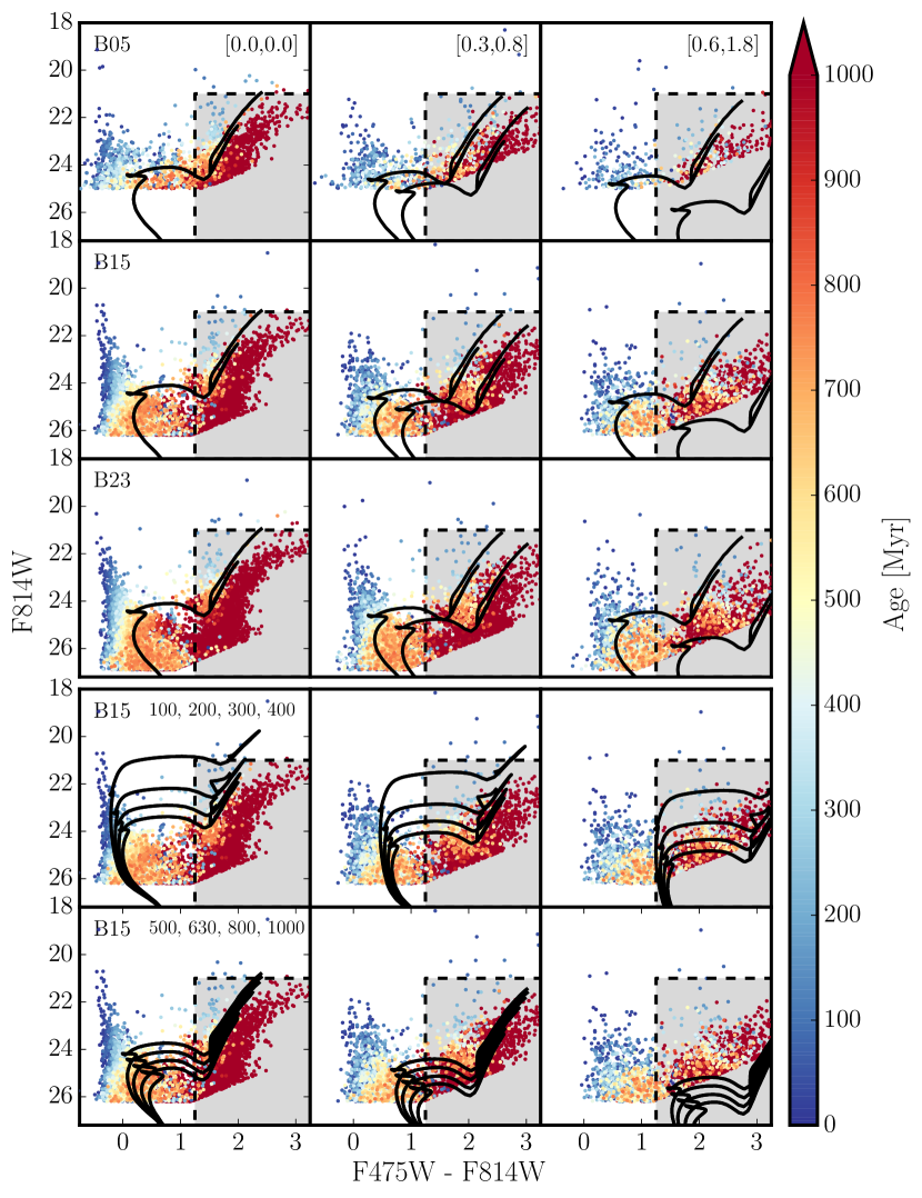
We perform two different tests to examine the sensitivity of our results as a function of time. First, we create artificial CMDs using MATCH. The CMDs are generated with a constant SFH and solar metallicity, while modeling observational uncertainties by using the results of the ASTs in each region. The results are shown in Figure 4, where we plot simulated CMDs. The youngest stars are shades of blue, and all stars older than 1 Gyr are red. Each of the top three rows shows a CMD at a different depth, where the top row is the shallowest CMD closest to the bulge (B05), and the third row is the deepest in B23. The brick numbers are indicated in the left panel. The columns display varying amounts of extinction, which is applied to the CMD in the same way we apply it to the model CMDs when recovering our SFHs. Extinction is labeled in the top panel by [ $A_{V}$ , $dA_{V}$ ]. The left column is un-reddened, the middle column shows the effect of the median extinction found in each of our regions ([ $A_{V}$ , $dA_{V}$ ] = [0.3, 0.8]), and the right column shows the upper limit of extinction allowed in our SFHs. We also check the sensitivity by over-plotting isochrones of a single age (630 Myr) and solar metallicity. The isochrone in the first column has not been reddened. In the second and third columns of the first three rows, we plot two isochrones, one extincted by $A_{V}$ and one extincted by $A_{V}$ + $dA_{V}$ . Individual stars can be extincted to anywhere between the two isochrones.

The variation in depth is large across the survey. The inner regions are very crowded and as a result the photometric depth is quite shallow. In Brick 05, where there is high crowding and moderate levels of extinction, we cannot detect many stars that are older than $\sim$ 500 Myr. As we move further away from the center of the galaxy, crowding and extinction generally decrease and we can probe stars that are 700 – 1000 Myr old (row 3 of Figure 4). The exception, of course, is the 10-kpc ring, where extinction can be high; the CMDs in the second row of Figure 4 mimic the conditions found in these regions. At low or mid-range extinction, we still see many stars on the MS that are at least 600 – 700 Myr old. As we increase the extinction, many of these stars are reddened into the portion of the CMD that we do not fit, as can also be seen from the isochrones. Unreddened 630 Myr old stars are easily recovered; however, stars that have the highest level of extinction applied to them are entirely reddened into the neglected portion of the CMD.

In the last two rows, the colored CMD is identical to that in the second row (B15 depth). Here, though, we plot solar metallicity isochrones of different ages: the fourth row has isochorones of 100, 200, 300, and 400 Myr while the bottom row shows isochrones of 500, 630, 800, and 1000 Myr. From these tests, we can see that there will be a number of regions that are reliable back to 1 Gyr, while others that are more extincted may only have a handful of stars that are more than $\sim$ 500 Myr old.

Ultimately, due to the wide variety of stellar environments found across the survey, not all bricks can reliably cover the same age range. The inner regions are much more crowded and have shallower completeness limits than the outer regions; as a result, the age limit for regions closest to the bulge is only 400 Myr. Regions that fall within the ring and spiral arm features are much more extincted than other regions; although the completeness limit is deeper, stars may be reddened into the region of the CMD that we do not fit. These regions have an age limit of no more than 500 Myr. In the outer regions where extinction and crowding are less, the completeness limit is much deeper and the SFHs are reliable back to 700 – 1000 Myr. We therefore choose a conservative age limit of 400 Myr for consistency across the survey. For all scientific analysis, we examine only the most recent 400 Myr. In some of the plots that follow, we include results back to 630 Myr for illustrative purposes, with the caveat that they are only relevant for the outermost regions of the survey.

4. Results

We now present the results of the SFH fitting process.

4.1. Star Formation Rate Maps

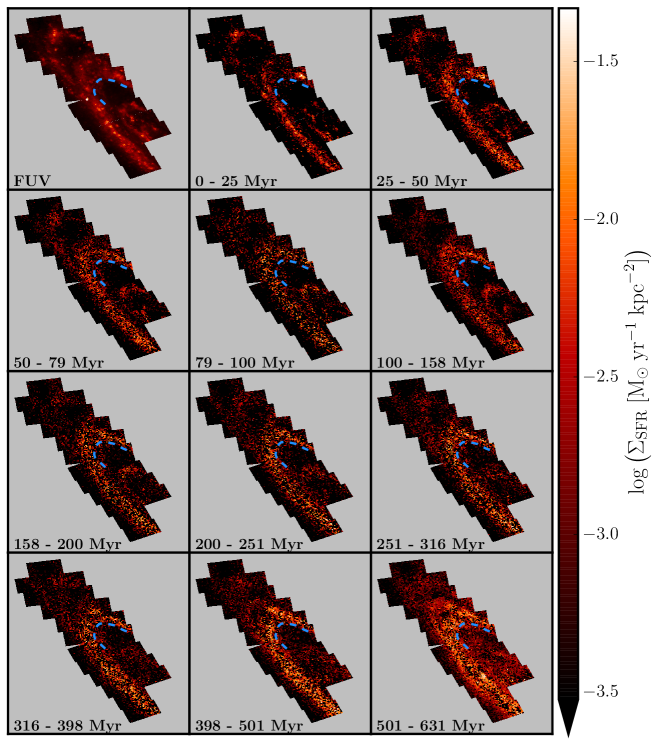
We combine the single best-fit SFHs in each region into maps of $\Sigma_{\rm SFR}$ as a function of time. As an ensemble, they reveal the recent SFH of M31 in the PHAT footprint over the last 630 Myr. This SFH is shown in Figure 5. Each panel displays the SFR surface density within the time range specified in the lower left corner. We note that these time bins are not the native resolution of $\Delta(\log t)=0.1$ ; instead, we have binned the results within the most recent 100 Myr into $\sim$ 25 Myr bins. This helps to expose the continuous structure, especially in the most recent 25 Myr when SF is very low across the galaxy. The regions are colored according to $\Sigma_{\rm SFR}$ in that region during the given time range. To more clearly illuminate the structure, we have placed a lower limit on the SFRs visible within this map such that all regions with $\Sigma_{\rm SFR}$ lower than $10^{-4}$ $\rm M_{\odot}$ ${\rm yr}^{-1}\>{\rm kpc}^{-2}$ are colored black. We have also over-plotted a blue dashed line on each image to aid the eye in recognizing structural evolution between time bins. There is little large-scale change over the last $\sim$ 500 Myr. The upper left panel shows the GALEX FUV image smoothed to the same physical scale as our SFHs, which shows excellent morphological agreement with the most recent time bins. This agreement strengthens confidence in our SFH maps given that measurements made in $\sim$ 9000 completely independent regions reproduce coherent large-scale structure seen in a well-established SFR tracer. The relationship between the SFR and the FUV flux will be examined in an upcoming paper (Simones et al. in prep.).

The SFHs reveal large-scale, long-lasting, coherent structures in the M31 disk. There are three star-forming ring-like features; a modest inner ring at $\sim$ 5 kpc, the well-known 10-kpc ring, and an outer, low-intensity ring at $\sim$ 15 kpc that partially merges with the 10-kpc ring due to a combination of projection effects and a possible warp that is visible in HI (e.g., Brinks1984a; Chemin2009a; Corbelli2010a). These rings have been observed previously in Spitzer/Infrared Array Camera (IRAC) images (Barmby2006a) and Spitzer/Multiband Imaging Photometer (MIPS) images (Gordon2006a), as well as in atomic (Brinks1984a) and molecular gas images (Nieten2006a). There is also an observed over-density of red giant branch (RGB) stars in the 10-kpc ring (Dalcanton2012a). Recovery of these coherent, well-known features is further confirmation that our method is robust.

One of the most remarkable features of this SFH is that the 10-kpc ring is visible and actively forming stars throughout the past $\sim$ 500 Myr. Although SF occurs at a low level in the outer regions at all times, SF in the ring feature at 15 kpc is most concentrated starting at 80 Myr ago. This is likely due to SF in OB 102, which has had an elevated SFR compared to its surroundings over the last $\sim$ 100 Myr (Williams2003b). The inner ring feature at $\sim$ 5 kpc is also visible, and though there appears to be SF in that ring distinct from the surrounding populations, that feature gains definition 200 Myr ago but has largely dispersed in the last 25 Myr.

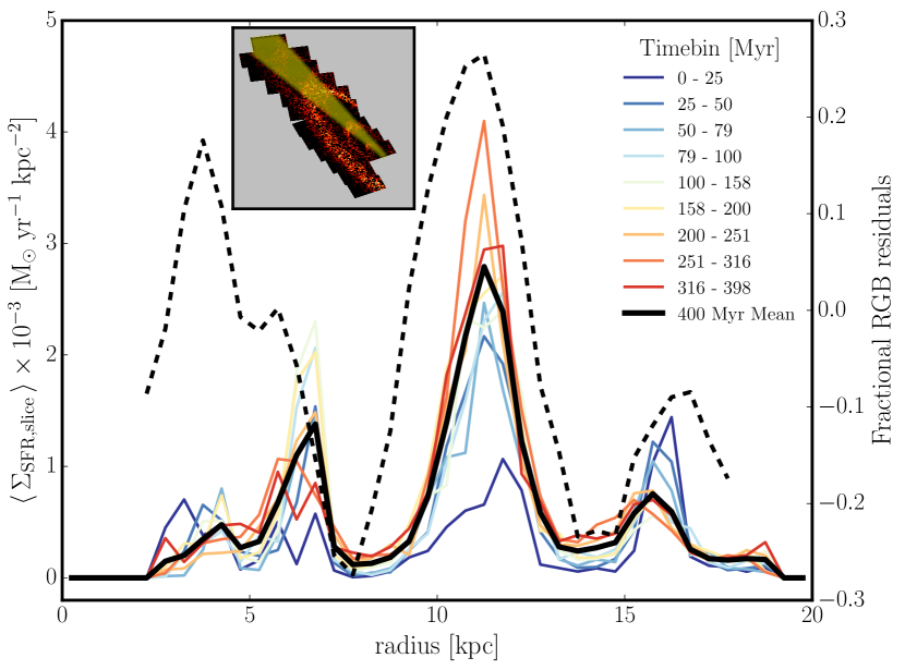
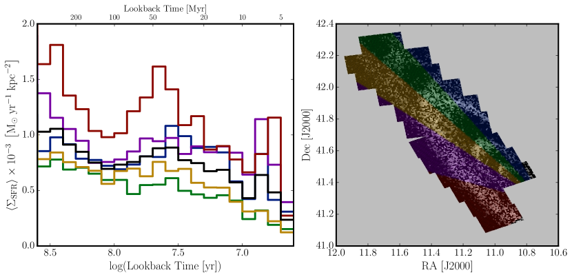
We further investigate these trends in Figure 6 where we plot the average SFR surface density as a function of radius in each time bin for a subset of the regions along the major axis. We determine the distance to the center of each region and then divide the regions into bins of 0.5 kpc. The three rings at $\sim$ 5 kpc, $\sim$ 10 kpc, and $\sim$ 15 kpc are clearly visible as peaks in $\Sigma_{\rm SFR}$ , providing further indication of ongoing (if low) SF in the ring features over 500 Myr. This trend is further supported by evidence of RGB star residuals in the ring features , as shown by the thick dashed line. There is an over density of RGB stars in the 10-kpc ring and in the inner ring where our oldest time bin shows the highest SF. The plot reveals that not only is the 10-kpc ring long-lived, it has also remained mostly stationary in galactocentric radius over 500 Myr, a result that has implications for the origin of the ring, which we discuss further in Section LABEL:subsec:ring.

4.2. Mass Maps

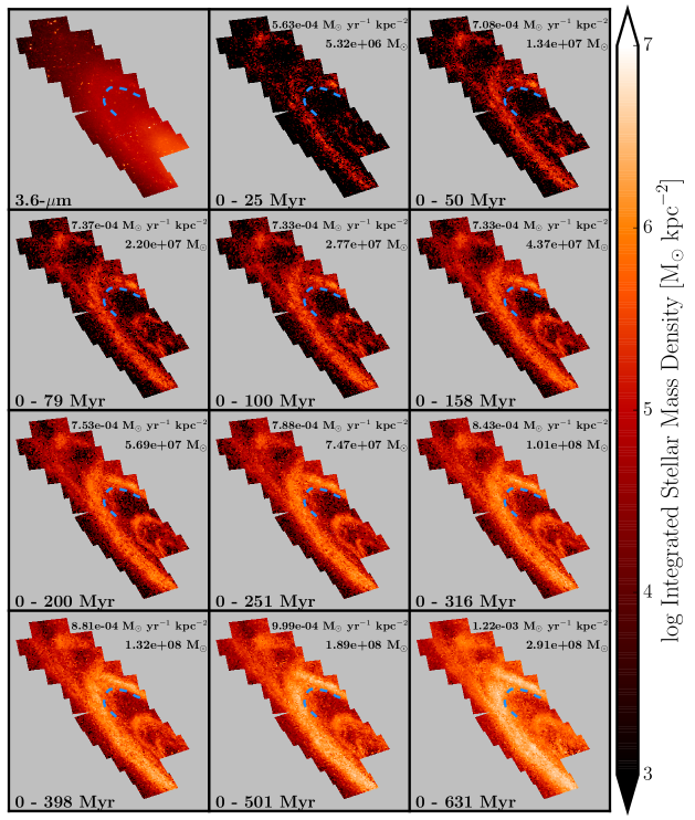
In Figure 7, we show the evolution of recent mass growth in the galaxy from 630 Myr to the present. The upper left panel shows the 3.6 µm image, which is a rough estimation of the total mass of a galaxy, smoothed to the same spatial resolution as our SFHs. The next 11 panels show the total mass formed over a given time range (the same as those in Figure 5). The upper middle panel shows the mass that formed in the last 25 Myr while the bottom right panel shows all of the mass formed in the last 630 Myr. The time range is written in the lower left of each plot. In the upper right, we have indicated the total mass formed and the average SFR over that time range.

Most of the SF in M31 occurred much earlier than the timescale probed by these SFHs; consequently, the amount of mass accumulated over the last $\sim$ 500 Myr has been minimal. As can be seen in the upper left image in Figure 7, the older stars are distributed fairly uniformly. This means that the structure that we see in our integrated mass maps only appears within the last $\sim$ 2 Gyr (more recent than the ages of stars that dominate the emission at 3.6 µm). Over the time range of our SFHs, SF has been confined primarily to the rings.

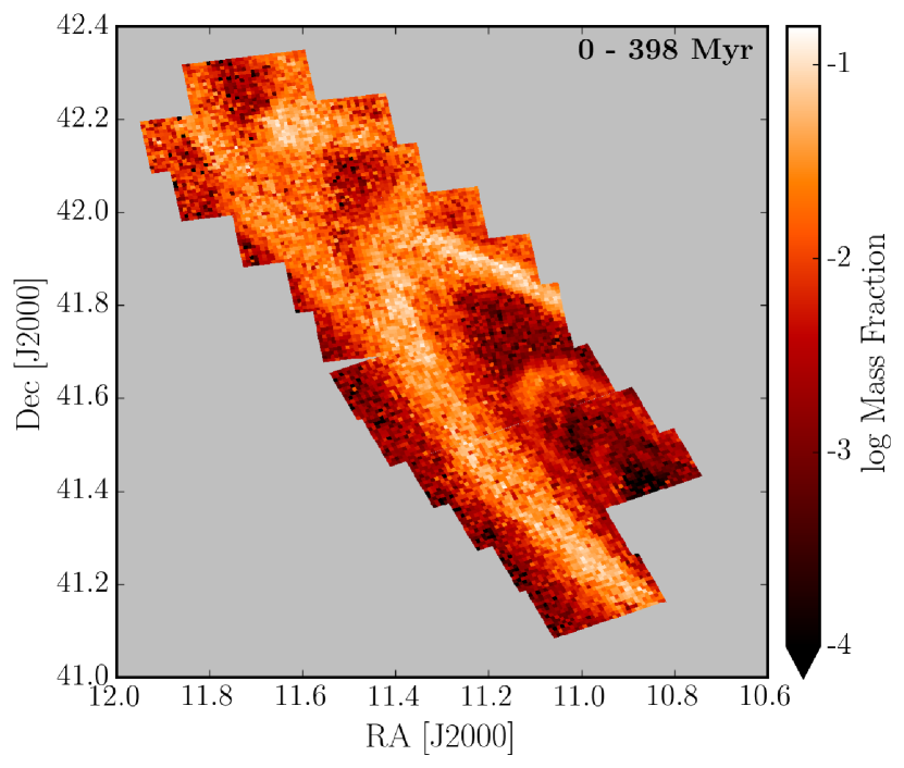
We further examine the impact of SF in the last $\sim$ 500 Myr by looking at the fraction of mass formed during this time. In Figure 8, we plot the fraction of mass formed in the last 400 Myr to the total mass in each region. We derive the total stellar mass by multiplying the 3.6 µm image (Barmby2006a) by a constant mass-to-light ratio of 0.6 (Meidt2014a). Only $\sim$ 0.8% of the total stellar mass of this section of the galaxy formed in the last 400 Myr, which is $\sim$ 3% of a Hubble time. On a region-by-region basis, the mass fraction reaches a maximum of $\sim$ 7% and is highest in the ring features, specifically in the two outer features, where most of the gas is located (see Figure 9). Consequently, though the SFR in the ring in the last $\sim$ 500 Myr is much higher than that in the rest of the galaxy, it must still be very small relative to past SFRs.

5. Discussion

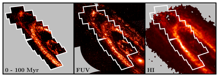
We have presented maps of SF and mass evolution in M31 that show rich structure with ongoing SF and evolution. Much of this structure has been observed in maps of M31 in other tracers. As an example, in Figure 9, we plot our SFR map averaged over the last 100 Myr, next to maps of FUV flux (Gil-de-Paz2007a) and HI (Brinks1984a). All three maps show M31’s ring structures. In addition, we note the good agreement between the 100 Myr SFR map and the map of FUV flux, which is sensitive to SF within the last 100 Myr. These regions of high SFR and flux are also broadly consistent with areas of largest gas content. We now discuss some of the features observed in these maps.

5.1. The Recent PHAT SFH

The SFHs of the individual regions are extremely diverse. Some of the regions, such as those in the 10-kpc ring have SF that is ongoing and seemingly long-lived; others, such as those that fall in the outer parts of the galaxy, have generally quiescent SFHs in the past 500 Myr. At the native time resolution of 0.1 dex, the uncertainties on the individual SFHs in each region are significant. By combining all the SFHs, we can reduce the amplitude of the uncertainties in those time bins and obtain a more significant and constrained result for the total SFH.

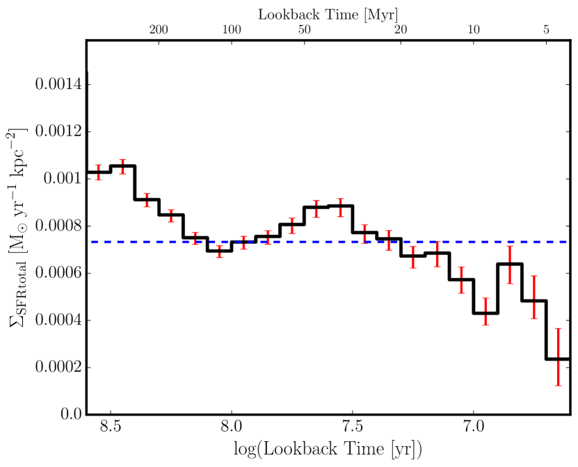
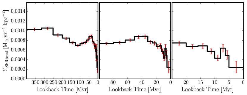
We derive the total SFH within the PHAT footprint by integrating over all regions in Figure 5. In Figure 10 we show the total SFR per time bin over the survey area. Figure 11 shows the same SFH but with linear time bins over 3 different time ranges. The dashed blue line indicates the average SFR over the past 100 Myr. The uncertainties in each of these figures include the random component as well as uncertainties in the $A_{V}$ , $dA_{V}$ combination of the best-fit SFH of each region. There are also systematic uncertainties due to isochrone mismatch (see Section 3.3), which we do not include but are $\sim$ 30% in all time bins. The SFRs and uncertainties in each time bin are listed in Table 2.

Table 2Total PHAT SFH

log(ti)	log(tf)	SFR
log(yr)	log(yr)	$\rm M_{\odot}$ ${\rm yr}^{-1}$
6.60	6.70	0.09 ${}^{+0.04}_{-0.03}$
6.70	6.80	0.18 ${}^{+0.03}_{-0.02}$
6.80	6.90	0.24 ${}^{+0.02}_{-0.02}$
6.90	7.00	0.16 ${}^{+0.02}_{-0.01}$
7.00	7.10	0.22 ${}^{+0.02}_{-0.02}$
7.10	7.20	0.26 ${}^{+0.01}_{-0.02}$
7.20	7.30	0.25 ${}^{+0.01}_{-0.01}$
7.30	7.40	0.28 ${}^{+0.01}_{-0.01}$
7.40	7.50	0.29 ${}^{+0.01}_{-0.01}$
7.50	7.60	0.34 ${}^{+0.01}_{-0.01}$
7.60	7.70	0.33 ${}^{+0.01}_{-0.01}$
7.70	7.80	0.30 ${}^{+0.01}_{-0.01}$
7.80	7.90	0.29 ${}^{+0.01}_{-0.01}$
7.90	8.00	0.28 ${}^{+0.01}_{-0.01}$
8.00	8.10	0.26 ${}^{+0.01}_{-0.01}$
8.10	8.20	0.28 ${}^{+0.01}_{-0.01}$
8.20	8.30	0.32 ${}^{+0.01}_{-0.01}$
8.30	8.40	0.34 ${}^{+0.01}_{-0.01}$
8.40	8.50	0.40 ${}^{+0.01}_{-0.01}$
8.50	8.60	0.39 ${}^{+0.01}_{-0.01}$

Note. — The total SFH summed over all regions. The first column lists the start of each timebin and the second column lists the end of each time bin. The third column shows the total SFR in each time bin, integrated over the entire survey. To convert to SFR surface density ( $\Sigma_{\rm SFR}$ ), divide the SFR by the total area of the survey, 378 kpc ${}^{2}$ . The uncertainties represent the smallest range that contains 68% of the probability distribution calculated fom the random and dust uncertainties. The first time bin extends to the present day.