Galaxy Interactions in Compact Groups II: abundance and kinematic anomalies in HCG 91c

Abstract

Galaxies in Hickson Compact Group 91 (HCG 91) were observed with the WiFeS integral field spectrograph as part of our ongoing campaign targeting the ionized gas physics and kinematics inside star forming members of compact groups. Here, we report the discovery of H II regions with abundance and kinematic offsets in the otherwise unremarkable star forming spiral HCG 91c. The optical emission line analysis of this galaxy reveals that at least three H II regions harbor an oxygen abundance $\sim$0.15 dex lower than expected from their immediate surroundings and from the abundance gradient present in the inner regions of HCG 91c. The same star forming regions are also associated with a small kinematic offset in the form of a lag of 5-10 km s^-1 with respect to the local circular rotation of the gas. H I observations of HCG 91 from the Very Large Array and broadband optical images from Pan-STARRS suggest that HCG 91c is caught early in its interaction with the other members of HCG 91. We discuss different scenarios to explain the origin of the peculiar star forming regions detected with WiFeS, and show that evidence point towards infalling and collapsing extra-planar gas clouds at the disk-halo interface, possibly as a consequence of long-range gravitational perturbations of HCG 91c from the other group members. As such, HCG 91c provides evidence that some of the perturbations possibly associated with the early phase of galaxy evolution in compact groups impact the star forming disk locally, and on sub-kpc scales.

1 Introduction

The environment is known to be a key factor influencing the pathways of galaxy evolution. However, the interconnectivity between the large scale, environmental mechanisms (e.g. gravitational interactions, ram pressure stripping) and the internal galactic processes (starburst, star formation quenching, nuclear activity, and both inflows and outflows) remains poorly understood. Part of the issue lies in the fact that galaxies are spatially extended objects, but are often represented with a series of ensemble properties in single-spectrum studies. The advent of integral field spectroscopy (IFS) has opened a new way to study galaxies and their evolution on a spatially resolved basis at optical and near-IR wavelengths. The wealth of IFS surveys that have been undertaken in recent years provides direct evidence of the scientific potential of spatially resolved studies of a statistically significant number of galaxies. Such surveys include SAURON (Bacon et al., 2001; de Zeeuw et al., 2002; Emsellem et al., 2004), PINGS (Rosales-Ortega et al., 2010), ATLAS^3D (Cappellari et al., 2011), CALIFA (Sánchez et al., 2012), SAMI (Croom et al., 2012), VENGA (Blanc et al., 2013), S7 (Dopita et al., 2014a, b) and MaNGA (Drory et al., 2014; Bundy et al., 2014) .

In this article, we continue our analysis of the ionized gas physics and kinematics associated with star forming galaxies inside compact groups started in Vogt et al. (2013). Compact groups are isolated structures by definition, and are as such often described as perfect laboratories to study the consequences of strong, multiple, simultaneous gravitational interactions on galaxies. Compact groups are intrinsically less crowded than clusters (although they can be denser, see Hickson et al., 1992), so that the detailed structure of their large scale environment can in principle be better understood. In groups, galaxies are to a first approximation mostly subject to gravitational interactions (Coziol & Plauchu-Frayn, 2007), but the role of other processes such as ram-pressure stripping remains uncertain.

Indeed, the presence of a hot halo inside some compact groups has been confirmed observationally with a Rosat survey by Ponman et al. (1996). The analysis of Chandra observations by Desjardins et al. (2013) showed that in some compact groups (and unlike in clusters), the diffuse X-ray emission is associated with individual galaxy members. Yet, other X-ray bright and massive systems have been found to match the X-ray scaling relations of clusters, and may be representative of an evolved state of compact groups (Desjardins et al., 2014). Galaxies in compact groups are found to be H I deficient (when compared to isolated galaxies with similar characteristics). Verdes-Montenegro et al. (2001) reported a correlation between H I deficiency and X-ray emission, suggesting galaxy$\leftrightarrow$hot IGM (Intergalactic Medium) interactions as a possible origin for the observed H I deficiency. Yet, Rasmussen et al. (2008) report in a Chandra and XMM-Newton study the non-detection of X-ray emission in 4 (out of 8) of the most HI-deficient compact groups of Verdes-Montenegro et al. (2001), suggesting that galaxy $\leftrightarrow$hot IGM interactions (e.g. ram pressure stripping) may in fact not be the mechanism driving the observed H I deficiency. The detection of warm H₂ emission at levels inconsistent with X-ray heating or AGN activity in 32 out of 74 galaxies in 23 compact groups has lead Cluver et al. (2013) to propose that shocks induced by galaxies interacting with a cold IGM may be present in many compact groups. The Stefan’s Quintet compact group and its intergalactic shock represents an extreme example of this mechanism (Appleton et al., 2006; Cluver et al., 2010).

Within the larger scheme of galaxy evolution, it has been suggested that galaxies first start to evolve in compact group-like environments, before further processing in clusters. This is usually refereed to as “pre-processing” (Cortese et al., 2006; Vijayaraghavan & Ricker, 2013). Pre-processing mechanisms may not be restricted to compact groups and could be active over a wider range of environments (Cybulski et al., 2014), but compact groups in particular favor a more rapid evolution of galaxies compared to the field. The existence of a gap in the mid-infrared color distribution for galaxies in compact groups compared to the field has been interpreted as the ability of these dense environments to rapidly transform star forming galaxies into passive ones (Johnson et al., 2007; Gallagher et al., 2008; Walker et al., 2010; Walker et al., 2012). Based on the UV properties of galaxies in groups, Rasmussen et al. (2012) report that at fixed stellar mass, the specific star formation rate of group members is $\sim$40 per cent less than in the field; a trend best detected for galaxies with masses $\la 10^{9}$ M_⊙. In the case of elliptical galaxies, de la Rosa et al. (2007) found their stellar population to be older by 1.6 Gyr and more metal-poor by 0.11 dex in [Z/H] compared to similar galaxies in the field, which they interpreted as the signature of truncated star formation in these systems. Yet, most galaxies in compact groups appear to follow the B-band Tully-Fischer relation (Mendes de Oliveira et al., 2003; Torres-Flores et al., 2010), as well as the K-band Tully-Fischer relation (Torres-Flores et al., 2013).

Whether quenched or enhanced, changes in the star formation activity in a galaxy are merely a consequence of the formation, destruction, processing, spatial redistribution and local density variations of the molecular gas (i.e. the fuel) within the system. Therefore, understanding the large scale gas flows in compact groups is key to a better understanding of the evolutionary pathways of galaxies in these environments. For example, Verdes-Montenegro et al. (2001) proposed an evolutionary sequence for compact groups, where the H I gas distribution is first associated with the individual galaxies, before gravitational interactions strip it apart, resulting in no H I gas left in the galaxies, or possibly (but less frequently) in a large common envelope.

Here, we describe the use of the WiFeS integral field spectrograph to study the physics and kinematics of the ionized gas in star forming galaxies inside compact groups. This approach is complementary to group-wide H I observations (e.g Verdes-Montenegro et al., 2001) in that we focus on a different phase of the interstellar medium (ISM), and zoom in on the stellar and ionized gaseous content of the galaxies themselves. By targeting galaxies at z$\la$0.03 with a spectral resolution R=7000 and a spectral pixel (spaxel) size of 1 arcsec² (with natural seeing), we gain access to the physics of the ionized gas on scales of $\sim$1 kpc and simultaneously resolve velocity dispersions down to $\sigma\ga 20$ km s^-1: an ideal combination to detect and study localized consequences of the compact group environment on galaxies.

Our targets are drawn from both the Hickson and Southern Compact Groups. The Hickson Compact Groups (HCGs, Hickson, 1982a, b) represent a class of compact groups that was first identified on Palomar Sky Survey red prints as groups of four or more galaxies with specific brightness, compactness and isolation selection criteria. Most were later on confirmed to be gravitationally bound (Hickson et al., 1992; Ponman et al., 1996). Along with their southern sky cousins (Southern Compact Group or SCG, Iovino, 2002), the proximity of these low redshift systems (median $z\approx 0.03$, Hickson et al., 1992) make them optimum targets for spatially and spectrally detailed observations.

In Vogt et al. (2013), we focused on NGC 838 in HCG 16, confirmed the presence of a large scale galactic wind and characterized it as young, photoionized and asymmetric, very much unlike the near-by shock-excited galactic wind of NGC 839 (Rich et al., 2010). In this article, we turn our attention to HCG 91c, a star forming spiral of which the basic characteristics are given in Table 1. In an effort to tie the large scale structure of the group to the local environment within the optical disk of HCG 91c, we supplement our optical IFS observations with H I observations from the Very Large Array (VLA) and with broadband optical images from the Pan-STARRS survey. Effectively, we build a multi-phase, multi-scale view of HCG 91c to understand the presence of abundance and velocity offsets in some of the H II regions detected with WiFeS inside this galaxy.

Table 1: Basic characteristics of HCG 91c

The article is structured as follows. We first discuss our different datasets (including their acquisition, reduction and processing) in Section 2. We then describe the group-wide structure and kinematic of the H I gas in HCG 91 in Section 3, and zoom-in on HCG 91c in Section 4. We discuss possible connections between group-wide mechanisms and specific star forming regions inside HCG 91c in Section 5, and summarise our conclusions in Section 6.

Throughout this paper and unless noted otherwise, when we refer to specific emission lines we mean [N ii]$\equiv$[N ii$]\lambda$6583, [S ii]$\equiv$[S ii$]\lambda$6717+$\lambda$6731, [O ii]$\equiv$[O ii$]\lambda$3727+$\lambda$3729 and [O iii]$\equiv$[O iii$]\lambda$5007. We adopt the maximum likelihood cosmology from Komatsu et al. (2011): $H_{0}$=70.4 km s^-1 Mpc^-1, $\Omega_{\Lambda}$=0.73 and $\Omega_{\mathrm{M}}$=0.27, resulting in a distance to HCG 91c of 104 Mpc.

2 Observational datasets

2.1 WiFeS

2.1.1 Observations

We observed HCG 91c with WiFeS, the Wide-Field Integral Field Spectrograph (Dopita et al., 2007; Dopita et al., 2010) mounted on the 2.3m telescope (Mathewson et al., 2013) of the Australian National University at Siding Spring Observatory in Northern New South Wales, Australia. The footprint of our observation is shown in Figure 1, overlaid on a red-band image from the Second Digitized Sky Survey (DSS-2). We combined two individual WiFeS pointings to construct a 38$\times$50 arcsec² mosaic in order to better cover the spatial extent of HCG 91c.

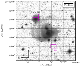
Figure 1: Red band image of HCG 91a, c and d from DSS-2. The purple rectangles denote the footprint of our WiFeS observations of HCG 91c. The location of the sky field was chosen to avoid any of the faint and extended tidal structures stemming from HCG 91a, including the faint tidal arm extending (on-sky) from HCG 91a to HCG 91c.

The data was acquired over two nights on 2012 August 15 and 16, with a seeing of 1.2-1.5 arcsec. Each individual science field of 25$\times$38 arcsec² was observed 4$\times$1400s, resulting in 5600s on-source per field. A blank patch of sky to the South-West of HCG 91a was observed for a total integration time of 700s between every pair of consecutive science frames.

WiFeS is a dual-beam integral field spectrograph with independent red and blue channels. We used the B3000 grating for the blue arm and the R7000 grating for the red arm, in conjunction with the RT560 dichroic. This setup allows us to have a complete wavelength coverage from 3800Å to 7000Å, as well as a high spectral resolution observation of the H$\alpha$ emission line to perform a detailed kinematic analysis. It is important to note here that with this instrumental setting, the final spectra associated with each spectral pixel (a.k.a spaxel) in the mosaic has a dual spectral resolution of R=3000 from 3800Å to 5560Å and R=7000 from 5560Å to 7000Å, corresponding to a full width at half maximum (FWHM) for emission lines of $\sim$100 km s^-1 and $\sim$43 km s^-1, respectively.

2.1.2 Data reduction

Each science exposure was individually bias subtracted, flat fielded, sky subtracted, wavelength and flux calibrated, as well as atmospheric refraction corrected with pywifes (v0.5.6), the new official python data reduction pipeline for WiFeS observations (Childress et al., 2014a, b). This new pipeline entirely replaces the now obsolete iraf pipeline (Dopita et al., 2010) by providing several key improvements: scriptability, reproducibility, advanced wavelength calibration technique using an accurate model of the instrument’s optics, multicore processing and compatibility with the first & second generations of CCD detectors in the WiFeS cameras. The pipeline is described in detail in Childress et al. (2014b), to which we refer the reader for more details about the different functions.

The reduced eight red science frames and eight blue science frames are median combined in two mosaics (red and blue) using a custom made python script. Because the wavelength sampling was chosen to be the same during the data reduction process, mosaicking only requires a shift of the data cubes in the spatial x- and y- directions. Given the seeing conditions and the WiFeS spaxel size of 1$\times$1 arcsec², we restrict ourselves to integer spatial shifts. The final mosaic contains 38$\times$50=1900 spaxels. Once the red and blue mosaics are constructed, we correct them for Galactic extinction using the Schlafly & Finkbeiner (2011) recalibration of the Schlegel et al. (1998) extinction map based on dust emission measured by COBE/DIRBE and IRAS/ISSA. We assume for HCG 91c a Galactic extinction A_V=0.052, following the NASA/IPAC Extragalactic Database (NED). The recalibration assumes a Fitzpatrick (1999) reddening law with $R_{V}$=3.1 and a different source spectrum than that used by Schlegel et al. (1998).

We note that the far blue end of a WiFeS spectrum below 4000Å (with the B3000 grating) is a known problematic region. The core reason, aside of a drop of the overall instrument transmission, is that the available flat-field lamps (at the epoch of our observations) have almost no flux at these wavelengths. It is therefore virtually impossible to accurately flat-field the data below 4000Å with the B3000 grating. pywifes combines lamp flat-field images with twilight sky flat-field images which mitigate this issue partially, but not entirely. In the present case, this flat-fielding issue directly affects the [O II] flux, to which we find a correction factor of 1.5 ought to be applied. This correction factor is only an average for the entire field of view, so that we decided not to rely on the [O II] line flux in our spaxel-based analysis of HCG 91c.

2.1.3 Spectral fitting

We fit the strong emission lines for all 1900 spaxels in our mosaic after fitting and removing the underlying stellar continuum in the spectra. This task is performed automatically using the custom build lzifu v0.3.1 idl routine, written by I-Ting Ho at the University of Hawaii (Ho et al., 2014, Ho et al., in prep.). lzifu is a modified version of the uhspecfit idl routine to which D.S.N. Rupke, J.A. Rich and H.J. Zahid all contributed. The code is a wrapper around ppxf (Cappellari & Emsellem, 2004), used to perform the continuum fitting, and mpfit (Markwardt, 2009), used to fit the emission lines with different gaussian components.

The lzifu routine first performs (via ppxf) the continuum fitting by looking at spectral regions free of emission lines. We refer the reader to the ppxf documentation for further details. We use the González Delgado et al. (2005) set of stellar templates with the Geneva isochrones to construct the best-matched stellar continuum for each spaxel. We note that we tested using the stellar templates based on the Padova isochrones instead, but found no significant difference in the fit results.

lzifu offers the possibility to fit one or multiple gaussian components to multiple emission lines simultaneously. In the present case, a visual inspection of the data revealed a very narrow structure of the different emission lines with no evidence of multiple peaks in any spaxel. For consistency, we performed two distinct fits of the emission lines - with one, and subsequently with two gaussian components. We detected the presence of a broadened base around the H$\alpha$ emission line in the $\sim$100 brightest spaxels, and confirmed the detection with a statistical f-test (e.g. Westmoquette et al., 2007). We performed this test blindly for the [N II] and H$\alpha$ emission lines only for all spaxels, and with a null-hypothesis rejection probability of 0.01. However, because a) the broadened base is visually only marginally detected around the H$\alpha$ line in $\sim 10$ out of 1081 spaxels with signal-to-noise (S/N) larger than 5, b) it is not detected around any other emission line, and c) beam-smearing effects may be responsible for some of the broad component, we choose to enforce a 1-gaussian component fit for every spaxel in our mosaic of HCG 91c.

We note here that nowhere in our observations do we detect clear multiple peaks in the emission line profile of H$\alpha$ as reported by Amram et al. (2003) in their Fabry-Perot observations of HCG 91c. Although the spectral sampling (0.35Å) and spectral resolution (R=9375 at H$\alpha$) of their data are slightly better than ours (0.44Å and R=7000), WiFeS (of which the instrumental design minimizes scattered light and other instrumental artefacts) should have clearly detected the distinct velocity components offset by $\sim$100 km s^-1 observed by Amram et al. (2003). A detailed comparison of the WiFeS line profile with the velocity structures of Amram et al. (2003) is presented in Appendix A. With no evidence for multiple components and/or significant asymmetries in the line profiles in our WiFeS observations, we are led to conclude that the gas in HCG 91c is associated to a single kinematic structure at all locations.

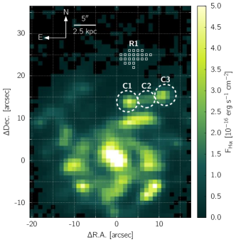
Figure 2: H$\alpha$ flux map of HCG 91c, before correcting the extragalactic reddening. The core of the galaxy and the spiral structure is traced by enhanced H$\alpha$ emission. Three star forming regions of interest “C1”, “C2” and “C3” are labelled accordingly. The region “R1” is also indicated, along with the individual spaxels it comprises. The x and y axis are in arcsec ($\equiv$ spaxels), centered on the brightest spaxel in H$\alpha$. At the distance of HCG 91c, 1 arcsec $\approx$ 503 pc.

The H$\alpha$ flux map of HCG 91c observed by WiFeS is shown in Figure 2 in units of $10^{-16}$ erg s^-1 cm^-2. The final emission line widths quoted in this article are corrected for the instrumental resolution.

Throughout this article, we analyze our WiFeS dataset on a per-spaxel basis to keep a high spatial resolution even at large distances from the galaxy center. To ensure trustworthy results, we adopt varying S/N cuts throughout our analysis. For example, we require S/N(H$\alpha$;H$\beta$)$\geq$5 to perform the extragalactic reddening correction. The specific S/N cuts will be discussed individually for each case in the next Sections. For clarity, we also include the associated S/N cut and number of spaxel in all relevant diagrams throughout this article.

A series of spaxels with S/N(H$\alpha$)$\geq$5 and S/N(H$\beta$)$<$5 are detected to the North of HCG 91c at the mean position [4;25]. This is the most distant star forming region (from the galaxy center) detected with WiFeS, and as such it holds unique clues regarding the state of the ionized gas at large radii. To ensure a reliable extragalactic correction, we have summed all of the contiguous spaxels with S/N(H$\alpha$)$\geq$5 into a combined spectrum, which we refer to as the “R1” region. The individual R1 spaxels are marked with empty white squares in Figure 2. We also indicate the location of three star forming regions with anomalous abundance and kinematics offsets, the “C1”, “C2” and “C3” regions.

2.1.4 Extragalactic reddening

We correct our WiFeS observations for extragalactic reddening using the H$\alpha$/H$\beta$ line ratio. HCG 91c does not contain any active galactic nuclei (AGN) which could increase the intrinsic line ratio value $R_{\alpha\beta}$, and we therefore assume that $R_{\alpha\beta}$ = 2.86 as in a case B recombination ($n_{e}=100$ cm^-1; T=$10^{4}$ K, see Osterbrock, 1989). We follow the methodology described in details in the Appendix A of Vogt et al. (2013), and use the extinction curve from Fischera & Dopita (2005) with R${}_{V}^{A}$=4.5. The choice of this extinction curve, very similar to that of Calzetti et al. (2000), is motivated by the fact that Wijesinghe et al. (2011) showed that for galaxies in the GAMA survey (Driver et al., 2009), it provides self-consistent estimates of the star formation rates computed from the UV, H$\alpha$ and [O III]. The resulting V-band extinction A${}_{\text{V}}$ in magnitudes is shown in Figure 3. The extragalactic reddening (and correction) is only calculated (and applied) for the 530 spaxels with S/N(H$\alpha$;H$\beta$)$\geq$5, corresponding to a line intensity detection threshold of $\sim$2$\times$10^-17 erg s^-1 cm^-2 Å^-1.

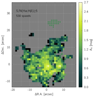
Figure 3: A${}_{\text{V}}$ extinction, calculated from the H$\alpha$/H$\beta$ emission line flux ratio. The center of the galaxy is the most affected by extragalactic reddening, with A${}_{\text{V}}>2$. Enhanced extinction regions are also associated with the spiral structure detected in Figure 2. The uncertainty in the A${}_{\text{V}}$ value is of the order of 0.6-0.8 for all spaxels.

The largest extinction is present towards the core of the galaxy with A${}_{\text{V}}>2$. Further out, the extinction drops to A${}_{\text{V}}$$\approx$1, with localized increases coherent with the spiral arms visible in Figure 2. Unlike most star forming regions in the spiral arms, we detect no enhancement of the extinction associated with the C1, C2 and C3 regions at the 1-sigma level (given an uncertainty of 0.6-0.8 in the A${}_{\text{V}}$ value).

2.2 VLA

The H I distribution in HCG 91 was observed with the Very Large Array (VLA) under the program AV0285 (P.I.: L. Verdes-Montenegro) on 2005 October 5. The observations were carried-out in the VLA D-configuration with 3.25hr of on-source integration and dual polarization using two intermediate frequency (IF). The resulting total bandwidth of the datacube is 6.2 MHz ($\sim$1200 km s^-1) with a resolution of 97 kHz. The correlator was setup to cover the entire H I spectral linewidth with a velocity resolution of $\sim$21.6 km s^-1. The data was calibrated following the standard VLA calibration and imaging procedures using NRAO’s Astronomical Image Processing Software (AIPS). The final absolute uncertainty in the flux density scaling is $\sim$10 per cent. The synthesized beam of the reduced datacube is 74”$\times$47”, with a position angle of 4.83^∘ West-of-North (Borthakur et al., 2010).

2.3 Pan-STARRS

HCG 91c was observed at multiple epochs with the Pan-STARRS 1 (PS1) telescope (Kaiser et al., 2002; Kaiser, 2004; Kaiser et al., 2010; Hodapp et al., 2004) on Haleakala (Maui) as part of the PS1 3$\pi$ survey (Chambers et al., in preparation). This survey mapped (several times) the entire sky visible from Hawaii ($\delta$$>$-30^∘) in five broad filters (g_P1:$\sim$400-550 nm; r_P1:$\sim$550-700 nm; i_P1: $\sim$690-820 nm; z_P1:$\sim$820-920 nm; y_P1:$\sim$920-1000 nm, see Tonry et al., 2012) between 2010 and 2014. The Pan-STARRS images presented in Section 4.1 were obtained from the online Postage Stamp server. These images were automatically processed by the PS1 Image processing Pipeline (IPP, see e.g. Magnier, 2007; Magnier et al., 2013). Specifically, the Pan-STARRS images presented in this article (see Figure 7) have been obtained from the 3$\pi$ survey processing version 2 (PV2) release. They have a pixel size of 0.25 arcsec, and are the result of the combination of 20 single epoch exposures obtained under natural seeing conditions ($\sim$1 arcsec).

3 The group-wide H I distribution in HCG 91

H I is an excellent tracer of past and ongoing gravitational interactions. For compact groups, H I can also be used to estimate the evolutionary stage of the group overall (Verdes-Montenegro et al., 2001). The H I map for HCG 91 obtained with the VLA is shown in Figure 4. The left and right panels show Position-Position and Position-Velocity projections of the data cube, respectively. Iso-intensity surfaces are fitted to the distribution of H I emission in the 3-dimensional datacube using the mayavi module in python (Ramachandran & Varoquaux, 2011), before being projected onto the respective 2-dimensional planes. Each iso-intensity level is shown with an 80 per cent transparency, with exception to the inner-most one with 0 per cent transparency. The locations of the HCG 91a, b, c and d galaxies are marked with black crosses. The location of the C1, C2 and C3 star forming regions in HCG 91c is indicated with small golden cubes and black crosses. H I structures of interest (see below) are marked with red-crosses for rapid identification. A large H I tail associated with HCG 91a is traced with a red rod. Figure 4 is also interactive, following a concept described by Barnes & Fluke (2008). By clicking on it in Adobe Acrobat Reader v9.0 or above, it is possible to load an interactive view of the (X;Y;v) data cube. The interactive model is also accessible via a supplementary HTML file compatible with most mainstream web browsers . When inspecting this interactive 3-D map, one should remember that it is not “fully” spatial, but rather an X-Y-v volume. Presenting the VLA 3-D data cube as 3-D model is similar to the example provided by Kent (2013), although our respective 3-D model creation methods are different (i.e. we do not use blender). The total H I mass associated with HCG 91 is 2.3$\times$10¹⁰M_⊙ (Borthakur et al., 2010).

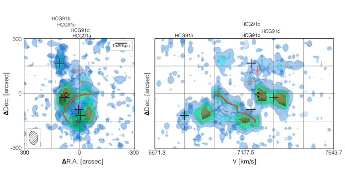
Figure 4: Position-Position (left) and Position-Velocity (right) projection of the H I gas content of HCG 91, as seen by the VLA. The gas density is traced by a series of iso-intensity semi-transparent surfaces (set at 1.3, 2.5, 3.5 and 6.0 mJy/beam, respectively). The location of the different group members is marked with black crosses, and labelled accordingly above either panels. Two H I clumps associated with the main gas reserve around HCG 91c are marked with red crosses for unambiguous identification. The large tidal tail originating to the South-East of HCG 91a is traced by a red rod. The C1, C2 and C3 star forming regions in HCG 91c are marked with golden cubes and black crosses (the golden cubes are 5 arcsec $\times$ 5 arcsec $\times$ 5 km s^-1 in size). The corresponding VLA beam size (74”$\times$47”, see Borthakur et al., 2010) is shown to the bottom left of the left panel. An interactive version of this Figure can be accessed either with Adobe Acrobat Reader v.9.0 or above by clicking on this Figure, or via most mainstream web browsers by opening the corresponding HTML file included as supplementary material to this article. The 3-D cube can be freely rotated and/or zoomed in and out. In the interactive cube, the blue axis is the velocity dimension, the red axis is the R.A. direction, and the green axis the Dec. direction. A series of pre-set views allow the viewer to easily reproduce projections of interest or remove the lowest intensity iso-surface for a clearer view of each galaxy. The golden cubes marking the location and spatial/kinematic extent of the C1, C2 and C3 star forming regions are best seen in the interactive counterpart of this Figure. NdlA: the interactive component of this Figure has been disabled in the arXiv version of the article (its compilation requires the media9 package, while arXiv currently only supports the obsolete movie15 package). The interactive Figure will be accessible from the final article in MNRAS (both as an interactive PDF inside the article itself, and as a supplementary interactive HTML document). Until then, readers can access the interactive HTML version of this Figure at http://www.mso.anu.edu.au/~fvogt/website/misc.html.

For ease of visualisation, we show in Figure 5 the different symbols marking the position of the galaxies, H I clumps of interest and tidal arm introduced in Figure 4 on top of a DSS-2 red band image, along with our WiFeS observation fields. The full extent of the different H I structures is traced with iso-contours (at a level of 2.5 mJy/beam and colored as a function of the gas velocity) in Figure 6.

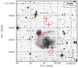
Figure 5: Red band image of HCG 91a,b,c and d from DSS-2. The image spans the same area as the Position-Position velocity diagram of Figure 4 (left), of which the same markers are shown for comparison. The purple rectangles denote the footprint of our WiFeS observations of HCG 91c.

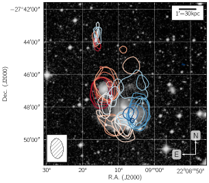
Figure 6: Red band image of HCG 91a,b,c and d from DSS-2. The image spans the same area as shown in Figure 4 (left) and 5. Iso-intensity contours trace the H I content of the group, and are color-coded as a function of their radial velocity, ranging from 6822.0 km s^-1 (dark blue) to 7405.5 km s^-1 (dark red), in steps of $\sim$21.6 km s^-1. The contours are extracted from the different velocity slices of the VLA datacube and trace an intensity of 2.5 mJy/beam.

Globally, the different sub-structures of the H I gas distribution in the group can be associated with the different individual galaxies. Specifically:

• HCG 91a: Spatially, this galaxy is coherent with the large H I structure to the South of the group. The large tidal feature detected in H I is also spatially coherent with a faint optical counterpart distinguishable in the red band DSS-2 image of the area (see Figure 5). Kinematically however, we find a mismatch of $\sim$220 km s^-1 between the optical redshift of the galaxy (6832 km s^-1, see Hickson et al., 1992) and the mean redshift of the H I structure. Although the optical redshift of HCG 91a associates the galaxy with a local H I over-density in the Position-Velocity diagram of Figure 4, most of the H I gas spatially-coherent with the galaxy (including the base of the tidal tail) is redshifted by up to $\sim$400 km s^-1 with respect to the optical redshift. The H I distribution observed with the VLA (both the spatial extent and the dynamic range of the different structures) is consistent with similar observations from Barnes & Webster (2001) using the Australia Telescope Compact Array (ATCA), while the optical redshift measurement of HCG 91a from Hickson et al. (1992) (z=0.022789) is consistent with the redshift measurement from the 6dF Galaxy Survey data release 3 (z=0.022739, see Jones et al., 2004, 2009) and with our own observations of the galaxy with WiFeS. Altogether, these observations confirm that the observed optical-radio redshift mismatch of HCG 91a is real. Here, we merely mention the existence of this redshift mismatch, and defer any further discussion to a later paper dedicated to our WiFeS observations of HCG 91a.

• HCG 91b: A spatially compact and kinematically extended ($\sim$490 km s^-1) H I structure is associated with this galaxy. The large range of the H I kinematics is consistent with the fact that HCG 91b is seen almost edge-on on.

• HCG 91c: A rotating H I disk with a velocity range of $\sim$200 km s^-1 ($\sim$7200-7400 km s^-1) is associated both spatially and kinematically with the optical counterpart of HCG 91c. We find a small kinematic offset of $\sim$10 km s^-1 between the optical redshift of HCG 91c measured by Hickson et al. (1992) and the mean velocity of the H I structure. The largely undisturbed morphology of the H I distribution is suggesting the presence of only minimal tidal effects for this galaxy. To the North-West, two fainter H I sub-structures (marked with red crosses in Figure 4) appear connected to the main gas reservoir of HCG 91c. They are also connected (less strongly) at the 1.3 mJy/beam level to the H I structure associated with HCG 91b. These two H I clumps are located 116 arcsec $\approx$ 58.4 kpc and 150 arcsec $\approx$ 75.5 kpc from the center of HCG 91c. They have no visible optical counterpart in the DSS-2 red band image in Figure 5. Spatially, HCG 91c is located $\sim$15 kpc to the North-East of the large tidal arm originating from HCG 91a. The H I gas in the tidal arm is blueshifted by 150-250 km s^-1 from the mean velocity of HCG 91c.

• HCG 91d: This galaxy is not associated with any H I structure kinematically.

The large tidal feature originating from HCG 91a makes the HCG 91 compact group a Phase 2 group in the classification of Verdes-Montenegro et al. (2001), although some of the H I gas is still clearly associated with the galaxies HCG 91b and HCG 91c. The H I reservoir associated with HCG 91c appears largely undisturbed from a kinematic point of view. The two H I gas clumps located to the North-West of HCG 91c may have resulted from tidal stripping, suggesting that HCG 91c is experiencing the first stages of tidal disruption via gravitational interaction. The H I bridge at the 1.3 mJy/beam level connecting the gas reservoir of HCG 91b and HCG 91c could be seen as evidence for an ongoing interaction between the H I envelopes of these two galaxies, although the exact bridge structure would require a higher spatial sampling to be clearly established.

4 The galaxy HCG 91c

Here, we describe the different characteristics of HCG 91c as seen by WiFeS and Pan-STARRS. We focus our analysis on the strong emission lines and the associated underlying physical characteristics of the ionized gas. We restrict ourselves to a description of the system, and postpone a global discussion of the different measurements until Section 5.

4.1 Spatial distribution of the stellar light

A color-composite image of HCG 91c, constructed from the Pan-STARRS i_P1, r_P1 and g_P1 band images, is shown in Fig. 7. The same image is shown twice, with the intensity stretch adjusted to reveal the outer regions (left panel) and the inner spiral structure (right panel) of HCG 91c. The WiFeS mosaic footprint is traced by a dashed rectangle in the left panel, and the location of R₂₅ is traced by an ellipse in the right panel. Specifically, R₂₅=26.75$\pm$3.25 arcsec =13.5$\pm$0.2 kpc with an ellipticity of 0.91, following NED and the Third Reference Catalogue of Bright Galaxies (de Vaucouleurs et al., 1991). We note that this value is consistent with the estimate of R₂₅=28.45 arcsec and an ellipticity of 0.87 from the Surface Photometry Catalogue of the ESO-Uppsala Galaxies (Lauberts & Valentijn, 1989).

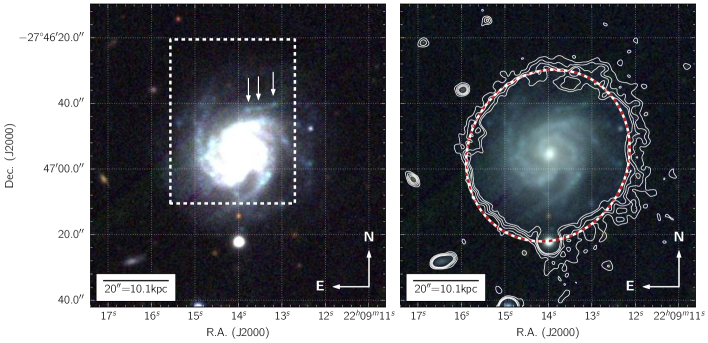
Figure 7: Color combination of Pan-STARRS i_P1, r_P1 and g_P1 images (shown as the red, green and blue channels respectively) of HCG 91c. The color scheme is stretched to reveal the galaxy outskirts (left) or the inner region and spiral structure (right). The WiFeS observations footprint is marked with a dashed rectangle in the left panel, along with three arrows marking the location of the C1, C2 and C3 regions. R₂₅ is traced by the dashed ellipse in the right panel. Also in the right panel, low level iso-contours constructed from a gaussian smoothed g_P1 band image highlight the full optical extent of HCG 91c on the sky at a distance of $\sim$R₂₅.

HCG 91c harbors a regular, tightly wrapped spiral pattern with a bright nucleus. The outer limit of the stellar disk, traced by white iso-contours in the right panel of Fig. 7 (extracted from the g_P1 image) is mostly regular, with the brightness dropping the most sharply towards the SE. The spiral arms are extending (at least) 20 arcsec $\approx$ 10 kpc from the galaxy center, but their brightness decreases rapidly beyond $\sim$5 kpc.

The C1, C2 and C3 regions defined in Figure 2 appear as three distinct compact features (each indicated by a white arrow in the left panel of Figure 7 for clarity). The Pan-STARRS broad-band images primarily trace the stellar content of HCG 91c, and one must use caution when comparing this view to that of the ionized gas provided by WiFeS. Nevertheless, with a diameter of $\sim 6$ Pan-STARRS pixels $\approx$ 1.5 arcsec $\approx$ 750 pc across, it is very likely that the optical emission associated with the C1, C2 and C3 star forming regions is unresolved both in our WiFeS observations and in the Pan-STARRS image of HCG 91c.

4.2 Emission line maps and line ratio diagrams

We present the flux line maps for the principle optical emission lines ([O II], H$\beta$, [O III], H$\alpha$, [N II], [S II]) in the spectrum of HCG 91c (before applying the extragalactic reddening correction) in Figure 8. For comparison purposes, all the maps are shown with the same color stretch and cuts. In each panel, the white contours at 2.2$\times$10^-17 erg s^-1 cm^-2 trace approximatively the regions with S/N$\geq$5.

The structure of the emission from the [N II] and [S II] lines is similar to H$\alpha$, although with an overall weaker intensity. There is a distinct lack of [O II] emission from the core of the galaxy, a region subject to a larger reddening (see Figure 3). The noise level is much higher in the [O II] map, because the lines are located at the very blue end of the WiFeS spectra (in a region subject to flat-fielding problems, see Section 2.1.2). The spatial distribution of the [O III] line is distinctly different from that of H$\alpha$. The lack of emission at the core of the galaxy is reminiscent of [O II], and is consistent both with a larger extinction and with a higher gas metallicity overall in the core of HCG 91c (see Section 4.3). Further out, the [O III] emission is the strongest in the C1 and C3 regions. By comparison, the H$\alpha$ emission associated with the C1 and C3 regions is at a level comparable to other star forming regions within the spiral arms.

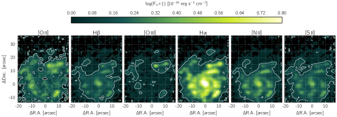
Figure 8: Maps for the different emission lines considered in this article, shown with a uniform color scheme and color stretch for comparison purposes. For each line, the white contours at 2.2$\times$10^-17 erg s^-1 cm^-2 approximatively trace the regions with S/N$\geq$5.

The standard line ratio diagrams $\log$ [N II]/H$\alpha$ vs $\log$ [O III]/H$\beta$ and $\log$ [S II]/H$\alpha$ vs $\log$ [O III]/H$\beta$ for HCG 91c are shown in Figure 9. Each 353 spaxels for which S/N(H$\alpha$;H$\beta$)$\geq$5 and S/N([O III];[N II];[S II])$\geq$2 are shown as individual squares, color-coded as a function of S/N([O III]). The first S/N selection condition results from the extragalactic reddening correction described previously. A lower S/N cut for [O III], [N II] and [S II] is then acceptable given that both H$\alpha$ and H$\beta$ are clearly detected and strongly constrain the velocity and velocity dispersion of all the different emission lines. The color scheme choice reflects the fact that S/N([O III])$\geq 2$ is in all cases the limiting condition. The grey error bars shown in each diagram indicate the 1-sigma error associated with the line ratio measurements, calculated from the errors measured by lzifu based on the variance measurements propagated through the pywifes data reduction pipeline.

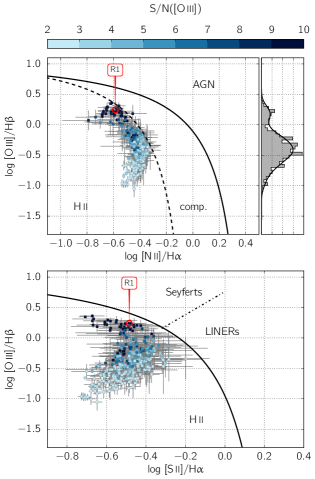
Figure 9: Standard line ratio diagnostic diagrams $\log$ [N II]/H$\alpha$ vs. $\log$ [O III]/H$\beta$ (top) and $\log$ [S II]/H$\alpha$ vs. $\log$ [O III]/H$\beta$ (bottom). Each spaxel with S/N(H$\alpha$;H$\beta$)$\geq$5 and S/N([O III];[N II];[S II])$\geq$2 are marked with squares colored as a function of S/N([O III]). The position of the R1 integrated spectra is marked with a red circle and labelled accordingly. The 1-sigma errors are shown in grey for each measurement. The full black lines are the maximum starburst diagnostic lines from Kewley et al. (2001), the dashed line is the starburst diagnostic line from Kauffmann et al. (2003), while the Seyferts-LINERs separation from Kewley et al. (2006) is marked as a dash-dotted line in the bottom panel. The histogram in the upper panel shows the spaxel distribution as a function of $\log$ [O III]/H$\beta$, while the smooth distribution (traced by the black curve) was derived by performing a Kernel Density Estimation on the distribution of $\log$ [O III]/H$\beta$ values.

Within the errors, the different spaxels form a well defined sequence in both line ratio diagrams, extending 1.5dex along the $\log$ [O III]/H$\beta$ direction. The spaxel density along the sequence is continuous, except for a marked decrease at $\log$ [O III]/H$\beta$$\approx$0. This gap, best seen in the density histogram in the right-hand side of the upper panel of Figure 9, is most certainly not a consequence of low S/N measurements. Indeed, spaxels on either side and across this gap in the distribution have strong oxygen emission with S/N([O III]$\ga$6, and are therefore clearly detected.

In Figure 10, we show the $\log$ [O III]/H$\beta$ line ratio map for all 353 spaxels visible in either panel of Figure 9. Along with the R1 region, the spaxels associated with the C1, C2 and C3 regions have $\log$ [O III]/H$\beta$$\geq$0. They are forming the upper end of the star forming sequence visible in the line ratio diagrams. Altogether, Figures 9 and 10 indicate an abrupt change in the physical conditions of the ionized gas between the C1, C2 and C3 regions and their immediate surroundings.

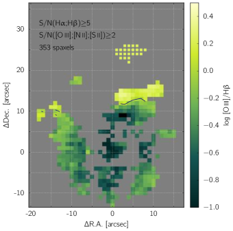
Figure 10: Map of $\log$ [O III]/H$\beta$ for spaxels with S/N(H$\alpha$;H$\beta$)$\geq$5 and S/N([O III];[N II];[S II])$\geq$2. Most spaxels with a positive ratio are located in the C1, C2 and C3 regions. The black line traces the iso-contour corresponding to $\log$ [O III]/H$\beta$=0.

4.3 Oxygen abundance and ionization parameters

We now delve deeper into the physics of emission line ratios, and compute oxygen-abundances and ionization parameters for each 353 spaxels with S/N(H$\alpha$;H$\beta$)$\geq$5 and S/N([O III];[N II];[S II])$\geq$2. The concept and the method employed here follow Dopita et al. (2013a). We use the pyqz v0.6.0 python module to compute, for each spaxel, the value of the oxygen abundance 12+$\log$(O/H) and the ionization parameter $\log$(q) (with q in cm s^-1). The code relies on a series of grids of photoionization models computed with mappings iv - the most recent embodiment of the mappings code (Dopita et al., 1982; Binette et al., 1982; Binette et al., 1985; Sutherland & Dopita, 1993; Groves et al., 2004; Allen et al., 2008) - which for a distinct set of line ratio diagrams allow to disentangle the values of 12+$\log$(O/H) and $\log$(q) over a large parameter space ($5-0.05~{}Z_{\odot}$ and $6.5\leq\log(\mathrm{q})\leq 8.5$). Among other updates, mappings iv allows for a non-Maxwellian distribution for the electron energies in the form of a $\kappa$-distribution (Nicholls et al., 2012, 2013; Dopita et al., 2013b). Here, we adopt $\kappa$=20, but we note that this choice does not significantly affect our analysis, given the limited influence of a $\kappa$ distribution on the intensity of strong emission lines.

We note that for this work we have upgraded pyqz from v0.4.0 publicly released by Dopita et al. (2013b) to v0.6.0. In this latest version, pyqz can fully propagate errors in the line flux measurements through to the estimation of the abundance and ionization parameters (but still relies on the same mappings iv models of Dopita et al., 2013b). The new pyqz v0.6.0 will be publicly released in the near future along with updated mappings iv models (Sutherland et al., in prep.), and is available on-demand until then. For completeness, we describe in Appendix B how observational errors are propagated in this new version of pyqz and how the final 1-sigma uncertainty level on the 12+$\log$(O/H) and $\log$(q) values is computed, namely via the propagation of the full probability density function associated with each emission line measurement.

In total, eight diagnostic grids are available in pyqz to compute the abundance and ionization parameter of a given spectrum. In principle, each of these grids can provide an estimate of 12+$\log$(O/H) and $\log$(q), which can then be combined to provide a global estimate. In practice, and for the present case, we only used the diagnostics not involving [O II] because these emission lines are subject to flat-fielding issues (see Section 2.1.2). In addition, an inherent twist in the model grid over the region of interest for HCG 91c renders the diagram $\log$ $[$N II$]$/H$\alpha$ vs $\log$ [O III]/H$\beta$ unusable in the present case. Ultimately, we are left with just two suitable diagnostic grids: $\log$ $[$N II$]$/[S II] vs $\log$ [O III]/H$\beta$ and $\log$ $[$N II$]$/[S II] vs $\log$ [O III]/[S II].

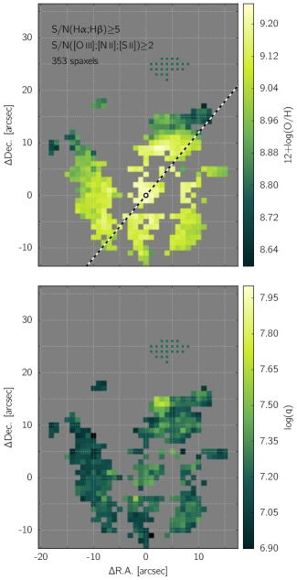
Figure 11: Gas phase oxygen abundance (top) and ionization parameter (bottom) measured with the pyqz python module for all spaxels with S/N(H$\alpha$;H$\beta$)$\geq$5 and S/N([O III];[N II];[S II])$\geq$2. In the top panel, the dashed line traces the major axis of HCG 91c with a P.A. of 40 degrees West-of-North (see Section 4.4).

The resulting 12+$\log$(O/H) and $\log$(q) maps for HCG 91c are shown in Figure 11. As mentioned previously, the overall decrease of the [O III] flux in the inner regions of HCG 91c is associated with increasing oxygen abundances. The peak oxygen abundance at the galaxy center is 12+$\log$(O/H)$\approx$9.25. By comparison, the oxygen abundance of the R1 region is found to be 12+$\log$(O/H)$\approx$8.80. The oxygen abundance of the C1, C2 and C3 regions is of the order of 8.7-8.9. The ionization parameter map is uniform throughout the entire galaxy ($7.10\la\log(\mathrm{q})\la 7.35$). The C1 region is a notable and the only significant departure from the mean with $\log$(q)$\approx$7.65.

In Figure 12, we construct the abundance gradient of HCG 91c as a function of the deprojected radius. Every 353 spaxels for which we derived an oxygen abundance are shown individually. The vertical error bar associated to each measurement corresponds to the error computed by pyqz v0.6.0. To deproject the position of each spaxel in the disk of HCG 91c, we assume an ellipticity $b/a$=0.8$\pm$0.08 (measured manually from the r_P1 image of HCG 91c from Pan-STARRS), and a position angle P.A.=40^∘ West-of-North (measured from the rotation map of HCG 91c, see Section 4.4). This P.A. is in disagreement with the P.A. available in NED based on near-IR images from 2MASS (Skrutskie et al., 2006) of 5^∘ West-of-North, but is in good agreement with the P.A. derived from optical images from the Surface Photometry Catalogue of the ESO-Uppsala Galaxies (Lauberts & Valentijn, 1989) of 46^∘ West-of-North. The horizontal error bar associated with each measurement correspond to an estimated 10 per cent measurement error on the ellipticity. We assumed the center of the galaxy to be located at the position [0,0], coincident with the peak H$\alpha$ emission, which given the seeing conditions is also consistent with the kinematic center of the galaxy, as described in the next Section.

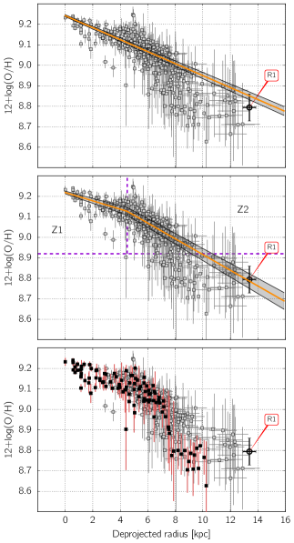
Figure 12: Oxygen abundance gradient in HCG 91c. Each 353 spaxels for which 12+$\log$(O/H) could be measured (see Figure 11) are shown individually with their associated 1-sigma errors. The galaxy center, taken to be the peak of the H$\alpha$ emission line flux map, is at the position [0,0] (see Figure 2). A position angle P.A. = 40^∘ and an ellipticity $b/a$=0.8 are assumed to deproject the radius of each spaxel within the disk of HCG 91c. The horizontal error bars correspond to a measurement error of 10 per cent of the ellipticity. The vertical error bars are the error computed by pyqz v0.6.0. The linear best fit (and associated 1-sigma error) to all the spaxels is shown in the top panel. A broken linear fit, better matching the outer regions of the galaxy, is shown in the middle panel. In the bottom panel, the spaxels located within 3 arcsec from the galaxy’s major axis (shown in Figure 11) are drawn in black with their associated errors in red. They reveal the abrupt drop of $\sim$0.2 dex in oxygen abundance at $\sim$7.5 kpc to the North-West of the galaxy center: the location of the C1, C2 and C3 star forming regions.

As illustrated in the top panel of Figure 12, a linear fit to the full set of data points fails to properly match the outer regions of the disk. It is clear from Figure 11 that our sampling of the outer regions of the disk (where 12+$\log$(O/H)$\leq$8.92) is poor, and largely composed of the C1, C2 and C3 regions. Hence, the global gradient fit is largely influenced by the spaxels in the inner regions of HCG 91c. In the middle panel of Figure 12, we use a linear broken fit to better reproduce the trend in the oxygen abundance throughout HCG91c. The fit is broken at 4.5 kpc from the galaxy center - the approximate radius at which the oxygen abundance gradient appears to steepen. An inner gradient is derived from spaxels in the Zone 1 (Z1; radius$<$4.5kpc, 12+$\log$(O/H)$>$8.92), while an outer gradient is derived from spaxels in the Zone 2 (Z2; radius$\geq$4.5kpc, 12+$\log$(O/H)$>$8.92), and forced to match the inner gradient at 4.5 kpc. The respective slopes of the different gradients are compiled in Table 2. All oxygen abundance gradients were derived using the Orthogonal Distance Regression routines inside the scipy module in python.

A series of spaxels beyond 7 kpc from the galaxy center remain below the best fit outer gradient by $\sim$0.15 dex. In the bottom panel of Figure 12, we show in black the spaxels located within 3 arcsec from the galaxy’s major axis visible in Figure 11. These spaxels trace an abrupt drop in the oxygen abundance of $\sim$0.2 dex at 7 kpc from the galaxy center over a distance of 1 kpc = 2 WiFeS spaxels. This sharp oxygen abundance decrease is essentially unresolved (spatially) in our data set, so that its true nature (physical discontinuity in the oxygen abundance or sharp but continuous decrease) remains uncertain. It is however clear that the intensity of the oxygen abundance drop at 7 kpc is inconsistent with any linear gradient extrapolated from the inner regions of HCG 91c.

We deliberately use only spaxels in the zone Z2 to derive the best-fit linear outer gradient, as we detect spaxels with 12+$\log$(O/H)$>$8.92 for (almost) all azimuths beyond a radius of 4.5 kpc. Our sampling of less enriched gas is much less uniform, so that including all the spaxels with 12+$\log$(O/H)$<$8.92 in the outer gradient fit would wrongly bias it towards the C1, C2 and C3 regions of which the abundances (as illustrated in the bottom panel of Figure 12) are clearly inconsistent with a linear gradient. Although the outer gradient is derived solely from the Z2 spaxels, we note that its slope nevertheless matches some of the outer regions of HCG 91c, including the R1 region.

Table 2: Characteristics of the different oxygen abundance gradients presented in Figure 12.

Gradient	Fitted region(s)	Slope	Zero point
		[dex kpc-1]
global fit	all	-0.029$\pm$0.001	9.242$\pm$0.005
inner fit	Z1	-0.020$\pm$0.003	9.219$\pm$0.007
outer fit	Z2	-0.038$\pm$0.002	9.300$\pm$0.011

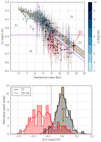
Figure 13: Top: same as the middle panel of Figure 12, but with the individual spaxels colored as a function of S/N([O III]). The diagram is divided in four gradient zones (labelled Z1 to Z4) based on the overall trend morphology. For clarity, errors for spaxels with S/N([O III])$\geq$9 are shown with thicker dark-red lines. Bottom: histogram and associated smooth distribution of the oxygen abundance offset from the best-fit outer-gradient, for spaxels in the Z2 zone (black) and in the Z3+Z4 zones (red).

In the top panel of Figure 13, we color-code the different spaxels as a function of their associated S/N([O III]. Most spaxels lying in the Zone 4 (Z4; 12+$\log$(O/H)$<$8.92, 12+$\log$(O/H) more than 0.075 dex below the best fit outer gradient based on the Z2 spaxels) are clearly detected, and their errors (shown in dark red for clarity) place them 1-2 sigma below our best-fit outer gradient. Their offset in oxygen abundance is best seen in the Figure’s bottom panel, showing the distribution of oxygen abundances for all spaxels in the zones Z2 and Z3+Z4. While some spaxels below 12+$\log$(O/H)=8.92 are consistent with the linear gradient estimate based on the Z2 spaxels out to 13 kpc (i.e. spaxels in the zone Z3), most lie 0.15 - 0.3 dex lower (in the zone Z4).

Most spaxels in the zone Z4 belong to the C1,C2 and C3 regions, as illustrated in Figure 14. It can be noted that as the C1, C2 and C3 regions are located along or near the P.A. of HCG 91c, their deprojected radii are not subject to large uncertainties. The Z3 spaxels are on the other hand all located in the outer regions of the spiral arm extending Northward from the left-hand side of HCG 91c. Especially, the lack of S/N in the [-10;15] area (see Figure 11) appears consistent with the lack of detection of Z3 spaxels at a radius of 10-11 kpc.

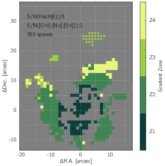
Figure 14: Spatial distribution of the spaxels in the different gradient zones Z1 to Z4 defined in Figure 13.

4.4 Kinematics of the ionized gas

In Figure 15, we show the ionized gas velocity map (center) and velocity dispersion (right) of HCG 91c. In the left panel, we show the H$\alpha$ intensity map overlaid with the iso-velocity contours. We use the freely available python routine fit_kinematic_pa from M. Cappellari to measure the P.A. of HCG 91c from its gas kinematics: P.A. = 40 $\pm$ 4 degrees West-of-North. This routine (originally written in idl) was used extensively by Cappellari et al. (2007) and Krajnović et al. (2011), and is described in Appendix C of Krajnović et al. (2006). The P.A.=40^∘ (black & white dashed line) direction and the galaxy center (white dot) used to construct the abundance gradient of HCG 91c shown in Figure 13 are shown in the left and middle panel of Figure 15 for completeness.

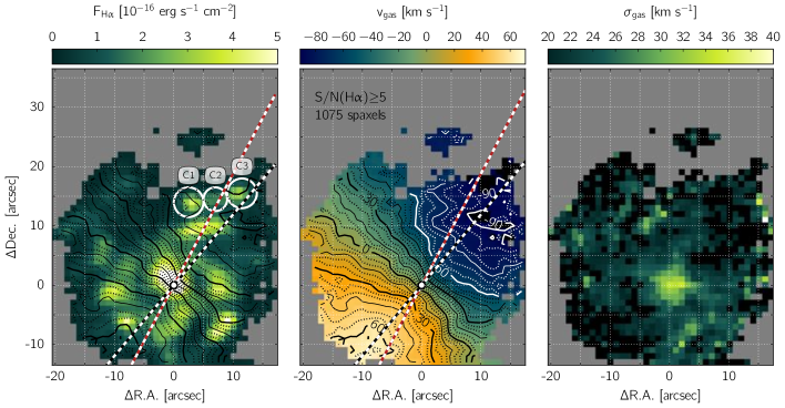
Figure 15: Velocity (center) and velocity dispersion (right) maps of HCG 91c, for all spaxels with S/N(H$\alpha$)$\geq$5. Iso-velocity contours are shown in the middle panel, and are also overlaid over the H$\alpha$ flux map of HCG 91c is the left panel. In the left and middle panel, the center of the galaxy (traced by the peak H$\alpha$ line flux) is marked with a white circle, and the black & white dashed line traces the principal axis of HCG 91c (P.A.=40^∘ West-of-North). The dark-red & white dashed line is rotated by 12^∘ counter-clockwise from the galaxy’s major axis, and is designed to pass through the C1-C2-C3 complex of star forming regions. The Position-Velocity diagrams in Figure 16 are extracted along these two directions. For the iso-velocity contours, the thick-full lines are spaced by 30 km s^-1, the thin-full lines are spaced by 15 km s^-1 and the dashed lines are spaced by 5 km s^-1.

The kinematic signature of the gas in HCG 91c is consistent with regular rotation. The quoted velocities assume a rest frame velocity of 7319 km s^-1 (z=0.024414; Hickson et al., 1992). We find an overall asymmetry between the redshifted and blueshifted sides that could be reconciled if the rest-frame velocity was reduced by 11 km s^-1 to 7308 km s^-1 (as measured by fit_kinematic_pa). This offset would also help reconcile the optical redshift of HCG 91c with the H I kinematic of the galaxy measured by the VLA (see Section 3).

The velocity dispersion of the ionized gas is throughout the entire disc of HCG 91c ranging from $\sim$20 km s^-1 to 40 km s^-1. Accounting for the thermal broadening of the lines ($\sigma_{\text{Th}}\approx 13(T/10^{4})^{0.5}$ km s^-1 for the Hydrogen lines, see Osterbrock, 1989), this corresponds to an intrinsic velocity dispersion range of $\sim$15-38 km s^-1. The largest velocity dispersions are found towards the galaxy center, and are most certainly influenced by beam smearing, given the seeing conditions during our observations (1.2-1.5 arcsec). No significant increase of the velocity dispersion is detected towards the C1, C2 and C3 clumps.

We detect some deviations from a regular rotation signature at and around the positions [5,15] to [12,12] - the location of the C1, C2 and C3 regions. Specifically, the C1, C2 and C3 regions are redshifted from (i.e. are lagging behind) the regular rotation of the galaxy by 5-10 km s^-1. We recall that the error associated with the spectral calibration of the red WiFeS datacube is of the order of 0.05Å (see Section 2.1.2 and Childress et al., 2014b) or 2.3 km s^-1 at H$\alpha$, so that a 5-10 km s^-1 offset corresponds to a 2-3 sigma detection. The fact that the kinematic distortion is extended and tracks the bright spaxels distribution of the C1, C2 and C3 regions suggest that the distortion is real, although a greater spectral resolution and finer spatial sampling would be beneficial to confirm its existence.

To further quantify the distortions of the velocity map of HCG 91c associated with the C1, C2 and C3 star forming regions, we construct two Position-Velocity (PV) diagrams. We choose the projection axis to be oriented a) along the galaxy’s P.A. and b) along an axis rotated by 12^∘ counter-clockwise from the galaxy’s major axis. In both cases, we set the zero-point at the galaxy center and add 11 km s^-1 to the measured velocities to correct the global kinematic asymmetry mentioned previously. The value of 12^∘ bears no special significance other than ensuring that the second axis passes through the C1-C2-C3 complex of star forming regions. The resulting PV diagrams are shown in Figure 16. Every spaxel within 3 arcsec and 1 arcsec (respectively) from the two projection axis and with S/N(H$\alpha$)$\geq$5 for which the line velocity can be measured accurately is shown as an individual red square (redshifted side of the galaxy) or a blue diamond (blueshifted side of the galaxy), as a function of its (projected) distance along the PV axis.

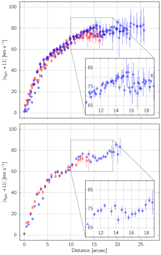
Figure 16: Top: Position-Velocity diagram of the velocity map shown in Figure 15, extracted along the axis passing through the galaxy center and with P.A. = 40^∘ West-of-North (shown with a black & white dashed line in Figure 15). Each spaxel within 3 arcsec of the axis and with S/N(H$\alpha$)$\geq$5 is shown as a red square (redshifted side of HCG 91c) or a blue diamond (blueshifted side of HCG 91c). A correction of 11 km s^-1 was added to the velocity of each spaxel to correct the global kinematic asymmetry detected in the velocity field. Bottom: idem, but for spaxels with S/N(H$\alpha$)$\geq$5 located within 1 arcsec from an axis rotated by 12^∘ counter-clockwise from the galaxy’s major axis (traced with a dark-red & white dashed line in Figure 15).

Along the major axis of the galaxy, after a linear increase out to $\sim$2 arcsec, the slope of rotation velocity decreases and remains consistent between the red- and blueshifted sides out to $\sim$12 arcsec. While the redshifted gas velocity flattens out at $\sim$75 km s^-1 beyond 12 arcsec, the blueshifted gas increases up to 80$\pm$3 km s^-1 beyond 22 arcsec. Assuming an ellipticity for HCG 91c of 0.8$\pm$0.08, we find the absolute rotation velocity of the gas at a radii greater than 11 kpc to be 100$\pm$11 km s^-1.

A noticeable feature of the top diagram is the kinematic behaviour of the blueshifted gas from 12 to 20  arcsec. As the magnified inset diagram in Figure 16 illustrates, two velocity “branches” separated by 5-10 km s^-1 at the 1-2 sigma level exist in this range. Especially, the “bottom” branch corresponds to spaxels in the C3 region, and is the signature of the lag of the C3 star forming region mentioned previously. The velocity lag of the C1, C2 and C3 complex of star forming regions is best seen in the bottom panel of Figure 16, in which the blue velocity curve decrease by $\sim$5-10 km s^-1 at 16 arcsec from the galaxy center (i.e. at the location of the C2 star forming region).

Spiral galaxies in compact groups have been observed to host a wide range of rotation signatures with sometimes large asymmetries and/or perturbations (see e.g. Rubin et al., 1991). As compact groups favor strong gravitational interactions between galaxies, the existence of small perturbations in the velocity field of HCG 91c (located inside a compact group) is in itself not surprising. Of interest however is the fact that the star forming regions with localized lower oxygen abundances are associated with localized kinematic anomalies. This abundance$\leftrightarrow$kinematic connection indicates that both the gas composition and motion in the C1, C2 and C3 star forming regions are inconsistent with their immediate surroundings.

4.5 Star formation rate

We can convert the H$\alpha$ line flux of each spaxel in our WiFeS mosaic (see Figure 2) into a star formation rate (SFR_Hα) following the recipe of Murphy et al. (2011) derived using starburst99 (Leitherer et al., 1999) and assuming a Kroupa (2001) initial mass function (IMF):

$$\mathrm{SFR}_{\mathrm{H}\alpha}=5.37\times 10^{-42}\frac{L_{\mathrm{H}\alpha}}{\mathrm{ergs}^{-1}},$$ (1)

where $L_{\mathrm{H}\alpha}$ is the total H$\alpha$ luminosity, derived from our measured de-reddened fluxes per spaxel and given the assumed distance to HCG 91c of 104 Mpc. This recipe results in a SFR 68 per cent of what would be derived using the Kennicutt (1998) formula, largely because of differences in the assumed IMF characteristics (Calzetti et al., 2007; Kennicutt & Evans, 2012). The resulting SFR map of HCG 91c is shown in Figure 17, where only the 530 spaxels with S/N(H$\alpha$; H$\beta$)$\geq$5 and the R1 region that were corrected for extragalactic reddening are shown. We note that our spatial resolution of 0.5 kpc arcsec^-1 is similar to the scale of the star forming complexes studied by Murphy et al. (2011), so that issues associated with using a “mean” H$\alpha$-to-SFR conversion factor on small scales does not apply in our case (see Murphy et al., 2011; Kennicutt & Evans, 2012).

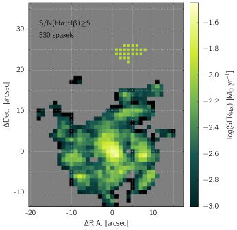
Figure 17: Star formation rate derived from the H$\alpha$ flux, for all spaxel corrected for extragalactic reddening. The galaxy center is the most active region, and the spiral structure is also visible. Localized enhancements of the star formation rate are detected in the C1, C2 and C3 regions.

As expected from the H$\alpha$ emission line map, star formation activity in HCG 91c is most intense in the central region of the galaxy, with additional hot spots along the spiral arms. The total SFR_Hα for HCG 91c (summed from all the spaxel with S/N(H$\alpha$; H$\beta$)$\geq$5 and the R1 region) is 2.10$\pm$0.06 M_⊙ yr^-1. This value is in excellent agreement with the estimated 2.19 M_⊙ yr^-1 from Bitsakis et al. (2014) based on a full SED fitting of the integrated light of HCG 91c.

Assuming a total stellar mass M_∗=1.86$\times 10^{10}$ M_⊙ for HCG 91c (Bitsakis et al., 2014), we obtain a specific star formation rate sSFR = 1.13$\pm$0.05$\times 10^{-10}$ yr^-1. This is comparable to the lowest sSFR measured by Tzanavaris et al. (2010) in 21 star forming HCG galaxies from their UV and IR colors, but well within the distribution of sSFR reported by Plauchu-Frayn et al. (2012) for $\sim$50 late-type galaxies (SBc and later) in compact groups using full optical spectrum fitting with stellar population synthesis models. In fact, HCG 91c is extremely consistent with the SFR vs M_∗ and sSFR vs M_∗ relations constructed from the SDSS and GAMA datasets for $z<0.1$ star forming galaxies by Lara-López et al. (2013). For reference, we list in Table 3 the different characteristics of the C1, C2 and C3 regions, whilst their integrated spectra are presented in Figure 18.

Table 3: Main integrated characteristics of the C1, C2 and C3 star forming regions

Region	C1	C2	C3
$<\Delta\mathrm{R.A.}>$ $[$ arcsec $]$	3.2	7.0	10.5
$<\Delta\mathrm{Dec.}>$ $[$ arcsec $]$	13.5	13.5	15.3
v ${}_{\text{gas}}$ (line of sight) $[$km s-1 $]$	7245$\pm$4	7236$\pm$3	7230$\pm$4
$\sigma_{\text{gas}}$ $[$km s-1 $]$	21$\pm$2	20$\pm$2	20$\pm$2
F(H$\alpha$) $[$10-16 erg s-1 cm${}^{-2}]$	64.0$\pm$8.9	23.8$\pm$6.0	49.6$\pm$9.0
SFRHα $[$10-2 M☉ yr-1$]$	4.4$\pm$0.6	1.7$\pm$0.4	3.4$\pm$0.6
LHα $[$1039 erg s-1$]$	2.1$\pm$0.3	0.8$\pm$0.2	1.6$\pm$0.3

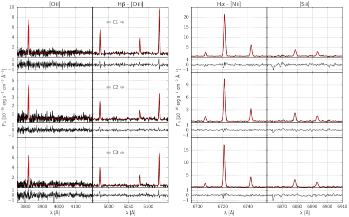
Figure 18: Raw integrated spectra (black) and lzifu fit (red) of the C1, C2 and C3 star forming regions. The dominant emission lines present in each panel are labelled on top of each column for clarity.

5 Discussion: the peculiar star forming regions of HCG 91c

By and large, HCG 91c appears as a rather unremarkable star forming spiral galaxy. It hosts regular star formation rates throughout its disc comparable to other similar galaxies in the field, and an overall regular rotation (as traced by the ionized gas). This galaxy also hosts a linear oxygen abundance gradient out to $\sim 4.5$ kpc, which then breaks to a steeper linear gradient. The H I gas distribution around the galaxy traced by the VLA is largely undisturbed. The cold dust contours measured by Herschel/SPIRE at 250 $\mu$m display a high degree of azimuthal symmetry (Bitsakis et al., 2014). Mendes de Oliveira et al. (2003) report that HCG 91c is an outlier with respect to the B-band Tully-Fisher relation, in that its absolute B-band magnitude M_B is 2 mag brighter than expected from its rotation velocity, and concluded (also based on the two distinct kinematic components reported by Amram et al., 2003) that HCG 91c may be the result of a merger. We disagree with this picture after finding no evidence for the existence of multiple emission line component in our WiFeS dataset. Furthermore, the clear and regular spiral structure detected with WiFeS and Pan-STARRS strongly argues against the merger scenario, and so is the regular photometric profile of the disk (already noted by Mendes de Oliveira et al., 2003).

Altogether, these characteristics suggest that HCG 91c has not (yet) strongly interacted gravitationally with the other galaxy members of HCG 91.The presence of faint, extended H I gas to the North-West of the main H I reservoir (see Figure 6) suggests that HCG 91c may be caught in the very early stage of its interaction with the group. We note that the iso-intensity contours tracing the optical extent of the stellar disk of HCG 91c (see Figure 7) reveal a sharp intensity drop to the South-East, but a smoother and more irregular boundary to the West & North-West, in the direction of the kinematic asymmetries and H I clumps.

Beside these large scale features, we found abundance and kinematic anomalies (at the 1-2 sigma level) at the location of the C1, C2 and C3 star forming regions. Our emission line analysis reveals an abrupt change in the physical condition of the ionized gas between these star forming regions and their immediate surroundings. They are comparatively more metal poor by 0.15 dex, and the C1 region hosts the largest value of the ionization parameter in the disk of HCG 91c with $\log$(q)$\approx$7.65. Such large values of $\log$(q) can be explained by a very young age of the associated star forming region ($<$0.5 Myr), a low pressure environment (log(P/$k$)$\approx$4-5 cm^-3 K), or both (Dopita et al., 2006). We also find evidence that the gas in the C1, C2 and C3 regions may be lagging behind the rotation of the disk by 5-10 km s^-1.

The lack of S/N is our WiFeS observations beyond 7 kpc from the galaxy center hinders us from assessing the detailed behaviour of the oxygen abundance gradient at these large radii. It is clear that the oxygen abundance of the C1, C2 and C3 regions are clearly inconsistent with a linear gradient extrapolated from the inner regions of the galaxy (see Figure 12). On the other hand, the oxygen abundances along the spiral arm extending Northward from the top-left of HCG 91c are found to be consistent with the extrapolated linear oxygen abundance gradient. This suggests that the oxygen abundance drop associated with the C1, C2 and C3 star forming regions is localized to these locations, rather than indicative of a uniform drop in the abundance gradient for all azimuths. Determining whether the C1, C2 and C3 star forming regions are unique, or whether more star forming regions in the outer regions of HCG 91c display similar (localized) abrupt decrease in oxygen abundances will require deeper follow-up observations (see Section 5.3).

5.1 Origin of the fuel for star formation

How can we explain these localized, anomalous C1, C2 and C3 star forming regions ? Their comparatively lower oxygen abundance (i.e. the presence of less enriched gas) leads us to formulate three possible scenarios to explain their origin:

• the accretion of a smaller, near-by satellite system,

• gas inflow onto the disk of HCG 91c from the galaxy halo, and

• the infall and collapse of pre-existing neutral gas clouds at the disk-halo interface of HCG 91c.

For clarity, we discuss each of these scenarios separately.

5.1.1 Satellite accretion

The accretion of a near-by dwarf galaxy could possibly explain the lower metallicity of the C1, C2 and C3 regions. Lower metallicity dwarf galaxies have been detected around the Milky Way and M31, and the presence of large scale stellar streams implies the ongoing accretion and tidal stretching of some of these systems (e.g. Belokurov et al., 2006; Richardson et al., 2011). The apparent on-sky alignment of the C1, C2 and C3 regions (see Figure 7) is certainly suggestive of a physical connection. Such a physical connection could then be explained by a tidally disrupted structure. However, the gas kinematic implies difficulties for this scenario. The observed lag of 5-10 km s^-1 is small compared to typical infall velocities of streams in the halo of M31 and around the Milky Way. Although not impossible, this scenario would require a very specific set of circumstances between the galaxy’s orientation, the accretion trajectory, and our point-of-view to result in the small velocity lag of the C1, C2 and C3 star forming regions.

5.1.2 Gas inflow from the galaxy halo

The spatial and kinematic structure of the H I gas associated with HCG 91c certainly support the idea that this galaxy’s halo (still) contains a gravitationally-bound gas reserve. Under these circumstances, the lower oxygen abundance of the C1, C2, and C3 regions could be explained if less enriched and unstructured material from the halo is in-falling onto the disk, and fuelling localized star formation activity. The small velocity lag and the low velocity dispersion of the gas in the C1, C2 and C3 regions would suggest a slow infall velocity. Yet, the lack of any detectable enhancement of the velocity dispersion in the C1, C2 and C3 regions compared to other star forming regions in the disk of HCG 91c remains puzzling. The exact triggering mechanism for the gas infall also remains an open question, but the presence of near-by galaxies and their gravitational fields appear as a likely source of perturbations.

5.1.3 Infalling and collapsing gas clouds at the disk-halo interface

In the halo of the Milky Way, there exists a complex mix of gas in different phases, including molecular and neutral hydrogen (Putman et al., 2012). Part of this gas is located in a series of compact clouds with a wide range of kinematics (Saul et al., 2012). Some of these clouds have measured velocities largely inconsistent with galaxy rotation, and are usually refereed to as High Velocity Clouds (HVCs, see e.g. Wakker & van Woerden, 1997). By comparison, Intermediate Velocity Clouds (IVCs, Wakker, 2001) also have velocities inconsistent with galactic rotation, but less so than HVCs. In fact, there exists a wide range of H I cloud characteristics in the Milky Way’s halo, some of which are found to be co-rotating with the disk (see Kalberla & Kerp, 2009, and references therein). There also exists diffuse H I gas in the halo of the Milky Way which displays a vertical lag in its rotation velocity with respect to the disk of the order of 15 km s^-1 kpc^-1 (Marasco & Fraternali, 2011).

Resolving the structure of the H I gas in other galaxies is observationally challenging. In recent years, the HALOGAS survey (Heald et al., 2011) has revealed the presence of an extended H I disk around edge-on, near-by galaxies (Zschaechner et al., 2011, 2012; Gentile et al., 2013). These observations complement older detection of gaseous halos, for example around NGC 891 by Oosterloo et al. (2007). Most of these detections revealed a vertical lag of the H I rotation speed above the galaxy disks of the same order of magnitude than in the Milky Way (but see also Kamphuis et al., 2013).

Given the star forming, spiral nature of HCG 91c, it does not appear unreasonable to assume that it possess a multi-phase, complex gaseous halo similar to that of the Milky Way. Especially, although we do not know its detailed structure, the VLA observations clearly reveal a large rotating H I reservoir. Under these circumstances, could the C1, C2 and C3 star forming regions have resulted from the infall and subsequent collapse of pre-existing gas clouds at the disk-halo interface of HCG 91c ? The compact nature of these star forming regions could be naturally explained by a “localised cloud” origin. Their velocity lag of 5-10 km s^-1 would suggest that these star forming regions are in fact not located within the disk of HCG 91c, but 300-700 pc above it, if one assumes a vertical rotational velocity lag of 15 km s^-1 kpc^-1 (Marasco & Fraternali, 2011). Of course, the face-on nature of HCG 91c makes it impossible to directly measure any vertical offset for these star forming regions. However, we note that the associated reddening is lower in the C1, C2 and C3 regions (A${}_{\mathrm{V}}\leq 0.9$, see Figure 3) than in any other star forming regions in the spiral arms of HCG 91c (A${}_{\mathrm{V}}\geq 1.2$) at the 1-sigma level. A lower reddening value may be the result of the location of the C1, C2 and C3 regions above the main disk (and dust) of HCG 91c.

5.2 Star formation triggering mechanism

Clearly, we cannot firmly rule out any of the above scenarios invoked to explain the origin of the anomalous star forming regions C1, C2, and C3 in HCG 91c. At this stage, we favor the idea that these star forming regions originated in the infall and subsequent collapse of pre-existing gas clouds at the disk-halo interface. Indeed, collapsing pre-existing gas clouds at the disk-halo interface could naturally explain the different properties of the anomalous star forming regions (velocity lag, lower oxygen abundance, compactness).

The precise mechanism able to trigger the collapse of neutral gas clouds at the disk-halo interface of HCG 91c (and the subsequent rapid formation of molecular gas to fuel star formation) remains undefined. In the Milky Way, molecular hydrogen was detected in several IVCs (Richter et al., 2003; Wakker, 2006), and it has been proposed that neutral hydrogen is compressed into molecular hydrogen as gas clouds fall onto the galaxy disk and get compressed via ram pressure stripping (Weiß et al., 1999; Gillmon & Shull, 2006; Röhser et al., 2014). The C1, C2 and C3 star forming regions may have resulted from a boosted version of this mechanism, where the initial infall of neutral gas clouds onto the galaxy disk is being triggered by large scale gravitational perturbations from near-by galaxies in an harassment-like process (Moore et al., 1998). The existence of tidal perturbations to the North-West of HCG 91c (supported by the existence of a possible H I tail and the comparatively complex edge of the stellar disk to the North-West of HCG 91c) may have given rise to local tidal shears or compressive tides (Renaud et al., 2008, 2009), triggering the collapse of the clouds. Theoretically, Renaud et al. (2014) observed the effect of compressive turbulence and how it can lead to starburst events in interacting galaxies. This mechanism is already active during the early phase of galaxy interactions, and could therefore be active in HCG 91c. In the same simulations, large scale gas flows across a galaxy’s disk only occur at later stages of the interaction (i.e. at the second closest approach). We note that the initial star formation triggered by compressive turbulence does not appear to require large velocity dispersions ($\sigma<$20 km s^-1), which would be consistent with our WiFeS observations.

Alternatively, HCG 91c is located $\sim$30 arcsec = 15 kpc (on sky) to the North-East of the extended tidal tail of HCG 91a (see Figure 6). HCG 91c’s H I envelope also suggest that the galaxy may have previously interacted with HCG 91b (as indicated by the presence of a possible H I bridge between the two galaxies). Ram-pressure from either interaction may have shocked and compressed HCG 91c’s halo, leading to the collapse of the C1, C2 and C3 star forming regions. Kinematically, HCG 91c and the tidal tail from HCG 91a are offset by $\sim$250 km s^-1, but given their spatial location, it is possible that HCG 91c is currently interacting/colliding with this extended tidal structure. Such a collision is impossible to firmly rule out without X-ray observations of the group which may reveal the presence of hot, shocked gas resulting from the interaction. In any case, the relatively undisturbed H I envelope of HCG 91c and the continuous structure of the tidal tail stemming from HCG 91a detected by the VLA would suggest that their interaction is at an early stage.

5.3 Constraining the exact nature of the C1, C2 and C3 regions

Our WiFeS observations, combined to VLA and Pan-STARRS datasets, have revealed the anomalous oxygen abundance of three compact star forming regions in the disk of HCG 91c, and showed that this galaxy is only just beginning its interaction with the compact group HCG 91. From the ionized gas physical characteristics and kinematics, we found that infalling (and subsequently collapsing) gas clouds at the disk-halo interface could naturally explain the anomalous nature of the C1, C2 and C3 regions. However, one should keep in mind that our different pieces of evidence for the anomalous nature of the C1, C2 and C3 star forming regions (velocity and abundance offset, lower extinction) are all at the 1-2 sigma level.

We also lack critical pieces of information: for example, a deeper understanding of the state of the gas (i.e. pressure, density, temperature) in these specific star forming regions, as well as a better characterization of the underlying stellar population. Additional insight on the stellar population associated with the C1, C2 and C3 regions is especially critical to test their possible origins. For example, collapsing halo gas clouds with masses ranging from 10³-10⁵ M_⊙ (see Putman et al., 2012, and references therein) do not offer a sustainable source of fuel and cannot host a significant population of old stars, of which the detection would be a very strong argument against this scenario. Unfortunately, the S/N in the continuum of our observations does not allow us to extract meaningful information on the underlying stellar population in HCG 91c (see Figure 18).

The inherent compact aspect of the C1, C2 and C3 regions would also benefit from a finer spatial sampling to reveal their precise structural extent and possible physical connections. Finally, the disk of HCG 91c extends beyond the field-of-view of our WiFeS observations, and may contain additional anomalous star forming regions. To address these questions, we have been awarded 4.0 hr of Science Verification time on MUSE (Bacon et al., 2010), the new integral field spectrograph on the Yepun telescope (unit 4 of the VLT) at Paranal in Chile (P.I.: F.P.A. Vogt, P.Id.: 60.A-9317[A]), which will be the subject of a separate article.

We have shown that overall, HCG 91c is a largely undisturbed (yet) star forming spiral galaxy. Hence, HCG 91c offers us a window on the early stage of galaxy interactions in a compact group, and possibly on the early phase of galaxy pre-processing in these environments. The presence of localized star forming regions with lower oxygen abundances indicate that lower-metallicity gas is being brought from the outer regions of the disk or the halo to the inner regions of the galaxy. Hence, this gas may eventually contribute to the flattening of the oxygen abundance gradient in the system. Strong interactions of galaxies in pairs have been observed to flatten the metallicity gradient in these system through large scale gas flows (Kewley et al., 2010; Rupke et al., 2010). Our WiFeS observations of HCG 91c suggest that prior to large scale gas flows induced by strong gravitational perturbation, some gas mixing can be occurring at the level of individual star forming regions as a result of galaxy harassment and longer range gravitational interactions.

Evaluating the ubiquity (or not) of collapsing gas clouds at the disk-halo interface of galaxies as an early consequence of galaxy harassment will require additional observations of a statistical sample of galaxies. Existing or upcoming IFU surveys such as SAMI or MaNGA may provide such a statistical sample probing a wide range of environment densities. However, with a respective spectral resolution of R=4500 and R=2000 and a spatial sampling $\geq$ 1 kpc, finding sub-kpc star forming regions with $\sim$0.15 dex oxygen abundances offsets will certainly prove challenging for these surveys. Rather than “direct” detections, the SAMI and MaNGA surveys may instead provide “tentative” detections of anomalous star forming regions in largely unperturbed star forming disk galaxies. These objects would form an ideal sample (spanning a wide range of environments) for dedicated follow-up observations at higher spectral and spatial resolution. In fact, we expect that large IFS surveys will provide an essential database allowing the identification of largely undisturbed galaxies (similar to HCG 91c) in the early stage of their interaction with a compact group or cluster. As yet mostly unaffected by their environments, these systems can shine a unique light on the early stages of complex gravitational interactions and the associated consequences.

6 Summary

In this article, we presented the discovery of three compact star forming regions with oxygen abundance and kinematic anomalies (at the 1-2 sigma level) in the otherwise unremarkable star forming spiral galaxy HCG 91c. From the analysis of the different strong optical emission lines detected with WiFeS, we found these anomalous star forming regions a) to be comparatively more metal poor by 0.15 dex with respect to their surrounding, and as expected from the overall metallicity gradient present in the inner region of HCG 91c, b) to kinematically lag behind the disk rotation by 5-10 km s^-1, and c) for one of them, to be associated with the highest value of the ionisation parameter in the entire galaxy ($\log$(q)$\approx$7.95).

To understand the origin of these peculiar-star forming regions, we combined our WiFeS data set with broad-band images of HCG 91c from Pan-STARRS, and with VLA observations of the group-wide H I distribution of HCG 91. These datasets reveal that HCG 91c is still largely undisturbed, but most likely experiencing the very first stage of its gravitational interactions with other galaxies inside HCG 91 (and possibly with the large tidal tail from HCG 91a).

Under these circumstances, we discussed three possible scenarios to explain the origin of the anomalous star forming regions detected with WiFeS: accretion of a satellite, gas inflow from the halo, and collapsing pre-existing gas clouds at the disk-halo interface. We found that the latter scenario could naturally explain all of the observed characteristics of the anomalous star forming regions (lower metallicity, velocity lag, compactness, lower reddening). By comparison, the satellite accretion and gas inflows scenarios are harder to reconcile with the observed gas kinematics, but cannot be firmly ruled out at this stage.

We discussed possible mechanisms able to trigger star formation in these originally stable, pre-existing gas clouds, in the form of tidal shears, long-range gravitational perturbations or harassment from the other group members. Theoretically, these scenarios are consistent with the recent simulations of Renaud et al. (2014) suggesting that compressive turbulence is responsible for enhanced star formation activity in the very early stages of galaxy interactions, while large scale gas flows within a galaxy disk feeding central starbursts occur later on at the second closest approach.

HCG 91c may be offering a direct window on the early phase of galaxy interactions in Compact Group environments, and possibly on one of the early stage of galaxy evolution. The existence of localized regions of lower metallicity gas suggest that gas mixing (leading to a flattening of the overall abundance gradient) can be occurring on the scales of individual star forming regions before the onset of large inflows following stronger gravitational effects. In the era of large scale IFS surveys such as CALIFA, SAMI and MaNGA, HCG 91c act as a reminder that mechanisms associated with galaxy evolution may first be impactful on sub-kpc scale and display a discreet kinematic signature ($\Delta$v$\approx$10 km s^-1 in the present case).

Dedicated follow-up MUSE observations will provide us with a sharper view of HCG 91c and its peculiar star forming regions. This dataset ought to let us better characterise the physical conditions of the ionized gas throughout HCG 91c, refine our detections of lower abundances, kinematic offsets and reduced extragalactic reddening associated with the C1, C2 and C3 star forming regions, as well as provide important information regarding their underlying stellar population. The MUSE observations will be key to test our current favoured scenario for explaining the lower oxygen abundances of the C1, C2 and C3 regions, and let us identify whether additional star forming regions in the outer regions of HCG 91c (undetected with WiFeS) display similar gaseous abundance anomalies.

Appendix A Comparison of the gas kinematics with Amram et al. (2003)

Amram et al. (2003) presented Fabry-Perot observations of the H$\alpha$ emission line in the galaxy HCG 91c, and reported the existence of large asymmetries and multiple distinct components in the line profile (see their Figure 20). Their data was acquired with the CIGALE Fabry-Perot mounted on the ESO 3.6m telescope at La Silla on 1995 August 21-24 with a seeing of $\sim$1 arcsec. The spectral resolution of their dataset was R=9375 at H$\alpha$, with 24 scanning steps and a sampling step of 0.35Å or $\sim$16 km s^-1, and a spatial pixel size of 0.91$\times$0.91 arcsec².

In Figure 19, we reproduce the Figure 20 of Amram et al. (2003) showing the H$\alpha$ line profile for the central 15$\times$15 arcsec² regions of HCG 91c, but for our WiFeS data. Modulo minor differences (i.e. each panel corresponds to 1$\times$1 arcsec² instead of 0.91$\times$0.91 arcsec²), both Figures are directly comparable. Especially, each panel in our Figure 19 covers the same spectral range as Figure 20 of Amram et al. (2003).

These authors reports secondary velocity components redshifted by $\sim$100 km s^-1 from the main line peak, and with dispersion extending over the entire spectral range shown in the different panels. It is clear from Figure 19 that despite the slightly lower spectral resolution (R=7000) and spectral sampling (0.44Å or $\sim$19.5 km s^-1) of our dataset, WiFeS would have detected complex line profiles such as those reported by Amram et al. (2003). Instead, the H$\alpha$ line profiles observed by WiFeS are narrow (with $\sigma\approx$20-40 km s^-1, see Section 4.4) and single-peaked. We detect some small asymmetries in the inner most spaxels consistent with beam smearing. We note that these asymmetries are mostly blueshifted with respect to the main line peak, while the asymmetries reported by Amram et al. (2003) are largely redshifted.

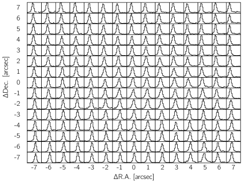
Figure 19: Reproduction of Figure 20 of Amram et al. (2003), but for our WiFeS observations: the H$\alpha$ line profile for all the spaxels within a box of 15$\times$15 arcsec² centered on the galaxy’s core (i.e. spaxel [0;0] in our reference frame). Each panel contains 19 wavelengths bins ranging from 6719.56Å to 6727.48Å. Each panel is normalized to the emission line peak.

As we find no evidence for multiple kinematics components in our WiFeS observations of HCG 91c - and especially find no evidence for the complex line profiles reported by Amram et al. (2003) - we are lead to conclude that the gas in this galaxy can be well described by a single kinematic structure at all locations.

Appendix B Error propagation in pyqz v0.6.0

In the original version published by Dopita et al. (2013b), the pyqz v0.4.0 module was not set up to account for errors in the flux measurements of emission lines. Instead, errors on the estimation of $\log$(q) and 12+$\log$(O/H) were estimated from the standard deviation between the different estimates stemming from the different line ratio diagnostic grids chosen by the user. Indeed, for flux measurements at the $\sim$5% level, the mismatch between the estimates from different diagnostics typically dominates the uncertainty of the joint final estimate. For larger observational errors on the emission line fluxes, pyqz v0.4.0 therefore under-estimates the true error associated with the final values of 12+$\log$(O/H) and $\log$(q). Here, we have upgraded pyqz to address this shortcoming. The updated version of pyqz will be publicly released and described in details in the near future along with new mappings iv models. Here, we briefly describe for completeness how errors on the final 12+$\log$(O/H) and $\log$(q) estimates in our analysis of HCG 91c are computed.

The underlying idea is to propagate the full probability density function associated with each line flux measurement to the 12+$\log$(O/H) vs $\log$(q) plane. To that end, for each set of line fluxes (and errors) provided by the user (i.e. for each individual spaxel, in the case of our analysis), pyqz v0.6.0 generates $n$ random set of line fluxes from the errors provided by the user, assuming a normal and uncorrelated error distribution for each line. pyqz subsequently derives an estimate of 12+$\log$(O/H) and $\log$(q) for all $n$ set of random line fluxes, and for every line ratio diagnostic grid selected by the user, resulting in $n\times m$ estimates of 12+$\log$(O/H) and $\log$(q) (where $m$ is the number of line ratio grids selected by the user). Effectively, these $n\times m$ estimates represent the discretized two-dimensional joint probability distribution function of the oxygen abundance and ionization parameter. The full joint probability density function can the be reconstructed by performing a two-dimensional kernel density estimation. This frequentist approach to error estimation differs from the Bayes formalism adopted by Blanc et al. (2014) in the izi code written in idl with a similar purpose to pyqz.

It is often practical to derive from the joint probability density function a best-estimate and associated uncertainty. To derive the best estimate for 12+$\log$(O/H) and $\log$(q), pyqz normalizes the reconstructed joint probability function to its peak level, and computes the 61%-level contour (corresponding the 1-sigma level for a normal distribution). The mean location of this contour is then chosen as the best estimate of the 12+$\log$(O/H) and $\log$(q), while the full extent of the contour is indicative of the uncertainty associated with these estimates.

The process is illustrated for two representative high and low S/N spaxels in our WiFeS observations of HCG 91c in Figures 20 and 21, respectively. For reasons detailed in Section 4.3, these examples rely on only two line ratio diagnostic grids: $\log$ $[$N II$]$/[S II] vs $\log$ [O III]/H$\beta$ and $\log$ $[$N II$]$/[S II] vs $\log$ [O III]/[S II]. The location of the individual estimates stemming from either diagnostic grids in the 12+$\log$(O/H) vs $\log$(q) are marked with white squares. The mean of these positions, corresponding to the pyqz v0.4.0 estimate of 12+$\log$(O/H) and $\log$(q), is marked with a white star. For both spaxels, 1000 random set of line fluxes were generated by pyqz, resulting in 2000 estimates of 12+$\log$(O/H) and $\log$(q) (1000 for either line ratio grid), shown as individual red dots.

The 61%-of-peak-level contour of the underlying reconstructed joint probability density function is shown with an orange line. With 1000 random sets of line fluxes, we find that the location of the peak of the joint probability density function (marked with an orange diamond symbol) varies within the 1-sigma contours when pyqz is run multiple times. However, the location of the 1-sigma contour at 61% of the peak level remains consistent when pyqz is run multiple times. This fact motivates our choice to base the final estimates of 12+$\log$(O/H) and $\log$(q) on the mean location of the 1-sigma contour level, rather than the exact peak location.

Different python tools exists to perform a two-dimensional kernel density estimation. pyqz can be set by the user to use two of these - either the gaussian_kde routine in the scipy.stats package , or the kdemultivariate routine in the statsmodel package . The former routine is 10-100 times faster but is not well suited for bi- or multi-modal distributions. In the case of pyqz, the gaussian_kde routine tends to over-smooth the joint probability function when two diagnostics are not directly consistent with one another (for example in the case of a flux measurement error). The option to use the gaussian_kde routine is included in pyqz v0.6.0 as a rapid alternative to test the code and obtain preliminary results. In practice, it is preferable to use the kdemultivariate routine instead which provides more accurate results, as the bandwidth of the gaussian kernel can be set individually for the 12+$\log$(O/H) and $\log$(q) directions. All estimates of oxygen abundances and ionization parameters presented in this article were derived using the kdemultivariate method.

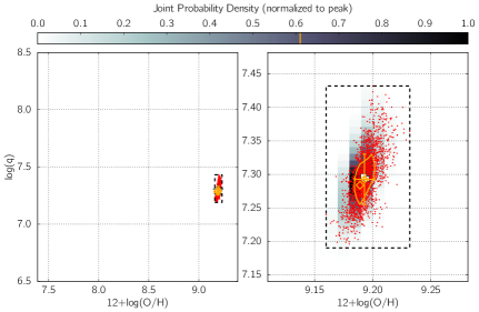
Figure 20: Full (left) and magnified (right) oxygen abundance and ionization parameter plane accessible to pyqz v0.6.0. The data corresponds to the spaxel [0;0] in our observations of HCG 91c. The white squares mark the two estimates associated with the diagnostic grids $\log$ $[$N II$]$/[S II] vs $\log$ [O III]/H$\beta$ and $\log$ $[$N II$]$/[S II] vs $\log$ [O III]/[S II]. The red dots mark the location of 2$\times$1000 randomly-reconstructed line fluxes from the original line fluxes and associated errors. The reconstructed 2-D joint probability density distribution (with a fixed resolution of 0.01 in 12+$\log$(O/H) and 0.01 in $\log$(q)) is also shown, with the orange contour tracing the 1-sigma level from the peak. The peak location is marked with an orange diamond, while the mean location of the 1-sigma contour and its extent in marked with the orange circle and associated error bars. The dashed box marks the full extent of the random set of individual estimates (the red dots).

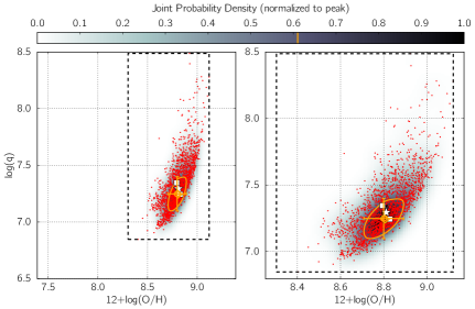
Figure 21: Same as Figure 20, but for the spaxel [9;14]. The lower S/N in the data results in a larger spread of the random set of estimates.

References

- Allen et al. (2008) Allen M. G., Groves B. A., Dopita M. A., Sutherland R. S., Kewley L. J., 2008, ApJS, 178, 20
- Amram et al. (2003) Amram P., Plana H., Mendes de Oliveira C., Balkowski C., Boulesteix J., 2003, A&A, 402, 865
- Appleton et al. (2006) Appleton P. N., et al., 2006, ApJL, 639, L51
- Astropy Collaboration et al. (2013) Astropy Collaboration et al., 2013, A&A, 558, A33
- Bacon et al. (2001) Bacon R., et al., 2001, MNRAS, 326, 23
- Bacon et al. (2010) Bacon R., et al., 2010, in Society of Photo-Optical Instrumentation Engineers (SPIE) Conference Series, 7735, 773508. , doi:10.1117/12.856027
- Barnes & Fluke (2008) Barnes D. G., Fluke C. J., 2008, New A, 13, 599
- Barnes & Webster (2001) Barnes D. G., Webster R. L., 2001, MNRAS, 324, 859
- Belokurov et al. (2006) Belokurov V., et al., 2006, ApJL, 642, L137
- Binette et al. (1982) Binette L., Dopita M. A., Dodorico S., Benvenuti P., 1982, A&A, 115, 315
- Binette et al. (1985) Binette L., Dopita M. A., Tuohy I. R., 1985, ApJ, 297, 476
- Bitsakis et al. (2014) Bitsakis T., Charmandaris V., Appleton P. N., Díaz-Santos T., Le Floc’h E., da Cunha E., Alatalo K., Cluver M., 2014, A&A, 565, A25
- Blanc et al. (2013) Blanc G. A., et al., 2013, AJ, 145, 138
- Blanc et al. (2014) Blanc G. A., Kewley L., Vogt F. P. A., Dopita M. A., 2014, ArXiv e-prints,
- Bonnarel et al. (2000) Bonnarel F., et al., 2000, A&AS, 143, 33
- Borthakur et al. (2010) Borthakur S., Yun M. S., Verdes-Montenegro L., 2010, ApJ, 710, 385
- Bundy et al. (2014) Bundy K., et al., 2014, arXiv:1412.1482,
- Calzetti et al. (2000) Calzetti D., Armus L., Bohlin R. C., Kinney A. L., Koornneef J., Storchi-Bergmann T., 2000, ApJ, 533, 682
- Calzetti et al. (2007) Calzetti D., et al., 2007, ApJ, 666, 870
- Cappellari & Emsellem (2004) Cappellari M., Emsellem E., 2004, PASP, 116, 138
- Cappellari et al. (2007) Cappellari M., et al., 2007, MNRAS, 379, 418
- Cappellari et al. (2011) Cappellari M., et al., 2011, MNRAS, 413, 813
- Childress et al. (2014a) Childress M., Vogt F., Nielsen J., Sharp R., 2014a, PyWiFeS: Wide Field Spectrograph data reduction pipeline, ascl:1402.034
- Childress et al. (2014b) Childress M. J., Vogt F. P. A., Nielsen J., Sharp R. G., 2014b, Ap&SS, 349, 617
- Cluver et al. (2010) Cluver M. E., et al., 2010, ApJ, 710, 248
- Cluver et al. (2013) Cluver M. E., et al., 2013, ApJ, 765, 93
- Cortese et al. (2006) Cortese L., Gavazzi G., Boselli A., Franzetti P., Kennicutt R. C., O’Neil K., Sakai S., 2006, A&A, 453, 847
- Coziol & Plauchu-Frayn (2007) Coziol R., Plauchu-Frayn I., 2007, AJ, 133, 2630
- Croom et al. (2012) Croom S. M., et al., 2012, MNRAS, 421, 872
- Cybulski et al. (2014) Cybulski R., Yun M. S., Fazio G. G., Gutermuth R. A., 2014, MNRAS, 439, 3564
- Desjardins et al. (2013) Desjardins T. D., et al., 2013, ApJ, 763, 121
- Desjardins et al. (2014) Desjardins T. D., et al., 2014, ApJ, 790, 132
- Dopita et al. (1982) Dopita M. A., Binette L., Schwartz R. D., 1982, ApJ, 261, 183
- Dopita et al. (2006) Dopita M. A., et al., 2006, ApJS, 167, 177
- Dopita et al. (2007) Dopita M., Hart J., McGregor P., Oates P., Bloxham G., Jones D., 2007, Ap&SS, 310, 255
- Dopita et al. (2010) Dopita M., et al., 2010, Ap&SS, 327, 245
- Dopita et al. (2013a) Dopita M. A., Rich J., Vogt F. P. A., Kewley L. J., Ho I.-T., Basurah H. M., Ali A., Amer M. A., 2013a, Ap&SS,
- Dopita et al. (2013b) Dopita M. A., Sutherland R. S., Nicholls D. C., Kewley L. J., Vogt F. P. A., 2013b, ApJS, 208, 10
- Dopita et al. (2014a) Dopita M. A., et al., 2014a, ArXiv e-prints,
- Dopita et al. (2014b) Dopita M. A., et al., 2014b, A&A, 566, A41
- Driver et al. (2009) Driver S. P., et al., 2009, Astronomy and Geophysics, 50, 050000
- Drory et al. (2014) Drory N., et al., 2014, arXiv e-prints:1412.1535,
- Emsellem et al. (2004) Emsellem E., et al., 2004, MNRAS, 352, 721
- Fischera & Dopita (2005) Fischera J., Dopita M., 2005, ApJ, 619, 340
- Fitzpatrick (1999) Fitzpatrick E. L., 1999, PASP, 111, 63
- Gallagher et al. (2008) Gallagher S. C., Johnson K. E., Hornschemeier A. E., Charlton J. C., Hibbard J. E., 2008, ApJ, 673, 730
- Gentile et al. (2013) Gentile G., et al., 2013, A&A, 554, A125
- Gillmon & Shull (2006) Gillmon K., Shull J. M., 2006, ApJ, 636, 908
- González Delgado et al. (2005) González Delgado R. M., Cerviño M., Martins L. P., Leitherer C., Hauschildt P. H., 2005, MNRAS, 357, 945
- Groves et al. (2004) Groves B. A., Dopita M. A., Sutherland R. S., 2004, ApJS, 153, 9
- Heald et al. (2011) Heald G., et al., 2011, A&A, 526, A118
- Hickson (1982a) Hickson P., 1982a, ApJ, 255, 382
- Hickson (1982b) Hickson P., 1982b, ApJ, 259, 930
- Hickson et al. (1992) Hickson P., Mendes de Oliveira C., Huchra J. P., Palumbo G. G., 1992, ApJ, 399, 353
- Ho et al. (2014) Ho I.-T., et al., 2014, MNRAS, 444, 3894
- Hodapp et al. (2004) Hodapp K. W., et al., 2004, Astronomische Nachrichten, 325, 636
- Hunter (2007) Hunter J. D., 2007, Computing In Science & Engineering, 9, 90
- Iovino (2002) Iovino A., 2002, AJ, 124, 2471
- Johnson et al. (2007) Johnson K. E., Hibbard J. E., Gallagher S. C., Charlton J. C., Hornschemeier A. E., Jarrett T. H., Reines A. E., 2007, AJ, 134, 1522
- Jones et al. (2004) Jones D. H., et al., 2004, MNRAS, 355, 747
- Jones et al. (2009) Jones D. H., et al., 2009, MNRAS, 399, 683
- Kaiser (2004) Kaiser N., 2004, in Oschmann Jr. J. M., ed., Society of Photo-Optical Instrumentation Engineers (SPIE) Conference Series Vol. 5489, Ground-based Telescopes. pp 11–22, doi:10.1117/12.552472
- Kaiser et al. (2002) Kaiser N., et al., 2002, in Tyson J. A., Wolff S., eds, Society of Photo-Optical Instrumentation Engineers (SPIE) Conference Series Vol. 4836, Survey and Other Telescope Technologies and Discoveries. pp 154–164, doi:10.1117/12.457365
- Kaiser et al. (2010) Kaiser N., et al., 2010, in Society of Photo-Optical Instrumentation Engineers (SPIE) Conference Series, 7733, 77330E. , doi:10.1117/12.859188
- Kalberla & Kerp (2009) Kalberla P. M. W., Kerp J., 2009, ARA&A, 47, 27
- Kamphuis et al. (2013) Kamphuis P., et al., 2013, MNRAS, 434, 2069
- Kauffmann et al. (2003) Kauffmann G., et al., 2003, MNRAS, 346, 1055
- Kennicutt (1998) Kennicutt Jr. R. C., 1998, ApJ, 498, 541
- Kennicutt & Evans (2012) Kennicutt R. C., Evans N. J., 2012, ARA&A, 50, 531
- Kent (2013) Kent B. R., 2013, PASP, 125, 731
- Kewley et al. (2001) Kewley L. J., Heisler C. A., Dopita M. A., Lumsden S., 2001, ApJS, 132, 37
- Kewley et al. (2006) Kewley L. J., Groves B., Kauffmann G., Heckman T., 2006, MNRAS, 372, 961
- Kewley et al. (2010) Kewley L. J., Rupke D., Zahid H. J., Geller M. J., Barton E. J., 2010, ApJL, 721, L48
- Komatsu et al. (2011) Komatsu E., et al., 2011, ApJS, 192, 18
- Krajnović et al. (2006) Krajnović D., Cappellari M., de Zeeuw P. T., Copin Y., 2006, MNRAS, 366, 787
- Krajnović et al. (2011) Krajnović D., et al., 2011, MNRAS, 414, 2923
- Kroupa (2001) Kroupa P., 2001, MNRAS, 322, 231
- Lara-López et al. (2013) Lara-López M. A., et al., 2013, MNRAS, 434, 451
- Lauberts & Valentijn (1989) Lauberts A., Valentijn E. A., 1989, The surface photometry catalogue of the ESO-Uppsala galaxies
- Leitherer et al. (1999) Leitherer C., et al., 1999, ApJS, 123, 3
- Magnier (2007) Magnier E., 2007, in Sterken C., ed., Astronomical Society of the Pacific Conference Series Vol. 364, The Future of Photometric, Spectrophotometric and Polarimetric Standardization. p. 153
- Magnier et al. (2013) Magnier E. A., et al., 2013, ApJS, 205, 20
- Marasco & Fraternali (2011) Marasco A., Fraternali F., 2011, A&A, 525, A134
- Markwardt (2009) Markwardt C. B., 2009, in Bohlender D. A., Durand D., Dowler P., eds, Astronomical Society of the Pacific Conference Series Vol. 411, Astronomical Data Analysis Software and Systems XVIII. p. 251, arXiv:0902.2850
- Mathewson et al. (2013) Mathewson D. S., Hart J., Wehner H. P., Hovey G. R., van Harmelen J., 2013, Journal of Astronomical History and Heritage, 16, 2
- Mendes de Oliveira et al. (2003) Mendes de Oliveira C., Amram P., Plana H., Balkowski C., 2003, AJ, 126, 2635
- Moore et al. (1998) Moore B., Lake G., Katz N., 1998, ApJ, 495, 139
- Murphy et al. (2011) Murphy E. J., et al., 2011, ApJ, 737, 67
- Nicholls et al. (2012) Nicholls D. C., Dopita M. A., Sutherland R. S., 2012, ApJ, 752, 148
- Nicholls et al. (2013) Nicholls D. C., Dopita M. A., Sutherland R. S., Kewley L. J., Palay E., 2013, ApJS, 207, 21
- Oosterloo et al. (2007) Oosterloo T., Fraternali F., Sancisi R., 2007, AJ, 134, 1019
- Osterbrock (1989) Osterbrock D. E., 1989, Astrophysics of gaseous nebulae and active galactic nuclei
- Plauchu-Frayn et al. (2012) Plauchu-Frayn I., Del Olmo A., Coziol R., Torres-Papaqui J. P., 2012, A&A, 546, A48
- Ponman et al. (1996) Ponman T. J., Bourner P. D. J., Ebeling H., Böhringer H., 1996, MNRAS, 283, 690
- Putman et al. (2012) Putman M. E., Peek J. E. G., Joung M. R., 2012, ARA&A, 50, 491
- Ramachandran & Varoquaux (2011) Ramachandran P., Varoquaux G., 2011, Computing in Science & Engineering, 13, 40
- Rasmussen et al. (2008) Rasmussen J., Ponman T. J., Verdes-Montenegro L., Yun M. S., Borthakur S., 2008, MNRAS, 388, 1245
- Rasmussen et al. (2012) Rasmussen J., Mulchaey J. S., Bai L., Ponman T. J., Raychaudhury S., Dariush A., 2012, ApJ, 757, 122
- Renaud et al. (2008) Renaud F., Boily C. M., Fleck J.-J., Naab T., Theis C., 2008, MNRAS, 391, L98
- Renaud et al. (2009) Renaud F., Boily C. M., Naab T., Theis C., 2009, ApJ, 706, 67
- Renaud et al. (2014) Renaud F., Bournaud F., Kraljic K., Duc P.-A., 2014, MNRAS, 442, L33
- Rich et al. (2010) Rich J. A., Dopita M. A., Kewley L. J., Rupke D. S. N., 2010, ApJ, 721, 505
- Richardson et al. (2011) Richardson J. C., et al., 2011, ApJ, 732, 76
- Richter et al. (2003) Richter P., Wakker B. P., Savage B. D., Sembach K. R., 2003, ApJ, 586, 230
- Röhser et al. (2014) Röhser T., Kerp J., Winkel B., Boulanger F., Lagache G., 2014, A&A, 564, A71
- Rosales-Ortega et al. (2010) Rosales-Ortega F. F., Kennicutt R. C., Sánchez S. F., Díaz A. I., Pasquali A., Johnson B. D., Hao C. N., 2010, MNRAS, 405, 735
- Rubin et al. (1991) Rubin V. C., Hunter D. A., Ford Jr. W. K., 1991, ApJS, 76, 153
- Rupke et al. (2010) Rupke D. S. N., Kewley L. J., Chien L.-H., 2010, ApJ, 723, 1255
- Sánchez et al. (2012) Sánchez S. F., et al., 2012, A&A, 538, A8
- Saul et al. (2012) Saul D. R., et al., 2012, ApJ, 758, 44
- Schlafly & Finkbeiner (2011) Schlafly E. F., Finkbeiner D. P., 2011, ApJ, 737, 103
- Schlegel et al. (1998) Schlegel D. J., Finkbeiner D. P., Davis M., 1998, ApJ, 500, 525
- Seabold & Perktold (2010) Seabold J. S., Perktold J., 2010, in Proceedings of the 9th Python in Science Conference. pp 57–61
- Skrutskie et al. (2006) Skrutskie M. F., et al., 2006, AJ, 131, 1163
- Sutherland & Dopita (1993) Sutherland R. S., Dopita M. A., 1993, ApJS, 88, 253
- Tonry et al. (2012) Tonry J. L., et al., 2012, ApJ, 750, 99
- Torres-Flores et al. (2010) Torres-Flores S., Mendes de Oliveira C., Amram P., Plana H., Epinat B., Carignan C., Balkowski C., 2010, A&A, 521, A59
- Torres-Flores et al. (2013) Torres-Flores S., Mendes de Oliveira C., Plana H., Amram P., Epinat B., 2013, MNRAS, 432, 3085
- Tzanavaris et al. (2010) Tzanavaris P., et al., 2010, ApJ, 716, 556
- Verdes-Montenegro et al. (2001) Verdes-Montenegro L., Yun M. S., Williams B. A., Huchtmeier W. K., Del Olmo A., Perea J., 2001, A&A, 377, 812
- Vijayaraghavan & Ricker (2013) Vijayaraghavan R., Ricker P. M., 2013, MNRAS, 435, 2713
- Vogt et al. (2013) Vogt F. P. A., Dopita M. A., Kewley L. J., 2013, ApJ, 768, 151
- Wakker (2001) Wakker B. P., 2001, ApJS, 136, 463
- Wakker (2006) Wakker B. P., 2006, ApJS, 163, 282
- Wakker & van Woerden (1997) Wakker B. P., van Woerden H., 1997, ARA&A, 35, 217
- Walker et al. (2010) Walker L. M., Johnson K. E., Gallagher S. C., Hibbard J. E., Hornschemeier A. E., Tzanavaris P., Charlton J. C., Jarrett T. H., 2010, AJ, 140, 1254
- Walker et al. (2012) Walker L. M., Johnson K. E., Gallagher S. C., Charlton J. C., Hornschemeier A. E., Hibbard J. E., 2012, AJ, 143, 69
- Weiß et al. (1999) Weiß A., Heithausen A., Herbstmeier U., Mebold U., 1999, A&A, 344, 955
- Westmoquette et al. (2007) Westmoquette M. S., Exter K. M., Smith L. J., Gallagher J. S., 2007, MNRAS, 381, 894
- Wijesinghe et al. (2011) Wijesinghe D. B., et al., 2011, MNRAS, 410, 2291
- Zschaechner et al. (2011) Zschaechner L. K., Rand R. J., Heald G. H., Gentile G., Kamphuis P., 2011, ApJ, 740, 35
- Zschaechner et al. (2012) Zschaechner L. K., Rand R. J., Heald G. H., Gentile G., Józsa G., 2012, ApJ, 760, 37
- de Vaucouleurs et al. (1991) de Vaucouleurs G., de Vaucouleurs A., Corwin Jr. H. G., Buta R. J., Paturel G., Fouqué P., 1991, Third Reference Catalogue of Bright Galaxies. Volume I: Explanations and references. Volume II: Data for galaxies between 0h and 12h. Volume III: Data for galaxies between 12h and 24h.
- de Zeeuw et al. (2002) de Zeeuw P. T., et al., 2002, MNRAS, 329, 513
- de la Rosa et al. (2007) de la Rosa I. G., de Carvalho R. R., Vazdekis A., Barbuy B., 2007, AJ, 133, 330