Position-dependent correlation function from the SDSS-III Baryon Oscillation Spectroscopic Survey Data Release 10 CMASS Sample

Abstract

We report on the first measurement of the three-point function with the position-dependent correlation function from the SDSS-III Baryon Oscillation Spectroscopic Survey (BOSS) Data Release 10 CMASS sample. This new observable measures the correlation between two-point functions of galaxy pairs within different subvolumes, $\hat{\xi}(\mathbf{r},\mathbf{r}_{L})$, where $\mathbf{r}_{L}$ is the location of a subvolume, and the corresponding mean overdensities, $\bar{\delta}(\mathbf{r}_{L})$. This correlation, which we call the “integrated three-point function”, $i\zeta(r)\equiv\langle\hat{\xi}(\mathbf{r},\mathbf{r}_{L})\bar{\delta}(\mathbf{r}_{L})\rangle$, measures a three-point function of two short- and one long-wavelength modes, and is generated by nonlinear gravitational evolution and possibly also by the physics of inflation. The $i\zeta(r)$ measured from the BOSS data lies within the scatter of those from the mock galaxy catalogs in redshift space, yielding a ten-percent-level determination of the amplitude of $i\zeta(r)$. The tree-level perturbation theory in redshift space predicts how this amplitude depends on the linear and quadratic nonlinear galaxy bias parameters ($b_{1}$ and $b_{2}$), as well as on the amplitude and linear growth rate of matter fluctuations ($\sigma_{8}$ and $f$). Combining $i\zeta(r)$ with the constraints on $b_{1}\sigma_{8}$ and $f\sigma_{8}$ from the global two-point correlation function and that on $\sigma_{8}$ from the weak lensing signal of BOSS galaxies, we measure $b_{2}=0.41\pm 0.41$ (68% C.L.) assuming standard perturbation theory at the tree level and the local bias model.

1 Introduction

Mode coupling plays a fundamental role in cosmology. A long-wavelength scalar density fluctuation modifies the formation of small-scale structure via gravitational evolution (see [1] for a review), and possibly also through the physics of inflation. This effect of long-wavelength modes manifests itself through a dependence of observables, e.g., the $n$-point statistics and the halo mass function, on the local long-wavelength overdensity, or equivalently, the position in space (see [2, 3, 4] for the $n$-point statistics and [5, 6] for the mass function). Measurements of spatially-varying, “position-dependent” observables capture the effects of mode coupling, and can be used to test our understanding of gravity and the physics of inflation. A similar idea of measuring the shift of the peak position of the baryonic acoustic oscillation in different environments has been studied in ref. [7].

In this paper, we focus on the position-dependent two-point function. Consider a galaxy redshift survey. Instead of measuring the two-point function of galaxy pairs within the entire survey volume, we divide the survey volume into many subvolumes, within which we measure the two-point function of galaxy pairs. These two-point functions vary spatially from subvolume to subvolume, and the variation is correlated with the mean overdensities of the subvolumes with respect to the entire survey volume. As we show later in detail, this correlation measures an integral of the three-point function, which represents the response of the small-scale clustering of galaxies (as measured by the position-dependent two-point functions) to the long-wavelength density perturbation (as measured by the mean overdensities of the subvolumes) [2].

Not only is the position-dependent correlation function conceptually straightforward to interpret, but the computational requirement for measuring three-point statistics is also largely alleviated. The usual three-point correlation function measurements rely on finding particle triplets with the naive algorithm scaling as $N_{\rm par}^{3}$ where $N_{\rm par}$ is the number of particles. Current galaxy redshift surveys contain roughly a million galaxies, and we need 50 times as many random samples as the galaxies for characterizing the survey window function accurately (see, e.g., [8]). Counting triplets thus becomes computationally challenging. Similarly, the measurement of the three-point function in Fourier space, i.e., the bispectrum, requires counting of all possible triangle configurations formed by different Fourier modes, which is also computationally demanding. This explains why only few measurements of the three-point function of the large-scale structure have been reported in the literature [9, 10, 11, 12, 13, 14, 15, 16, 17].

The computational requirement is alleviated for the position-dependent correlation function technique because we explore a subset of triplets corresponding to the “squeezed configurations” of the three-point function; namely, two short-wavelength modes correlated with one long-wavelength mode. We only need to count particle pairs for measuring the two-point function in subvolumes, which scales as $N_{\rm par}^{2}$. The scaling is further improved because the number of particles in each subvolume decreases by the number of the subvolumes $N_{s}$; hence, it scales as $N_{s}(N_{\rm par}/N_{s})^{2}=N_{\rm par}^{2}/N_{s}$. The position-dependent correlation function technique is thus particularly efficient for extracting the information of the squeezed-limit bispectrum, which we shall demonstrate in appendix D, while it is relatively insensitive to the bispectrum in other configurations.

In this paper, we report on the first measurement of the three-point function with the position-dependent correlation function from the SDSS-III Baryon Oscillation Spectroscopic Survey Data Release 10 (hereafter BOSS DR10) CMASS sample [18, 19]. We compare this measurement with those from the PTHalos mock catalogs [20, 21, 22]. While the mocks were designed to reproduce the global two-point function of the BOSS DR10 CMASS sample, it is not guaranteed that they can reproduce the three-point function as measured by the position-dependent correlation function. We shall show that the position-dependent correlation functions from the real data and the mocks are consistent with each other. Finally, we use tree-level perturbation theory to predict the position-dependent correlation function as a function of the galaxy bias parameters and the cosmological parameters, and determine the quadratic nonlinear bias parameter of the BOSS DR10 CMASS sample by combining the constraints from the position-dependent correlation function, the global two-point function, and the weak lensing signal.

The rest of the paper is organized as follows. In section 2, we define the position-dependent correlation function and the integrated three-point function, and describe the tree-level perturbation theory prediction for the integrated three-point function in redshift space. In section 3 and 4, we apply the position-dependent correlation function technique to the mocks and the BOSS DR10 CMASS sample, respectively. The cosmological interpretation of the measurements is given in section 5. We conclude in section 6. In appendix A, we test our estimator using Gaussian realizations. In appendix B, we study the effects of using extended models of the bispectrum with the effective $F_{2}$ and $G_{2}$ kernels and a tidal bias. In appendix C, we compare the mocks and BOSS DR10 CMASS samples in different redshift bins. In appendix D, we use the Fisher matrix calculation to demonstrate the information content of the position-dependent correlation function. Throughout the paper we adopt the cosmology of the mocks as our fiducial cosmology, i.e., a flat $\Lambda$CDM cosmology with $\Omega_{m}=0.274$, $\Omega_{b}h^{2}=0.0224$, $h=0.7$, $\sigma_{8}=0.8$, and $n_{s}=0.95$.

2 Position-dependent correlation function and the integrated three-point function in redshift space

2.1 Position-dependent correlation function

Consider a density fluctuation field, $\delta({\bf r})$, in a survey (or simulation) volume $V_{r}$. The mean overdensity of this volume vanishes by construction, i.e., $\bar{\delta}=\frac{1}{V_{r}}\int_{V_{r}}d^{3}r~{}\delta({\bf r})=0$. The global two-point function is defined as

$$\xi(r)=\langle\delta(\mathbf{x})\delta(\mathbf{x}+\mathbf{r})\rangle~{},$$ (2.1)

where we assume that $\delta({\bf r})$ is statistically homogeneous and isotropic, so $\xi(r)$ depends only on the separation $r$. As the ensemble average cannot be measured directly, we estimate the global two-point function as

$$\hat{\xi}(r)=\frac{1}{V_{r}}\int\frac{d^{2}\hat{\mathbf{r}}}{4\pi}\int_{\mathbf{x},\mathbf{x}+\mathbf{r}\in V_{r}}d^{3}x~{}\delta(\mathbf{r}+\mathbf{x})\delta(\mathbf{x})\,.$$ (2.2)

The ensemble average of eq. (2.2) is not equal to $\xi(r)$. Specifically,

$$\langle\hat{\xi}(r)\rangle=\> \frac{1}{V_{r}}\int\frac{d^{2}\hat{r}}{4\pi}\int_{\mathbf{x},\mathbf{x}+\mathbf{r}\in V_{r}}d^{3}x~{}\langle\delta(\mathbf{r}+\mathbf{x})\delta(\mathbf{x})\rangle=\xi(r)\frac{1}{V_{r}}\int\frac{d^{2}\hat{r}}{4\pi}\int_{\mathbf{x},\mathbf{x}+\mathbf{r}\in V_{r}}d^{3}x~{}.$$ (2.3)

The second integral in eq. (2.3) is $V_{r}$ only if $\mathbf{r}=0$, and the fact that it departs from $V_{r}$ is due to the finite boundary of $V_{r}$. We shall quantify this boundary effect later in eq. (2.8).

We now identify a subvolume $V_{L}$ centered at $\mathbf{r}_{L}$, and compute the mean overdensity and the correlation function within $V_{L}$. The mean overdensity is

$$\bar{\delta}(\mathbf{r}_{L})=\frac{1}{V_{L}}\int_{V_{L}}d^{3}r~{}\delta({\bf r})=\frac{1}{V_{L}}\int d^{3}r~{}\delta({\bf r})W(\mathbf{r}-\mathbf{r}_{L})~{},$$ (2.4)

where $W(\mathbf{r})$ is the window function. Throughout this paper, we use a cubic window function given by

$$W(\mathbf{r})=W_{L}(\mathbf{r})=\prod_{i=1}^{3}\>\theta(r_{i}),\quad\theta(r_{i})=\left\{\begin{array}[]{cc}1,&|r_{i}|\leq L/2,\\ 0,&\mbox{otherwise}~{},\end{array}\right.$$ (2.5)

where $L$ is the side length of $V_{L}$. The results are not sensitive to the exact choice of the window function, provided that the separation between galaxy pairs is much smaller than $L$. While $\bar{\delta}=0$, $\bar{\delta}(\mathbf{r}_{L})$ is non-zero in general. In other words, if $\bar{\delta}(\mathbf{r}_{L})$ is positive (negative), then this subvolume is overdense (underdense) with respect to the mean density in $V_{r}$.

Using the same window function, we define the position-dependent correlation function in the subvolume $V_{L}$ centered at $\mathbf{r}_{L}$ as

$$\hat{\xi}(\mathbf{r},\mathbf{r}_{L})=\> \frac{1}{V_{L}}\int\displaylimits_{\mathbf{x},\mathbf{r}+\mathbf{x}\in V_{L}}d^{3}x~{}\delta(\mathbf{r}+\mathbf{x})\delta(\mathbf{x})$$

$$=\> \frac{1}{V_{L}}\int d^{3}x~{}\delta(\mathbf{r}+\mathbf{x})\delta(\mathbf{x})W_{L}(\mathbf{r}+\mathbf{x}-\mathbf{r}_{L})W_{L}(\mathbf{x}-\mathbf{r}_{L})~{}.$$ (2.6)

This is essentially an estimator for a local two-point function. In this paper we shall consider only the angle-averaged position-dependent correlation function (i.e., the monopole) defined by

$$\hat{\xi}(r,\mathbf{r}_{L})=\int\frac{d^{2}\hat{r}}{4\pi}~{}\hat{\xi}(\mathbf{r},\mathbf{r}_{L})=\frac{1}{V_{L}}\int\frac{d^{2}\hat{r}}{4\pi}\int d^{3}x~{}\delta(\mathbf{r}+\mathbf{x})\delta(\mathbf{x})W_{L}(\mathbf{r}+\mathbf{x}-\mathbf{r}_{L})W_{L}(\mathbf{x}-\mathbf{r}_{L})~{}.$$ (2.7)

Similarly to that of the global two-point function, the ensemble average of eq. (2.7) is not equal to $\xi(r)$. Specifically,

$$\langle\hat{\xi}(r,\mathbf{r}_{L})\rangle=\> \frac{1}{V_{L}}\int\frac{d^{2}\hat{r}}{4\pi}\int d^{3}x~{}\langle\delta(\mathbf{r}+\mathbf{x})\delta(\mathbf{x})\rangle W_{L}(\mathbf{r}+\mathbf{x}-\mathbf{r}_{L})W_{L}(\mathbf{x}-\mathbf{r}_{L})$$

$$=\> \xi(r)\frac{1}{V_{L}}\int\frac{d^{2}\hat{r}}{4\pi}\int d^{3}x^{\prime}~{}W_{L}(\mathbf{r}+\mathbf{x}^{\prime})W_{L}(\mathbf{x}^{\prime})\equiv\xi(r)f_{\rm bndry}(r)~{},$$ (2.8)

where $f_{\rm bndry}(r)$ is the boundary effect due to the finite size of the subvolume. While $f_{\rm bndry}(r)=1$ for $r=0$, the boundary effect becomes larger for larger separations. The boundary effect can be computed by the five-dimensional integral in eq. (2.8). Alternatively, it can be evaluated by the ratio of the number of the random particle pairs of a given separation in a finite volume to the expected random particle pairs in the shell with the same separation in an infinite volume. We have evaluated $f_{\rm bndry}(r)$ in both ways, and the results are in an excellent agreement.

As the usual two-point function estimators based on pair counting (such as Landy-Szalay estimator which will be discussed in section 3.2) or grid counting (which will be discussed in appendix A) do not contain the boundary effect, when we compare the measurements to the model which is calculated based on eq. (2.7), we shall divide the model by $f_{\rm bndry}(r)$ to correct for the boundary effect.

2.2 Integrated three-point function

The correlation between $\hat{\xi}(r,\mathbf{r}_{L})$ and $\bar{\delta}(\mathbf{r}_{L})$ is given by

$$\langle\hat{\xi}(r,\mathbf{r}_{L})\bar{\delta}(\mathbf{r}_{L})\rangle=\> \frac{1}{V_{L}^{2}}\int\frac{d^{2}\hat{r}}{4\pi}\int d^{3}x_{1}\int d^{3}x_{2}~{}\langle\delta(\mathbf{r}+\mathbf{x}_{1})\delta(\mathbf{x}_{1})\delta(\mathbf{x}_{2})\rangle$$

$$~{}~{}~{}~{}~{}~{}~{}~{}~{}~{}~{}~{}~{}~{}~{}~{}~{}~{}~{}~{}~{}~{}~{}~{}~{}~{}~{}~{}~{}~{}~{}~{}~{}~{}\times W_{L}(\mathbf{r}+\mathbf{x}_{1}-\mathbf{r}_{L})W_{L}(\mathbf{x}_{1}-\mathbf{r}_{L})W_{L}(\mathbf{x}_{2}-\mathbf{r}_{L})$$

$$=\> \frac{1}{V_{L}^{2}}\int\frac{d^{2}\hat{r}}{4\pi}\int d^{3}x_{1}\int d^{3}x_{2}~{}\zeta(\mathbf{r}+\mathbf{x}_{1}+\mathbf{r}_{L},\mathbf{x}_{1}+\mathbf{r}_{L},\mathbf{x}_{2}+\mathbf{r}_{L})$$

$$~{}~{}~{}~{}~{}~{}~{}~{}~{}~{}~{}~{}~{}~{}~{}~{}~{}~{}~{}~{}~{}~{}~{}~{}~{}~{}~{}~{}~{}~{}~{}~{}~{}~{}\times W_{L}(\mathbf{r}+\mathbf{x}_{1})W_{L}(\mathbf{x}_{1})W_{L}(\mathbf{x}_{2})~{},$$ (2.9)

where $\zeta(\mathbf{r}_{1},\mathbf{r}_{2},\mathbf{r}_{3})\equiv\langle\delta(\mathbf{r}_{1})\delta(\mathbf{r}_{2})\delta(\mathbf{r}_{3})\rangle$ is the three-point correlation function. Because of the assumption of homogeneity and isotropy, the three-point function depends only on the separations $|\mathbf{r}_{i}-\mathbf{r}_{j}|$ for $i\neq j$, and so $\langle\hat{\xi}(r,\mathbf{r}_{L})\bar{\delta}(\mathbf{r}_{L})\rangle$ is independent of $\mathbf{r}_{L}$. Furthermore, as the right-hand-side of eq. (2.9) is an integral of the three-point function, we will refer to this quantity as the “integrated three-point function,” $i\zeta(r)\equiv\langle\hat{\xi}(r,\mathbf{r}_{L})\bar{\delta}(\mathbf{r}_{L})\rangle$.

$i\zeta(r)$ can be computed if $\zeta(\mathbf{r}_{1},\mathbf{r}_{2},\mathbf{r}_{3})$ is known. For example, standard perturbation theory (SPT) with the local bias model at the tree level in real space gives

$$i\zeta(r)=b_{1}^{3}i\zeta_{\rm SPT}(r)+b_{1}^{2}b_{2}i\zeta_{b_{2}}(r)\,,$$ (2.10)

where $i\zeta_{\rm SPT}$ and $i\zeta_{b_{2}}$ are given below. Here, $b_{1}$ and $b_{2}$ are the linear and quadratic (nonlinear) bias parameters, respectively. Because of the high dimensionality of the integral, we use the Monte Carlo integration routine in the GNU Scientific Library to numerically evaluate $i\zeta(r)$. The first term, $i\zeta_{\rm SPT}$, is given by [23, 24]

$$\zeta_{\rm SPT}(\mathbf{r}_{1},\mathbf{r}_{2},\mathbf{r}_{3})=\> \frac{10}{7}\xi_{l}(r_{12})\xi_{l}(r_{23})+\mu_{12,23}[\xi_{l}^{\prime}(r_{12})\phi_{l}^{\prime}(r_{23})+\xi_{l}^{\prime}(r_{23})\phi_{l}^{\prime}(r_{12})]$$

$$+\frac{4}{7}\Bigg{\{}-3\frac{\phi_{l}^{\prime}(r_{12})\phi_{l}^{\prime}(r_{23})}{r_{12}r_{13}}-\frac{\xi_{l}(r_{12})\phi_{l}^{\prime}(r_{23})}{r_{23}}-\frac{\xi_{l}(r_{23})\phi_{l}^{\prime}(r_{12})}{r_{12}}$$

$$~{}~{}~{}~{}~{}~{}~{}~{}+\mu_{12,23}^{2}\left[\xi_{l}(r_{12})+\frac{3\phi_{l}^{\prime}(r_{12})}{r_{12}}\right]\left[\xi_{l}(r_{23})+\frac{3\phi_{l}^{\prime}(r_{23})}{r_{23}}\right]\Bigg{\}}$$

$$+2~{}{\rm cyclic}~{},$$ (2.11)

where $r_{12}=|\mathbf{r}_{1}-\mathbf{r}_{2}|$, $\mu_{12,23}$ is the cosine between $\mathbf{r}_{12}$ and $\mathbf{r}_{23}$, ^′ refers to the spatial derivative, and

$$\xi_{l}(r)\equiv\int\frac{dk}{2\pi^{2}}~{}k^{2}P_{l}(k){\rm sinc}(kr)\\ ,~{}~{}~{}~{}~{}~{}\phi_{l}(r)\equiv\int\frac{dk}{2\pi^{2}}~{}P_{l}(k){\rm sinc}(kr)\\ ,$$ (2.12)

with $P_{l}(k)$ being the linear matter power spectrum, and ${\rm sinc}(x)=\sin(x)/x$. The subscript $l$ denotes the quantities in the linear regime.

The second term, $i\zeta_{b_{2}}$, is the nonlinear local bias three-point function. Since halos (galaxies) are biased tracers of the underlying matter density field, the local bias prescription yields the density field of the biased tracers as $\delta_{h}(\mathbf{r})=b_{1}\delta_{m}(\mathbf{r})+\frac{b_{2}}{2}\delta_{m}^{2}(\mathbf{r})+...$, where $b_{1}$ and $b_{2}$ are the linear and nonlinear biases, respectively, and $\delta_{m}(\mathbf{r})$ is the matter density field [25]. The nonlinear bias three-point function is then

$$\zeta_{b_{2}}(\mathbf{r}_{1},\mathbf{r}_{2},\mathbf{r}_{3})=\xi_{l}(r_{12})\xi_{l}(r_{23})+2~{}{\rm cyclic}~{}.$$ (2.13)

Figure 1: Normalized $i\zeta_{\rm SPT}$ (solid) and $i\zeta_{b_{2}}$ (dashed) for $L=100~{}h^{-1}~{}{\rm Mpc}$ (red), $200~{}h^{-1}~{}{\rm Mpc}$ (green), and 300$~{}h^{-1}~{}{\rm Mpc}$ (blue) at $z=0$.

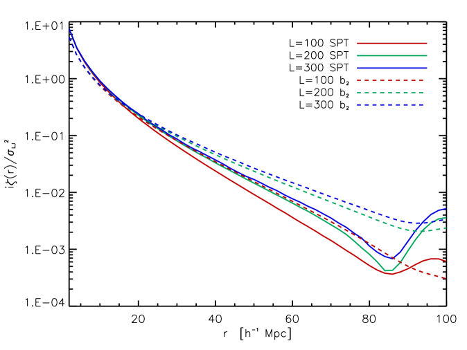
Figure 1 shows the scale-dependencies of $i\zeta_{\rm SPT}$ and $i\zeta_{b_{2}}$ at $z=0$ with $P_{l}(k)$ computed by CLASS [26]. We normalize $i\zeta(r)$ by $\sigma_{L,l}^{2}$, where

$$\sigma_{L,l}^{2}\equiv\langle\bar{\delta}_{l}(\mathbf{r}_{L})^{2}\rangle=\frac{1}{V_{L}^{2}}\int\frac{d^{3}k}{(2\pi)^{3}}~{}P_{l}(k)|W_{L}(\mathbf{k})|^{2}$$ (2.14)

is the variance of the linear density field in the subvolume $V_{L}$. The choice of this normalization will become clear in section 2.4 where we discuss $i\zeta$ in the squeezed limit, i.e., $r\ll L$. We find that the scale-dependencies of $i\zeta_{\rm SPT}(r)$ and $i\zeta_{b_{2}}(r)$ are similar especially on small scales. This is because the scale-dependence of the bispectrum in the squeezed limit is (see e.g. the appendix of ref. [2])

$$B_{\rm SPT}\to\left[\frac{68}{21}-\frac{1}{3}\frac{d\ln k^{3}P_{l}(k)}{d\ln k}\right]P_{l}(k)P_{l}(q)~{},~{}~{}B_{b_{2}}\to 2P_{l}(k)P_{l}(q)~{},$$ (2.15)

where $k$ and $q$ are the short- and long-wavelength modes, respectively. For a power-law power spectrum without features, the squeezed-limit $B_{\rm SPT}$ and $B_{b_{2}}$ have exactly the same scale dependence and cannot be distinguished. This results in a significant residual degeneracy between $b_{1}$ and $b_{2}$, and will be discussed in section 5. When $r$ is small, $i\zeta(r)/\sigma_{L,l}^{2}$ becomes independent of the subvolume size. We derive this feature when we discuss the squeezed limit in section 2.4.

2.3 Connection to the integrated bispectrum

Fourier transforming the density fields, the integrated three-point function can be written as

$$i\zeta(\mathbf{r})\> =\frac{1}{V_{L}^{2}}\int\frac{d^{3}q_{1}}{(2\pi)^{3}}\cdots\int\frac{d^{3}q_{6}}{(2\pi)^{3}}~{}(2\pi)^{9}\delta_{D}(\mathbf{q}_{1}+\mathbf{q}_{2}+\mathbf{q}_{3})\delta_{D}(\mathbf{q}_{1}+\mathbf{q}_{2}+\mathbf{q}_{4}+\mathbf{q}_{5})\delta_{D}(\mathbf{q}_{3}+\mathbf{q}_{6})$$

$$~{}~{}~{}~{}~{}~{}~{}~{}~{}~{}~{}~{}~{}~{}~{}~{}~{}~{}\times B(\mathbf{q}_{1},\mathbf{q}_{2},\mathbf{q}_{3})W_{L}(\mathbf{q}_{4})W_{L}(\mathbf{q}_{5})W_{L}(\mathbf{q}_{6})e^{i[\mathbf{r}\cdot(\mathbf{q}_{1}+\mathbf{q}_{4})-\mathbf{r}_{L}\cdot(\mathbf{q}_{4}+\mathbf{q}_{5}+\mathbf{q}_{6})]}$$

$$=\int\frac{d^{3}k}{(2\pi)^{3}}~{}iB(\mathbf{k})e^{i\mathbf{r}\cdot\mathbf{k}}~{},$$ (2.16)

where $B(\mathbf{q}_{1},\mathbf{q}_{2},\mathbf{q}_{3})$ is the bispectrum of the tracers, and

$$iB(\mathbf{k})\equiv\frac{1}{V_{L}^{2}}\int\frac{d^{3}q_{1}}{(2\pi)^{3}}\int\frac{d^{3}q_{3}}{(2\pi)^{3}}~{}B(\mathbf{k}-\mathbf{q}_{1},-\mathbf{k}+\mathbf{q}_{1}+\mathbf{q}_{3},-\mathbf{q}_{3})W_{L}(\mathbf{q}_{1})W_{L}(-\mathbf{q}_{1}-\mathbf{q}_{3})W_{L}(\mathbf{q}_{3})\,,$$ (2.17)

is the integrated bispectrum as defined in eq. (2.7) of ref. [2]. Eq. (2.16) shows that the integrated three-point function is the Fourier transform of the integrated bispectrum. Similarly, the angle-averaged integrated three-point function is related to the angle-averaged integrated bispectrum, $iB(k)\equiv(4\pi)^{-1}\int{d^{2}\hat{k}}~{}iB(\mathbf{k})$, as

$$i\zeta(r)=\int\frac{k^{2}dk}{2\pi^{2}}~{}iB(k)\,{\rm sinc}(kr)\,.$$ (2.18)

2.4 Squeezed limit

In the squeezed limit, where the separation of the position-dependent correlation function is much smaller than the size of the subvolume ($r\ll L$), the integrated three-point function has a straightforward physical interpretation [2]. In this case, the mean density in the subvolume acts effectively as a constant “background” density. Consider the position-dependent correlation function, $\hat{\xi}(\mathbf{r},\mathbf{r}_{L})$, measured in a subvolume with overdensity $\bar{\delta}(\mathbf{r}_{L})$. If the overdensity is small, we may Taylor expand $\hat{\xi}(\mathbf{r},\mathbf{r}_{L})$ in orders of $\bar{\delta}$ as

$$\hat{\xi}(\mathbf{r},\mathbf{r}_{L})=\left.\xi(\mathbf{r})\right|_{\bar{\delta}=0}+\left.\frac{d\xi(\mathbf{r})}{d\bar{\delta}}\right|_{\bar{\delta}=0}\bar{\delta}+\mathcal{O}(\bar{\delta}^{2})~{}.$$ (2.19)

The integrated three-point function in the squeezed limit is then, at leading order in the variance $\langle\bar{\delta}^{2}\rangle$ (dropping $\bar{\delta}=0$ in the subscript of the derivative term for clarity), given by

$$i\zeta(\mathbf{r})=\langle\hat{\xi}(\mathbf{r},\mathbf{r}_{L})\bar{\delta}(\mathbf{r}_{L})\rangle=\frac{d\xi(\mathbf{r})}{d\bar{\delta}}\langle\bar{\delta}^{2}\rangle+\mathcal{O}(\bar{\delta}^{3})~{}.$$ (2.20)

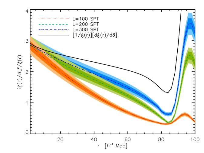
As $\langle\bar{\delta}^{2}\rangle=\sigma_{L}^{2}$, $i\zeta(\mathbf{r})$ normalized by $\sigma_{L}^{2}$ is $d\xi(\mathbf{r})/d\bar{\delta}$ at leading order, which is the linear response of the correlation function to the overdensity. Note that in eq. (2.20) there is no dependence on the subvolume size apart from $\sigma_{L}^{2}$, as shown also by the asymptotic behavior of the solid lines in figure 1 for $r\to 0$.

As $i\zeta(r)$ is the Fourier transform of $iB(k)$, the response of the correlation function, $d\xi(r)/d\bar{\delta}$, is also the Fourier transform of the response of the power spectrum, $dP(k)/d\bar{\delta}$. For example, we can calculate the response of the linear matter correlation function, $d\xi_{l}(r)/d\bar{\delta}$, by Fourier transforming $dP_{l}(k)/d\bar{\delta}=[68/21-(1/3)d\ln k^{3}P_{l}(k)/d\ln k]P_{l}(k)$ [2]. In figure 2, we compare the normalized $i\zeta_{\rm SPT}(r)$ with $d\xi_{l}(r)/d\bar{\delta}$. Due to the large dynamic range of the correlation function, we divide all the predictions by $\xi(r)$. As expected, the smaller the subvolume size, the smaller the $r$ for $i\zeta_{\rm SPT}(r)$ to be close to $[1/\xi_{l}(r)][d\xi_{l}(r)/d\bar{\delta}]$, i.e., reaching the squeezed limit. Specifically, for $100~{}h^{-1}~{}{\rm Mpc}$, $200~{}h^{-1}~{}{\rm Mpc}$, and $300~{}h^{-1}~{}{\rm Mpc}$ subvolumes, the squeezed limit is reached to 10% level at $r\sim 10~{}h^{-1}~{}{\rm Mpc}$, $18~{}h^{-1}~{}{\rm Mpc}$, and $25~{}h^{-1}~{}{\rm Mpc}$, respectively.

Figure 2: The linear response function $[1/\xi_{l}(r)][d\xi_{l}(r)/d\bar{\delta}]$ (black solid) and the normalized $i\zeta_{\rm SPT}(r)$ for $L=100~{}h^{-1}~{}{\rm Mpc}$ (red dotted), $200~{}h^{-1}~{}{\rm Mpc}$ (green dashed), and 300$~{}h^{-1}~{}{\rm Mpc}$ (blue dot-dashed). The light and dark bands correspond to $\pm 5\%$ and $\pm 10\%$ of the predictions, respectively.

2.5 Bispectrum in redshift space

To model $i\zeta(r)$ in redshift space, we need a model for the bispectrum in redshift space. SPT in redshift space at the tree level predicts the halo bispectrum with local bias as [27]

$$B_{z,{\rm tree-level}}(\mathbf{k}_{1},\mathbf{k}_{2},\mathbf{k}_{3})=2[Z_{2}(\mathbf{k}_{1},\mathbf{k}_{2})Z_{1}(\mathbf{k}_{1})Z_{1}(\mathbf{k}_{2})P_{l}(k_{1})P_{l}(k_{2})+2~{}{\rm cyclic}]\,,$$ (2.21)

with

$$Z_{1}(\mathbf{k}_{i})\> =(b_{1}+f\mu_{i}^{2})\,,$$

$$Z_{2}(\mathbf{k}_{1},\mathbf{k}_{2})\> =b_{1}F_{2}(\mathbf{k}_{1},\mathbf{k}_{2})+f\mu^{2}G_{2}(\mathbf{k}_{1},\mathbf{k}_{2})+\frac{f\mu k}{2}\Big{[}\frac{\mu_{1}}{k_{1}}(b_{1}+f\mu_{2}^{2})+\frac{\mu_{2}}{k_{2}}(b_{1}+f\mu_{1}^{2})\Big{]}+\frac{b_{2}}{2}~{},$$ (2.22)

where $F_{2}$ and $G_{2}$ are the standard kernels of SPT [1], $f=d\ln D/d\ln a$ is the logarithmic growth rate, $\mu\equiv\hat{k}\cdot\hat{r}_{\rm los}$, $\mu_{i}\equiv\hat{k}_{i}\cdot\hat{r}_{\rm los}$, and $\mathbf{k}\equiv\mathbf{k}_{1}+\mathbf{k}_{2}$.

The integrated three-point function is the Fourier transform of the integrated bispectrum. Thus, we can evaluate $i\zeta(r)$ by using eq. (2.21) in eq. (2.17) and averaging over the angle of ${\bf k}$ as in eq. (2.18). This operation requires a nine-dimensional integral. On the other hand, if we have an expression for the three-point function in configuration space, such as eq. (2.11), we can use eq. (2.9) to evaluate $i\zeta(r)$, which requires an eight-dimensional integral. We do not always have an analytical expression for the three-point function in configuration space; thus, we in general need to perform the nine-dimensional integral to obtain $i\zeta(r)$ from the bispectrum.

Nevertheless, to check the precision of numerical integration, we compare the results from the eight-dimensional integral in eq. (2.9) with eq. (2.11), and the nine-dimensional integral in eq. (2.17) and eq. (2.18) with $B({\bf k}_{1},{\bf k}_{2},{\bf k}_{3})=2[F_{2}({\bf k}_{1},{\bf k}_{2})P_{l}(k_{1})P_{l}(k_{2})+2~{}\rm{cyclic}]$. As the latter gives a noisy result, we apply a Savitzky-Golay filter (with window size 9 and polynomial order 4) six times. We find that, on the scales of interest ($30~{}h^{-1}~{}{\rm Mpc}\leq r\leq 78~{}h^{-1}~{}{\rm Mpc}$, which we will justify in section 3.3), both results are in agreement to within 2%. We repeat the same test for $i\zeta_{b_{2}}$ (eq. (2.13)), finding a similar result. As the current uncertainty on the measured integrated correlation function presented in this paper is of order 10%, we conclude that our numerical integration yields sufficiently precise results.

2.6 Shot noise

If the density field is traced by discrete particles, $\delta_{d}(\mathbf{r})$, then the three-point function contains a shot noise contribution given by

$$\langle\delta_{d}(\mathbf{r}_{1})\delta_{d}(\mathbf{r}_{2})\delta_{d}(\mathbf{r}_{3})\rangle\> =\langle\delta(\mathbf{r}_{1})\delta(\mathbf{r}_{2})\delta(\mathbf{r}_{3})\rangle$$

$$+\left[\frac{\langle\delta(\mathbf{r}_{1})\delta(\mathbf{r}_{2})\rangle}{\bar{n}(\mathbf{r}_{3})}\delta_{D}(\mathbf{r}_{1}-\mathbf{r}_{3})+2~{}{\rm cyclic}\right]+\frac{\delta_{D}(\mathbf{r}_{1}-\mathbf{r}_{2})\delta_{D}(\mathbf{r}_{1}-\mathbf{r}_{3})}{\bar{n}(\mathbf{r}_{2})\bar{n}(\mathbf{r}_{3})}~{},$$ (2.23)

where $\bar{n}(r)$ is the mean number density of the discrete particles. The shot noise can be safely neglected for the three-point function because it only contributes when $\mathbf{r}_{1}=\mathbf{r}_{2}$, $\mathbf{r}_{1}=\mathbf{r}_{3}$, or $\mathbf{r}_{2}=\mathbf{r}_{3}$. On the other hand, the shot noise of the integrated three-point function can be computed by inserting eq. (2.23) into eq. (2.9), which yields

$$i\zeta_{\rm shot}(r)=\xi(r)\frac{1}{V_{L}^{2}}\int\frac{d^{2}\hat{r}}{4\pi}\int d^{3}x~{}\left[\frac{1}{\bar{n}(\mathbf{x}+\mathbf{r}+\mathbf{r}_{L})}+\frac{1}{\bar{n}(\mathbf{x}+\mathbf{r}_{L})}\right]W_{L}(\mathbf{x}+\mathbf{r})W_{L}(\mathbf{x})~{},$$ (2.24)

where we have assumed $r\neq 0$. If we further assume that the mean number density is constant, then the shot noise of the integrated three-point function can be simplified as

$$i\zeta_{\rm shot}(r)=2\xi(r)\frac{1}{V_{L}\bar{n}}f_{\rm bndry}(r)~{}.$$ (2.25)

For the measurements of PTHalos mock catalogs and the BOSS DR10 CMASS sample, the shot noise is subdominant (less than 7% of the total signal on the scales of interest).

3 Application to PTHalos mock catalogs

Before we apply the position-dependent correlation function technique to the real data, we apply it to the 600 PTHalos mock galaxy catalogs of the BOSS DR10 CMASS sample in the North Galactic Cap (NGC). From now on, we refer to the real and mock BOSS DR10 CMASS samples as the “observations” and “mocks”, respectively.

We use the redshift range of $0.43<z<0.7$, and each realization of mocks contains roughly 400,000 galaxies. We convert the positions of galaxies in RA, DEC, and redshift to comoving distances using the cosmological parameters of the mocks. The mocks have the same observational conditions as the observations, and we correct the observational systematics by weighting each galaxy differently. Specifically, we upweight a galaxy if its nearest neighbor has a redshift failure ($w_{\rm zf}$) or a missing redshift due to a close pair ($w_{\rm cp}$). We further apply weights to correct for the correlation between the number density of the observed galaxies and stellar density ($w_{\rm star}$) and seeing ($w_{\rm see}$). We apply the same weights as done in the analyses of the BOSS collaboration, namely FKP weighting, $w_{\rm FKP}=[1+P_{w}\bar{n}(z){\rm comp}]^{-1}$ [28], where $P_{w}=20000~{}h^{-3}~{}{\rm Mpc}^{3}$, and $\bar{n}(z)$ and “${\rm comp}$” are the expected galaxy number density and the survey completeness, respectively, provided in the catalogs. Therefore, each galaxy is weighted by $w_{\rm BOSS}=(w_{cp}+w_{zf}-1)w_{\rm star}w_{\rm see}w_{\rm FKP}$.

In this section, we present measurements from mocks in real space in section 3.3 and redshift space in section 3.4. The application to the CMASS DR10 sample is the subject of section 4.

3.1 Dividing the subvolumes

We use SDSSPix to pixelize the DR10 survey area. In short, at the lowest resolution (res=1) SDSSPix divides the sphere equally into $n_{x}=36$ longitudinal slices across the hemisphere (at equator each slice is 10 degrees wide), and each slice is divided into $n_{y}=13$ pieces along constant latitudes with equal area. Thus, for res=1 there are $n_{x}\times n_{y}=468$ pixels. In general the total number of pixels is $n_{x}^{\prime}\times n_{y}^{\prime}=({\rm res}~{}n_{x})\times({\rm res}~{}n_{y})=(\rm res)^{2}\times 468$, and in this paper we shall set res=1024. After the pixelization, the $i^{\rm th}$ object (a galaxy or a random sample) has the pixel number $(i_{x},i_{y})$.

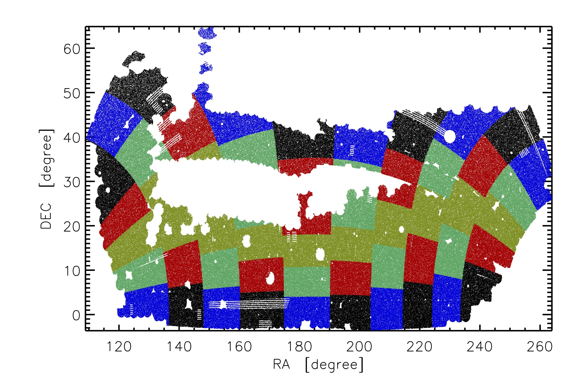
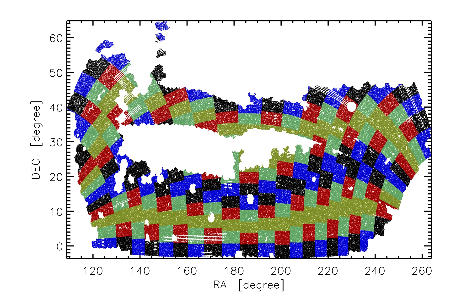
We use two different subvolume sizes. To cut the irregular survey volume into subvolumes with roughly the same size, we first divide the random samples at all redshifts into 10 and 20 slices across longitudes with similar numbers of random samples; we then divide the random samples in each slice into 5 and 10 segments across latitudes with similar numbers of random samples. Figure 3 shows the two resolutions of our subvolumes before the redshift cuts. (Note that this resolution is different from the resolution of SDSSPix, which we always set to res=1024.) Each colored pattern extends over the redshift direction. Finally, we divide the two resolutions into three ($z_{\rm cut}=0.5108$, 0.5717) and five ($z_{\rm cut}=0.48710$, 0.52235, 0.55825, 0.60435) redshift bins.

As a result, there are 150 and 1000 subvolumes for the low and high resolution configurations, respectively. The sizes of the subvolumes are approximately $V_{L}^{1/3}=220~{}h^{-1}~{}{\rm Mpc}$ and $120~{}h^{-1}~{}{\rm Mpc}$, respectively. The fractional differences between the numbers of the random samples in subvolumes for the low and high resolutions are within ${}^{+0.68\%}_{-0.58\%}$ and ${}^{+1.89\%}_{-1.83\%}$, respectively. Since the number of random samples represents the effective volume, all subvolumes at a given resolution have similar effective volumes. We assign galaxies into subvolumes following the division of random samples.

Figure 3: Division of random samples into subvolumes with two resolutions in the RA-DEC plane. Each colored pattern extends over the redshift direction.

3.2 Estimators in the subvolumes

In the $i^{\rm th}$ subvolume, we measure the mean overdensity with respect to the entire NGC, $\bar{\delta}_{i}$, and the position-dependent correlation function, $\hat{\xi}_{i}(r)$. The mean overdensity is estimated by comparing the total weighted galaxies to the expected number density given by the random samples, i.e.,

$$\bar{\delta}_{i}=\frac{1}{\alpha}\frac{w_{g,i}}{w_{r,i}}-1\,,~{}~{}~{}~{}~{}\alpha\equiv\frac{\sum_{i=1}^{N_{s}}w_{g,i}}{\sum_{i=1}^{N_{s}}w_{r,i}}=\frac{w_{g,{\rm tot}}}{w_{r,{\rm tot}}}~{},$$ (3.1)

where $w_{g,i}$ and $w_{r,i}$ are the total weights ($w_{\rm BOSS}$) of galaxies and random samples in the $i^{\rm th}$ subvolume, respectively, and $N_{s}$ is the number of subvolumes.

We use the Landy-Szalay estimator [29] to estimate the position-dependent correlation function as

$$\hat{\xi}_{{\rm LS},i}(r,\mu)=\frac{DD_{i}(r,\mu)}{RR_{i}(r,\mu)}\left(\frac{[\sum_{r}w_{r,i}]^{2}-\sum_{r}w_{r,i}^{2}}{[\sum_{g}w_{g,i}]^{2}-\sum_{g}w_{g,i}^{2}}\right)-\frac{DR_{i}(r,\mu)}{RR_{i}(r,\mu)}\frac{([\sum_{r}w_{r,i}]^{2}-\sum_{r}w_{r,i}^{2})}{\sum_{g}w_{g,i}\sum_{r}w_{r,i}}+1~{},$$ (3.2)

where $DD_{i}(r,\mu)$, $DR_{i}(r,\mu)$, and $RR_{i}(r,\mu)$ are the weighted numbers of galaxy-galaxy, galaxy-random, and random-random pairs within the $i^{\rm th}$ subvolume, respectively, and $\mu$ is the cosine between the line-of-sight vector and the vector connecting galaxy pairs ($\mathbf{r}_{1}-\mathbf{r}_{2}$). The summations such as $\sum_{r}w_{r,i}$ and $\sum_{g}w_{g,i}$ denote the sum over all the random samples and galaxies within the $i^{\rm th}$ subvolume, respectively. The angular average correlation function is then $\hat{\xi}_{{\rm LS},i}(r)=\int_{0}^{1}d\mu~{}\hat{\xi}_{{\rm LS},i}(r,\mu)$.

Eq. (3.2) estimates the correlation function assuming that the density fluctuation is measured relative to the ${\it local}$ mean. However, the position-dependent correlation function defined in section 2 uses the density fluctuation relative to the global mean. These two fluctuations can be related by $\delta_{\rm global}=(1+\bar{\delta})\delta_{\rm local}+\bar{\delta}$ with $\bar{\delta}=\bar{n}_{\rm local}/\bar{n}_{\rm global}-1$. Thus, the position-dependent correlation function, $\hat{\xi}_{i}(r)$, is related to the Landy-Szalay estimator as

$$\hat{\xi}_{i}(r)=(1+\bar{\delta}_{i})^{2}\hat{\xi}_{{\rm LS},i}(r)+\bar{\delta}_{i}^{2}~{}.$$ (3.3)

To compute the average quantities over all subvolumes, we weight by $w_{r,i}$ in the corresponding subvolume. For example, for a given variable $g_{i}$ in the $i^{\rm th}$ subvolume, the average over all subvolumes, $\bar{g}$, is defined by

$$\bar{g}=\frac{1}{w_{r,{\rm tot}}}\sum_{i=1}^{N_{s}}g_{i}w_{r,i}~{}.$$ (3.4)

Since the number of random samples in each subvolume represents the effective volume, the average quantities are effective-volume weighted. Eq. (3.4) assures that the mean of the individual subvolume overdensities is zero,

$$\bar{\delta}=\frac{1}{w_{r,{\rm tot}}}\sum_{i=1}^{N_{s}}\bar{\delta}_{i}w_{r,i}=\frac{1}{w_{r,{\rm tot}}}\sum_{i=1}^{N_{s}}\left[\frac{1}{\alpha}w_{g,i}-w_{r,i}\right]=\frac{\alpha}{\alpha}-1=0~{}.$$ (3.5)

We also confirm that $\bar{\hat{\xi}}(r)$ from eq. (3.3) agrees with the two-point function of all galaxies in the entire survey, on scales smaller than the subvolume size. integrated three-point function in the subvolume of size $L$ as

$$i\zeta(r)=\frac{1}{w_{r,{\rm tot}}}\sum_{i=1}^{N_{s}}\left[\hat{\xi}_{i}(r)\bar{\delta}_{i}-2\bar{\hat{\xi}}(r)\frac{(1+\alpha)}{\alpha}\frac{\sum_{r}w^{2}_{r,i}}{\sum_{r}\bar{n}_{r,i}{\rm comp}_{r,i}w^{2}_{r,i}}\left(\sum_{r}\frac{1}{\bar{n}_{r,i}{\rm comp}_{r,i}}\right)^{-1}\right]w_{r,i}~{},$$ (3.6)

where the second term in the parentheses is the shot noise contribution, and $\bar{n}_{r,i}$ and ${\rm comp}_{r,i}$ are the expected galaxy number density and the survey completeness, respectively, of the random samples. Similarly, we estimate the shot-noise-corrected variance of the fluctuations in the subvolumes of size $L$ as

$$\sigma_{L}^{2}=\frac{1}{w_{r,{\rm tot}}}\sum_{i=1}^{N_{s}}\left[\bar{\delta}_{i}^{2}-\frac{(1+\alpha)}{\alpha}\frac{\sum_{r}w^{2}_{r,i}}{\sum_{r}\bar{n}_{r,i}{\rm comp}_{r,i}w^{2}_{r,i}}\left(\sum_{r}\frac{1}{\bar{n}_{r,i}{\rm comp}_{r,i}}\right)^{-1}\right]w_{r,i}~{},$$ (3.7)

where the second term in the parentheses is the shot noise contribution. We find that the shot noise is subdominant (less than 10%) in both $i\zeta(r)$ and $\sigma_{L}^{2}$.

3.3 Measurements in real space

Figure 4 shows the measurements of the two-point function $\xi(r)$ from the entire survey (top left) and the normalized integrated three-point functions (bottom panels), $i\zeta(r)/\sigma_{L}^{2}$, for the subvolumes of two sizes ($220~{}h^{-1}~{}{\rm Mpc}$ in the bottom-left and $120~{}h^{-1}~{}{\rm Mpc}$ in the bottom-right panels). The gray lines show individual realizations, while the dashed lines show the mean.

Figure 4: (Top left) $\xi(r)$ of the mocks in real space. The gray lines show individual realizations, while the dashed line shows the mean. The black solid line shows the best-fitting model. (Top right) $\chi^{2}$-histogram of the 600 mocks jointly fitting the models to $\xi(r)$ and $i\zeta(r)/\sigma_{L}^{2}$ in real space. The dashed line shows the $\chi^{2}$-distribution with d.o.f.=36. (Bottom left) $i\zeta(r)/\sigma_{L}^{2}$ of the mocks in real space for $220~{}h^{-1}~{}{\rm Mpc}$ subvolumes. (Bottom right) Same as the bottom left panel, but for $120~{}h^{-1}~{}{\rm Mpc}$ subvolumes.

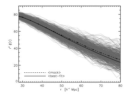
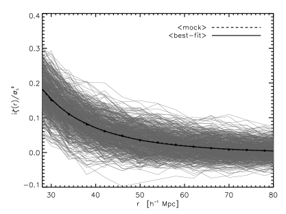
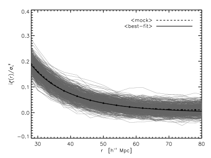
We now fit models of $\xi(r)$ and $i\zeta(r)/\sigma_{L}^{2}$ to the measurements in $30~{}h^{-1}~{}{\rm Mpc}\leq r\leq 78~{}h^{-1}~{}{\rm Mpc}$. We choose this fitting range because there are less galaxy pairs at larger separations due to the subvolume size, and the nonlinear effect becomes too large for our SPT predictions to be applicable at smaller separations. For the two-point function, we take the Fourier transform of [30]

$$P_{g}(k)=b_{1}^{2}[P_{l}(k)e^{-k^{2}\sigma_{v}^{2}}+A_{\rm MC}P_{\rm MC}(k)]~{},$$ (3.8)

where $b_{1}$ is the linear bias, $P_{l}(k)$ is the linear power spectrum, $A_{\rm MC}$ is the mode coupling constant, and

$$P_{\rm MC}(k)=2\int\frac{d^{3}q}{(2\pi)^{3}}~{}P_{l}(q)P_{l}(|\mathbf{k}-\mathbf{q}|)[F_{2}(\mathbf{q},\mathbf{k}-\mathbf{q})]^{2}~{}.$$ (3.9)

Hence, $\xi_{g}(r)=b_{1}^{2}[\xi_{l,\sigma_{v}}(r)+A_{\rm MC}\xi_{\rm MC}(r)]$ with

$$\xi_{l,\sigma_{v}}(r)=\int\frac{d^{3}k}{(2\pi)^{3}}~{}P_{l}(k)e^{-k^{2}\sigma_{v}^{2}}e^{i\mathbf{k}\cdot\mathbf{r}}\,,~{}~{}~{}~{}~{}\xi_{\rm MC}(r)=\int\frac{d^{3}k}{(2\pi)^{3}}~{}P_{\rm MC}(k)e^{i\mathbf{k}\cdot\mathbf{r}}\ .$$ (3.10)

We use a fixed value of $\sigma_{v}^{2}=20.644~{}h^{-2}~{}{\rm Mpc}^{2}$. Varying it has only small effect on the other fitted parameters. For the integrated three-point function, we use the SPT calculation

$$\frac{i\zeta_{g}(r)}{\sigma_{L}^{2}}=\frac{b_{1}i\zeta_{\rm SPT}(r)+b_{2}i\zeta_{b_{2}}(r)}{\sigma_{L,l}^{2}}\frac{1}{f_{\rm bndry}(r)}~{},$$ (3.11)

where $i\zeta_{\rm SPT}(r)$ and $i\zeta_{b_{2}}(r)$ are computed from eq. (2.9) with eqs. (2.11) and (2.13), respectively, and $\sigma_{L,l}^{2}$ is computed from eq. (2.14), using the subvolume sizes of $L=220$ and $120~{}h^{-1}~{}{\rm Mpc}$ and the redshift of $z=0.57$. Note that the size of the subvolumes affects the values of $\sigma_{L,l}^{2}$. We determine $L$ by first measuring $b_{1}^{2}$ using the real-space two-point function of the entire survey, and then find $L$ such that $b_{1}^{2}\sigma_{L,l}^{2}=\sigma_{L}^{2}$ assuming the cubic top-hat window function. We find that these values ($L=220$ and $120~{}h^{-1}~{}{\rm Mpc}$) agree well with the cubic root of the total survey volume divided by the number of subvolumes, to within a few percent.

We fit the models to $\xi(r)$ and $i\zeta(r)/\sigma_{L}^{2}$ of both subvolumes simultaneously by minimizing

$$\chi^{2}=\sum_{ij}C^{-1}_{ij}(D_{i}-M_{i})(D_{j}-M_{j})\,,$$ (3.12)

where $C^{-1}$ is the inverse covariance matrix computed from the 600 mocks, $D_{i}$ and $M_{i}$ are the data and the model in the $i^{\rm th}$ bin, respectively. The models contain three fitting parameters $b_{1}$, $b_{2}$, and $A_{\rm MC}$.

The models computed with the mean of the best-fitting parameters of 600 mocks are shown as the black solid lines in figure 4. The best-fitting parameters are $b_{1}=1.971\pm 0.076$, $b_{2}=0.58\pm 0.31$, and $A_{\rm MC}=1.44\pm 0.93$, where the error bars are 1-$\sigma$ standard deviations. The agreement between the models and the mocks is good, with a difference much smaller than the scatter among 600 mocks. Upon scrutinizing, the difference in $\xi(r)$ is larger for larger separations because the fit is dominated by the small separations with smaller error bars. On the other hand, for $i\zeta(r)/\sigma_{L}^{2}$ the agreement is good for both sizes of subvolumes at all scales of interest. This indicates that the SPT calculation is sufficient to capture the three-point function of the mocks in real space.

The data points in figure 4 are highly correlated. To quantify the quality of the fit, we compute the $\chi^{2}$-histogram from 600 mocks, and compare it with the $\chi^{2}$-distribution with the corresponding degrees of freedom (d.o.f.). There are 13 fitting points for each measurement ($\xi(r)$ and two sizes of subvolumes for $i\zeta(r)/\sigma_{L}^{2}$) and three fitting parameters, so d.o.f.=36. The top right panel of figure 4 shows the $\chi^{2}$-histogram. The dashed line shows the $\chi^{2}$-distribution with d.o.f.=36. The agreement is good, and we conclude that our models well describe both $\xi(r)$ and $i\zeta(r)/\sigma_{L}^{2}$ of the mocks in real space.

Our $b_{1}$ is in good agreement with the results presented in figure 16 of ref. [16], whereas our $b_{2}$ is smaller than theirs, which is $\simeq 0.95$, by 1.2$\sigma$. This may be due to the difference in the bispectrum models. While we restrict to the local bias model and the tree-level bispectrum, ref. [16] includes a non-local tidal bias [31, 32, 33] and uses more sophisticated bispectrum modeling using the effective $F_{2}$ kernel [34, 35]. In appendix B, we show that using the effective $F_{2}$ kernel and the non-local tidal bias in the model increases the value of $b_{2}$, but the changes are well within the 1-$\sigma$ uncertainties. Also, the differences of the goodness of fit for various models are negligible.

The fitting range as well as the shapes of the bispectrum may also affect the results: the integrated correlation function is sensitive only to the squeezed configurations, whereas ref. [16] includes more equilateral and collapsed triangle configurations. Understanding this difference merits further investigations.

3.4 Measurements in redshift space

Figure 5 shows the measurements of $\xi(r)$ (top left) and $i\zeta(r)/\sigma_{L}^{2}$ ($220~{}h^{-1}~{}{\rm Mpc}$ in the bottom-left and $120~{}h^{-1}~{}{\rm Mpc}$ in the bottom-right panels) of the mocks in redshift space. The gray lines show individual realizations, while the dashed lines show the mean. Similar to the analysis in section 3.3, we fit the models in redshift space to the measurements in $30~{}h^{-1}~{}{\rm Mpc}\leq r\leq 78~{}h^{-1}~{}{\rm Mpc}$. In this section, we use General Relativity to compute the growth rate, $f(z)\approx\Omega_{m}(z)^{0.55}$, which yields $f(z=0.57)=0.751$. We shall allow $f$ to vary when interpreting the measurements in the actual data.

Figure 5: Same as figure 4 but in redshift space.

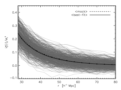
Since there is no baryonic acoustic oscillation feature on the scales we are interested in, we model the redshift-space two-point correlation function as

$$\xi_{g,z}(r)=b_{1}^{2}\left[\xi_{l,\sigma_{v}}(r)+A_{\rm MC}\xi_{\rm MC}(r)\right]K_{p}~{},$$ (3.13)

where $\xi_{l,\sigma_{v}}(r)$ and $\xi_{\rm MC}(r)$ are given in eq. (3.10) and

$$K_{p}\equiv 1+\frac{2}{3}\beta+\frac{1}{5}\beta^{2}~{},$$ (3.14)

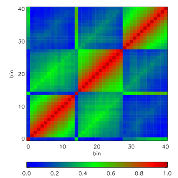
is the Kaiser factor with $\beta\equiv f/b_{1}$ [36]. As we do not include the subdominant term proportional to $b_{2}$ in the two-point function, it only gives a constraint on $b_{1}$, which we can then use to break the degeneracy with $b_{2}$ in the integrated three-point function. We find that this simple modeling yields unbiased $b_{1}$ and fulfills the demand. We calculate the redshift-space normalized integrated three-point function using SPT at the tree level, as described in section 2.5, and then correct for the boundary effect. The $\sigma_{L}^{2}$ of the mocks in redshift space agrees with $b_{1}^{2}K\,\sigma_{L,l}^{2}$ to percent level. The redshift-space models thus contain, as before in real space, the three fitting parameters, $b_{1}$, $b_{2}$, and $A_{\rm MC}$. We then simultaneously fit $\xi(r)$ and $i\zeta(r)/\sigma_{L}^{2}$ of both subvolumes by minimizing eq. (3.12). Figure 6 shows the correlation matrix ($C_{ij}$ in $\chi^{2}$, normalized by $\sqrt{C_{ii}C_{jj}}$) estimated from the 600 mocks in redshift space. Because we normalize the integrated three-point function by $\sigma_{L}^{2}$, the covariance between $i\zeta(r)/\sigma_{L}^{2}$ and $\sigma_{L}^{2}$ is negligible. On the other hand, the covariances between $i\zeta(r)/\sigma_{L}^{2}$ and $\xi(r)$, between $\xi(r)$, and between $i\zeta(r)/\sigma_{L}^{2}$ for two sizes of subvolumes are significant.

Figure 6: Correlation matrix estimated from 600 mocks in redshift space. The figure shows $\sigma_{L}^{2}$ and $i\zeta(r)/\sigma_{L}^{2}$ of $220~{}h^{-1}~{}{\rm Mpc}$ subvolumes from bin 0 to 13, $\sigma_{L}^{2}$ and $i\zeta(r)/\sigma_{L}^{2}$ of $120~{}h^{-1}~{}{\rm Mpc}$ subvolumes from bin 14 to 27, and $\xi(r)$ from bin 28 to 40.

The models computed with the mean of the best-fitting parameters of 600 mocks are shown as the thick solid lines in figure 5. The best-fitting parameters are $b_{1}=1.931\pm 0.077$, $b_{2}=0.54\pm 0.35$, and $A_{\rm MC}=1.37\pm 0.82$. The agreement between the models and the measurements in redshift space is as good as in real space.

Again, our $b_{1}$ is in good agreement with the results presented in figure 16 of ref. [16], whereas our $b_{2}$ is smaller than theirs, which is $\simeq 0.75$, but still well within the 1-$\sigma$ uncertainty. As noted in section 3.3, the adopted models of the bispectrum are different. In appendix B, we show that using the effective $F_{2}$ and $G_{2}$ kernels and the non-local tidal bias in the model increases the value of $b_{2}$. However, the changes are within the uncertainties, and the goodness of the fit is similar for different models. Thus, in this paper we shall primarily use the SPT at the tree level with local bias for simpler interpretation of the three-point function, but also report the results for the extended models.

4 Measurements of the BOSS DR10 CMASS sample

Figure 7: Measurements of the BOSS DR10 CMASS sample (black solid lines). The gray lines show individual mocks in redshift space and the dashed line shows the mean of mocks. (Top left) $\xi(r)$, (Bottom left) $i\zeta(r)/\sigma_{L}^{2}$ for $220~{}h^{-1}~{}{\rm Mpc}$ subvolumes, and (Bottom right) $i\zeta(r)/\sigma_{L}^{2}$ for $120~{}h^{-1}~{}{\rm Mpc}$ subvolumes. (Top right) $\chi^{2}$-histogram of the 600 mocks jointly fitting the three amplitudes to $\xi(r)$ and $i\zeta(r)/\sigma_{L}^{2}$ in redshift space. The dashed line shows the $\chi^{2}$-distribution with d.o.f.=38. The $\chi^{2}$ value measured from the BOSS DR10 CMASS sample is 46.4.

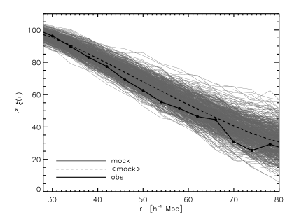
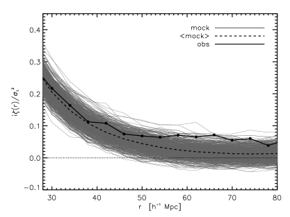
We now present measurements of the position-dependent correlation function from the BOSS DR10 CMASS sample in NGC. The detailed description of the observations can be found in refs. [18, 19]. Briefly, the sample contains 392,372 galaxies over 4,892 deg² in the redshift range of $0.43<z<0.7$, which corresponds to the comoving volume of approximately $2~{}h^{-3}~{}{\rm Gpc}^{3}$. We also weight the galaxies by $w_{\rm BOSS}$ to correct for the observational systematics. We follow section 3.1 to divide the observations into subvolumes. However, the observations have their own set of random samples, which are different from the ones of the mocks (the random samples of the mocks have slightly higher $\bar{n}$ and different $\bar{n}(z)$), so we adjust the redshift cuts to be $z_{\rm cut}=0.5108$, 0.5717 and $z_{\rm cut}=0.48710$, 0.52235, 0.55825, 0.60435 for the two resolutions, respectively. The resulting properties of subvolumes of the observations and mocks are similar.

The mocks are constructed to match the two-point function of the observed galaxies, but not for the three-point function. Hence there is no guarantee that the three-point function of mocks agrees with the observations. We can test this using our measurements.

	avg$[\sigma_{L,\rm mock}^{2}]$	var$[\sigma_{L,\rm mock}^{2}]$	$\sigma_{L,\rm data}^{2}$
$220~{}h^{-1}~{}{\rm Mpc}$	$4.6\times 10^{-3}$	$5.6\times 10^{-4}$	$4.9\times 10^{-3}$
$120~{}h^{-1}~{}{\rm Mpc}$	$2.4\times 10^{-2}$	$1.3\times 10^{-3}$	$2.5\times 10^{-2}$

Table 1: Measurements of $\sigma_{L}^{2}$ of the mock catalogs and the BOSS DR10 CMASS sample.

The measurements of $\xi(r)$ and $i\zeta(r)/\sigma_{L}^{2}$ from the observations are shown as the solid lines in figure 7; the measurements of $\sigma_{L}^{2}$ is summarized in table 1. The measurements are consistent visually with the mocks within the scatter of the mocks, and we shall quantify the goodness of fit using $\chi^{2}$ statistics later.

To quantify statistical significance of the detection of $i\zeta(r)/\sigma_{L}^{2}$ and the goodness of fit, we use the mean of the mocks as the model (instead of the model based on perturbation theory used in section 3.4), and fit only the amplitudes of $i\zeta(r)/\sigma_{L}^{2}$, $\xi(r)$, and $\sigma_{L}^{2}$ to the observations and the 600 mocks by minimizing eq. (3.12). Specifically, we use $O_{i}(r)=A_{i}\,O_{i}^{\rm mock}(r)$ as the model, where $O_{1}(r)=i\zeta(r)/\sigma_{L}^{2}$, $O_{2}(r)=\xi(r)$, and $O_{3}=\sigma_{L}^{2}$, with the amplitudes $A_{1},\,A_{2},\,A_{3}$.

	$A_{1}$	$A_{2}$	$A_{3}$
1-$\sigma$ error	0.12	0.03	0.04
best-fit (DR10)	0.89	1.02	1.08

	$(A_{1},A_{2})$	$(A_{1},A_{3})$	$(A_{2},A_{3})$
corr	0.34	0.09	0.36

Table 2: Results of fitting the amplitudes: $A_{1}$ is $i\zeta(r)/\sigma_{L}^{2}$, $A_{2}$ is $\xi(r)$, and $A_{3}$ is $\sigma_{L}^{2}$. (Left) The 1-$\sigma$ uncertainties of the amplitudes estimated from the mocks, and the best-fitting amplitudes of BOSS DR10 CMASS sample with respect to the mean of the mocks. (Right) The correlation coefficients of the amplitudes.

Table 2 summarizes the fitted amplitudes. The 1-$\sigma$ uncertainties and the correlations are estimated from the 600 mocks. Since we normalize $i\zeta(r)$ by $\sigma_{L}^{2}$, the correlation between $A_{1}$ and $A_{3}$ is small. On the other hand, $A_{2}$ and $A_{3}$ are correlated significantly because $\sigma_{L}^{2}$ is an integral of the two-point function [eq. (2.14)].

Comparing the BOSS DR10 CMASS sample to the mean of the mocks, we find that $i\zeta(r)/\sigma_{L}^{2}$ is 1-$\sigma$ lower, $\xi(r)$ is unbiased (by construction of the mocks), and $\sigma_{L}^{2}$ is 2-$\sigma$ higher. The result of $A_{1}$ for the data is driven by the correlation between different separations of $i\zeta(r)/\sigma_{L}^{2}$. On the other hand, the result of $A_{3}$ is driven by the positive correlation between $\xi(r)$ and $\sigma_{L}^{2}$. While $\sigma_{L}^{2}$ of the data for two subvolumes are larger than that of the mocks but still at the boundary of the variances (see table 1), it requires an even higher $A_{3}$ to minimize $\chi^{2}$ when we jointly fit the three amplitudes. The fact that $A_{3}$ is larger than $A_{2}$ is also possibly due the contributions to $\sigma_{L}^{2}$ from small separations (including stochasticity at zero separations), where the mocks were not optimized. We find $A_{1}=0.89\pm 0.12$, i.e., a 7.4$\sigma$ detection of the integrated three-point function of the BOSS DR10 CMASS sample.

In order to assess the goodness of fit, we use the distribution of $\chi^{2}$, a histogram of which is shown in the top right panel of figure 7. In total there are 41 fitting points (13 fitting points for $\xi(r)$ and two sizes of subvolumes for $i\zeta(r)/\sigma_{L}^{2}$, and two fitting points for $\sigma_{L}^{2}$) with three fitting parameters, so d.o.f.=38. The $\chi^{2}$ value of the observations is 46.4, and the probability to exceed this $\chi^{2}$ value is more than 16%. Given the fact that the mocks are constructed to match only the two-point function of the observations, this level of agreement for both the two-point and integrated three-point correlation functions is satisfactory.

5 Cosmological interpretation of the integrated three-point function

What can we learn from the measured $i\zeta(r)/\sigma_{L}^{2}$? In section 3.4, we show that the prediction for $i\zeta(r)/\sigma_{L}^{2}$ based on SPT at the tree-level in redshift space provides an adequate fit to the mocks to within the scatter of the mocks; thus, we can use this prediction to infer cosmology from $i\zeta(r)/\sigma_{L}^{2}$. Note that any unmodeled effects in the integrated three-point function such as nonlinearities of the matter density, nonlocal bias parameters, and redshift-space distortions beyond the Kaiser factor, will tend to bias our measurement of cosmological parameters based on $i\zeta(r)$. We will discuss caveats at the end of this section.

Since the linear two-point and the tree-level three-point functions are proportional to $\sigma_{8}^{2}$ and $\sigma_{8}^{4}$, respectively, and $\sigma_{L}^{2}$ is proportional to $\sigma_{8}^{2}$, the scaling of the redshift-space correlation functions is

$$\xi_{g,z}(r)\> =b_{1}^{2}K\left[\xi^{\rm fid}_{l,\sigma_{v}}(r)\left(\frac{\sigma_{8}}{\sigma_{8,\rm fid}}\right)^{2}+A_{\rm MC}\xi^{\rm fid}_{\rm MC}(r)\left(\frac{\sigma_{8}}{\sigma_{8,\rm fid}}\right)^{4}\right]\,,$$

$$\frac{i\zeta_{g,z}(r)}{\sigma_{L}^{2}}\> =\frac{i\zeta^{\rm fid}_{g,z}(r)}{b_{1}^{2}\sigma_{L,l}^{2}K_{p}}\left(\frac{\sigma_{8}}{\sigma_{8,\rm fid}}\right)^{2}\frac{1}{f_{\rm bndry}(r)}~{},$$ (5.1)

where “fid” denotes the quantities computed with the fiducial value of $\sigma_{8}$. Note that $\xi_{\rm MC}(r)$ is proportional to $\sigma_{8}^{4}$ because it is an integral of two linear power spectra (see eq. (3.9)). Since $\xi_{l,\sigma_{v}}(r)$ dominates the signal, the parameter combinations $b_{1}\sigma_{8}$ and $K=1+2\beta/3+\beta^{2}/5$ are degenerate in the two-point function. That is, the amplitude of the two-point function measures only $(b_{1}\sigma_{8})^{2}+\frac{2}{3}(b_{1}\sigma_{8})(f\sigma_{8})+\frac{1}{5}(f\sigma_{8})^{2}$. This degeneracy can be lifted by including the quadrupole of the two-point function in redshift space. See refs. [37, 38, 39, 40] for the latest measurements using the BOSS DR11 sample.

As for the three-point function, figure 1 shows that the $b_{1}^{3}$ and $b_{1}^{2}b_{2}$ terms are comparable for $b_{1}\approx b_{2}$. This means that, at the three-point function level, the nonlinear bias appears in the leading order, so the amplitude of the three-point function measures a linear combination of $b_{1}$ and $b_{2}$. This provides a wonderful opportunity to determine $b_{2}$. The challenge is to break the degeneracy between $b_{2}$, $b_{1}$, $f$, and $\sigma_{8}$. For this purpose, we combine our results with the two-point function in redshift space and the weak lensing measurements of BOSS galaxies. We take the constraints on $b_{1}\sigma_{8}(z=0.57)=1.29\pm 0.03$ and $f(z=0.57)\sigma_{8}(z=0.57)=0.441\pm 0.043$ from table 2 in ref. [37]. To further break the degeneracy between $b_{1}$, $f$, and $\sigma_{8}$, we take the constraint on $\sigma_{8}=0.785\pm 0.044$ from ref. [41, 42], where they jointly analyze the clustering and the galaxy-galaxy lensing using the BOSS DR11 CMASS sample and the shape catalog from Canada France Hawaii Telescope Legacy Survey.

We assume Gaussian priors on $b_{1}\sigma_{8}$, $f\sigma_{8}$, and $\sigma_{8}$ with the known covariance between $b_{1}\sigma_{8}$ and $f\sigma_{8}$. The cross-correlation coefficient between $b_{1}\sigma_{8}$ and $f\sigma_{8}$ is $-0.59$, as shown in figure 6 of ref. [37]. We then run the Markov Chain Monte Carlo with the Metropolis-Hastings algorithm to fit the model eq. (5.1) to the observed $i\zeta(r)/\sigma_{L}^{2}$. We find $b_{2}=0.41\pm 0.41$, and the results for the extended models are summarized in table 3.

	baseline	eff kernel	tidal bias	both
$b_{2}$	$0.41\pm 0.41$	$0.51\pm 0.41$	$0.48\pm 0.41$	$0.60\pm 0.41$

Table 3: Best-fitting $b_{2}$ and their uncertainties for BOSS DR10 CMASS sample for the extended models. The detailed description of the extended models is in appendix B.

The value of $b_{2}$ we find is lower than the mean of the mocks, $b_{2}^{\rm mock}=0.54\pm 0.35$. The difference is mainly due to two reasons. First, the amplitude of the integrated three-point function of the observations is lower than that of the mocks by 10% ($A_{1}=0.89\pm 0.12$). Second, the priors from the correlation function and lensing constraint $b_{1}$ to be close to 2.18, which is larger than that of the mocks, $b_{1}^{\rm mock}=1.93$. Thus, it requires a smaller $b_{2}$ to fit the three-point function. The argument is similar for the extended models. Note, however, that the nonlinear bias of the data is still statistically consistent with the mocks.

Let us conclude this section by listing three caveats regarding our cosmological interpretation of the measured integrated three-point function.

1. The models we use, eq. (5.1), are based on tree-level perturbation theory, the lowest order redshift-space distortion treatment, as well as on the local bias parametrization. While this simple model describes the mocks well, as shown in section 3.3 and 3.4, we discuss in appendix B that using the effective $F_{2}$ and $G_{2}$ and the non-local tidal bias brings $b_{2}$ closer to that of ref. [16]. We, however, find similar goodness of fit for various models, and thus we cannot distinguish between these models.

2. Covariances between the integrated three-point function, monopole and quadrupole two-point function, and weak lensing signals are ignored in our treatment. This can and should be improved by performing a joint fit to all the observables.

3. The cosmology is fixed throughout the analysis, except for $f$ and $\sigma_{8}$. In principle, marginalizing over the cosmological parameters is necessary to obtain self-consistent results, although the normalized integrated three-point function is not sensitive to cosmological parameters such as $\Omega_{m}$ as shown in figure 6 of ref. [2].

These caveats need to be addressed in the future work.

6 Conclusions

In this paper, we have reported on the first measurement of the three-point function with the position-dependent correlation function from the SDSS-III BOSS DR10 CMASS sample. The correlation between the position-dependent correlation function measured within subvolumes and the mean overdensities of those subvolumes is robustly detected at 7.4$\sigma$. This correlation measures the integrated three-point function, which is the Fourier transform of the integrated bispectrum introduced in ref. [2], and is sensitive to the bispectrum in the squeezed configurations.

Both the position-dependent correlation function and the mean overdensity are easier to measure than the three-point function. The computational expense for the two-point function is much cheaper than the three-point function estimator using the triplet-counting method. In addition, for a fixed size of the subvolume, the integrated three-point function depends only on one variable (i.e., separation), unlike the full three-point function which depends on three separations. This property allows for a useful compression of information in the three-point function in the squeezed configurations, and makes physical sense because the integrated three-point function measures how the small-scale two-point function, which depends only on the separation, responds to a long-wavelength fluctuation [2]. As there are only a small number of measurement bins, the covariance matrix of the integrated three-point function is easier to estimate than that of the full three-point function from a realistic number of mocks. We have demonstrated this advantage in the paper.

Of course, since this technique measures the three-point function with one long-wavelength mode (mean overdensity in the subvolumes) and two relatively small-wavelength modes (position-dependent correlation function), it is not sensitive to the three-point function of other configurations, which were explored by ref. [16].

We have used the mock galaxy catalogs, which are constructed to match the two-point function of the SDSS-III BOSS DR10 CMASS sample in redshift space, to validate our method and theoretical model. We show that in both real and redshift space, the integrated three-point function of the mocks can be well described by the tree-level SPT model. However, the nonlinear bias which we obtain from the mocks is higher than that reported in ref. [16]. This is possibly due to the differences in the scales and configurations of the three-point function used for the analyses. As discussed in section 5, any unmodeled nonlinear effects in the redshift-space integrated three-point function of CMASS galaxies will tend to bias $b_{2}$, and will bias this parameter differently than the measurement of ref. [16].

Taking the mean of the mocks as the model, and treating the amplitudes of two- and three-point functions as free parameters, we find the best-fit amplitudes of $i\zeta(r)/\sigma_{L}^{2}$, $\xi(r)$, and $\sigma_{L}^{2}$ of the CMASS sample. With respect to the mean of the mocks, the observations show a somewhat smaller $i\zeta(r)/\sigma_{L}^{2}$ ($A_{1}=0.89\pm 0.12$) and larger $\sigma_{L}^{2}$, while the ensemble two-point function $\xi(r)$ matches the mocks. Given that the mocks are generated to match specifically the two-point function of the BOSS DR10 CMASS sample within a certain range of separations, the level of agreement between the observations and mocks is satisfactory.

Finally, by combining the integrated three-point function and the constraints from the anisotropic clustering ($b_{1}\sigma_{8}$ and $f\sigma_{8}$ in [37]) and from the weak lensing measurements ($\sigma_{8}$ in [42]), we break the degeneracy between $b_{1}$, $b_{2}$, $f$, and $\sigma_{8}$. We find $b_{2}=0.41\pm 0.41$ for the BOSS DR10 CMASS sample. The caveat of this result is that our model, eq. (5.1), relies on a rather simple model in redshift space as well as on the local bias parametrization. We leave the extension of the model to improved bias and redshift-space distortion modeling (especially in light of the comparison with the results in ref. [16]) for future work.

In summary, we have demonstrated that the integrated three-point function is a new observable which can be measured straightforwardly from galaxy surveys using basically the existing and routinely applied machinery to compute the two-point function, and has the potential to yield a useful constraint on the quadratic nonlinear bias parameter. Moreover, since the integrated three-point function is most sensitive to the bispectrum in the squeezed configurations, it is sensitive to primordial non-Gaussianity of the local type (parametrized by $f_{\rm NL}$), thereby offering a probe of the physics of inflation. We plan to extend this work to search for the signature of primordial non-Gaussianity in the full BOSS galaxy sample.

Appendix A Testing the integrated three-point function estimator with Gaussian realizations and the local bias model

Figure 8: The normalized integrated three-point functions of the mock halo density field with $b_{1}=3$ and $b_{2}=1$. The left and right panels are for $V_{L}=100~{}h^{-3}~{}{\rm Mpc}^{3}$ and $200~{}h^{-3}~{}{\rm Mpc}^{3}$, respectively. The data points show the mean of 300 Gaussian realizations, and the error bars are the variances of the mean (but note that the data points are highly correlated). The blue dashed and red solid lines are the theoretical models ($i\zeta_{b_{2}}$) without and with $[f_{\rm bndry}(r)]^{-1}$, respectively.

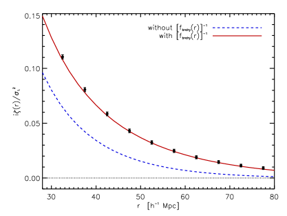
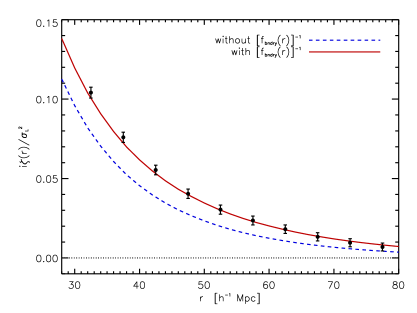
We shall demonstrate that our integrated three-point function estimator is unbiased. To do this, we first generate the matter density field, $\delta_{m}(\mathbf{r})$, by Gaussian realizations with $P_{l}(k)$ at $z=0$ for the volume $V_{r}$ of $1200~{}h^{-3}~{}{\rm Mpc}^{3}$ and a mesh size of $4~{}h^{-1}~{}{\rm Mpc}$. We then compute a mock “halo” density field using the local bias model via

$$\delta_{h}(\mathbf{r})=b_{1}\delta_{m}(\mathbf{r})+\frac{b_{2}}{2}\left[\delta_{m}^{2}(\mathbf{r})-\frac{\sum_{\mathbf{r}\in V_{r}}\delta_{m}^{2}(\mathbf{r})}{\sum_{\mathbf{r}\in V_{r}}1}\right]~{},$$ (A.1)

where we set $b_{1}=3$ and $b_{2}=1$, and $\sum_{\mathbf{r}\in V_{r}}$ denotes a sum over grid cells in the entire volume. Note that $\sum_{\mathbf{r}\in V_{r}}\delta_{h}(\mathbf{r})=0$. We then divide the entire volume $V_{r}$ into $N_{s}=12^{3}=1728$ subvolumes $V_{L}$ of $100~{}h^{-3}~{}{\rm Mpc}^{3}$ and $N_{s}=6^{3}=216$ subvolumes $V_{L}$ of $200~{}h^{-3}~{}{\rm Mpc}^{3}$. The two-point function in the subvolumes and the integrated three-point function are estimated by

$$\xi_{h}(r,\mathbf{r}_{L})=\frac{\sum_{\mathbf{x}+\mathbf{r},\mathbf{x}\in V_{L}}\delta_{h}(\mathbf{x}+\mathbf{r})\delta_{h}(\mathbf{x})}{\sum_{\mathbf{x}+\mathbf{r},\mathbf{x}\in V_{L}}1}~{},~{}~{}i\zeta_{h}(r)=\sum_{i=1}^{N_{s}}\xi_{h}(r,\mathbf{r}_{L})\bar{\delta}_{h}(\mathbf{r}_{L})~{},$$ (A.2)

where $\bar{\delta}_{h}(\mathbf{r}_{L})$ is the mean halo overdensity in the subvolume centered at $\mathbf{r}_{L}$. Note that the denominator in the estimator of $\xi_{h}(r,\mathbf{r}_{L})$ takes the boundary effect into account so $\langle\xi_{h}(r,\mathbf{r}_{L})\rangle=\xi_{h}(r)$ without $f_{\rm bndry}(r)$. This means that the theoretical model of the integrated three-point function computed by eq. (2.9) has to be divided by $f_{\rm bndry}(r)$. Since $\delta_{m}(\mathbf{r})$ is Gaussian, the only contribution to the three-point function is from the nonlinear bias term, and so the estimated integrated three-point function is exactly given by $\frac{i\zeta_{b_{2}}(r)}{f_{\rm bndry}(r)}$.

Figure 8 shows the normalized integrated three-point functions of the mock halo density field with $b_{1}=3$ and $b_{2}=1$ from 300 Gaussian realizations. The measurements are in excellent agreement with $\frac{i\zeta_{b_{2}}(r)}{f_{\rm bndry}(r)}$. This test gives us the confidence that our estimator is unbiased.

Appendix B Effects of effective $F_{2}$ and $G_{2}$ kernels and non-local tidal bias

In this appendix, we show how the inferred value of $b_{2}$ changes when extending our baseline model for the bispectrum based on SPT at the tree level with local bias to the model used in the analysis of ref. [16].

Their model replaces $F_{2}$ and $G_{2}$ in eq. (2.21) with “effective” kernels, $F_{2}^{\rm eff}$ [34] and $G_{2}^{\rm eff}$ [35], which are calibrated to match the nonlinear matter bispectrum in of N-body simulations. Their model also adds a non-local galaxy bias caused by tidal fields [31, 32, 33] to $Z_{2}$, i.e., $Z_{2}\to Z_{2}+\frac{1}{2}b_{s^{2}}\left[(\hat{k}_{1}\cdot\hat{k}_{2})^{2}-\frac{1}{3}\right]$, where $b_{s^{2}}=-(4/7)(b_{1}-1)$. We use this model to compute the integrated three-point function, and find $b_{2}$ of the mocks in real and redshift space by performing a joint fit with the two-point function as described in section 3.3 and 3.4.

r-space	$b_{1}$	$b_{2}$
baseline	$1.971\pm 0.076$	$0.58\pm 0.31$
eff kernel	$1.973\pm 0.076$	$0.62\pm 0.31$
tidal bias	$1.971\pm 0.076$	$0.64\pm 0.31$
both	$1.973\pm 0.076$	$0.68\pm 0.31$

z-space	$b_{1}$	$b_{2}$
baseline	$1.931\pm 0.077$	$0.54\pm 0.35$
eff kernel	$1.933\pm 0.077$	$0.65\pm 0.35$
tidal bias	$1.932\pm 0.077$	$0.60\pm 0.35$
both	$1.933\pm 0.077$	$0.71\pm 0.35$

Table 4: Best-fitting values of $b_{1}$ and $b_{2}$ and their uncertainties for mock catalogs, obtained using different models of the bispectrum in real space (left) and redshift space (right).

Table 4 summarizes the results. The “baseline model” refers to the model based on SPT and local bias. The “eff kernel” refers to the model with $F^{\rm eff}_{2}$, $G^{\rm eff}_{2}$, and local bias. The “tidal bias” refers to the model with $F_{2}$, $G_{2}$, local bias, and tidal bias. Finally, “both” refers to the model with $F^{\rm eff}_{2}$, $G^{\rm eff}_{2}$, local bias, and tidal bias.

Both the effective kernels and the non-local tidal bias result in a larger nonlinear bias, which is in better agreement with ref. [16]. The changes of the best-fitting nonlinear bias, however, are still within the $1-\sigma$ uncertainties, and all the results are consistent with ref. [16]. We also calculate the goodness of the fit for all the models in both real and redshift space by comparing the mean of the mocks and the best-fitting models, as well as the $\chi^{2}$-distribution. We find that all models perform equally well; thus, in this paper we shall primarily use the simplest model, i.e. the SPT at the tree level with local bias for modeling the three-point function, but also report the results for the extended models.

Appendix C Comparison of $i\zeta(r)/\sigma_{L}^{2}$ of BOSS DR10 CMASS sample and PTHalos mock catalogs in different redshift bins

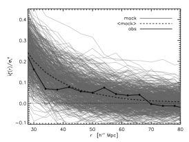
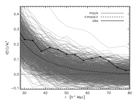
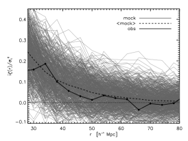
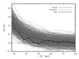
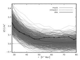
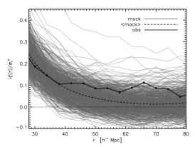
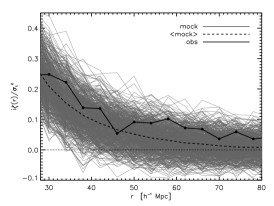
The BOSS DR10 CMASS sample and the mocks have different sets of random samples with slightly different $\bar{n}(z)$, hence the properties of the observations and the mocks may not agree well in all redshift bins. Moreover, as mentioned in ref. [42], the CMASS sample is flux-limited, and thus the observed galaxies statistically have larger stellar masses at higher redshift (see figure 1 in ref. [42]). This may cause redshift evolution of the bias, and so the correlation functions. We shall measure $i\zeta(r)/\sigma_{L}^{2}$ as a function of redshift to test this.

The measurements in the subvolumes are mostly the same as introduced in section 3.2, except that we now measure $\alpha(z_{j})$ as a function of redshift bin $z_{j}$, and the average is done in the individual redshift bin. Namely,

$$\alpha(z_{j})=\frac{\sum_{i\in z_{j}}w_{g,i}}{\sum_{i\in z_{j}}w_{r,i}}=\frac{w_{r,z_{j}}}{w_{g,z_{j}}}\,,~{}~{}~{}~{}~{}\bar{g}(z_{j})=\frac{1}{w_{r,z_{j}}}\sum_{i\in z_{j}}g_{i}w_{r,i}~{}.$$ (C.1)

This assures that $\bar{\delta}(z_{j})=0$ for all redshift bins.

Figure 9 and figure 10 show $i\zeta(r)/\sigma_{L}^{2}$ at different redshift bins for 220 and $120~{}h^{-1}~{}{\rm Mpc}$ subvolumes, respectively. We find no clear sign that $i\zeta(r)/\sigma_{L}^{2}$ of the observations has different redshift evolution relative to the mocks. Thus, it is justified to study $i\zeta(r)/\sigma_{L}^{2}$ using one effective redshift for the BOSS DR10 CMASS sample. With the upcoming DR12 sample with a larger volume, the redshift evolution of $i\zeta(r)/\sigma_{L}^{2}$ can be better studied.

Figure 9: $i\zeta(r)/\sigma_{L}^{2}$ of $220~{}h^{-1}~{}{\rm Mpc}$ subvolumes in different redshift bins. The redshift bins increase from left to right, with the redshift cuts quoted in the beginning of section 3 and 4.

Figure 10: Same as figure 9, but for $120~{}h^{-1}~{}{\rm Mpc}$ subvolumes. The redshift bins increase from top left to bottom right.

Appendix D Fisher matrix of the position-dependent power spectrum

In this appendix we demonstrate that the position-dependent correlation function technique captures the information of the squeezed-limit bispectrum. To this end we utilize the local type of primordial non-Gaussianity, which peaks in the squeezed limit, and show that the full bispectrum and the position-dependent correlation function would yield comparable constraints on $f_{\rm NL}$. As shown in section 2.3, the integrated three-point function is the Fourier transform of the integrated bispectrum. Here we shall compute the Fisher matrix of the integrated bispectrum instead of the integrated three-point function. This simplifies the computation as in this case we may assume the covariance matrix to be diagonal (in the Gaussian limit).

As the main goal of this appendix is to show that the information of the squeezed-limit bispectrum is captured by the position-dependent correlation function technique, we shall use the simplest model for the galaxy bispectrum in the presence of local-type primordial non-Gaussianity and redshift-space distortion. Thus, the galaxy bispectrum is given by

$$B_{g}(\mathbf{k}_{1},\mathbf{k}_{2},vk_{3})=K_{b}\left[b_{1}^{3}B_{\rm SPT}(\mathbf{k}_{1},\mathbf{k}_{2},\mathbf{k}_{3})+b_{1}^{2}b_{2}B_{b_{2}}(\mathbf{k}_{1},\mathbf{k}_{2},\mathbf{k}_{3})+b_{1}^{3}f_{\rm NL}B_{f_{\rm NL}}(\mathbf{k}_{1},\mathbf{k}_{2},\mathbf{k}_{3})\right]~{},$$ (D.1)

where $K_{b}=1+\frac{2}{3}\beta+\frac{1}{9}\beta^{2}$ is the Kaiser factor of the bispectrum and $\beta=f/b_{1}$ [36], and $f_{\rm NL}$ parametrizes the amplitude of the primordial non-Gaussianity. The exact forms of the bispectra are

$$B_{\rm SPT}(\mathbf{k}_{1},\mathbf{k}_{2},\mathbf{k}_{3})\> =2F_{2}(\mathbf{k}_{1},\mathbf{k}_{2})P_{l}(k_{1},a)P_{l}(k_{2},a)+2~{}{\rm cyclic}$$

$$B_{b_{2}}(\mathbf{k}_{1},\mathbf{k}_{2},\mathbf{k}_{3})\> =P_{l}(k_{1},a)P_{2}(k_{2},a)+2~{}{\rm cyclic}$$

$$B_{f_{\rm NL}}(\mathbf{k}_{1},\mathbf{k}_{2},\mathbf{k}_{3})\> =2M(k_{1},a)M(k_{2},a)M(k_{3},a)\left[P_{\Phi}(k_{1})P_{\Phi}(k_{2})+2~{}{\rm cyclic}\right]~{},$$ (D.2)

where $a$ is the scale factor, $M(k,a)=\frac{2}{3}\frac{D(a)}{H_{0}^{2}\Omega_{m}}k^{2}T(k)$ and $T(k)$ is the transfer function, and $P_{\Phi}(k)$ is the power spectrum of the scalar potential. $B_{f_{\rm NL}}$ is produced by the local-type non-Gaussianity in the primordial scalar potential, $\Phi(r)=\phi(r)+f_{\rm NL}\left[\phi^{2}(r)-\langle\phi^{2}(r)\rangle\right]$ where $\phi(r)$ follows the Gaussian statistics [43]. Note that we ignore the effect of the scale-dependent bias due to the local-type primordial non-Gaussianity [44, 45, 46], and the more complete model can be found in [47, 48].

The Fisher matrix of the reduced bispectrum $Q(k_{1},k_{2},k_{3})=B(k_{1},k_{2},k_{3})/[P(k_{1})P(k_{2})+2~{}{\rm cyclic}]$ is given by [49]

$$F_{Q,\alpha\beta}=\sum_{k_{1},k_{2},k_{3}\leq k_{\rm max}}\frac{\partial Q(k_{1},k_{2},k_{3})}{\partial p_{\alpha}}\frac{\partial Q(k_{1},k_{2},k_{3})}{\partial p_{\beta}}\frac{1}{\Delta Q^{2}(k_{1},k_{2},k_{3})}~{},$$ (D.3)

where $(k_{1},k_{2},k_{3})$ have to form a triangle, $p_{\alpha}\in[b_{1},b_{2},f_{\rm NL}]$ are the parameters, and $\Delta Q^{2}(k_{1},k_{2},k_{3})$ is the variance of the reduced bispectrum. Similarly, the Fisher matrix of the normalized integrated bispectrum $ib(k)=iB(k)/[P(k)\sigma_{L}^{2}]$ is given by

$$F_{ib,\alpha\beta}=\sum_{L}\sum_{k\leq k_{\rm max}}\frac{\partial ib(k)}{\partial p_{\alpha}}\frac{\partial ib(k)}{\partial p_{\beta}}\frac{1}{\Delta ib^{2}(k)}~{},$$ (D.4)

where $L$ is the subvolume size and $\Delta ib^{2}(k)$ is the variance of the normalized integrated bispectrum. Note that we assume the Gaussian limit in eqs. (D.3)–(D.4), hence only the diagonal elements of $Q$ and $ib$ exist. Namely, for $Q$, it requires $k_{i}=k_{i}^{\prime}$ for $\langle Q(k_{1},k_{2},k_{3})Q(k_{1}^{\prime},k_{2}^{\prime},k_{3}^{\prime})\rangle$; similarly, for $ib$, it requires $L=L^{\prime}$ and $k=k^{\prime}$. This approximation holds well at high redshift, but would break down at low redshift due to the nonlinear evolution.

To compute the variances, we assume that the dominant component is from the bispectrum in the numerator (instead of the normalization in the denominator). We thus have

$$\Delta Q^{2}(k_{1},k_{2},k_{3})\approx\> \frac{\pi s_{123}}{k_{1}k_{2}k_{3}}\frac{[P_{z}(k_{1})+P_{\rm shot}][P_{z}(k_{2})+P_{\rm shot}][P_{z}(k_{3})+P_{\rm shot}]}{[P_{z}(k_{1})P_{z}(k_{2})+{\rm 2~{}cyclic}]^{2}}~{},$$

$$\Delta ib^{2}(k)\approx\> \frac{V_{L}}{V_{r}N_{kL}}\frac{[\sigma_{L,z}^{2}+P_{\rm shot}/V_{L}][P_{z}(k)+P_{\rm shot}]^{2}}{\sigma_{L,z}^{4}P_{z}^{2}(k)}~{},$$ (D.5)

where $s_{123}=6$, 2, 1 for equilateral, isosceles, and general triangles, respectively, $P_{z}(k)=K_{p}b_{1}^{2}P_{l}(k)$ is the redshift-space power spectrum, $P_{\rm shot}$ is the shot noise of the power spectrum, $N_{kL}$ is the number of independent Fourier modes in the subvolume, and $\sigma_{L,z}^{2}=K_{p}b_{1}^{2}\sigma_{L,l}^{2}$.

Figure 11: Two-dimensional joint 95% C.L. constraints on galaxy biases and primordial non-Gaussianity for BOSS full survey. The survey parameters are in the top right panel. The top-left, bottom-left, and bottom-right panels show the joint constraints on $(b_{1},b_{2})$, $(b_{1},f_{\rm NL})$, and $(b_{2},f_{\rm NL})$ marginalized over $f_{\rm NL}$, $b_{2}$, and $b_{1}$, respectively. The blue dashed, green solid, and red dot-dashed line are for reduced bispectrum with $k_{\rm min}=2\pi/V_{r}^{1/3}$, reduced bispectrum with $k_{\rm min}=2\pi/V_{L}^{1/3}$ where $V_{L}$ is the largest subvolume, and normalized integrated bispectrum for six sizes of subvolumes (100 to $600~{}h^{-1}~{}{\rm Mpc}$ with an increment of $100~{}h^{-1}~{}{\rm Mpc}$), respectively.

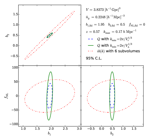
Figure 11 shows the two-dimensional joint 95% C.L. constraints on galaxy biases and primordial non-Gaussianity for the full BOSS survey. One finds that as long as $k_{\rm min}$ is set to be the fundamental frequency of the largest subvolume, the integrated bispectrum technique gives the similar constraint on $f_{\rm NL}$ compared to the full bispectrum analysis. This means that the integrated bispectrum is sensitive to the bispectrum in the squeezed-limit configurations. On the other hand, the top-left panel shows the strong degeneracy between $b_{1}$ and $b_{2}$ for the integrated bispectrum. As discussed in section 2.2, in the squeezed limit $B_{\rm SPT}$ and $B_{b_{2}}$ has the same scale-dependency if the power spectrum is pure power-law. Therefore, if only the squeezed-limit bispectrum is used, such as the integrated bispectrum technique, then it is challenging to break the degeneracy.

We also find that while both techniques give similar constraints on $f_{\rm NL}$, the number of counted Fourier modes differ dramatically. Specifically, the full bispectrum using $k_{\rm min}=2\pi/V_{r}^{1/3}$ and $2\pi/V_{L}^{1/3}$ counts 7113 and 6730 triangles, respectively, while the integrated bispectrum counts only 54 Fourier modes. This means that many of the triangles contain information other than the squeezed configurations and thus the integrated bispectrum can be regarded as an efficient approach to extract the information of the squeezed-limit bispectrum, such as the local-type primordial non-Gaussianity.

References

- [1] F. Bernardeau, S. Colombi, E. Gaztanaga, and R. Scoccimarro, Large scale structure of the universe and cosmological perturbation theory, Phys.Rept. 367 (2002) 1–248, [astro-ph/0112551].
- [2] C.-T. Chiang, C. Wagner, F. Schmidt, and E. Komatsu, Position-dependent power spectrum of the large-scale structure: a novel method to measure the squeezed-limit bispectrum, JCAP 1405 (2014) 048, [arXiv:1403.3411].
- [3] C. Wagner, F. Schmidt, C.-T. Chiang, and E. Komatsu, Separate Universe Simulations, Mon.Not.Roy.Astron.Soc. 448 (2015) 11, [arXiv:1409.6294].
- [4] C. Wagner, F. Schmidt, C.-T. Chiang, and E. Komatsu, The angle-averaged squeezed limit of nonlinear matter N-point functions, arXiv:1503.0348.
- [5] S. Cole and N. Kaiser, Biased clustering in the cold dark matter cosmogony, Mon.Not.Roy.Astron.Soc. 237 (1989) 1127–1146.
- [6] H. Mo and S. D. White, An Analytic model for the spatial clustering of dark matter halos, Mon.Not.Roy.Astron.Soc. 282 (1996) 347, [astro-ph/9512127].
- [7] B. F. Roukema, T. Buchert, J. J. Ostrowski, and M. J. France, Evidence for an environment-dependent shift in the baryon acoustic oscillation peak, Mon.Not.Roy.Astron.Soc. 448 (2015) 1660, [arXiv:1410.1687].
- [8] C.-T. Chiang, P. Wullstein, D. Jeong, E. Komatsu, G. A. Blanc, et al., Galaxy redshift surveys with sparse sampling, JCAP 1312 (2013) 030, [arXiv:1306.4157].
- [9] R. Scoccimarro, H. A. Feldman, J. N. Fry, and J. A. Frieman, The Bispectrum of IRAS redshift catalogs, Astrophys.J. 546 (2001) 652, [astro-ph/0004087].
- [10] L. Verde, A. F. Heavens, W. J. Percival, S. Matarrese, C. M. Baugh, et al., The 2dF Galaxy Redshift Survey: The Bias of galaxies and the density of the Universe, Mon.Not.Roy.Astron.Soc. 335 (2002) 432, [astro-ph/0112161].
- [11] SDSS Collaboration, I. Kayo et al., Three - point correlation functions of SDSS galaxies in redshift space: Morphology, color and luminosity dependence, Publ.Astron.Soc.Jap. 56 (2004) 415, [astro-ph/0403638].
- [12] T. Nishimichi, I. Kayo, C. Hikage, K. Yahata, A. Taruya, et al., Bispectrum and Nonlinear Biasing of Galaxies: Perturbation Analysis, Numerical Simulation and SDSS Galaxy Clustering, Publ.Astron.Soc.Jap. 59 (2007) 93, [astro-ph/0609740].
- [13] C. K. McBride, A. J. Connolly, J. P. Gardner, R. Scranton, J. A. Newman, et al., Three-Point Correlation Functions of SDSS Galaxies: Luminosity and Color Dependence in Redshift and Projected Space, Astrophys.J. 726 (2011) 13, [arXiv:1007.2414].
- [14] C. K. McBride, A. J. Connolly, J. P. Gardner, R. Scranton, R. Scoccimarro, et al., Three-Point Correlation Functions of SDSS Galaxies: Constraining Galaxy-Mass Bias, Astrophys.J. 739 (2011) 85, [arXiv:1012.3462].
- [15] WiggleZ Collaboration Collaboration, F. A. Marin et al., The WiggleZ Dark Energy Survey: constraining galaxy bias and cosmic growth with 3-point correlation functions, Mon.Not.Roy.Astron.Soc. 432 (2013) 2654, [arXiv:1303.6644].
- [16] H. Gil-Marín, J. Noreña, L. Verde, W. J. Percival, C. Wagner, et al., The power spectrum and bispectrum of SDSS DR11 BOSS galaxies I: bias and gravity, arXiv:1407.5668.
- [17] H. Guo, Z. Zheng, Y. Jing, I. Zehavi, C. Li, et al., Modelling The Redshift-Space Three-Point Correlation Function in SDSS-III, Mon.Not.Roy.Astron.Soc. 449 (2015) L95, [arXiv:1409.7389].
- [18] SDSS Collaboration Collaboration, C. P. Ahn et al., The Tenth Data Release of the Sloan Digital Sky Survey: First Spectroscopic Data from the SDSS-III Apache Point Observatory Galactic Evolution Experiment, Astrophys.J.Suppl. 211 (2014) 17, [arXiv:1307.7735].
- [19] BOSS Collaboration, L. Anderson et al., The clustering of galaxies in the SDSS-III Baryon Oscillation Spectroscopic Survey: Baryon Acoustic Oscillations in the Data Release 10 and 11 galaxy samples, Mon.Not.Roy.Astron.Soc. 441 (2014) 24–62, [arXiv:1312.4877].
- [20] R. Scoccimarro and R. K. Sheth, PTHalos: A Fast method for generating mock galaxy distributions, Mon.Not.Roy.Astron.Soc. 329 (2002) 629–640, [astro-ph/0106120].
- [21] M. Manera, R. Scoccimarro, W. J. Percival, L. Samushia, C. K. McBride, et al., The clustering of galaxies in the SDSS-III Baryon Oscillation Spectroscopic Survey: a large sample of mock galaxy catalogues, Mon.Not.Roy.Astron.Soc. 428 (2012), no. 2 1036–1054, [arXiv:1203.6609].
- [22] M. Manera, L. Samushia, R. Tojeiro, C. Howlett, A. J. Ross, et al., The clustering of galaxies in the SDSS-III Baryon Oscillation Spectroscopic Survey: mock galaxy catalogues for the low-redshift sample, Mon.Not.Roy.Astron.Soc. 447 (2015) 437, [arXiv:1401.4171].
- [23] Y. Jing and G. Borner, Three point correlation function in the quasilinear regime, Astron.Astrophys. 318 (1997) 667–672, [astro-ph/9606122].
- [24] J. Barriga and E. Gaztanaga, The 3-point function in the large scale structure. 1. the weakly nonlinear regime in n-body simulations, Mon.Not.Roy.Astron.Soc. 333 (2002) 443–453, [astro-ph/0112278].
- [25] J. N. Fry and E. Gaztanaga, Biasing and hierarchical statistics in large scale structure, Astrophys.J. 413 (1993) 447–452, [astro-ph/9302009].
- [26] J. Lesgourgues, The Cosmic Linear Anisotropy Solving System (CLASS) I: Overview, arXiv:1104.2932.
- [27] R. Scoccimarro, H. Couchman, and J. A. Frieman, The Bispectrum as a signature of gravitational instability in redshift-space, Astrophys.J. 517 (1999) 531–540, [astro-ph/9808305].
- [28] H. A. Feldman, N. Kaiser, and J. A. Peacock, Power spectrum analysis of three-dimensional redshift surveys, Astrophys.J. 426 (1994) 23–37, [astro-ph/9304022].
- [29] S. D. Landy and A. S. Szalay, Bias and variance of angular correlation functions, Astrophys.J. 412 (1993) 64.
- [30] M. Crocce and R. Scoccimarro, Nonlinear Evolution of Baryon Acoustic Oscillations, Phys.Rev. D77 (2008) 023533, [arXiv:0704.2783].
- [31] P. McDonald and A. Roy, Clustering of dark matter tracers: generalizing bias for the coming era of precision LSS, JCAP 0908 (2009) 020, [arXiv:0902.0991].
- [32] T. Baldauf, U. Seljak, V. Desjacques, and P. McDonald, Evidence for Quadratic Tidal Tensor Bias from the Halo Bispectrum, Phys.Rev. D86 (2012) 083540, [arXiv:1201.4827].
- [33] R. K. Sheth, K. C. Chan, and R. Scoccimarro, Nonlocal Lagrangian bias, Phys.Rev. D87 (2013), no. 8 083002, [arXiv:1207.7117].
- [34] H. Gil-Marín, C. Wagner, F. Fragkoudi, R. Jimenez, and L. Verde, An improved fitting formula for the dark matter bispectrum, JCAP 1202 (2012) 047, [arXiv:1111.4477].
- [35] H. Gil-Marín, C. Wagner, J. Noreña, L. Verde, and W. Percival, Dark matter and halo bispectrum in redshift space: theory and applications, JCAP 1412 (2014), no. 12 029, [arXiv:1407.1836].
- [36] N. Kaiser, Clustering in real space and in redshift space, Mon.Not.Roy.Astron.Soc. 227 (1987) 1–27.
- [37] L. Samushia, B. A. Reid, M. White, W. J. Percival, A. J. Cuesta, et al., The Clustering of Galaxies in the SDSS-III Baryon Oscillation Spectroscopic Survey (BOSS): measuring growth rate and geometry with anisotropic clustering, Mon.Not.Roy.Astron.Soc. 439 (2014) 3504–3519, [arXiv:1312.4899].
- [38] R. Tojeiro, A. J. Ross, A. Burden, L. Samushia, M. Manera, et al., The clustering of galaxies in the SDSS-III Baryon Oscillation Spectroscopic Survey: galaxy clustering measurements in the low redshift sample of Data Release 11, Mon.Not.Roy.Astron.Soc. 440 (2014) 2222, [arXiv:1401.1768].
- [39] A. G. Sanchez, F. Montesano, E. A. Kazin, E. Aubourg, F. Beutler, et al., The clustering of galaxies in the SDSS-III Baryon Oscillation Spectroscopic Survey: cosmological implications of the full shape of the clustering wedges, Mon.Not.Roy.Astron.Soc. 433 (2013) 1202–1222, [arXiv:1312.4854].
- [40] BOSS Collaboration Collaboration, F. Beutler et al., The clustering of galaxies in the SDSS-III Baryon Oscillation Spectroscopic Survey: Testing gravity with redshift-space distortions using the power spectrum multipoles, Mon.Not.Roy.Astron.Soc. 443 (2014) 1065, [arXiv:1312.4611].
- [41] H. Miyatake, S. More, R. Mandelbaum, M. Takada, D. N. Spergel, et al., The Weak Lensing Signal and Clustering of SDSS-III CMASS Galaxies I: Measurements, arXiv:1311.1480.
- [42] S. More, H. Miyatake, R. Mandelbaum, M. Takada, D. Spergel, et al., The Weak Lensing Signal and the Clustering of BOSS Galaxies: Astrophysical and Cosmological Constraints, arXiv:1407.1856.
- [43] E. Komatsu and D. N. Spergel, Acoustic signatures in the primary microwave background bispectrum, Phys.Rev. D63 (2001) 063002, [astro-ph/0005036].
- [44] N. Dalal, O. Dore, D. Huterer, and A. Shirokov, The imprints of primordial non-gaussianities on large-scale structure: scale dependent bias and abundance of virialized objects, Phys.Rev. D77 (2008) 123514, [arXiv:0710.4560].
- [45] S. Matarrese and L. Verde, The effect of primordial non-Gaussianity on halo bias, Astrophys.J. 677 (2008) L77–L80, [arXiv:0801.4826].
- [46] A. Slosar, C. Hirata, U. Seljak, S. Ho, and N. Padmanabhan, Constraints on local primordial non-Gaussianity from large scale structure, JCAP 0808 (2008) 031, [arXiv:0805.3580].
- [47] T. Baldauf, U. Seljak, and L. Senatore, Primordial non-Gaussianity in the Bispectrum of the Halo Density Field, JCAP 1104 (2011) 006, [arXiv:1011.1513].
- [48] G. Tasinato, M. Tellarini, A. J. Ross, and D. Wands, Primordial non-Gaussianity in the bispectra of large-scale structure, JCAP 1403 (2014) 032, [arXiv:1310.7482].
- [49] E. Sefusatti and E. Komatsu, The bispectrum of galaxies from high-redshift galaxy surveys: Primordial non-Gaussianity and non-linear galaxy bias, Phys.Rev. D76 (2007) 083004, [arXiv:0705.0343].