Galaxy formation in the Planck Cosmology - III. The high-redshift universe

Abstract

We present high-redshift predictions of the star formation rate distribution function (SFR DF), UV luminosity function (UV LF), galactic stellar mass function (GSMF), and specific star-formation rates (sSFRs) of galaxies from the latest version of the Munich semi-analytic model L-Galaxies. We find a good fit to both the shape and normalisation of the SFR DF at $z=4-7$, apart from a slight under-prediction at the low SFR end at $z=4$. Likewise, we find a good fit to the faint number counts for the observed UV LF; at brighter magnitudes our predictions lie below the observations, increasingly so at higher redshifts. At all redshifts and magnitudes, the raw (unattenuated) number counts for the UV LF lie above the observations. Because of the good agreement with the SFR we interpret our under-prediction as an over-estimate of the amount of dust in the model for the brightest galaxies, especially at high-redshift. While the shape of our GSMF matches that of the observations, we lie between (conflicting) observations at $z=4-5$, and under-predict at $z=6-7$. The sSFRs of our model galaxies show the observed trend of increasing normalisation with redshift, but do not reproduce the observed mass dependence.Overall, we conclude that the latest version of L-Galaxies, which is tuned to match observations at $z\leq 3$, does a fair job of reproducing the observed properties of galaxies at $z\geq 4$. More work needs to be done on understanding observational bias at high-redshift, and upon the dust model, before strong conclusions can be drawn on how to interpret remaining discrepancies between the model and observations.

1 Introduction

With the installation of Wide Field Camera 3 (WFC3) on the Hubble Space Telescope (HST) in 2009 it is now possible to identify statistically useful and robust samples of star forming galaxies in the early Universe ($z>4$, Oesch et al., 2010; Bouwens et al., 2010a; Bunker et al., 2010; Wilkins et al., 2010; Finkelstein et al., 2010; McLure et al., 2010; Wilkins et al., 2011a; Lorenzoni et al., 2011; Bouwens et al., 2011; McLure et al., 2011; Finkelstein et al., 2012a; Lorenzoni et al., 2013; McLure et al., 2013; Duncan et al., 2014; Finkelstein et al., 2014). In recent years a tremendous effort has been dedicated to quantifying the photometric and physical properties, such as star formation rates and stellar masses, of these galaxies. As we continue to dig deeper, with the first sources now identified at $z\approx 10$ (e.g. Oesch et al., 2012; Ellis et al., 2013), and with the launch of the James Webb Space Telescope (JWST) in the next few years, we will further be able to constrain the physics of galaxy formation and evolution in this critical epoch of the Universe’s history.

Although it lasts less than 0.8 Gyr, the period of the Universe between $z=7$ and $z=4$ is important to study because it defines an epoch of interesting galaxy formation and evolution activity. The start of this period marks the end of the epoch of reionization; galaxies are starting to ramp up their metal and dust production; and we are finding evidence of the first quasars. While astronomy is unique in allowing us to observe the Universe at these early times, theoretical modelling is required to interpret those observations in terms of an evolving galaxy population. The rapidly advancing observational constraints on the physical properties of galaxies in the early Universe provides an opportunity to further test and refine these galaxy formation models.

The most well studied property of the galaxy population at high-redshift (in part due to its accessibility) is the rest-frame ultraviolet (UV) luminosity function (LF). Because of the link between the UV luminosity of galaxies and their star-formation rates, the observed UV LF provides an important constraint on star-formation activity in the early Universe. While early observational results were based on only small samples (Bouwens et al., 2008, 2010b, 2010a; Bunker et al., 2010; Oesch et al., 2009, 2010; Ouchi et al., 2009; Wilkins et al., 2011b; Robertson et al., 2010; Dunlop et al., 2010; Lorenzoni et al., 2011), we have slowly begun building larger catalogues, first with $200-500$ galaxies (Finkelstein et al., 2010; Bouwens et al., 2011; McLure et al., 2013), with the most recent observations having almost 1000 galaxies at $z\geq 7$ (Bouwens et al., 2015; Finkelstein et al., 2014).

While the intrinsic UV luminosity is known to be a useful diagnostic of star-formation activity (e.g.  Wilkins et al., 2012), it is susceptible to even small amounts of dust ($A_{\rm UV}\approx 10\times E(B-V)$). Direct comparison of the observed UV luminosity function with predictions from galaxy formation models is then sensitive to the reliability of the dust model (which has to account for the creation and destruction of dust, and its effect on the intrinsic spectral energy distribution).

Whilst challenging, it is observationally possible to constrain the dust obscuration and thus determine the true (or intrinsic) star formation activity, even in distant galaxies. Starlight that is absorbed by dust is reprocessed and emitted in the rest-frame mid/far-IR. Combining the star-formation rate inferred from the observed UV with that inferred from the mid/far-IR emission then provides a robust constraint on the total (or intrinsic) star-formation activity. Observational constraints on the rest-frame mid/far-IR emission in high-redshift galaxies are, however, challenging due to the significantly lower flux sensitivity and poorer spatial resolution of facilities operating at these wavelengths. Thus far there is only a single galaxy individually detected in the far-IR at $z>6$ (Riechers et al., 2013). This is, however, likely to rapidly improve with the completion of the Atacama Large Millimetre Array (ALMA).

One alternative to using far-IR/sub-mm observations is to take advantage of the relationship between the rest-frame UV continuum slope $\beta$, which is easily accessible even at $z\sim 10$ (Wilkins et al. submitted) and the UV attenuation (first applied by Meurer, Heckman & Calzetti, 1999). The measurement of $\beta$ in high-redshift galaxies has, in recent years, been the focus of intense study (e.g. Stanway, McMahon & Bunker, 2005; Bouwens et al., 2009; Bunker et al., 2010; Bouwens et al., 2010b; Wilkins et al., 2011b; Dunlop et al., 2012; Bouwens et al., 2012; Finkelstein et al., 2012b; Castellano et al., 2012; Rogers, McLure & Dunlop, 2013; Wilkins et al., 2013; Bouwens et al., 2014). Measurements of the UV continuum slope have been used to effectively correct the observed UV luminosity function and thus determine the star-formation-rate distribution function (e.g. Smit et al., 2012). It is important to note, however, that this relation is sensitive to a number of assumptions (see Wilkins et al., 2012, 2013) which introduce both systematic biases and increase the scatter in individual observations.

By combining space (from Hubble) and ground-based near-IR observations ($<2\mu$m) from the Infra-red Array Camera (IRAC) aboard the Spitzer Space Telescope it is possible to probe the rest-frame to optical spectral energy distributions (SEDs) of galaxies at high redshift. This is critical to deriving robust stellar masses and thus the galaxy stellar mass function (GSMF). The measurement of stellar masses at high-redshift is, unfortunately, affected by various issues, including: the low sensitivity of the IRAC observations; assumptions regarding the star formation and metal enrichment history of these galaxies; and the effects of strong nebular emission (e.g. Wilkins et al., 2013). Despite these obstacles, several groups have now attempted to measure the galaxy SMF in the high-redshift Universe (e.g. Stark et al., 2009; Labbé et al., 2010; González et al., 2011; Yan et al., 2012; Duncan et al., 2014) permitting a direct comparison with galaxy formation models.

The Munich semi-analytic model of galaxy formation (latest version Henriques et al., 2014), also known as L-Galaxies, has had a lot of success over the past decade in predicting various properties of galaxies, such as the stellar-mass and luminosity functions both in the local Universe and out to redshift $z=3$ (Henriques et al., 2013). In this paper we extend these predictions to higher redshift without altering any of the model parameters (except to modify the redshift-dependence of the dust model, as described in §2.2.1 below). In that sense, the results presented here may be considered predictions of the model.

Figure 1: Predicted stellar mass functions at redshift $z\approx 0$ (top left); $z\approx 1$ (top right); $z\approx 2$ (lower left) and $z\approx 3$ (lower right). Solid black lines show the stellar mass functions predicted by our model. This figure is reproduced from Henriques et al. (2014) Figures 2 and A1, and we direct the reader there for a more detailed description. We include it here to highlight how well the model works at lower redshifts in predicting key observables such as the SMF. Observations are taken from several surveys; SDSS (Baldry, Glazebrook & Driver, 2008; Li & White, 2009) and GAMA (Baldry et al., 2012) at z=0; and Marchesini et al. (2009), Spitzer-COSMOS (Ilbert et al., 2010), NEWFIRM (Marchesini et al., 2010), COSMOS (Domínguez Sánchez et al., 2011), ULTRAVISTA (Muzzin et al., 2013; Ilbert et al., 2013) and ZFOURGE (Tomczak et al., 2014) at higher redshifts.

This paper is structured as follows: in Section 2 we describe the relevant parts of our semi-analytical model, highlighting the changes in the latest version; in Section 3 we discuss our high redshift predictions for the star-formation-rate distribution function and UV luminosity function, followed by the stellar mass function in Section 4. In Section 5 we discuss the relationship between the specific star formation rate and the stellar mass and in Section 6 we give a brief overview of the evolution of these properties at high-redshift. We conclude our work in Section 7. Throughout this paper we adopt a Chabrier initial mass function (Chabrier, 2003) and use the latest Planck cosmology (Planck Collaboration et al., 2014). Number densities are presented per co-moving volume, ($h^{-1}$ Mpc)³.

This paper makes use of detailed predictions from the new model of L-Galaxies outlined in Henriques et al. (2014), which have been made publicly available. The binned data used to make the plots in this paper have also been made available online.

2 The Model

2.1 L-Galaxies

Semi-analytic models (SAMs) provide a relatively inexpensive method of self-consistently evolving the baryonic components associated with dark matter merger trees, derived from $N$-body simulations or Press-Schechter calculations. The term semi-analytic comes from the use of coupled differential equations (rather than numerical calculations), to follow the evolution of galaxy formation physics determining the properties of gas and stars. Physics commonly found in most SAMs include descriptions of: (1) primordial infall and the impact of an ionizing UV background; (2) Radiative cooling of the gas; (3) Star Formation recipes; (4) Metal enrichment; (5) Super-massive black hole growth; (6) Supernovae and AGN feedback processes; (7) The impact of environment and mergers including galaxy morphologies and quenching.

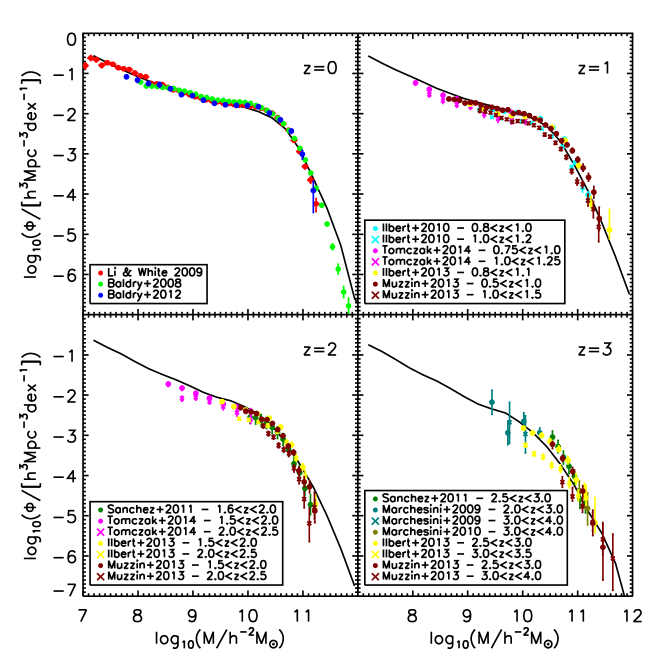
The Munich SAM, or L-Galaxies, (Springel et al., 2001; De Lucia, Kauffmann & White, 2004; Springel et al., 2005; Croton et al., 2006; De Lucia & Blaizot, 2007; Guo et al., 2011; Guo & White, 2013; Henriques et al., 2013) has been developed over the years to include most of the relevant processes that affect galaxy evolution. In this work we use its latest version, Henriques et al. (2014), and direct the reader to the appendix of that paper for a detailed description of the model. Of most relevance to this paper are the adoption of the Planck year 1 cosmology and a modified gas-to-dust relation, partly motivated by the work presented in this paper. The model parameters were constrained using the abundance and passive fractions of galaxies at $z\leq 3$; and the model has successfully reproduced key observables at these redshifts, such as the luminosity and stellar mass functions. We highlight this fact in Figure 1, which is a reproduction of the SMF at $z\in\{0,1,2,3\}$ from Henriques et al. (2014). We direct the reader to Figures 2 and A1 and the related text of that paper for a more detailed discussion, but we highlight how well the model can explain the observed evolution in the SMF at these redshifts, over the mass range constrained by observers.

2.2 Dust Extinction Model

Actively star-forming galaxies are known to be rich in dust. This can have a dramatic effect on their emitted spectrum since dust significantly absorbs optical/UV light while having a much milder effect at longer wavelengths. As a result, dust-dominated galaxies will generally have red colours even if they are strongly star-forming. For that reason, we summarise the dust model of Henriques et al. (2014) here: a fuller description can be found in Section 1.14 of the supplementary material in that paper.

We considering dust extinction separately for the diffuse interstellar medium (ISM) and for the molecular birth clouds (BC) within which stars form. The optical depth of dust as a function of wavelength is computed separately for each component and then combined as described below. We do not at present attempt to compute the detailed properties of the dust particles or the re-emission of the absorbed light.

2.2.1 Extinction by the ISM

The optical depth of diffuse dust in galactic disks is assumed to vary with wavelength as

$$\tau_{\lambda}^{ISM}= (1+z)^{-1}\left(\frac{A_{\lambda}}{A_{\mathrm{V}}}\right)_{Z_{\odot}}\left(\frac{Z_{\rm{gas}}}{Z_{\odot}}\right)^{s}$$

$$\times\left(\frac{\langle N_{H}\rangle}{2.1\times 10^{21}{\rm{atoms}}\,{\rm{cm}}^{-2}}\right),$$ (1)

where

$$\langle N_{H}\rangle=\frac{M_{\rm{cold}}}{1.4\,m_{p}\pi(aR_{\rm{gas,d}})^{2}}$$ (2)

is the mean column density of hydrogen. Here $R_{\rm{gas,d}}$ is the cold gas disk scale-length, $1.4$ accounts for the presence of helium and $a=1.68$ in order for $\langle N_{H}\rangle$ to represent the mass-weighted average column density of an exponential disk. Following the results in Guiderdoni (1987), the extinction curve in eq. (2.2.1) depends on the gas metallicity and is based on an interpolation between the Solar Neighbourhood and the Large and Small Magellanic Clouds: $s=1.35$ for $\lambda<2000$ Å  and $s=1.6$ for $\lambda>2000$ Å. The extinction curve for solar metallicity, $(A_{\lambda}/A_{\mathrm{V}})_{Z_{\odot}}$, is taken from Mathis (1983).

The redshift dependence in eq. (2.2.1) is significantly stronger than in previous versions of our model ($(1+z)^{-0.5}$ in Kitzbichler & White (2007) and $(1+z)^{-0.4}$ in Guo & White (2009)). The dependence implies that for the same amount of cold gas and the same metal abundance, there is less dust at high redshift. The motivation comes both from observations (Steidel et al., 2004; Quadri et al., 2008) and from the assumption that dust is produced by relatively long-lived stars. However, it may also be that this redshift dependence has to be introduced as a phenomenological compensation for the excessively early build-up of the metal content in model galaxies. In practice it has been included simply to give an approximate match to the low extinctions of high-redshift galaxies as inferred from their observed UV slopes (Bouwens et al., 2012), and to the UV luminosity function, as described below.

2.2.2 Extinction by molecular birth clouds

This second source of extinction affects only young stars that are still embedded in their molecular birth clouds, for which we assume a lifetime of 10 Myr. The relevant optical depth is taken to be

$$\tau_{\lambda}^{BC}=\tau_{\lambda}^{\mathrm{ISM}}\left(\frac{1}{\mu}-1\right)\left(\frac{\lambda}{5500\mathrm{\AA}}\right)^{-0.7},$$ (3)

where $\mu$ is given by a random Gaussian deviate with mean 0.3 and standard deviation 0.2, truncated at 0.1 and 1.

2.2.3 Overall extinction curve

In order to get the final overall extinction, every galaxy is assigned an inclination, $\theta$, given by the angle between the disk angular momentum and the $z$-direction of the simulation box, and a “slab” geometry is assumed for the dust in the diffuse ISM. For sources that are uniformly distributed within the disk then the mean absorption coefficient is

$$A_{\lambda}^{\mathrm{ISM}}=-2.5\log_{10}\left(\frac{1-\exp^{-\tau_{\lambda}^{\mathrm{ISM}}\sec{\theta}}}{\tau_{\lambda}^{\mathrm{ISM}}\sec{\theta}}\right),$$ (4)

Emission from young stars embedded within birth clouds is subject to an additional extinction of

$$A_{\lambda}^{\mathrm{BC}}=-2.5\log_{10}\left(\exp^{-\tau_{\lambda}^{\mathrm{BC}}}\right).$$ (5)

The standard L-Galaxies output does not attempt to model the attenuation of light by the intergalactic medium. However, this is done in post-processing for the lightcones published in the Millennium Run Observatory(Overzier et al., 2013). In this paper, however, we neglect intergalactic attenuation.

3 Recent Star Formation

In this section we investigate the star formation rate, and the related UV luminosity function, at redshifts $z\in\{4,5,6,7\}$.

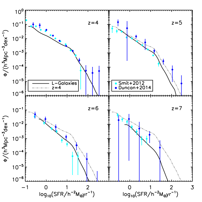
Figure 2 shows the star-formation-rate distribution function (SFR DF) as predicted by our model alongside measurements from Smit et al. (2012) (converted to our fiducial Chabrier IMF) and Duncan et al. (2014).

Comparing with the Smit et al. (2012) measurements at redshifts $z\approx 5-7$ we find generally good agreement. At these redshifts, the Duncan et al. (2014) measurements are generally higher than both the model and the Smit et al. (2012) results. This is particularly true for the most massive galaxies, though we note that the quoted observational uncertainties can be very large.

At $z\approx 4$, however, our model under-predicts the number of galaxies for $\log_{10}($SFR/$h^{-2}\mbox{M${}_{\odot}$})<1$ when compared to both sets of observations (which are consistent with one another at this redshift). The cause of the discrepancy is unclear, though may be a consequence of our model under-estimating the contribution to the SFR from merger-driven activity.

Figure 2: Predicted star formation rate distribution functions at redshift $z\approx 4$ (top left); $z\approx 5$ (top right); $z\approx 6$ (lower left) and $z\approx 7$ (lower right). In each instance we use the closest available snapshot from our L-Galaxies run of z=3.95, 5.03, 5.82 and 6.97 respectively. Solid black lines show the star formation rate distribution function predicted by our model. Our $z=4$ star formation rate distribution function is repeated at higher redshifts as a grey dot-dash line for comparison. Observations are taken from Smit et al. (2012), converted to a Chabrier IMF, and Duncan et al. (2014).

3.1 The UV Luminosity Function

We present the UV luminosity function predicted by our model in Figure 3 alongside recent observational estimations at high-redshift (Bouwens et al., 2015; Duncan et al., 2014; Finkelstein et al., 2014; Bowler et al., 2014a, b). The solid black line shows our prediction for the attenuated UV luminosity function; the attenuated UV LF at $z=4$ is also shown on subsequent plots for comparison. The dashed line shows our intrinsic UV luminosity function, with no dust model being applied.

Figure 3: Predicted rest–frame (1500 Å) UV luminosity functions at redshift $z\approx 4$ (top left); $z\approx 5$ (top right); $z\approx 6$ (lower left) and $z\approx 7$ (lower right). In each instance we use the closest snapshot available to use from our L-Galaxies run of z=3.95, 5.03, 5.82 and 6.97 respectively. Solid black lines shows the L-Galaxies prediction for the attenuated UV luminosity function using the dust extinction model outlined in §2.2.1. The dashed black line is the L-Galaxies prediction of the intrinsic UV luminosity function, with no dust model applied. Our $z=4$ attenuated UV luminosity function is repeated at higher redshifts as a grey dot-dash line for comparison. Observations are taken from Bouwens et al. (2015), Duncan et al. (2014) and Finkelstein et al. (2014), and at high mass from Bowler et al. (2014a) ($z=6$) and Bowler et al. (2014b) ($z=7$).

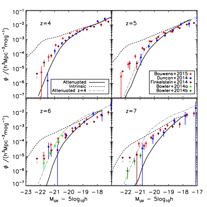
We find a good fit to the faint number counts: $M_{\mathrm{UV}}>-20$ for $z=4-6$ and $M_{\mathrm{UV}}>-19$ for $z=7$. At brighter absolute magnitudes, the model counts fall below the observed ones. Note, however, that the raw counts, before dust attenuation, lie above the observations. Given that we saw a good fit in Section 3 between predicted and observed SFRs, then this points to a difference in the dust model between the two.

To better understand this, we quantify in Figure 4 the attenuation required (as a function of the intrinsic UV absolute magnitude) to reconcile the raw L-Galaxies data with observations. We do this by comparing observed, $M_{\Phi,\mathrm{obs}}$, and intrinsic, $M_{\Phi,\mathrm{int}}$, absolute magnitudes below which we achieve a particular cumulative number density, $\Phi$ of galaxies:

$$\Phi=\int_{-\infty}^{M_{\Phi}}\phi\,\mathrm{d}M,$$ (6)

where $\phi$ is the usual differential number density of galaxies. The attenuation is then $A_{\mathrm{UV}}=M_{\Phi,\mathrm{obs}}-M_{\Phi,\mathrm{int}}$.

Figure 4: This figure shows the amount of dust attenuation required to move our intrinsic UV luminosity function (the dashed, black lines in Figure 3) to match different observational data sets (Bouwens et al., 2015; Duncan et al., 2014; Finkelstein et al., 2014), as a function of unattenuated absolute UV magnitude. The solid, black line shows the attenuation built into the L-Galaxies model as described in Section 2.2.

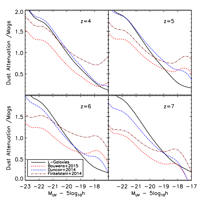
The dust attenuation required to match the observation (as a function of the intrinsic absolute magnitude) is shown in Figure 4. The black, solid line shows the attenuation currently implemented in L-galaxies, as described in Section 2.2.

As expected, the built-in attenuation matches that from the Duncan et al. (2014) data fairly well. The other data sets show a shallower slope: the attenuation is reasonable, perhaps even under-estimated in the faintest galaxies, but is strongly over-estimated in the brightest galaxies and increasingly so at high redshift.

It is important to stress that while we are presenting the results for all the objects within our simulation, observational samples (such as those employed by Bouwens et al., 2015; Duncan et al., 2014; Finkelstein et al., 2014), are biased and may not truly capture the full galaxy population at these redshifts. Indeed, a defining characteristic of the Lyman break technique, which is regularly used to identify galaxies in the high redshift universe, is that it preferentially selects blue rest-frame UV bright sources, i.e star forming galaxies with low UV dust attenuation $(\rm{A_{UV}}<2$). Very dusty galaxies, or those with little to no star formation would then be missed in typical Lyman break galaxy searches (e.g. HFLS3, a very dusty intensely star forming galaxy at $z\approx 6.3$ Riechers et al., 2013). The degree to which this is a concern at high-redshift is difficult to assess, largely due to the lack of sensitive far-IR and sub-mm imaging which is critical to identify heavily obscured systems.

Given the current observational uncertainties, we conclude that the simple, empirical dust extinction model currently built into L-galaxies does a reasonable job, although it could be refined to match particular data sets if required. In the future, we intend to implement a more physically-motivated dust model: we note that the current model has prompt recycling, and this could be an issue at these early times when the age of the Universe is just 1.5 Gyr at $z=4$ and less than 1 Gyr for $z>6$. A delayed chemical enrichment model has been implemented in L-Galaxies by Yates et al. (2013) and we intend to incorporate that into the Henriques et al. (2014) model in future work.

4 Galaxy Stellar Mass Function

We present the Galaxy Stellar Mass Function (GSMF) at $z\in\{4,5,6,7\}$ predicted by our model in Figure 5 alongside recent observational estimates at high-redshift from González et al. (2011) and Duncan et al. (2014).

Figure 5: Predicted stellar mass functions at redshift $z\approx 4$ (top left); $z\approx 5$ (top right); $z\approx 6$ (lower left) and $z\approx 7$ (lower right). In each instance we use the closest snapshot available to use from our L-Galaxies run of z=3.95, 5.03, 5.82 and 6.97 respectively. Solid black lines show the stellar mass functions predicted by our model. To indicate the possible effect of uncertainties in the observational stellar mass determinations, we also show as a red dot-dash line the stellar mass function convolved with a gaussian of standard deviation 0.3 dex. Our $z=4$ stellar mass function is repeated at higher redshifts as a grey dot-dash line for comparison. Observations are taken from González et al. (2011), converted to a Chabrier IMF, and Duncan et al. (2014).

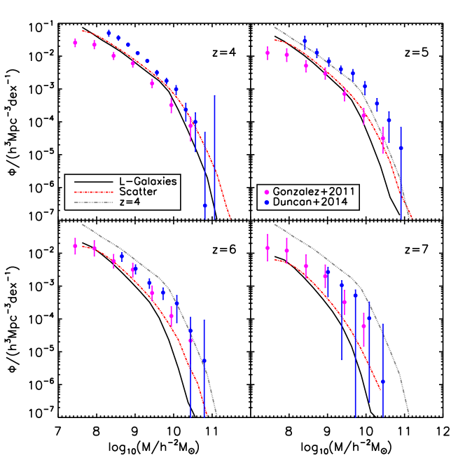
It is important to first note that the observationally-derived mass functions presented in Figure 5 are inconsistent with each other at $z\sim 4-5$. One possible source (see Duncan et al. (2014) for a wider discussion) of this discrepancy is the effect of nebular emission which was included in Duncan et al. (2014) but not in González et al. (2011). Galaxies in the high-redshift Universe are expected (Wilkins et al., 2013) and inferred (e.g. Smit et al., 2014) to exhibit strong nebular emission which can strongly affect the measured stellar mass-to-light ratios and thus masses (Wilkins et al., 2013). The accuracy/precision of stellar mass estimates are also affected by the lower sensitivity and angular resolution of the Spitzer/IRAC imaging.

Given the above observational uncertainties, it is gratifying that the model predictions split the two observational measurements at $z=4$. There is a hint that the change in slope at the “knee” of the mass-function ($M_{\mathrm{knee}}\approx 3\times 10^{9}h^{-2}$ M_⊙) may be sharper in the model than the observations, but the observational error bars are growing at this point and so it is hard to draw firm conclusions. As we move to higher redshifts, however, the model predictions and the observations gradually diverge as follows: (i) the normalisation at $M_{\mathrm{knee}}$ declines more rapidly with increasing redshift in the models than in the observations; (ii) the slope of the mass function above the knee is steeper in the models than in the observations.

Figure 6: Predicted specific star formation rates ($sSFR=SFR/M$) at redshift $z\approx 4$ (top left); $z\approx 5$ (top right); $z\approx 6$ (lower left) and $z\approx 7$ (lower right). In each instance we use the closest snapshot available to use from our L-Galaxies run of z=3.95, 5.03, 5.82 and 6.97 respectively. The histogram density plot represents the L-Galaxies galaxy population, with white representing the most dense, and blue representing the least. The solid line shows the L-Galaxies median values, and the dashed lines show the 0.16 and 0.84 percentiles. The observations are taken from Salmon et al. (2015), the points denotes the median while the error bars reflect the scatter in the observed values (not the uncertainty on the median).

The exact cause of these discrepancies is difficult to assess. One possibility is that it reflects a deficiency in the model; on the other hand it may reflect a systematic bias in the observations. This has been discussed at low redshift ($z=0-3$) in Appendix C of Henriques et al. (2013). It seems probable that the uncertainties on the individual stellar masses could have been underestimated, and that can strongly boost the inferred number of galaxies in regions where where the mass function is particularly steep. As an example of the possible magnitude of this effect, we show in Figure 5 the result of convolving with a gaussian of standard deviation 0.3 dex, similar to that required at low redshift. This largely reconciles the observed and predicted slopes of the mass function, but the normalisation remains too low at $z=7$. Understanding the source of this discrepancy is a focus of an additional work in progress (Wilkins et al. in-prep).

Recent hydrodynamic simulations, particularly Illustris (Vogelsberger et al., 2014) and Eagle (Schaye et al., 2015), have begun making predictions of observables at high redshift (Genel et al., 2014; Furlong et al., 2014). Like L-Galaxies, both Illustris and Eagle make predictions at high redshift by only using observational constraints at lower redshift. Both simulations are similar to ours in the prediction of the GSMF at $z=6-7$ in that we all under predict the abundance of high mass galaxies ($>10^{9}\mbox{M${}_{\odot}$}$) at these redshifts, although Eagle better match the observations at $z=5$ across the entire mass range. Whilst both L-Galaxies and Eagle match a similar shape to the observations, particularly finding good agreement with the slope and abundance for low mass galaxies, Illustris predicts a slope that steepens with increasing redshift faster than what is observed, and over predicts the abundance of low mass galaxies at all redshifts.

5 Specific Star Formation Rate

Figure 7: Plot to show the evolution of the stellar mass (top left); star formation rate (top right); UV luminosity function (lower left); and specific star formation rate (lower right) in the redshift range $z=4-7$. In each instance we use the closest snapshot available to use from our L-Galaxies run of z=3.95, 5.03, 5.82 and 6.97 respectively.

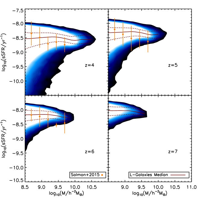
The specific star formation rate (sSFR) is a measure of how quickly a galaxy is forming its stars. We present the sSFRs at $z\in\{4,5,6,7\}$ of our galaxy population predicted by our model in Figure 6 alongside recent observational measurements from Salmon et al. (2015). We represent the sSFR of individual galaxies by a 2D histogram; the solid line shows the median value predicted by our model, averaged over bins of 100 or more galaxies.

The observations are consistent with our model, particularly for galaxies of mass $M\approx 10^{9}$ M_⊙, across all redshifts. However the observations show a decline in the sSFR with increasing galactic stellar mass and we do not identify the same trend. Instead, all galaxies in our model have roughly the same level of activity, regardless of galactic stellar mass. This discrepancy is not surprising: given that the models match the observed SFR but under-predict the stellar masses of the largest galaxies, then we would expect this result.

The question remains as to whether the observations or the model is at fault, or a combination of both. We could boost AGN feedback in the most massive galaxies in the model, but this would then reduce the bright end of the UV LF. Alternatively, as hinted in the previous section, the inferred masses of the highest-mass galaxies may have been boosted by observational scatter. At lower masses, there will be an observational bias towards the brightest galaxies, and so the median sSFR may be over-estimated.

6 Evolution

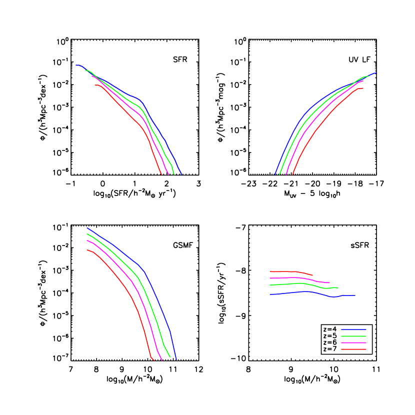
To make it easier to see how the properties of our model galaxies change with time, we extract the model predictions from each of the four redshifts shown in Figures 2, 3, 5 & 6 and display them in single panels in Figure 7.

Concentrating first on the SFR (upper-left panel), we see the the knee of the distribution remains relatively unchanged, at about $20h^{-2}$M_⊙ yr^-1 over this period. However, the normalisation of the relation grows and the slope decreases, such that the number comoving number density of galaxies with star-formation rates of $0.3h^{-2}$M_⊙ yr^-1 is approxiately constant, while that of higher star-formation rates in excess of $100h^{-2}$M_⊙ yr^-1 grows by several orders of magnitude. As might be expected, a similar, but less pronounced, trend is seen in the UV LF, although the knee of the distribution is harder to discern.

In constrast to the SFR DF, the galactic SM DF shows only a slight reduction in slope from $z=7$ to $z=4$. Consequently, the comoving number density of low-mass galaxies increases by about 1 dex over this time. This is reflected in the specfic star-formation rate, which reduces by a factor of about 0.5 dex in the same period (as the sSFR is approximately independent of mass, this conclusion holds for individual galaxis, not just the population).

7 Conclusions

We have presented the latest high-redshift observational predictions of the star-formation-rate distribution function (SFR DF); UV luminosity function (UV LF); galactic stellar mass function (GSMF) and specific star-formation rates (sSFRs) of galaxies from the latest version of the L-Galaxies semi-analytic model (Henriques et al., 2014). Our conclusions are as follows:

1. We find a good fit to both the shape and normalization of the observed SFR DF at $z=4-7$ (Figure 2), apart from a slight under-prediction at the low SFR end at $z=4$, possibly caused by a lack of SFR contribution from merger-driven activity in our model.

2. We find a good fit to the faint number counts for the observed UV LF (Figure 3). At brighter magnitudes, our predictions lie below the observations, increasingly so at higher redshifts.

3. At all redshifts and magnitudes, the raw (unattenuated) number counts for the UV LF lie above the observations, and so we interpret our under-prediction as an over-estimate of the amount of dust in the model for the brightest galaxies, especially at high-redshift (Figure 4).

4. While the shape of our SMF matches that of the observations, we lie between the observations at $z=4-5$ and under-predict at $z=6-7$ (Figure 5). We note, however, that both sets of observations are inconsistent with one another, and have, at times, large errors attached to them.

5. The sSFRs of our model galaxies (Figure 6) show the observed trend of increasing normalisation with redshift, but do not reproduce the observed mass dependence, indicating instead that galaxies of all masses the same level of activity. It is unclear as to whether this is caused by observational bias, or by an under-estimate of AGN feedback in the model.

In summary, the L-Galaxies model has mixed success in reproducing observations at high redshift. It provides a reasonable match to both the SFR DF and the low-mass end of the SMF, but fails to show the observed mass-dependence of the sSFR. The predicted UV LF is highly-dependent upon an ad-hoc scaling with redshift of the dust model.

In Yates et al. (2013) we added a detailed model of the chemical enrichment in L-Galaxies by adding a delayed enrichment from stellar winds and supernovae, as well as metallicity-dependent yields and the tracking of eleven heavy elements (including O, Mg and Fe). This shows promising results in reproducing the mass-metallicity relation at $z=0$, although the chemical enrichment at high-redshift remains untested and is something we will look at in the future. That then will provide a more realistic prediction of the metallicity of galaxies at early times. In future work, we will also add a physically-motivated model for dust growth and destruction, and consider the effect of extinction from the inter-galactic medium.

References

- Baldry et al. (2012) Baldry I. K. et al., 2012, MNRAS, 421, 621
- Baldry, Glazebrook & Driver (2008) Baldry I. K., Glazebrook K., Driver S. P., 2008, MNRAS, 388, 945
- Bouwens et al. (2009) Bouwens R. J. et al., 2009, ApJ, 705, 936
- Bouwens et al. (2008) Bouwens R. J., Illingworth G. D., Franx M., Ford H., 2008, ApJ, 686, 230
- Bouwens et al. (2010a) Bouwens R. J. et al., 2010a, ApJ, 725, 1587
- Bouwens et al. (2012) Bouwens R. J. et al., 2012, ApJ, 754, 83
- Bouwens et al. (2011) Bouwens R. J. et al., 2011, ApJ, 737, 90
- Bouwens et al. (2014) Bouwens R. J. et al., 2014, ApJ, 793, 115
- Bouwens et al. (2010b) Bouwens R. J. et al., 2010b, ApJ, 709, L133
- Bouwens et al. (2015) Bouwens R. J. et al., 2015, ApJ, 803, 34
- Bowler et al. (2014a) Bowler R. A. A. et al., 2014a, ArXiv e-prints
- Bowler et al. (2014b) Bowler R. A. A. et al., 2014b, MNRAS, 440, 2810
- Bunker et al. (2010) Bunker A. J. et al., 2010, MNRAS, 409, 855
- Castellano et al. (2012) Castellano M. et al., 2012, A&A, 540, A39
- Chabrier (2003) Chabrier G., 2003, PASP, 115, 763
- Croton et al. (2006) Croton D. J. et al., 2006, MNRAS, 365, 11
- De Lucia & Blaizot (2007) De Lucia G., Blaizot J., 2007, MNRAS, 375, 2
- De Lucia, Kauffmann & White (2004) De Lucia G., Kauffmann G., White S. D. M., 2004, MNRAS, 349, 1101
- Domínguez Sánchez et al. (2011) Domínguez Sánchez H. et al., 2011, MNRAS, 417, 900
- Duncan et al. (2014) Duncan K. et al., 2014, MNRAS, 444, 2960
- Dunlop et al. (2010) Dunlop J. S. et al., 2010, MNRAS, 408, 2022
- Dunlop et al. (2012) Dunlop J. S., McLure R. J., Robertson B. E., Ellis R. S., Stark D. P., Cirasuolo M., de Ravel L., 2012, MNRAS, 420, 901
- Ellis et al. (2013) Ellis R. S. et al., 2013, ApJ, 763, L7
- Finkelstein et al. (2010) Finkelstein S. L., Papovich C., Giavalisco M., Reddy N. A., Ferguson H. C., Koekemoer A. M., Dickinson M., 2010, ApJ, 719, 1250
- Finkelstein et al. (2012a) Finkelstein S. L. et al., 2012a, ApJ, 758, 93
- Finkelstein et al. (2012b) Finkelstein S. L. et al., 2012b, ApJ, 756, 164
- Finkelstein et al. (2014) Finkelstein S. L. et al., 2014, ArXiv e-prints
- Furlong et al. (2014) Furlong M. et al., 2014, ArXiv e-prints
- Genel et al. (2014) Genel S. et al., 2014, MNRAS, 445, 175
- González et al. (2011) González V., Labbé I., Bouwens R. J., Illingworth G., Franx M., Kriek M., 2011, ApJ, 735, L34
- Guiderdoni (1987) Guiderdoni B., Rocca-Volmerange B., 1987, A&A, 186, 1
- Guo et al. (2011) Guo Q., White S., Boylan-kolchin M., Lucia G. D., Lemson G., Li C., Springel V., Weinmann S., MNRAS, 428, 1351
- Guo & White (2009) Guo Q., White S. D. M., 2009, MNRAS, 396, 39
- Guo & White (2013) Guo Q., White S. D. M., 2013, MNRAS, 428, 1351
- Henriques et al. (2014) Henriques B., White S., Thomas P., Angulo R., Guo Q., Lemson G., Springel V., Overzier R., 2014, ArXiv e-prints
- Henriques et al. (2013) Henriques B. M. B., White S. D. M., Thomas P. A., Angulo R. E., Guo Q., Lemson G., Springel V., 2013, MNRAS, 431, 3373
- Ilbert et al. (2013) Ilbert O. et al., 2013, AAP, 556, A55
- Ilbert et al. (2010) Ilbert O. et al., 2010, ApJ, 709, 644
- Kitzbichler & White (2007) Kitzbichler M. G., White S. D. M., 2007, MNRAS, 376, 2
- Labbé et al. (2010) Labbé I. et al., 2010, ApJ, 708, L26
- Li & White (2009) Li C., White S. D. M., 2009, MNRAS, 398, 2177
- Lorenzoni et al. (2013) Lorenzoni S., Bunker A. J., Wilkins S. M., Caruana J., Stanway E. R., Jarvis M. J., 2013, MNRAS, 429, 150
- Lorenzoni et al. (2011) Lorenzoni S., Bunker A. J., Wilkins S. M., Stanway E. R., Jarvis M. J., Caruana J., 2011, MNRAS, 414, 1455
- Marchesini et al. (2009) Marchesini D., van Dokkum P. G., Förster Schreiber N. M., Franx M., Labbé I., Wuyts S., 2009, ApJ, 701, 1765
- Marchesini et al. (2010) Marchesini D. et al., 2010, ApJ, 725, 1277
- Mathis (1983) Mathis J., 1983, ApJ, 267, 119
- McLure et al. (2013) McLure R. J. et al., 2013, MNRAS, 432, 2696
- McLure et al. (2010) McLure R. J., Dunlop J. S., Cirasuolo M., Koekemoer a. M., Sabbi E., Stark D. P., Targett T. a., Ellis R. S., 2010, MNRAS, 403, 960
- McLure et al. (2011) McLure R. J. et al., 2011, MNRAS, 418, 2074
- Meurer, Heckman & Calzetti (1999) Meurer G. R., Heckman T. M., Calzetti D., 1999, ApJ, 521, 64
- Muzzin et al. (2013) Muzzin A. et al., 2013, ApJ, 777, 18
- Oesch et al. (2010) Oesch P. a. et al., 2010, ApJ, 709, L16
- Oesch et al. (2012) Oesch P. A. et al., 2012, ApJ, 745, 110
- Oesch et al. (2009) Oesch P. A. et al., 2009, ApJ, 690, 1350
- Ouchi et al. (2009) Ouchi M. et al., 2009, ApJ, 706, 1136
- Overzier et al. (2013) Overzier R., Lemson G., Angulo R. E., Bertin E., Blaizot J., Henriques B. M. B., Marleau G.-D., White S. D. M., 2013, MNRAS, 428, 778
- Planck Collaboration et al. (2014) Planck Collaboration et al., 2014, A&A, 571, A1
- Quadri et al. (2008) Quadri R. F., Williams R. J., Lee K.-S., Franx M., van Dokkum P., Brammer G. B., 2008, ApJ, 685, L1
- Riechers et al. (2013) Riechers D. a. et al., 2013, Nature, 496, 329
- Robertson et al. (2010) Robertson B. E., Ellis R. S., Dunlop J. S., McLure R. J., Stark D. P., 2010, Nature, 468, 49
- Rogers, McLure & Dunlop (2013) Rogers A. B., McLure R. J., Dunlop J. S., 2013, MNRAS, 429, 2456
- Salmon et al. (2015) Salmon B. et al., 2015, ApJ, 799, 183
- Schaye et al. (2015) Schaye J. et al., 2015, MNRAS, 446, 521
- Smit et al. (2012) Smit R., Bouwens R. J., Franx M., Illingworth G. D., Labbé I., Oesch P. a., van Dokkum P. G., 2012, ApJ, 756, 14
- Smit et al. (2014) Smit R. et al., 2014, ApJ, 784, 58
- Springel et al. (2001) Springel V., White P. S. D. M., Tormen G., Kauffmann G., 2001, MNRAS, 328, 726
- Springel et al. (2005) Springel V. et al., 2005, Nature, 435, 629
- Stanway, McMahon & Bunker (2005) Stanway E. R., McMahon R. G., Bunker A. J., 2005, MNRAS, 359, 1184
- Stark et al. (2009) Stark D. P., Ellis R. S., Bunker A., Bundy K., Targett T., Benson A., Lacy M., 2009, ApJ, 697, 1493
- Steidel et al. (2004) Steidel C. C., Shapley A. E., Pettini M., Adelberger K. L., Erb D. K., Reddy N. A., Hunt M. P., 2004, ApJ, 604, 534
- Tomczak et al. (2014) Tomczak A. R. et al., 2014, ApJ, 783, 85
- Vogelsberger et al. (2014) Vogelsberger M. et al., 2014, Nature, 509, 177
- Wilkins et al. (2013) Wilkins S. M., Bunker A., Coulton W., Croft R., Matteo T. D., Khandai N., Feng Y., 2013, MNRAS, 430, 2885
- Wilkins et al. (2010) Wilkins S. M., Bunker A. J., Ellis R. S., Stark D., Stanway E. R., Chiu K., Lorenzoni S., Jarvis M. J., 2010, MNRAS, 403, 938
- Wilkins et al. (2011a) Wilkins S. M., Bunker A. J., Lorenzoni S., Caruana J., 2011a, MNRAS, 411, 23
- Wilkins et al. (2011b) Wilkins S. M., Bunker A. J., Stanway E., Lorenzoni S., Caruana J., 2011b, MNRAS, 417, 717
- Wilkins et al. (2012) Wilkins S. M., Gonzalez-Perez V., Lacey C. G., Baugh C. M., 2012, MNRAS, 424, 1522
- Yan et al. (2012) Yan H. et al., 2012, ApJ, 761, 177
- Yates et al. (2013) Yates R. M., Henriques B., Thomas P. A., Kauffmann G., Johansson J., White S. D. M., 2013, MNRAS, 435, 3500