Group structures and representations of graph states

Abstract

A special configuration of graph state stabilizers, which contains only Pauli $\sigma_{X}$ operators, is studied. The vertex sets $\xi$ associated with such configurations are defined as what we call X-chains of graph states. The X-chains of a general graph state can be determined efficiently. They form a group structure such that one can obtain the explicit representation of graph states in the X-basis via the so-called X-chain factorization diagram. We show that graph states with different X-chain groups can have different probability distributions of X-measurement outcomes, which allows one to distinguish certain graph states with X-measurements. We provide an approach to find the Schmidt decomposition of graph states in the X-basis. The existence of X-chains in a subsystem facilitates error correction in the entanglement localization of graph states. In all of these applications, the difficulty of the task decreases with increasing number of X-chains. Furthermore, we show that the overlap of two graph states can be efficiently determined via X-chains, while its computational complexity with other known methods increases exponentially.

I Introduction

Graph states BriegelRaussendorf2001-FirstGrSt ; RaussendorfBriegel2001-05 ; RaussendorfBriegel2002-10 ; RaussendorfBrowneBriegel2003-08 ; RaussendorfPHDThesis2003 ; HeinEisertBriegel2004-06 ; GraphStateReviews2006 represent specific multipartite entangled quantum systems. They are an important resource for measurement-based quantum computation: there, the multipartite entanglement of cluster states (a special class of graph states) is consumed by local measurements on subsystems. Depending on the measurement outcomes, local unitary transformations of the remaining systems are performed. In this way, certain quantum operations can be implemented.

Graph states can be represented in the stabilizer formalism as eigenstates of certain tensor products of Pauli $\sigma_{X}$- and $\sigma_{Z}$-operators (the graph state stabilizers). The explicit structure of the stabilizer operators depends on the structure of the underlying graph. The stabilizers form a group (under multiplication), which is generated from $n$ generators, where $n$ is the number of vertices of the graph.

In this paper, we will discuss what we call X-chains. X-chains are subsets of vertices of a given graph which correspond to graph state stabilizers that consist only of Pauli $\sigma_{X}$-operators. We will show that these X-chains form a group. Not every graph contains an X-chain. However, it will be shown that if a graph does contain X-chains, this fact can be used as an efficient tool to determine essential properties of the corresponding graph state, such as its overlap with other graph states, its entanglement characteristics, and the existence of error correcting code words in subsystems of graph states. Note that the overlap of two graph states cannot be determined efficiently to date. The X-chains provide an efficient method to solve this problem.

While graph states are usually given in the Z-basis, the concepts and methods developed in this paper show that it is often favorable to represent graph states in the X-basis, in particular when one wants to study overlaps of graph states or determine their entanglement properties. The reason for this fact is that for all graph states originating from the same number of vertices, the probability distribution of outcomes of local Z-measurements is uniform, while it is nonuniform for outcomes of local X-measurements. Different X-measurement outcomes of two graph states reflect their difference in the X-chain groups, as the existence of an X-chain in a graph state implies vanishing probability of certain X-measurement outcomes. Conversely, X-chain groups of graph states determine their representation in the X-basis.

In the present paper we will focus on introducing the concept of X-chains, illustrating it with examples, and presenting some applications. The X-chain group of a given graph state can be efficiently determined, the search of X-chains in a given graph state will be studied in detail elsewhere WuKampermannBruss2015-XChainAlgo and a MATHEMATICA package is available in the Supplemental Material XchainMpackage_Wu .

This paper is organized as follows. In section I.1, we review the essential concepts of graph theory and graph states. In section II, we review the representation of graph states in the Z-basis and point out its disadvantage in distinguishing graph states. Then we introduce X-chains and study their properties in section III. The representation of graph states in the X-basis is derived via the so-called X-chain factorization in section IV, where we show how X-chain groups feature the X-measurement outcomes on graph states. In section V, we discuss several applications of X-chains, namely the calculation of the overlap of two graphs states (section V.1), the Schmidt decomposition of graph states in the X-basis (section V.2) and the entanglement localization PoppVMCirac2005-LocalizableEnt of graph states against errors (section V.2.1). The proofs are presented in Appendix A. A list of notations and symbols is given in Appendix B.

I.1 Basic concepts

Here we review the concepts of graphs Diestel_GraphTheory and graph states HeinEisertBriegel2004-06 ; GraphStateReviews2006 , and introduce the notation used in the main text.

Graph theory Diestel_GraphTheory :

$G$ V_G E_G N_v G[ξ] A graph $G=(V,E)$ consists of $n$ vertices $V$ and $l$ edges $E$. The vertices, denoted by $V_{G}=\left\{v_{1},...,v_{n}\right\}$, are depicted as dots and represent locations, particles etc. The edges, denoted by $E_{G}=\left\{e_{1},...,e_{l}\right\}$, describe a relation network between vertices. A symmetric relation between two vertices $v_{1}$ and $v_{2}$, e.g. a two-way bridge between two islands, can be represented by the vertex set $e=\{v_{1},v_{2}\}$, which is called undirected edge. Let $\xi_{a},\xi_{b}\subseteq V_{G}$ be two subsets of $V_{G}$, then the edges between $\xi_{a}$ and $\xi_{b}$ are the edges $e=\{v_{a},v_{b}\}$, which have one vertex $v_{a}\in\xi_{a}$ and another vertex $v_{b}\in\xi_{b}$. The set of these edges is denoted by $E_{G}(\xi_{a}:\xi_{b})$. A vertex $v_{1}$ is a neighbor of $v_{2}$, if they are connected by an edge. The set of all neighbors of $v$, called the neighborhood of $v$, is denoted as $N_{v}$. In Table 1 we list two of the relevant types of graphs, which will be considered in the main text.

Name of graph	Graph	Definition
Star graph $S_{n}$		Graphs, for which the center vertex has $n-1$ neighbors and all the others have the center vertex as their only neighbor.
Cycle graph $C_{n}$		Graphs, for which every vertex has degree $2$. They are closed paths.

Table 1: The graphs considered in this paper.

A graph $F$ is a subgraph of $G$, if its vertices and edges are subsets of the vertex set and the edge set of $G$, respectively, i.e., $V_{F}\subseteq V_{G}$ and $E_{F}\subseteq E_{G}$. A subgraph induced by a vertex set $\xi\subseteq V_{G}$ is defined as the graph

$$G[\xi]:=(\xi,E_{G}(\xi:\xi)),$$ (1)

which has the edge set $E_{G}(\xi:\xi)$ consisting of edges between vertices inside the set $\xi$.

Binary notation:

—i_α^(ι)⟩ In this paper, we use binary numbers to denote a subset of vertices of graphs. Let $G$ be a graph with vertices $V_{G}=\left\{1,...,n\right\}$ and $\xi\subseteq V_{G}$ be a vertex subset. We denote the binary number of $\xi$ as

$$i^{(\xi)}:=i_{1}\cdots i_{n},$$ (2)

with

$$i_{j}=\left\{\begin{array}[c]{cc}0&,j\not\in\xi\\ 1&,j\in\xi\end{array}\right..$$

For example, in a 4-vertex graph, $0110=i^{\left\{2,3\right\}}$. The tensor product of Pauli-operators $\sigma_{\alpha}$ with $\alpha\in\{x,y,z\}$ is denoted as

$$\sigma_{\alpha}^{(\xi)}:=\sigma_{\alpha}^{i_{1}\left(\xi\right)}\otimes\cdots\otimes\sigma_{\alpha}^{i_{n}\left(\xi\right)},$$ (3)

with $\sigma_{\alpha}^{0}=\mathbbm{1},\sigma_{\alpha}^{1}=\sigma_{\alpha}$. For example, for $n=4$, $\sigma_{\alpha}^{\left\{2,3\right\}}:=\mathbbm{1}\otimes\sigma_{\alpha}\otimes\sigma_{\alpha}\otimes\mathbbm{1}$.

II Representation of graph states

g_i s_G^(ξ) S_G P(V_G) We review the representation of graph states HeinEisertBriegel2004-06 ; GraphStateReviews2006 . A given graph with $n$ vertices has a corresponding quantum state by associating each vertex $v_{i}$ with a graph state stabilizer generator $g_{i}$,

$$g_{i}=\sigma_{X}^{(i)}\sigma_{Z}^{(N_{i})}.$$ (4)

Here, $N_{i}$ is the neighborhood of the vertex $v_{i}$. A graph state $|G\rangle$ is the $n$-qubit state stabilized by all $g_{i}$, i.e.,

$$g_{i}|G\rangle=|G\rangle,\text{for all }i=1,...,n.$$ (5)

The $n$ graph state stabilizer generators, $g_{i}$, generate the whole stabilizer group $\left(\mathcal{S}_{G},\cdot\right)$ of $|G\rangle$ with multiplication as its group operation. The group $\mathcal{S}_{G}$ is Abelian and contains $2^{n}$ elements. These $2^{n}$ stabilizers uniquely represent a graph state on $n$ vertices. Let us define the“induced stabilizer”, which is uniquely associated with a given vertex subset.

Definition 1 (Induced stabilizer).

s_G^(ξ) Let $G$ be a graph on vertices $V_{G}=\left\{v_{1},v_{2},\cdots,v_{n}\right\}$. Let $\xi$ be a subset of $V_{G}$. We call the product of all $g_{i}$ with $i\in\xi$, i.e.

$$s_{G}^{(\xi)}:=\prod_{i\in\xi}g_{i},$$ (6)

the $\xi$-induced stabilizer of the graph state $|G\rangle$. Here, $g_{i}$ is the graph state stabilizer generator of $|G\rangle$ associated with the $i$-th vertex.

Since this $\xi$-induction map is bijective, it maps the group $\left(\mathcal{P}\left(V_{G}\right),\Delta\right)$ into the stabilizer group $\left(\mathcal{S}_{G},\cdot\right)$, where $\mathcal{P}\left(V_{G}\right):=\left\{\xi\subseteq V_{G}\right\}$ is the power set (the set of all subsets) of $V_{G}$ and $\Delta$ is the symmetric difference operation acting on two sets as $\xi_{1}\Delta\xi_{2}=(\xi_{1}\setminus\xi_{2})\cup(\xi_{2}\setminus\xi_{1})$.

Proposition 2 (Isomorphism of $\xi$-induction).

Let $\left(\mathcal{S}_{G},\cdot\right)$ be the stabilizer group of a graph state $|G\rangle$ and $\mathcal{P}(V_{G})$ be the power set of the vertex set of $G$. The vertex-induction operation $s_{G}^{(\xi)}$ is a group isomorphism between $(\mathcal{P}(V_{G}),\Delta)$ and $(\mathcal{S}_{G},\cdot)$, i.e.

$$(\mathcal{P}(V_{G}),\Delta)\overset{s_{G}^{(\xi)}}{\sim}\left(\mathcal{S}_{G},\cdot\right),$$ (7)

where $\Delta$ is the symmetric difference operation.

Proof.

See Appendix A. ∎

The summation operation maps the stabilizer group $\mathcal{S}_{G}$ to its stabilized space, i.e. the density matrix of the graph state $|G\rangle$ GraphStateReviews2006 ,

$$\mathcal{S}_{G}\overset{\Sigma}{\longrightarrow}|G\rangle\langle G|=\frac{1}{2^{n}}\sum_{s\in S_{G}}s.$$ (8)

Hence there also exists an operation mapping the group $\mathcal{P}(V_{G})$ to graph states

$$\mathcal{P}(V_{G})\overset{\Sigma\circ s_{G}^{(\xi)}}{\longrightarrow}|G\rangle\langle G|=\frac{1}{2^{n}}\sum_{\xi\subseteq V_{G}}s_{G}^{(\xi)}=\prod_{i=1}^{n}\frac{1+g_{i}}{2}.$$ (9)

This is a well-known representation of graph states GraphStateReviews2006 . The representation of a graph state in the computational Z-basis $|i_{Z}\rangle$ VandenNest2005-PhDthesis is given by

$$\mathcal{P}(V_{G})\overset{\Sigma\circ s_{G}^{(\xi)}\text{ in }|i_{Z}\rangle}{\longrightarrow}|G\rangle=\frac{1}{2^{n/2}}\sum_{i\in\{0,1\}^{\otimes n}}\left(-1\right)^{\left\langle i,i\right\rangle_{A_{G}}}|i_{Z}\rangle.$$ (10)

Here $\sigma_{z}^{\otimes n}|i_{Z}\rangle=\left(-1\right)^{\left|i\right|}|i_{Z}\rangle$, where $\left|i\right|$ is the Hamming weight of $i$. $A_{G}$ $A_{G}$ is the adjacency matrix of the graph $G$, and $\braket{i,i}_{A_{G}}=(i_{1},...,i_{n})A_{G}(i_{1},...,i_{n})^{\mathrm{T}}$. For all graph states with $n$ vertices, the probability amplitudes of Z-basis states $\langle i_{Z}|G\rangle$ are homogenously distributed for all $|i_{Z}\rangle$ up to a phase $-1$, i.e. $|\braket{i_{Z}}{G}|=1/2^{n/2}$. Therefore graph states with the same vertex set all have the equivalent probability distribution of local $\sigma_{Z}$-measurement outcomes. This means that the Z-basis representation conceals the inner structure of graph states.

Different from the Z-basis, the representation of graph states in the computational X-basis $|i_{X}\rangle$ ( i.e. $\sigma_{X}^{\otimes n}|i_{X}\rangle=\left(-1\right)^{\left|i\right|}|i_{X}\rangle$) reveals the structure of graph states to a certain degree. One aim in this paper is to find an efficient algorithm, i.e. a mapping from $\mathcal{P}(V_{G})$ to $|G\rangle$, to represent graph states in the computational X-basis:

$$\mathcal{P}(V_{G})\overset{?}{\longrightarrow}|G\rangle\text{ in }|i_{X}\rangle.$$ (11)

In the rest of the paper, we denote the X-basis $|i_{X}\rangle$ as $|i\rangle$; that is, $|0\rangle=|+_{Z}\rangle=(\ket{0_{Z}}+\ket{1_{Z}})/\sqrt{2}$ and $|1\rangle=|-_{Z}\rangle=(\ket{0_{Z}}-\ket{1_{Z}})/\sqrt{2}$.

III X-chains and their properties

The commutativity of the measurement setting with graph state stabilizers determines whether one can obtain information about a graph state in the laboratory. Graph state stabilizers that commute with $\sigma_{X}$-measurements are the stabilizers consisting of solely $\sigma_{X}$ operators. They are the key ingredient in the representation of graph states in the X-basis. We will call the vertex sets $\xi$ inducing such configurations X-chains of graph states. In this section, the concept of X-chains will be introduced and their properties will be investigated.

The number of $\sigma_{Z}$-operators in the graph state stabilizer $s_{G}^{(\xi)}$ depends on the neighborhoods within the vertex set $\xi$. If a vertex $v$ has an even number of neighbors within $\xi$, then the Pauli operator $\sigma_{Z}^{(v)}$ appears an even number of times in $s_{G}^{(\xi)}$, such that the product becomes the identity. Therefore to find the X-chain configurations of graph states, one needs to study the symmetric difference of neighborhoods within the vertex set $\xi$, which we define as the correlation index of $\xi$ as follows.

Definition 3 (Correlation index).

c_ξ Let $\xi$ be a vertex subset of a graph $G$. Its correlation index is defined as the symmetric difference of neighbourhoods within $\xi$,

$$c_{\xi}:=N_{v_{1}}\Delta N_{v_{2}}\cdots\Delta N_{v_{k}},$$ (12)

where $N_{v_{i}}$ is the neighbourhood of $v_{i}$ and $\xi=\{v_{1},...,v_{k}\}$.

The name “correlation index” will become clearer in Theorem 13 and refers to the fact that for vanishing correlation index the corresponding stabilized state is factorized. (These states are called X-chain states in Def. 9.) Note that the set $c_{\xi}$ occurs as an “index” for the $\sigma_{Z}$ operator of the induced stabilizer $s_{G}^{(\xi)}$ (see Proposition 5).

Besides the correlation index, due to the anticommutativity of $\sigma_{X}$ and $\sigma_{Z}$, the graph state stabilizers also depend on the so-called stabilizer parity of $\xi$.

Definition 4 (Stabilizer parity).

π_G(ξ)Let $\xi$ be a vertex subset of a graph $G$. Its stabilizer parity in $\ket{G}$ is defined as the parity of the edge number $\left|E_{G[\xi]}\right|$ of the $\xi$-induced subgraph $G[\xi]$

$$\pi_{G}\left(\xi\right):=(-1)^{\left|E_{G[\xi]}\right|}.$$ (13)

The stabilizer parity of $\xi$, $\pi_{G}\left(\xi\right)$ is positive if the edge number $E(G[\xi])$ is even, otherwise it is negative. The explicit form of the induced stabilizers is given in the following proposition.

Proposition 5 (Form of the induced stabilizer).

Let $\xi$ be a vertex subset of a graph $G$. The $\xi$-induced stabilizer (see Def. 1) of a graph state $|G\rangle$ is given by

$$s_{G}^{(\xi)}=\pi_{G}\left(\xi\right)\sigma_{X}^{(\xi)}\sigma_{Z}^{(c_{\xi})},$$ (14)

where $c_{\xi}$ is the correlation index of $\xi$ and $\pi_{G}\left(\xi\right)$ is the stabilizer parity of $\xi$.

Proof.

See Appendix A. ∎

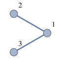
(a)

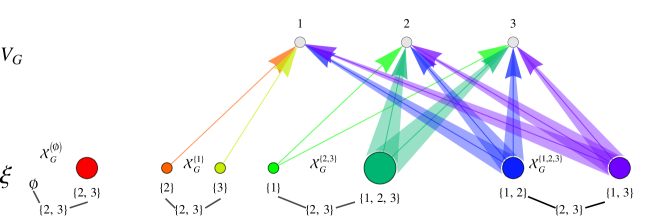
(b)

$\xi$	$\emptyset$ and $\{2,3\}$	$\{2\}$ and $\{3\}$	$\{1\}$ and $\{1,2,3\}$	$\{1,2\}$ and $\{1,3\}$
$c_{\xi}\in\mathcal{C}_{G}$	$\emptyset$	$\{1\}$	$\{2,3\}$	$\{1,2,3\}$
$|E_{G[\xi]}|$	$0$	$0$	$0$ and $2$	$1$
$\pi_{G}\left(\xi\right)$	$1$	$1$	$1$	$-1$
$s_{G}^{(\xi)}$	$\mathbbm{1}$, $\sigma_{X}^{\{2,3\}}$	$\sigma_{X}^{\{2\}}\sigma_{Z}^{\{1\}}$, $\sigma_{X}^{\{3\}}\sigma_{Z}^{\{1\}}$	$\sigma_{X}^{(1)}\sigma_{Z}^{\{2,3\}}$, $\sigma_{X}^{\{1,2,3\}}\sigma_{Z}^{\{2,3\}}$	$-\sigma_{x}^{\{1,2\}}\sigma_{Z}^{\{1,2,3\}}$, $-\sigma_{X}^{\{1,3\}}\sigma_{Z}^{\{1,2,3\}}$
$\xi\in\langle\mathcal{K}_{G}\rangle$	$\emptyset$	$\{2\}$	$\{1\}$	$\{1,2\}$
	$\Gamma_{G}=\{\{2,3\}\}$, $\mathcal{K}_{G}=\{\{1\},\{2\}\}$

(c)

Figure 1: (Color online) Correlation indices and X-resources: (a) $3$-vertex star graph. (b) The mapping from X-resources to correlation indices is illustrated in the incidence structure Rosen1999combinatorial of the graph $S_{3}$. The upper line is the correlation index, while the lower line are the vertex subsets (including the empty set). The arrows go from lower vertex subsets $\xi$ to the upper vertices corresponding to the nonzero entries of their correlation index $c_{\xi}$. For example, the vertex set $\{1,2,3\}$ points to the vertices $\{2,3\}$, indicating that the correlation index of $\{1,2,3\}$ is $c_{\{1,2,3\}}=\{2,3\}$. In particular, the vertex set $\emptyset$ and $\{2,3\}$ are X-chains (see Def. 7), since their correlation index is $\emptyset$. The resources in the sets $\mathcal{X}_{G}^{(\emptyset)}=\{\emptyset,\{2,3\}\}$, $\mathcal{X}_{G}^{\{1\}}=\{\{2\},\{3\}\}$, $\mathcal{X}_{G}^{\{2,3\}}=\{\{1\},\{1,2,3\}\}$ and $\mathcal{X}_{G}^{\{1,2,3\}}=\{\{1,2\},\{1,3\}\}$ are all “connected” by $\{2,3\}$ via the symmetric difference operation $\Delta$. (c) Grouping of vertex subsets according to the correlation index. $\Gamma_{G}$ and $\mathcal{K}_{G}$ are the X-chain group generators and correlation group generators, respectively.

Let us illustrate these concepts with an example. The star graph state $|S_{3}\rangle$ is shown in Fig. 1a. Its stabilizers can be represented in the following binary matrix:

$$\left(\begin{array}[c]{ccc|ccc}0&0&0&0&0&0\\ 1&0&0&0&1&1\\ 0&1&0&1&0&0\\ 0&0&1&1&0&0\\ 1&1&0&1&1&1\\ 1&0&1&1&1&1\\ 0&1&1&0&0&0\\ 1&1&1&0&1&1\end{array}\right),$$

in which each row represents a stabilizer. The bit strings on the left hand side of the divider are the possible vertex sets $\xi$ occurring as a superscript for the Pauli $\sigma_{X}$ operators in Eq. (14), while the right hand side is their correlation indices $c_{\xi}$ occurring as a superscript for the Pauli $\sigma_{Z}$ operators. This is the so-called binary representation of graph states Gottesman1997-phdQEC ; Gottesman1996-QECSQHB ; CalderbankRSSloane1997-QECOrthGeo . We interpret this binary representation as an incidence structure Rosen1999combinatorial in Fig. 1b, in which the vertex sets $\xi$ are depicted as the nodes in the lower row, while the upper row interprets the correlation indices $c_{\xi}$ . In the example of $|S_{3}\rangle$, one observes that the correlation indices $c_{\xi}$ do not cover all possible $3$-bit binary numbers. The vertex subsets are regrouped according to their correlation indices in Fig. 1c. The concept of regrouping is introduced via the definition of the so-called X-resources as follows.

Definition 6 (X-resources of correlation indices).

We denote the set of correlation indices of a graph $G$ as

$$\mathcal{C}_{G}:=\left\{c_{G}(\xi):\xi\subseteq V_{G}\right\}.$$

If a vertex set $\xi$ has correlation index $c$, i.e. $c_{G}(\xi)=c$, then we call $\xi$ an (X-)resource of $c$-correlation in $G$. The (X-)resource set of $c$-correlation is written as

$$\mathcal{X}_{G}^{\left(c\right)}:=\left\{\xi\subseteq V_{G}:c_{G}(\xi)=c\right\}.$$ (15)

C_GX_G^(c)

Since in the example of $\ket{S_{3}}$ the correlation index of $\{2,3\}$ is $\emptyset$, each correlation index $c\in\mathcal{C}_{S_{3}}$ has two X-resources $\xi^{(c_{1})}$ and $\xi^{(c_{2})}$ with $\xi^{(c_{1})}=\xi^{(c_{2})}\Delta\{2,3\}$. The number of X-resources of $\ket{S_{3}}$ is $2^{3}$. Therefore the graph state $|S_{3}\rangle$ generates $4$ correlation indices corresponding to $4$ binary numbers. The other $4$ correlation indices are excluded due to the existence of the non-trivial $\emptyset$-correlation resource $\{2,3\}$. This non-trivial $\emptyset$-correlation resource decreases the correlations of the graph state in the X-basis. Explicitly a non-trivial $\emptyset$-correlation resource induces a stabilizer consisting solely of $\sigma_{X}$ operators as follows.

$$s_{G}^{(\xi)}=\pi_{G}\left(\xi\right)\sigma_{X}^{(\xi)}\text{, for all }\xi\in\mathcal{X}_{G}^{\left(\emptyset\right)}.$$

We will call such vertex sets X-chains.

Definition 7 (X-chains).

Let $|G\rangle$ be a graph state. An X-resource of $\emptyset$-correlation in $G$ is called an X-chain of $G$. The set of all X-chains is denoted as $\mathcal{X}_{G}^{\left(\emptyset\right)}$. X_G^(∅)

The X-chains of a graph state $\ket{G}$ can be determined efficiently with standard linear algebra tools WuKampermannBruss2015-XChainAlgo . As examples, the X-chains of the graph states $|S_{3}\rangle$, $|S_{4}\rangle$ and $|C_{3}\rangle$ are given in Table 2. Besides, the X-chains for certain types of graph states (i.e. linear graph states $\ket{L_{n}}$, cycle graph states $\ket{C_{n}}$, complete graph states $\ket{K_{n}}$ and star graph states $\ket{S_{n}}$) are studied in WuKampermannBruss2015-XChainAlgo . A MATHEMATICA package is provided for finding X-chains in general graph states; see Supplemental Material XchainMpackage_Wu .

Graph $G$	X-chains $\braket{\Gamma_{G}}$	X-chain generators $\Gamma_{G}$
$S_{3}$		{{2,3}}
$C_{3}$		$\{\{1,2,3\}\}$
$S_{4}$		$\{\{2,3\},\{2,4\}\}$

Table 2: X-chain groups of simple graphs: The directed graphs shown under the X-chains illustrate the criterion of X-chains. Once a vertex is selected in a vertex subset, one draws arrows from it to its neighbors. A vertex subset $\xi$ is an X-chain if and only if all vertices of the graph are incident by even number of arrows. The X-chain groups $\braket{\Gamma_{G}}$ are generated by their generating sets $\Gamma_{G}$.

We point out that the X-chains form a group with the symmetric difference operation.

Lemma 8 (X-chain groups and correlation groups).

Let $|G\rangle$ be a graph state. The set of X-chains together with the symmetric difference $(\mathcal{X}_{G}^{\left(\emptyset\right)},\Delta)$, is a normal subgroup of $\left(\mathcal{P}\left(V_{G}\right),\Delta\right)$. The quotient group $(\mathcal{P}\left(V_{G}\right)/\mathcal{X}_{G}^{\left(\emptyset\right)},\Delta)$ is identical to the set of all resource sets

$$\mathcal{P}\left(V_{G}\right)/\mathcal{X}_{G}^{\left(\emptyset\right)}=\left\{\mathcal{X}_{G}^{\left(c\right)}:c\in\mathcal{C}_{G}\right\},$$ (16)

which we call call the correlation group of $\ket{G}$. Let $\Gamma_{G}$ and $\mathcal{K}_{G}$ denote the generating sets of $(\mathcal{X}_{G}^{\left(\emptyset\right)},\Delta)$ and $(\mathcal{P}(V_{G})/\mathcal{X}_{G}^{(\emptyset)},\Delta)$, respectively. The stabilizer group $\left(\mathcal{S}_{G},\cdot\right)$ is isomorphic to the direct product of the X-chain group and the correlation group,

$$\left(\mathcal{S}_{G},\cdot\right)\sim\left(\left\langle\Gamma_{G}\right\rangle,\Delta\right)\times\left(\left\langle\mathcal{K}_{G}\right\rangle,\Delta\right),$$ (17)

As a result, the graph state $|G\rangle$ is the product of the X-chain group and correlation group inducing stabilizers, i.e.

$$|G\rangle\langle G|=\prod_{\kappa\in\mathcal{K}_{G}}\frac{1+s_{G}^{(\kappa)}}{2}\prod_{\gamma\in\Gamma_{G}}\frac{1+s_{G}^{(\gamma)}}{2}.$$ (18)

⟨Γ_G⟩⟨K_G⟩⟨K⟩

Proof.

See Appendix A. ∎

Note that the brackets $\braket{\Gamma_{G}}$ and $\braket{\mathcal{K}_{G}}$ denote the group generated by $\Gamma_{G}$ and $\mathcal{K}_{G}$, respectively The correlation group represents the partition of the powerset of vertex set $\mathcal{P}(V_{G})$ regarding the correlation index of the vertex subsets $\xi\in\mathcal{P}(V_{G})$. The members in the correlation group $\xi\in\braket{\mathcal{K}_{G}}$ possess distinct correlation indices. All of the members in the $c$-correlation resource set $\xi\in\mathcal{X}^{(c)}$ are connected by X-chains. Let $\xi_{1}^{(c)}\in\mathcal{X}^{(c)}$ and $\xi_{2}^{(c)}\in\mathcal{X}^{(c)}$ be two X-resources for the same correlation index $c$. Then there must exist an X-chain $\gamma\in\Gamma_{G}$, such that

$$\xi_{2}^{(c)}=\xi_{1}^{(c)}\Delta\gamma.$$ (19)

For instance, in the example of $|S_{3}\rangle$ (Fig. 1b), the resources of correlation $i^{(c)}=111$ (i.e. $c=\left\{1,2,3\right\}$) are connected by the X-chain $\{2,3\}$, i.e. $\{1,3\}=\{1,2\}\Delta\{2,3\}$. Therefore, one can choose one member in $\mathcal{X}^{(c)}$ to represent the whole resource set $\mathcal{X}^{(c)}$. Hence, after the X-chain factorization the group $\left(\mathcal{P}\left(V_{G}\right),\Delta\right)$ for $S_{3}$ becomes $\left\langle\mathcal{K}_{G}\right\rangle=\left\{\emptyset,\left\{1\right\},\left\{2\right\},\left\{1,2\right\}\right\}$ with $\mathcal{K}_{G}=\left\{\left\{1\right\},\left\{2\right\}\right\}$

In Eq. (18), the Hilbert space $\mathbb{H}_{G}$ of the graph state $\ket{G}$ is first projected onto the subspace stabilized by the stabilizers $s_{G}^{(\gamma)}$ with $\gamma\in\Gamma_{G}$. It is the subspace, $\mathrm{span}\left(\Psi_{\emptyset}\right)$, spanned by the stabilized states $|\psi_{\emptyset}\rangle$ with

$$\Psi_{\emptyset}:=\left\{|\psi_{\emptyset}\rangle:s_{G}^{(\gamma)}|\psi_{\emptyset}\rangle=|\psi_{\emptyset}\rangle\text{, for all }\gamma\in\Gamma_{G}\right\}.$$ (20)

In this projection, $\ket{\psi_{\emptyset}}$ are all product states, since every X-chain stabilizer $s_{G}^{(\gamma)}$ commutes with the $\sigma^{\otimes n}_{X}$ operator. After the first projection, the graph state is then obtained via projecting the subspace $\mathrm{span}\left(\Psi_{\emptyset}\right)$ into the state that is stabilized by the stabilizers $s_{G}^{(\kappa)}$ induced by the correlation group; that is,

$$\mathbb{H}_{G}\overset{\Gamma_{G}}{\longrightarrow}\Psi_{\emptyset}\overset{\mathcal{K}_{G}}{\longrightarrow}|G\rangle.$$ (21)

This approach will be employed in the next section to derive the representation of graph states in the X-basis.

IV X-chain factorization of graph states

We express $|G\rangle$ in the X-basis as $|G\rangle=\sum_{i=1}^{2^{n}}\alpha_{i}|i_{X}\rangle$, with $\sum_{i}|\alpha_{i}|^{2}=1$. Since the X-chain stabilizers $s_{G}^{(\gamma)}$ stabilize $|G\rangle$, it holds that

$$\sum\alpha_{i}|i_{X}\rangle=\sum\alpha_{i}s_{G}^{(\gamma)}|i_{X}\rangle.$$ (22)

Since $s_{G}^{(\gamma)}$ solely contains $\sigma_{X}$-operators, $s_{G}^{(\gamma)}|i_{X}\rangle=\pm|i_{X}\rangle$. In order to fulfill Eq. (22), however, it follows that only the plus sign is possible, i.e.

$$s_{G}^{(\gamma)}|i_{X}\rangle=|i_{X}\rangle\text{ for all }\alpha_{i}\not=0.$$ (23)

That means that the possible X-measurement outcomes are solely those X-basis states $|i_{G}\rangle$, which are stabilized by all X-chain stabilizers $s_{G}^{(\gamma)}$. A graph state $|G\rangle$ is hence a superposition of such particular X-basis states.

For example, the star graph state $|S_{3}\rangle$ in Fig. 1 is stabilized by the X-chain stabilizer $s_{S_{3}}^{\{2,3\}}=\sigma_{X}^{\{2,3\}}$. Therefore $\ket{S_{3}}$ belongs to the space spanned by the states stabilized by $s_{S_{3}}^{\{2,3\}}$. From the table in Fig. 1, one observes that the X-basis $|i^{(c)}\rangle$, with $c\in\mathcal{C}_{S_{3}}$ (see Def. 6) corresponding to the correlation indices of $|S_{3}\rangle$, are stabilized by $s_{S_{3}}^{\{2,3\}}$, i.e. $\sigma_{X}^{(\{2,3\})}\ket{i^{(c)}}=\ket{i^{(c)}}$ for all $c\in\mathcal{C}_{S_{3}}$. That means $|S_{3}\rangle$ belongs to the subspace, $\mathrm{span}(\Psi)$, spanned by $\Psi=\left\{|i^{(c)}\rangle,c\in\mathcal{C}_{S_{3}}\right\}=\left\{|000\rangle,|100\rangle,|011\rangle,|111\rangle\right\}$. Thus $|S_{3}\rangle$ can be represented solely in $4$ X-basis states instead of $8$ $Z$-basis states.

In this section, we will derive a general mapping from the X-chain group and correlation group to graph states in the X-basis. This is the question we raised in section II. We first introduce X-chain states and $\mathcal{K}$-correlation states (Definition 9), which span the subspace stabilized by X-chain stabilizers and $\mathcal{K}$-correlation stabilizers, respectively. Given the explicit form of the X-chain states and correlation states in the X-basis (Proposition 10 and 11), one arrives at the X-chain factorization representation of graph states in Theorem 13.

Definition 9 (X-chain states and correlation states).

Let $|G\rangle$ be a graph state with the X-chain group $\left\langle\Gamma_{G}\right\rangle$ and the correlation group $\left\langle\mathcal{K}_{G}\right\rangle$. We define the X-basis state $|i^{(x_{\Gamma_{G}})}\rangle$ (in short form $|i^{(x_{\Gamma})}\rangle$) as the state stabilized by the Pauli $\sigma_{X}$ operators such that

1. $\pi_{G}\left(\gamma\right)\sigma_{X}^{(\gamma)}|i^{(x_{\Gamma})}\rangle=|i^{(x_{\Gamma})}\rangle$, for all $\gamma\in\Gamma_{G}$,

2. $\sigma_{X}^{(\kappa)}|i^{(x_{\Gamma})}\rangle=|i^{(x_{\Gamma})}\rangle$, for all $\kappa\in\mathcal{K}_{G}$.

The local unitary transformed states

$$|\psi_{\emptyset}(\xi)\rangle=s_{G}^{(\xi)}\left|i^{(x_{\Gamma})}\right\rangle,\xi\in\braket{\mathcal{K}_{G}}$$ (24)

are called X-chain states. Let $\braket{\mathcal{K}}\subseteq\braket{\mathcal{K}_{G}}$ be a correlation subgroup, then a $\mathcal{K}$-correlation state of graph state $|G\rangle$, $|\psi_{\mathcal{K}}\left(\xi\right)\rangle$, is defined as

$$|\psi_{\mathcal{K}}\left(\xi\right)\rangle=s_{G}^{(\xi)}\prod_{\kappa\in\mathcal{K}}\frac{1+s_{G}^{(\kappa)}}{\sqrt{2}}|i^{(x_{\Gamma})}\rangle$$ (25)

with $\xi\in\braket{\mathcal{K}_{G}}/\braket{\mathcal{K}}$. Let $\left\langle\mathcal{K}\right\rangle\mathcal{\mathcal{\subseteq}\left\langle\mathcal{K}^{\prime}\right\rangle\mathcal{\subseteq}}\left\langle\mathcal{K}_{G}\right\rangle$, where a set of $\mathcal{K}$-correlation states is denoted as

$$\Psi_{\mathcal{K}^{\prime}}^{(\mathcal{K)}}=\left\{|\psi_{\mathcal{K}}\left(\xi\right)\rangle:\xi\in\braket{\mathcal{K^{\prime}}}/\braket{\mathcal{K}}\right\}$$ (26)

—ψ_∅(ξ)⟩ —i^(x_Γ)⟩ —ψ_K(ξ)⟩ Ψ_K’^(K)

In this notation, the set of X-chain states is then written as $\Psi_{\mathcal{K}_{G}}^{(\emptyset)}$, or in short form as $\Psi^{(\emptyset)}$, while the set of all $\mathcal{K}$-correlation states is denoted by $\Psi_{\mathcal{K}_{G}}^{(\mathcal{K)}}$, or in short form as $\Psi^{(\mathcal{K)}}$. Note that $|\psi_{\mathcal{\emptyset}}\left(\mathcal{\emptyset}\right)\rangle=|i^{(x_{\Gamma})}\rangle$, and X-chain states $|\psi_{\mathcal{\emptyset}}\left(\xi\right)\rangle$ are $\mathcal{\emptyset}$-correlation states. The X-basis $|i^{(x_{\Gamma})}\rangle$ is the fundamental state from which the non-vanishing X-basis components in graph states can be derived. According to its definition, $|i^{(x_{\Gamma})}\rangle$ depends on the generating set of the X-chain group and the correlation group of a given graph state. One can employ the following approach to obtain the fundamental X-chain state $|i^{(x_{\Gamma})}\rangle$.

Proposition 10 (X-chain states in X-basis).

Let $|G\rangle$ be a graph state with the X-chain group $\left\langle\Gamma_{G}\right\rangle$ and the correlation group $\left\langle\mathcal{K}_{G}\right\rangle$. Let $\Gamma_{G}=\left\{\gamma_{1},\gamma_{2},...\right\}$, and $\gamma_{i}=\left\{v_{i_{1}},v_{i_{2}},\cdots\right\}$. The generating set $\Gamma_{G}$ and $\mathcal{K}_{G}$ can be chosen as

1. $\Gamma_{G}=\{\gamma_{1},...,\gamma_{k}\}$ such that $\gamma_{i}\not\subseteq\gamma_{j}$ for all $\gamma_{i},\gamma_{j}\in\Gamma_{G}$,

2. $\mathcal{K}_{G}=\left\{\left\{v\right\}:v\in V_{G}\backslash\bigcup_{i=1}^{k}\left\{v_{i_{1}}\right\}\right\}$.

Here, the first element of $\gamma_{i}=\{v_{i_{1}},v_{i_{2}},...\}$ is selected in a way such that $v_{i_{1}}\neq v_{j_{1}}$ for all $i\not=j$. Then the X-chain state $\ket{\psi_{\emptyset}(\emptyset)}$ of $|G\rangle$ is an X-basis state, $|i^{(x_{\Gamma})}\rangle$, with

$$x_{\Gamma}=\left\{v_{i_{1}}:\pi_{G}\left(\gamma_{i}\right)=-1\right\}.$$ (27)

Proof.

See Appendix A. ∎

The vertices $v_{i_{1}}$ are the key for the determination of $\ket{x_{\Gamma}}$. First of all, we choose the X-chain generators $\Gamma_{G}$, such that $\gamma_{i}\not\subseteq\gamma_{j}$, for all $\gamma_{i},\gamma_{j}\in\Gamma_{G}$. That means each X-chain generator possesses at least a vertex $v_{i_{1}}$ as its own exclusive vertex, i.e. $v_{i_{1}}\in\gamma_{i}\backslash\left(\cup_{j\not=i}\gamma_{j}\right)$. In other words, the vertex $v_{i_{1}}$ uniquely represents the X-chain generator $\gamma_{i}$. The correlation group generators are then chosen as the single vertex sets $\{v\}$ with $v\in V_{G}\setminus\bigcup_{i}\left\{v_{i_{1}}\right\}$. At the end, the corresponding vertex set $x_{\Gamma}$ of the fundamental X-chain state $|i^{(x_{\Gamma})}\rangle$ is the set of $v_{i_{1}}$, whose X-chain generator $\gamma_{i}$ possesses a negative stabilizer-parity. Note that in general the choice of the X-chain generators $\Gamma_{G}$ is not unique, and therefore neither are the fundamental X-chain states $|i^{(x_{\Gamma})}\rangle$. However, the above mentioned approach still arrives to the same set $\Psi^{(\emptyset)}$ of X-chain states, since the X-chain group is unique.

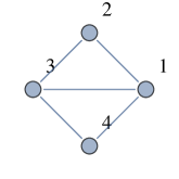
(a)

(b)

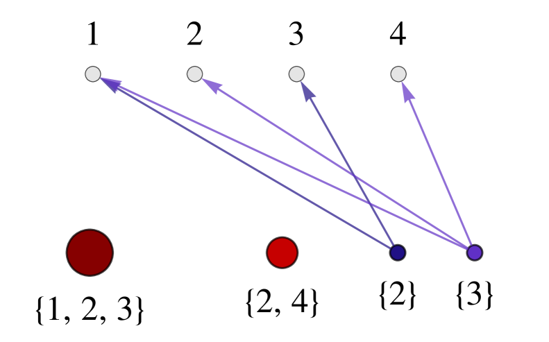
$\gamma\in\Gamma_{G}$ $\left\{1,2,3\right\}$ $\left\{2,4\right\}$ $\mathcal{K}_{G}$ $\left\{\left\{2\right\},\left\{3\right\}\right\}$ $v_{i_{1}}$ $1$ $2$ $\xi\in\left\langle\mathcal{K}_{G}\right\rangle$ $\emptyset$ $\left\{2\right\}$ $\left\{3\right\}$ $\left\{2,3\right\}$ $\pi_{G}\left(\gamma\right)$ $-1$ $1$ $\pi_{G}\left(\xi\right)$ $1$ $1$ $1$ $-1$ $x_{\Gamma}$ $\left\{1\right\}$ $i^{(c_{\xi})}$ $0$ $1010$ $1101$ $0111$ $|i^{(x_{\Gamma})}\rangle$ $|1000\rangle$ $\ket{\psi_{\emptyset}\left(\xi\right)}$ $|1000\rangle$ $|0010\rangle$ $|0101\rangle$ $-|1111\rangle$

(c)

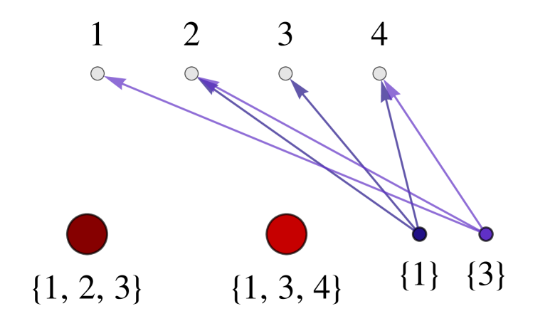
$\gamma\in\Gamma_{G}$ $\left\{2,1,3\right\}$ $\left\{4,1,3\right\}$ $\mathcal{K}_{G}$ $\left\{\left\{1\right\},\left\{3\right\}\right\}$ $v_{i_{1}}$ $2$ $4$ $\xi\in\left\langle\mathcal{K}_{G}\right\rangle$ $\emptyset$ $\left\{1\right\}$ $\left\{3\right\}$ $\left\{1,3\right\}$ $\pi_{G}\left(\gamma\right)$ $-1$ $-1$ $\pi_{G}\left(\xi\right)$ $1$ $1$ $1$ $-1$ $x_{\Gamma}$ $\left\{2,4\right\}$ $i^{(c_{\xi})}$ $0$ $0111$ $1101$ $1010$ $|i^{(x_{\Gamma})}\rangle$ $|0101\rangle$ $\ket{\psi_{\emptyset}\left(\xi\right)}$ $|0101\rangle$ $|0010\rangle$ $|1000\rangle$ $-|1111\rangle$

(d)

Figure 2: (Color online) Example for the determination of X-chain states (see section IV for details). (a) The graph state $|K_{4}^{\neg 1}\rangle$. (b) The factorization diagram of $|K_{4}^{\neg 1}\rangle$ (for an explanation, see Algorithm 14). (c),(d) The incidence structure of the X-chain generators and correlation group generators of $|K_{4}^{\neg 1}\rangle$. The choices of these generators are not unique, and lead to different fundamental X-chain states $\ket{i^{(x_{\Gamma})}}$. However, they arrive at the identical set of X-chain states $\{\ket{\psi_{\emptyset}(\xi)},\xi\in\braket{\mathcal{K}_{G}}\}$.

Let us illustrate these concepts by an example, the graph state $|K_{4}^{\neg 1}\rangle$ (Fig. 2a), which corresponds to the graph with one edge missing from the complete graph $K_{4}$. Its X-chain generators can be chosen as $\Gamma_{G}=\left\{\gamma_{1},\gamma_{2}\right\}=\left\{\left\{1,2,3\right\},\left\{2,4\right\}\right\}$ (see Fig. 2c). The exclusive vertex $v_{1}$ for $\gamma_{1}$ can be chosen as $1$, while $v_{2}$ for $\gamma_{2}$ is $4$. Only $\gamma_{1}$ has negative parity, and therefore $x_{\Gamma}=\left\{1\right\}$ and the fundamental X-chain state is $\ket{i^{(x_{\Gamma})}}=|1000\rangle$.

From the fundamental X-chain state $\ket{i^{(x_{\Gamma})}}$ one can derive all the X-chain states and correlation states with the following proposition.

Proposition 11 (Form of X-chain states, $\mathcal{K}$-correlation states).

Let $\xi\in\left\langle\mathcal{K}_{G}\right\rangle$ be an X-resource and $\left\langle\mathcal{K}\right\rangle\subseteq\left\langle\mathcal{K}_{G}\right\rangle$. An X-chain state is given as

$$|\psi_{\emptyset}\left(\xi\right)\rangle=\pi_{G}\left(\xi\right)\left|i^{(x_{\Gamma})}\oplus i^{(c_{\xi})}\right\rangle,$$ (28)

where $\pi_{G}\left(\xi\right)$ is the stabilizer parity of $\xi$ (see Eq. (13)), and $c_{\xi}$ is the correlation index of $\xi$.

A $\mathcal{K}$-correlation state is the superposition of X-chain states,

$$|\psi_{\mathcal{K}}\left(\xi\right)\rangle=\frac{1}{2^{\left|\mathcal{K}\right|/2}}\sum_{\xi^{\prime}\in\left\langle\mathcal{K}\right\rangle}|\psi_{\emptyset}\left(\xi\Delta\xi^{\prime}\right)\rangle.$$ (29)

Proof.

See Appendix A. ∎

According to this proposition, the X-chain states of $\ket{K_{4}^{\lnot 1}}$ derived from $\ket{i^{(x_{\gamma})}}=\ket{1000}$ are given in the table in Fig. 2c. Alternatively, one can also choose the X-chain generators $\Gamma_{G}=\left\{\gamma_{1},\gamma_{2}\right\}=\left\{\left\{2,1,3\right\},\left\{4,1,3\right\}\right\}$ (see Fig. 2d). In this case $v_{1}=2$ and $v_{2}=4$. The parities of $\gamma_{1}$ and $\gamma_{2}$ are both negative, hence $|i^{(x_{\Gamma})}\rangle=|0101\rangle$. However, the sets of obtained X-chain states $\Psi^{(\emptyset)}$ are identical in both cases.

The correlation states $|\psi_{\mathcal{K}}\left(\xi\right)\rangle$ are then the superposition of their corresponding X-chain states. For example, in Fig. 2c the correlation state $|\psi_{\{\{2,3\}\}}\left(\emptyset\right)\rangle=(\ket{1000}-\ket{1111})/\sqrt{2}$. The correlation states have the following properties.

Corollary 12 (Properties of $\mathcal{K}$-correlation states).

Let $\braket{\mathcal{K}}\subseteq\braket{\mathcal{K}_{G}}$ be a correlation index subgroup, then

1. $|\psi_{\mathcal{K}}\left(\xi\right)\rangle$ is stabilized by all stabilizers $s_{G}^{(\kappa)}$ with $\kappa\in\left\langle\Gamma_{G}\right\rangle\times\left\langle\mathcal{K}\right\rangle$

   $$s_{G}^{(\kappa)}|\psi_{\mathcal{K}}\left(\xi\right)\rangle=|\psi_{\mathcal{K}}\left(\xi\right)\rangle.$$ (30)

   Therefore the space $\mathrm{span}(\Psi^{(\mathcal{K})})$, see Eq. (26), is also stabilized by $s_{G}^{(\kappa)}$ with $\kappa\in\left\langle\Gamma_{G}\right\rangle\times\left\langle\mathcal{K}\right\rangle$.

2. For $\xi_{1}\in\left\langle\mathcal{K}_{G}\right\rangle$ and $\xi_{1}\not\in\left\langle\mathcal{K}\right\rangle$, it holds that

   $$s_{G}^{(\xi_{1})}|\psi_{\mathcal{K}}\left(\xi_{2}\right)\rangle=|\psi_{\mathcal{K}}\left(\xi_{1}\Delta\xi_{2}\right)\rangle.$$ (31)

3. For $\kappa\in\mathcal{K}_{G}$ and $\kappa\not\in\mathcal{K}$, the $\mathcal{K}\cup\left\{\mathcal{\kappa}\right\}$-correlation state can be obtained by

   $$|\psi_{\mathcal{K}\cup\{\kappa\}}\left(\xi\right)\rangle=\frac{1+s_{G}^{(\kappa)}}{\sqrt{2}}|\psi_{\mathcal{K}}\left(\xi\right)\rangle.$$ (32)

Proof.

See Appendix A. ∎

With these properties one can derive the representation of graph states in the X-basis.

Theorem 13 (X-chain state representation of graph states).

Let $|G\rangle$ be a graph state. Then $|G\rangle$ is a $\mathcal{K}_{G}$-correlation state, which is a superposition of X-chain states $|\psi_{\emptyset}\left(\xi\right)\rangle$, i.e.

$$|G\rangle=|\psi_{\mathcal{K}_{G}}\rangle=\frac{1}{2^{\left|\mathcal{K}_{G}\right|/2}}\sum_{\xi\in\left\langle\mathcal{K}_{G}\right\rangle}|\psi_{\emptyset}\left(\xi\right)\rangle.$$ (33)

Proof.

According to property 1 in Corollary 12, one can infer that $\ket{\psi_{\mathcal{K}_{G}}}$ is stabilized by all graph state stabilizers $s_{G}^{(\xi)}$ with $\xi\in\left\langle\Gamma_{G}\right\rangle\times\left\langle\mathcal{K}_{G}\right\rangle$. As a result of Lemma 8, $\ket{\psi_{\mathcal{K}_{G}}}$ is stabilized by the whole graph state stabilizer group $\mathcal{S}_{G}$. According to the definition of graph states in the stabilizer formalism, one can infer that $|G\rangle=\ket{\psi_{\mathcal{K}_{G}}}$. The explicit form of $\ket{\psi_{\mathcal{K}_{G}}}$ in Eq. (33) is obtained by Proposition 11. ∎

Note that the graph state obtained by this theorem may differ from the real one by a global phase $-1$, i.e. $\ket{G}=-\ket{\psi_{\mathcal{K}_{G}}}$ . We summarize the approach of X-chain factorization of a graph state representation in a so-called factorization diagram.

Algorithm 14 (Factorization diagram).

The X-chain factorization of graph states can be described in the factorization diagram shown in Fig. 3.

1. One decomposes the group $\mathcal{P}(V_{G})$ into the direct product of the X-chain group $\braket{\Gamma_{G}}$ and the correlation group $\braket{\mathcal{K}_{G}}$ (Lemma 8).

2. From the X-chain group $\braket{\Gamma_{G}}$, one obtains the set of X-chain states $\Psi^{\emptyset}_{\mathcal{K}_{G}}$ (Proposition 10).

3. From the correlation group $\braket{\mathcal{K}_{G}}$, one obtains graph states via the superposition of the X-chain states in $\Psi^{\emptyset}_{\mathcal{K}_{G}}$ (Theorem 13).

Figure 3: (Color online) X-chain factorization diagram of graph states: A graphical summary of Proposition 10, 11 and Theorem 13. This diagram illustrates the algorithm for representing a graph state in the X-basis.

The arrows in the factorization diagram can be interpreted as a mapping from the sets of X-resources to their corresponding stabilized Hilbert subspaces. As we already discussed at the end of the section II, a graph state is mapped from the powerset of vertices by stabilizer induction, which is depicted in the left hand side of the equality in the diagram. The equation in the first row is the X-chain factorization of the group $(\mathcal{P}(V_{G}),\Delta)$ (Lemma 8). The arrow from the X-chain group $\Gamma_{G}$ to the X-chain states $\Psi^{(\emptyset)}$ interprets the mapping from the X-chain group to the stabilized subspace spanned by $\Psi^{(\emptyset)}$ (Definition 9 and Proposition 10). The arrow from the correlation group $\langle\mathcal{K}_{G}\rangle$ through the X-chain states $\Psi^{(\emptyset)}$ to the $\mathcal{K}_{G}$-correlation state is a mapping from the subspace $\mathrm{span}(\Psi^{(\emptyset)})$ to the $\mathcal{K}_{G}$-correlation state $|\psi_{\mathcal{K}_{G}}\rangle$, which is stabilized by the $\mathcal{K}_{G}$-stabilizers. This arrow-represented mapping is the summation (superposition) of the X-chain states over the correlation group $\braket{\mathcal{K}_{G}}$ (Proposition 11). Since the graph state $\ket{G}$ is the only stabilized state of the stabilizers induced by the group $\braket{\Gamma_{G}}\times\braket{\mathcal{K}_{G}}$, it is identical to the $\mathcal{K}_{G}$-correlation state $|\psi_{\mathcal{K}_{G}}\rangle$ (Theorem 13), which is represented by the equality of the last line in the factorization diagram. With the help of the factorization diagram in Fig. 2b, the graph state $|K_{4}^{\lnot 1}\rangle$ is given by

$$|K_{4}^{\lnot 1}\rangle=\frac{1}{2}\left(\left|1000\right\rangle+\left|0010\right\rangle+\left|0101\right\rangle-\left|1111\right\rangle\right).$$ (34)

Since the edge number $|E_{G[\xi]}|$ is identical to the product $\langle i_{Z}^{(\xi)},i_{Z}^{(\xi)}\rangle_{A_{G}}$ in Eq. (10), according to the definition of the stabilizer-parity (Def. 4),

$$\pi_{G}\left(\xi\right)=(-1)^{\langle i_{Z}^{(\xi)},i_{Z}^{(\xi)}\rangle_{A_{G}}}.$$ (35)

Hence the representation of graph states in the Z-basis in Eq. (10) can be reformulated as

$$|G\rangle=\frac{1}{2^{n/2}}\sum_{\xi\subseteq V_{G}}\pi_{G}\left(\xi\right)|i_{Z}^{(\xi)}\rangle.$$ (36)

Comparing this Z-representation with the representation of a graph state in the X-basis given in Eq. (33), the number of terms in the representation is reduced from $2^{|V_{G}|}$ to $2^{|\mathcal{K}_{G}|}$. The correlation group $\braket{\mathcal{K}_{G}}$ can be directly obtained if one knows the X-chain group. The X-chain group can be searched by a criterion that the cardinality of the intersection of the vertex neighborhood with the X-chain $|N_{v}\cap\xi|$ should be even for all $v\in V_{G}$ WuKampermannBruss2015-XChainAlgo . The search of the X-chains of a graph state $\ket{G}$ is equivalent to finding the 2-modulus-kernel of the adjacency matrix of the graph $G$. As this is efficient, the representation of graph states in the X-basis is feasible. The larger the X-chain group that a graph state possesses, the smaller is its correlation group and hence the more efficient is its X-chain factorization.

Note that not every graph state has non-trivial X-chains (non-trivial means not the empty set). For graph states without non-trivial X-chains, their X-chain factorization contains all X-basis states, and thus has the same difficulty as their Z-representation.

Besides, the X-chain factorization of graph states in Theorem 13 implies that the possible outcomes of X-measurements are only the X-chain states, $|\psi_{\emptyset}\left(\xi\right)\rangle$. Consequently two graph states with different X-chains can have different X-chain states, and hence are distinguishable via the X-measurement outcomes. In Table 3, we list the X-chain generators and X-chain states of graph states with $3$ vertices. Since the X-chain states of these graph states are different from each other, one can therefore distinguish these $8$ graph states via local X-measurements with non-zero probability of success.

$\ket{G}$	$\Gamma_{G}$	$\Psi^{(\emptyset)}_{\mathcal{K}_{G}}=\{\ket{\psi_{\emptyset}(\xi)}:\xi\in\braket{\mathcal{K}_{G}}\}$
	$\left\{\{1\},\{2\},\{3\}\right\}$	$\left\{\left|000\right\rangle\right\}$
	$\left\{\{3\}\right\}$	$\left\{\ket{000},\ket{010},\ket{100},-\ket{110}\right\}$
	$\left\{\{2\}\right\}$	$\left\{\ket{000},\ket{001},\ket{100},-\ket{101}\right\}$
	$\left\{\{1\}\right\}$	$\left\{\ket{000},\ket{001},\ket{010},-\ket{011}\right\}$
	$\left\{\{2,3\}\right\}$	$\left\{\ket{000},\ket{100},\ket{011},-\ket{111}\right\}$
	$\left\{\{1,3\}\right\}$	$\left\{\ket{000},\ket{100},\ket{101},-\ket{111}\right\}$
	$\left\{\{1,2\}\right\}$	$\left\{\ket{000},\ket{001},\ket{110},-\ket{111}\right\}$
	$\left\{\{1,2,3\}\right\}$	$\left\{\left|100\right\rangle,\left|010\right\rangle,\left|001\right\rangle,-\left|111\right\rangle\right\}$

Table 3: X-chain states of 3-vertex graph states

V Application of the X-chain factorization

The representation of graph states in the X-chain factorization reveals certain substructures of graph states. In this section, we discuss its usefulness for the calculation of graph state overlaps, the Schmidt decomposition and unilateral projections in bipartite systems.

V.1 Graph state overlaps

In WuRKSKMBruss2014-05 , the overlaps of graph states are the basis for genuine multipartite entanglement detection of randomized graph states with projector-based witnesses $W_{G}=\mathbbm{1}/2-\ket{G}\bra{G}$, see AcinBLSanpera2001-07 ; GuhneHBELMSanpera2002-12 , where $G$ is a connected graph. An expectation value $\mathrm{tr}(|H\rangle\langle H|G\rangle\langle G|)>1/2$ indicates the presence of genuine multipartite entanglement of the graph state $\ket{H}$.

In general, a graph state $|G\rangle=\prod_{e\in E_{G}}U_{Z}^{(e)}|0_{X}\rangle$ is created by control-Z operators $U_{Z}^{(e)}$, where

$$U_{Z}^{\{v_{a},v_{b}\}}:=\ket{0}\bra{0}^{(a)}\otimes\mathbbm{1}^{(b)}+\ket{1}\bra{1}^{(a)}\otimes\sigma_{Z}^{(b)}.$$ (37)

Since the operators $U_{Z}^{(e)}$ commute for different edges $e$ and are unitary and Hermitian, the overlap $\braket{G}{H}$ is calculated by

$$\left\langle G|H\right\rangle=\langle 0^{\otimes n}_{X}|\prod_{e\in E_{G}\Delta E_{H}}U_{Z}^{(e)}|0^{\otimes n}_{X}\rangle=\langle 0^{\otimes n}_{X}|G\Delta H\rangle.$$ (38)

According to Eq. (10),

$$\langle G|H\rangle=\frac{1}{2^{n/2}}\sum_{i=0}^{2^{n}-1}\left(-1\right)^{\left\langle i_{Z},i_{Z}\right\rangle_{A_{G\Delta H}}},$$ (39)

where $G\Delta H$ is the symmetric difference of the graphs $G$ and $H$. $G\Delta H$ is the graph $(V_{G\Delta H},E_{G\Delta H})$, whose vertices and edges are $V_{G\Delta H}=V_{G}=V_{H}$ and $E_{G\Delta H}=E_{G}\cup E_{H}\setminus E_{G}\cap E_{H}$, respectively. However, the complexity of this calculation increases exponentially with the size of the system.

The quantity obtained from Eq. (10),

$$\left\langle 0^{\otimes n}_{X}|G\right\rangle=\frac{1}{2^{n/2}}\sum_{i=0}^{2^{n}-1}\left(-1\right)^{\left\langle i_{Z},i_{Z}\right\rangle_{A}},$$ (40)

corresponds to the difference of the positive and negative amplitudes of $\ket{G}$ in the Z-basis. We can define for each graph state $\ket{G}$ a Boolean function $f_{G}:=\braket{i_{Z},i_{Z}}_{A}\pmod{2}$ with $A$ being the adjacency matrix. The function $f_{G}$ is balanced, if and only if $\braket{0^{\otimes n}_{X}}{G}=0$, otherwise it is biased. We introduce the bias degree of a graph state and define its Z-balance as follows.

Definition 15 (Bias degree and Z-balanced graph states).

The (Z-)bias degree $\beta$ of a graph state $|G\rangle$ with $n$ vertices is defined as the overlap

$$\beta(|G\rangle):=\langle 0_{X}^{\otimes n}|G\rangle,$$ (41)

where $|0_{X}\rangle=\left(|0_{Z}\rangle+|1_{Z}\rangle\right)/\sqrt{2}$. A graph state with zero bias degree is called Z-balanced. β(—G⟩)

The bias degree is related to the weight of a graph state, $\omega^{-}\left(G\right):=\left|\left\{i_{Z}:\langle i_{Z}|G\rangle/\left|\langle i_{Z}|G\rangle\right|=-1\right\}\right|$, which is equal to the number of minus amplitudes in $|G\rangle$ in the Z-basis CosentinoSimone2009-Weight . The probability of finding a negative amplitude in the Z-basis is $1/2-\beta(|G\rangle)/2$, which is equal to $\omega^{-}\left(G\right)/2^{n}$. Note that as a result of Eq. (36), the bias degree of a graph state is equal to the sum of its stabilizer parities.

$$\beta(\ket{G})=\sum_{\xi\subseteq V_{G}}\pi_{G}(\xi).$$ (42)

As a result of Theorem 13, the bias degree $\Braket{0_{x}}{G}$, depends only on the number of X-chain generators and the parity of their corresponding X-resources.

Corollary 16 (Graph state overlaps and bias degrees).

The overlap of two graph states $\ket{G}$ and $\ket{H}$ is equal to the bias degree of the graph state $\ket{G\Delta H}$, i.e.

$$\braket{G}{H}=\beta(\ket{G\Delta H}).$$ (43)

The bias degree of a graph state $|G\rangle$ is equal to

$$|\beta(|G\rangle)|=\frac{1}{2^{\left(n-\left|\Gamma_{G}\right|\right)/2}}\prod_{\gamma\in\Gamma_{G}}\delta_{\pi_{G}(\gamma)}^{1},$$ (44)

where $\Gamma_{G}$ is the X-chain generating set of $|G\rangle$, $\delta$ is the Kronecker-delta and $\pi_{G}(\gamma)$ is the stabilizer-parity of X-chain generators $\gamma$.

Proof.

First we prove that there does not exist $\xi$ such that $c_{\xi}=x_{\Gamma}$. Assume $c_{\xi}=x_{\Gamma}$, then $|c_{\xi}\cap\gamma|\overset{\operatorname{mod}2}{=}|\xi\cap c_{\gamma}|=0$. However, according to the definition of $x_{\Gamma}$ (Def. 10), $|c_{\xi}\cap\gamma|=|x_{\Gamma}\cap\gamma|=1$ which contradicts $|c_{\xi}\cap\gamma|=0\operatorname{mod}2$. Then the only possible zero X-chain state is $\ket{i^{x_{(\Gamma)}}}$. Therefore Theorem 13 leads to

$$|\beta(|G\rangle)|=\frac{1}{2^{\left(n-\left|\Gamma_{G}\right|\right)/2}}\langle 0_{X}|i^{(x_{\Gamma})}\rangle.$$ (45)

According to the definition of the X-chain basis, $x_{\Gamma}=\emptyset$ if and only if $\pi_{G}\left(\gamma\right)=1$ for all X-chain generators $\gamma\in\Gamma_{G}$, that means $\left\langle 0_{X}|i^{(x_{\Gamma})}\right\rangle=\prod_{\gamma\in\Gamma_{G}}\delta_{\pi_{G}(\gamma)}^{1}$. ∎

In CosentinoSimone2009-Weight , the authors relate the weight $\omega^{-}\left(G\right)$ to the binary rank of the adjacency matrix of graphs. Our Corollary 16 is a similar result showing that the bias degree depends on the binary rank of the adjacency matrix, which is equal to $n-\left|\Gamma_{G}\right|$.

Here, we focus on the bias degree and Z-balance of graph states. Since the X-chain group of a graph state can be efficiently determined, instead of Eq. (39), Corollary 16 provides an efficient method to calculate the graph state overlap. As a result of Corollary 16, we arrive at the following corollary.

Corollary 17 (Z-balanced graph states).

A graph state is Z-balanced, if and only if it has at least one X-chain generator $\gamma^{-}$ with negative stabilizer-parity, i.e. $\left|E\left(G\left[\gamma^{-}\right]\right)\right|$ is odd. Two graph states are orthogonal, if and only if $|G\Delta H\rangle$ is Z-balanced.

Knowing all the Z-balanced graph states with vertex number $n$ allows one to identify all pairs of orthogonal graph states with $n$ vertices. Note that relabeling a graph state (graph isomorphism) does not change its bias degree, since the structure of the X-chain group does not change under graph isomorphism.

In Fig. 4, the Z-balanced graph states up to five vertices are listed. Every graph in the figure represents an isomorphic class. From these balanced graph states one can obtain orthogonal graph states via the graph symmetric difference. Examples of orthogonal graph states derived from the Z-balanced graph states $|C_{3}\rangle$ and $|C_{5}\rangle$ are shown in Figs. 5 and 6 , respectively, ($C_{3}$ and $C_{5}$ are the first and fifth graph in Fig. 4 ).

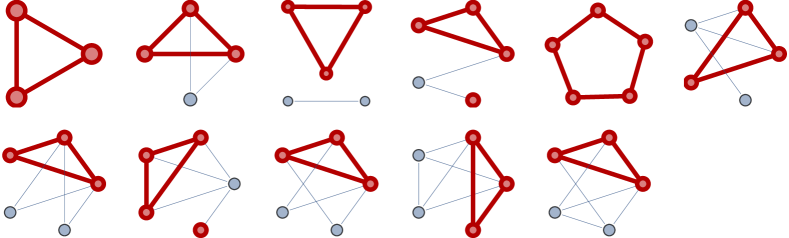
Figure 4: (Color online) Z-balanced graph states (see Def. 15) up to $5$ vertices: Each graph represents a graph isomorphic class. Each balanced graph state has at least one X-chain $\gamma^{-}$ with negative parity. In each graph, the $\gamma^{-}$-induced subgraph $G[\gamma^{-}]$ is highlighted in red with bold edges. Every highlighted $\gamma^{-}$-induced subgraph has an odd edge number.

Figure 5: Orthogonal graph states derived from the Z-balanced graph state $|C_{3}\rangle$: The graph states in each cell are orthogonal to each other. Their symmetric difference is identical to the cycle graph $C_{3}$, where $C_{3}$ is the first graph in Fig. 4.

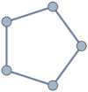
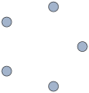
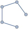
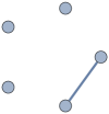
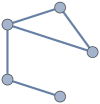
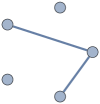
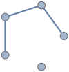
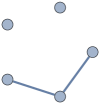
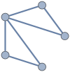
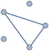
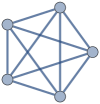
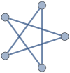
Figure 6: Orthogonal graph states derived from the Z-balanced graph state $|C_{5}\rangle$: The graph states in each cell are orthogonal. Their symmetric difference is identical to the cycle graph $C_{5}$, where $C_{5}$ is the fifth graph in Fig. 4.

V.2 Schmidt decomposition

In this section, we discuss the Schmidt decomposition of graph states represented in the X-basis, which is derived via the X-chain factorization. The Schmidt decomposition of a graph state for an $A|B$-bipartition reads

$$|G\rangle=\frac{1}{2^{r_{S}/2}}\sum_{i=1}^{r_{S}}\ket{\phi_{i}^{(A)}}\ket{\psi_{i}^{(B)}},$$ (46)

where $\braket{\phi_{i}^{(A)}}{\phi_{j}^{(A)}}=\delta_{ij}$ and $\braket{\psi_{i}^{(B)}}{\psi_{j}^{(B)}}=\delta_{ij}$. r_S Here $r_{S}$ is the Schmidt rank of the graph state $|G\rangle$ with respect to the partition $A$ versus $B$. Its value

$$r_{S}=\left|S_{A}\right|:=\left|\left\{s_{G}^{(\xi)}\in S_{G}:\text{supp}(s_{G}^{(\xi)})\subseteq A\right\}\right|$$ (47)

is studied in the section III.B of Ref. HeinEisertBriegel2004-06 via the Schmidt decomposition of graph states in the Z-basis, where $\mathrm{supp}(s_{G}^{(\xi)})$ is the support of the stabilizer $s_{G}^{(\xi)}$. The $\mathrm{supp}(s_{G}^{(\xi)})$ is equal to the projection on the Hilbert space spanned by qubits corresponding to the vertices $\xi\cup c_{\xi}$, which is the set of vertices on which the stabilizer $s_{G}^{(\xi)}$ acts non-trivially (i.e. not equal to the identity).

We derive the Schmidt decomposition of graph states in the X-basis in the following steps. First, we generalize the X-chain factorization of graph states (Theorem 13) to the X-chain factorization of arbitrary correlation states (Theorem 18). Second, we introduce three correlation subgroups, whose correlation states are $A|B$-biseparable (Lemma 20). Third, we prove the orthonormality of these correlation states (Lemma 21). At the end, we arrive at the Schmidt decomposition in Theorem 22.

The X-chain factorization of graph states in Theorem 13 can be generalized to correlation states (introduced in Eqs. (25) and (29)) as follows.

Theorem 18 (X-chain factorization of $\mathcal{K}$-correlation states).

Let $\left\langle\mathcal{K}_{1}\right\rangle,\left\langle\mathcal{K}_{2}\right\rangle\subseteq\left\langle\mathcal{K}_{G}\right\rangle$ be two disjoint correlation subgroups of a graph state $|G\rangle$, and $\mathcal{K}=\mathcal{K}_{1}\cup\mathcal{K}_{2}$. Then the $\mathcal{K}$-correlation state is a superposition of $\mathcal{K}_{1}$-correlation states,

$$|\psi_{\mathcal{K}}\left(\xi\right)\rangle=\frac{1}{2^{\left|\mathcal{K}_{2}\right|/2}}\sum_{\xi^{\prime}\in\left\langle\mathcal{K}_{2}\right\rangle}|\psi_{\mathcal{K}_{1}}\left(\xi\Delta\xi^{\prime}\right)\rangle$$ (48)

with $\xi\in\braket{\mathcal{K}_{G}}/\braket{\mathcal{K}}$ being an element in their quotient group. Theorem 13 is a special case of this theorem related by $\braket{\mathcal{K}}=\left\langle\mathcal{K}_{1}\right\rangle\times\left\langle\mathcal{K}_{2}\right\rangle=\mathcal{\emptyset}\times\left\langle\mathcal{K}_{G}\right\rangle$.

Proof.

According to the definition in Eq. (25) it holds

$$|\psi_{\mathcal{K}_{1}\cup\mathcal{K}_{2}}\left(\xi\right)\rangle=s_{G}^{(\xi)}\prod_{\kappa\in\mathcal{K}_{2}}\frac{1+s_{G}^{(\kappa)}}{\sqrt{2}}\prod_{\kappa\in\mathcal{K}_{1}}\frac{1+s_{G}^{(\kappa)}}{\sqrt{2}}\left|i^{(x_{\Gamma})}\right\rangle.$$ (49)

Due to the commutativity of the graph state stabilizers it follows

$$|\psi_{\mathcal{K}}\left(\xi\right)\rangle=|\psi_{\mathcal{K}_{1}\cup\mathcal{K}_{2}}\left(\xi\right)\rangle=\prod_{\kappa\in\mathcal{K}_{2}}\frac{1+s_{G}^{(\kappa)}}{\sqrt{2}}|\psi_{\mathcal{K}_{1}}\left(\xi\right)\rangle.$$ (50)

According to Proposition 2, $s_{G}^{(\kappa_{1}\Delta\kappa_{2})}=s_{G}^{(\kappa_{1})}s_{G}^{(\kappa_{2})}$, the product of $(1+s_{G}^{(\kappa)})$ with $\kappa\in\mathcal{K}_{2}$ becomes the sum of the stabilizers $s_{G}^{(\xi^{\prime})}$ with $\xi^{\prime}\in\left\langle\mathcal{K}_{2}\right\rangle$.

$$|\psi_{\mathcal{K}}\left(\xi\right)\rangle =\frac{1}{2^{\left|\mathcal{K}_{2}\right|/2}}\sum_{\xi^{\prime}\in\left\langle\mathcal{K}_{2}\right\rangle}s_{G}^{(\xi^{\prime})}|\psi_{\mathcal{K}_{1}}\left(\xi\right)\rangle$$

$$=\frac{1}{2^{\left|\mathcal{K}_{2}\right|/2}}\sum_{\xi^{\prime}\in\left\langle\mathcal{K}_{2}\right\rangle}|\psi_{\mathcal{K}_{1}}\left(\xi\Delta\xi^{\prime}\right)\rangle,$$ (51)

where the second equality is a result of property 2 in Corollary 12. ∎

Algorithm 19 (Factorization diagram of correlation states).

Theorem 18 can be interpreted by the factorization diagram in Fig. 7.

1. One decomposes the group $\mathcal{P}(V_{G})$ into the direct product of the X-chain group $\braket{\Gamma_{G}}$ and the correlation group $\braket{\mathcal{K}_{G}}$.

2. From the X-chain group $\braket{\Gamma_{G}}$, one obtains the set of X-chain states $\Psi^{\emptyset}_{\mathcal{K}_{G}}$.

3. From the correlation group $\braket{\mathcal{K}_{1}}$, one obtains graph states via the superposition of the X-chain states in $\Psi^{\emptyset}_{\mathcal{K}_{G}}$ within $\braket{\mathcal{K}_{1}}$.

4. At the end the correlation state $\ket{\psi_{\mathcal{K}_{1}\cup\mathcal{K}_{2}}(\xi)}$ is the superposition of the $\mathcal{K}_{1}$-correlation states $\ket{\psi_{\mathcal{K}_{1}}(\xi\Delta\xi^{\prime})}\in\Psi^{(\mathcal{K}_{1})}_{\mathcal{K}_{G}}$ inside the correlation group $\xi^{\prime}\in\braket{\mathcal{K}_{2}}$ (Theorem 18).

Figure 7: (Color online) The X-chain factorization diagram of correlation states: A graphical summary of Theorem 18. The $\xi$ in $|\psi_{\mathcal{K}_{1}\cup\mathcal{K}_{2}}\left(\xi\right)\rangle$ are elements in the quotient group, $\xi\in\braket{\mathcal{K}_{G}}/\braket{\mathcal{K}_{1}\cup\mathcal{K}_{2}}$.

The subspace of X-chain states $\mathrm{span}(\Psi_{K_{G}}^{(\emptyset)})$ are projected via $\braket{\mathcal{K}_{1}}$-stabilizers to the space spanned by the $\mathcal{K}_{1}$-correlation states $|\psi_{\mathcal{K}_{1}}\left(\xi\right)\rangle$. Further, the subspace $\mathrm{span}(\Psi_{K_{G}}^{(\mathcal{K}_{1})})$ are then projected via $\braket{\mathcal{K}_{2}}$-stabilizers to the $\mathcal{K}_{1}\cup\mathcal{K}_{2}$-correlation states $|\psi_{\mathcal{K}_{1}\cup\mathcal{K}_{2}}\left(\xi\right)\rangle$. With this theorem, one can obtain the Schmidt decomposition of graph states, by appropriate selection of the correlation subgroup $\mathcal{K}_{1}$, such that its corresponding $\mathcal{K}_{1}$-correlation states are $A|B$-separable and mutually orthonormal.

Let $|G\rangle$ be a graph state with the correlation group $\left\langle\mathcal{K}_{G}\right\rangle$ and $A|B$ be a bipartition of its vertices. In order to find the Schmidt decomposition, we select $\braket{K_{1}}$ as the union of three disjoint correlation subgroups specified as follows.

1. The correlation subgroup, whose elements possess a correlation index only in $B$:

   $$\langle\mathcal{K}^{(B)}\rangle:=\left\{\xi\in\left\langle\mathcal{K}_{G}\right\rangle:c_{\xi}\subseteq B\right\}.$$ (52)

   ⟨K^(B)⟩

2. The correlation subgroup, whose elements possess a correlation index only in $A$ and only consists of vertices in $A$:

   $$\langle\mathcal{K}_{A}^{(A)}\rangle:=\left\{\xi\in\left\langle\mathcal{K}_{G}\right\rangle:c_{\xi}\subseteq A,\xi\subseteq A\right\}.$$ (53)

   ⟨K_A^(A)⟩

3. The correlation subgroup, whose elements possess a correlation index only in $A$, consists of vertices in $B$ and has an even number of edges between all $\beta\in\left\langle\mathcal{K}^{(B)}\right\rangle$:

   $$\langle\mathcal{K}_{\sim B}^{(A)}\rangle :=\left\{\xi\in\left\langle\mathcal{K}_{G}\right\rangle:c_{\xi}\subseteq A,\xi\not\subseteq A\right\}\cap\{\xi\in\left\langle\mathcal{K}_{G}\right\rangle:$$

   $$\left|E_{G}\left(\xi:\beta\right)\right|\overset{\operatorname{mod}2}{=}0\text{, for all }\beta\in\left\langle\mathcal{K}^{(B)}\right\rangle\}.$$ (54)

   ⟨K_∼B^(A)⟩

These three groups form a special group

$$\langle\mathcal{K}^{A\rfloor B}\rangle:=\langle\mathcal{K}_{A}^{(A)}\cup\mathcal{K}_{\sim B}^{(A)}\rangle\times\langle\mathcal{K}^{(B)}\rangle$$ (55)

called $A\rfloor B$-correlation group. ⟨K^A⌋B⟩—ψ_A⌋B(ξ)⟩ (The notation “$A\rfloor B$” is used, as the group is not symmetric with respect to exchanging $A$ and $B$.) We will show in Lemma 20 that all $A\rfloor B$-correlation states $|\psi_{\mathcal{K}^{A\rfloor B}}(\xi)\rangle$ with $\xi\in\left\langle\mathcal{K}_{G}\right\rangle/\langle\mathcal{K}^{A\rfloor B}\rangle$, are $A|B$-separable. The corresponding quotient group is denoted as

$$\langle\mathcal{K}^{A\rightharpoonup B}\rangle:=\left\langle\mathcal{K}_{G}\right\rangle/\langle\mathcal{K}^{A\rfloor B}\rangle$$ (56)

and called $\left(A\rightharpoonup B\right)$-correlation group. ⟨K^A↼B⟩ (The notation $A\rightharpoonup B$ is introduced, as there is again no symmetry under exchange of $A$ and $B$, as the correlation index $c_{\xi}$ of $\xi\in\braket{\mathcal{K}^{A\rightharpoonup B}}$ is always inside $A$.) We will show in Theorem 22 that the Schmidt rank of $\ket{G}$ is equal to the cardinality $|\braket{\mathcal{K}^{A\rightharpoonup B}}|$. That means that the correlation subgroup $\mathcal{K}^{A\rightharpoonup B}$ generates the $A|B$ correlation in the graph state $\ket{G}$. Note that we investigated many graphs and found their correlation subgroups $\langle\mathcal{K}_{\sim B}^{(A)}\rangle$ all to be empty. That means the group $\langle\mathcal{K}_{\sim B}^{(A)}\rangle$ may not exist for any graph state. However, this is still an open question.

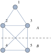
(a)

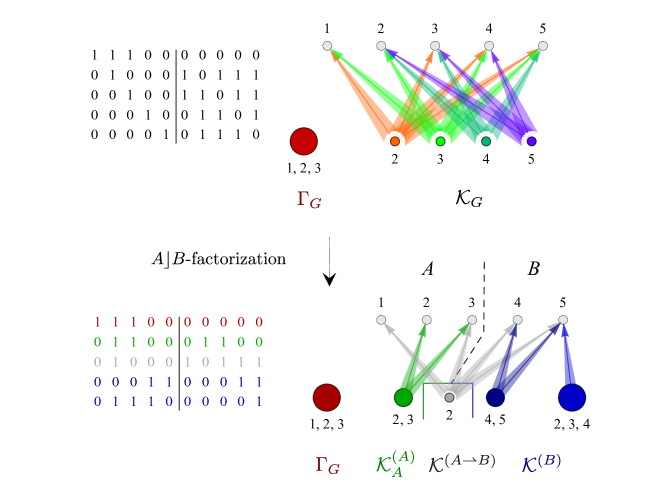
(b)

(c)

Figure 8: (Color online) $A\rfloor B$-factorization of graph states: (a) The graph state $\ket{G_{\mathrm{House}}}$ corresponding to a “St. Nicholas’s house” is divided in two subsystems $A=\{1,2,3\}$ and $B=\{4,5\}$. (b) The binary representation of the X-chain factorization (the upper row) and $A\rfloor B$-factorization (the lower row). (c) The $A\rfloor B$-factorization diagram (see Algorithm 23) of the “St. Nicholas’s house” graph state $\ket{G_{\mathrm{House}}}$.

In this $A\rfloor B$-factorization, the correlation group $\mathcal{K}_{G}$ is divided into four subgroups. Let us take the graph of “St. Nicholas’s house” in Fig. 8a as an example. This “house” state $|G_{\mathrm{House}}\rangle$ is divided into the bipartition $A=\{1,2,3\}$ versus $B=\{4,5\}$. The correlation group factorization is shown in Fig. 8b. The X-chain group of $\ket{G_{\mathrm{House}}}$ is $\{\{1,2,3\}\}$. The X-resources are factorized by the X-chain group, $\mathcal{P}(V_{G})=\braket{\Gamma_{G}}\times\braket{\mathcal{K}_{G}}$, see the upper row in Fig. 8b. The array is the binary representation of the stabilizers induced by the X-chain generators $\Gamma=\{\{1,2,3\}\}$ and correlation group generators $\mathcal{K}_{G}=\{\{2\},\{3\},\{4\},\{5\}\}$, it corresponds to the incidence structure on its right hand side. In the second row of Fig. 8b, the X-resources, whose correlation indices lie in the system $B$, are first grouped together into $\braket{\mathcal{K}^{(B)}}=\braket{\{\{4,5\},\{2,3,4\}\}}$. Second, the X-resources $\xi$, whose correlation indices $c_{\xi}$ and $\xi$ itself are both contained by $V_{A}$, are grouped into $\braket{\mathcal{K}_{A}^{(A)}}=\braket{\{\{2,3\}\}}$. Third, the group $\mathcal{K}_{\sim B}^{(A)}$ is empty. At the end, the $\left(A\rightharpoonup B\right)$-correlation group is then $\braket{\mathcal{K}^{A\rightharpoonup B}}=\braket{\{\{2\}\}}$.

These three special correlation subgroups, $\braket{\mathcal{K}_{A}^{(A)}},$ $\braket{\mathcal{K}_{\sim B}^{(A)}}$ and $\braket{\mathcal{K}^{(B)}}$, project the space spanned by the X-chain states into a subspace spanned by their correlation states $|\psi_{A\rfloor B}(\xi)\rangle$. These states are $A|B$-separable states, which is stated in the following lemma.

Lemma 20 ($A|B$-Separability of $A\rfloor B$-correlation states).

For $\xi\in\langle\mathcal{K}_{G}^{A\rightharpoonup B}\rangle$, the $\left(A\rightharpoonup B\right)$-correlation states

$$|\psi_{A\rfloor B}(\xi)\rangle=\pi_{G}\left(\xi\right)|\phi_{A\rfloor B}^{(A)}(\xi)\rangle|\phi_{A\rfloor B}^{(B)}(\xi)\rangle$$ (57)

are $A|B$-separable with $|\phi_{A\rfloor B}^{(A)}(\xi)\rangle:=|\psi_{\mathcal{K}_{A}^{(A)}\cup\mathcal{K}_{\sim B}^{(A)}}^{(A)}(\xi)\rangle$ and $|\phi_{A\rfloor B}^{(B)}(\xi)\rangle:=|\psi_{\mathcal{K}^{(B)}}^{(B)}(\xi)\rangle$ being the $(\mathcal{K}_{A}^{(A)}\cup\mathcal{K}_{\sim B}^{(A)})$- and $\mathcal{K}^{(B)}$-correlation states projected into the subspaces of $A$ and $B$, respectively. —ϕ_A⌋B^(A)(ξ)⟩—ϕ_A⌋B^(B)(ξ)⟩

Proof.

See Appendix A. ∎

Note that $|\psi_{A\rfloor B}(\xi)\rangle$ will be shown to be the Schmidt basis in Theorem 22. There, one will also see that the global phase $\pi_{G}(\xi)$ ensures positive Schmidt coefficients.

Let us continue to consider the “St. Nicholas’s house” state as an example. According to Proposition 10, the fundamental X-chain state of $|G_{\text{House}}\rangle$ is $|i^{x_{\Gamma}}\rangle=|10000\rangle$. Then from the $\mathcal{K}_{A}^{(A)}$-correlation states,

$$|\psi_{\mathcal{K}_{A}^{(A)}}\left(\emptyset\right)\rangle =|\phi_{A\rfloor B}^{(A)}(\emptyset)\rangle\otimes\ket{00}\text{ and}$$ (58)

$$|\psi_{\mathcal{K}_{A}^{(A)}}\left(\{2\}\right)\rangle =|\phi_{A\rfloor B}^{(A)}\left(\{2\}\right)\rangle\otimes\ket{00}\text{,}$$ (59)

one can read off

$$|\phi_{A\rfloor B}^{(A)}(\emptyset)\rangle =\frac{|100\rangle-|111\rangle}{\sqrt{2}}\text{ and }$$ (60)

$$|\phi_{A\rfloor B}^{(A)}\left(\{2\}\right)\rangle =\frac{|001\rangle+|010\rangle}{\sqrt{2}}.$$ (61)

From the $\mathcal{K}^{(B)}$-correlation states,

$$|\psi_{\mathcal{K}^{(B)}}\left(\emptyset\right)\rangle =\ket{100}\otimes|\phi_{A\rfloor B}^{(B)}(\emptyset)\rangle\text{ and}$$ (62)

$$|\psi_{\mathcal{K}^{(B)}}\left(\{2\}\right)\rangle =\ket{100}\otimes|\phi_{A\rfloor B}^{(B)}\left(\{2\}\right)\rangle,$$ (63)

one can read off

$$|\phi_{A\rfloor B}^{(B)}(\emptyset)\rangle =\frac{|00\rangle-|01\rangle-|10\rangle-|11\rangle}{2}\text{ and }$$ (64)

$$|\phi_{A\rfloor B}^{(B)}\left(\{2\}\right)\rangle =\frac{-|00\rangle-|01\rangle-|10\rangle+|11\rangle}{2}.$$ (65)

According to Lemma 20, $A\rfloor B$-correlation states are

$$|\psi_{A\rfloor B}(\emptyset)\rangle$$

$$=\left(\frac{|100\rangle-|111\rangle}{\sqrt{2}}\right)\left(\frac{|00\rangle-|01\rangle-|10\rangle-|11\rangle}{2}\right)$$ (66)

and since $\pi_{G}(\{2\})=1$,

$$|\psi_{A\rfloor B}(\{2\})\rangle$$

$$=\left(\frac{|001\rangle+|010\rangle}{\sqrt{2}}\right)\left(\frac{-|00\rangle-|01\rangle-|10\rangle+|11\rangle}{2}\right).$$ (67)

Orthonormality of the states within the subspaces still needs to be verified. This holds for the explicit example $\ket{G_{\mathrm{House}}}$ in Eqs. (66) and (67). In the general case, the orthonormality is shown in the following lemma.

Lemma 21 (Orthonormality of $(A\rightharpoonup B)$-correlation states).

The components of $A\rfloor B$-correlation states on subspace $A$ and $B$, $|\phi_{A\rfloor B}^{(A)}(\xi)\rangle$ and $|\phi_{A\rfloor B}^{(B)}(\xi)\rangle$, are orthonormal with respect to $\xi\in\langle\mathcal{K}^{A\rightharpoonup B}\rangle$ within the subspaces $A$ and $B$, respectively, i.e.,

$$\langle\phi_{A\rfloor B}^{(A)}(\xi_{1})|\phi_{A\rfloor B}^{(A)}(\xi_{2})\rangle=0$$ (68)

and

$$\langle\phi_{A\rfloor B}^{(B)}(\xi_{1})|\phi_{A\rfloor B}^{(B)}(\xi_{2})\rangle=0$$

for all $\xi_{1},\xi_{2}\in\langle\mathcal{K}^{A\rightharpoonup B}\rangle$ and $\xi_{1}\not=\xi_{2}$.

Proof.

See Appendix A. ∎

We can now construct the Schmidt decomposition of graph states with $A\rfloor B$-correlation states as follows.

Theorem 22 (Schmidt decomposition in $A\rfloor B$-correlation states).

The Schmidt decomposition of a graph state $|G\rangle$ is the superposition of its $A\rfloor B$-correlation states,

$$|G\rangle=\frac{1}{2^{\left|\mathcal{K}^{A\rightharpoonup B}\right|/2}}\sum_{\xi\in\left\langle\mathcal{K}^{A\rightharpoonup B}\right\rangle}\pi_{G}\left(\xi\right)|\phi_{A\rfloor B}^{(A)}(\xi)\rangle|\phi_{A\rfloor B}^{(B)}(\xi)\rangle.$$ (69)

The Schmidt rank $r_{S}$ and geometric measure of the $A|B$-bipartite entanglement Shimony1995-BiGeoM ; BarnumLinden2001-GeoMeasure can be expressed by

$$\log_{2}(r_{S})=\mathcal{E}_{g}^{A|B}=\left|\mathcal{K}^{A\rightharpoonup B}\right|$$ (70)

with $\mathcal{E}_{g}^{(A|B)}\left(|G\rangle\right):=-2\log_{2}\left(\min_{\psi}\left|\left\langle\psi_{A}\psi_{B}|G\right\rangle\right|\right)$. E^A—B_g

Proof.

Employing Theorem 13 and 18 together with Lemma 20 one can prove that the graph state $|G\rangle$ is equal to the superposition of all biseparable $A\rfloor B$-correlation states $|\psi_{A\rfloor B}(\xi)\rangle=\pi_{G}(\xi)|\phi_{A\rfloor B}^{(A)}(\xi)\rangle|\phi_{A\rfloor B}^{(B)}(\xi)\rangle$. As a result of the orthonormality of $|\phi_{A\rfloor B}^{(A)}(\xi)\rangle$ and $|\phi_{A\rfloor B}^{(B)}(\xi)\rangle$ (Lemma 21), Eq. (69) is a Schmidt decomposition. The bipartite geometric measure of entanglement is equal to the maximum singular value $s_{\max}$ of the matrix $M_{ij}:=\left\{\langle i_{A}j_{B}|G\rangle\right\}_{i,j}$ with $i=0,...,2^{\left|V_{A}\right|}-1$ and $i=0,...,2^{\left|V_{B}\right|}-1$ Shimony1995-BiGeoM . For the bipartite case the singular value decomposition is equivalent to the Schmidt decomposition. Since the Schmidt coefficients are all $2^{-\left|\mathcal{K}^{A\rightharpoonup B}\right|/2}$, it follows that the geometric measure of bipartite entanglement of a graph state, $\mathcal{E}^{A|B}_{g}:=-2\log_{2}\left(s_{\max}\right)$, is equal to the log of the Schmidt rank, i.e. $\log_{2}(r_{S})=\left|\mathcal{K}^{A\rightharpoonup B}\right|$. As a result, the $A\rfloor B$-correlation states $\pi_{G}(\xi)|\phi_{A\rfloor B}^{(A)}(\xi)\rangle|\phi_{A\rfloor B}^{(B)}(\xi)\rangle$ are the $A|B$-separable states, which are closest to $\ket{G}$. ∎

According to GraphStateReviews2006 , the Schmidt rank is given by $\log_{2}\left|\left\{\sigma\in S_{G}:\text{supp}\left(\sigma\right)\subseteq V_{A}\right\}\right|$ with $\left|V_{A}\right|\leq\left|V_{B}\right|$, which is $\left|V_{A}\right|-\left|\mathcal{K}_{A}^{(A)}\right|-\left|\Gamma_{G}\cap\mathcal{P}\left(V_{A}\right)\right|$ in the language of the X-chain factorization. The Schmidt rank is also equal to the cardinality of the matching between $A$ and $B$ HajdusekMurao2013-Direct . The matching is the set of edges between $A$ and $B$, which do not mutually share any common vertex Diestel_GraphTheory . Hence the cardinality $\left|\mathcal{K}^{A\rightharpoonup B}\right|$ should be equal to the matching. However the proof of this equality is still an open question.

The result of this section can be summarized in an $A\rfloor B$-factorization diagram.

Algorithm 23 (Factorization diagram: Schmidt decomposition of graph states).

The Schmidt decomposition of graph states in Theorem 22 can be summarized in the factorization diagram of Fig. 9.

1. The group $\mathcal{P}(V_{G})$ is decomposed into the direct product of $\braket{\Gamma_{G}}$, $\braket{\mathcal{K}^{A\rfloor B}}=\braket{\mathcal{K}_{A}^{(A)}\cup\mathcal{K}_{\sim B}^{(A)}}\times\braket{\mathcal{K}^{(B)}}$ and $\braket{\mathcal{K}^{A\rightharpoonup B}}$.

2. Via the X-chain group $\braket{\Gamma_{G}}$, one obtains the set of X-chain states $\Psi^{\emptyset}$.

3. The Schmidt basis states $\ket{\phi_{A\rfloor B}^{(A)}(\xi})$ are constructed from the superposition of states in $\Psi^{\emptyset}$ inside the correlation group $\braket{\mathcal{K}_{A}^{(A)}\cup\mathcal{K}_{\sim B}^{(A)}}$ (Lemma 20).

4. Similar to the previous step, one obtains the states $\ket{\phi_{A\rfloor B}^{(B)}(\xi)}$ via the correlation group $\braket{\mathcal{K}^{(B)}}$ (Lemma 20).

5. Together with the stabilizer-parities $\pi_{G}(\xi)$, the set of $A\rfloor B$-correlation states $\Psi^{(A\rfloor B)}$ (Lemma 20) is constructed.

6. Via the $(A\rightharpoonup B)$-correlation group $\braket{\mathcal{K}^{A\rightharpoonup B}}$, one obtains the Schmidt decomposition from the superposition of states in $\mathrm{span}(\Psi^{(A\rfloor B)})$ (Lemma 21 and Theorem 22).

Figure 9: (Color online) X-chain factorization diagram for the Schmidt decomposition of graph states in the X-basis. A graphical summary of Lemmas 20 and 21, and Theorem 22.

The $A\rfloor B$-factorization diagram of $|G_{\text{House}}\rangle$ is shown in Fig. 8c. As a result of this theorem, the Schmidt decomposition of this state is

$$|G_{\text{House}}\rangle=\frac{1}{\sqrt{2}}\left(|\psi_{A\rfloor B}(\emptyset)\rangle+|\psi_{A\rfloor B}(\left\{2\right\})\rangle\right)$$ (71)

with $|\psi_{A\rfloor B}(\emptyset)\rangle$ and $|\psi_{A\rfloor B}(\left\{2\right\})\rangle$ being given in Eqs. (66) and (67). The house state has Schmidt rank $r_{S}=2$ and the geometric measure of bipartite entanglement $E_{g}^{(A|B)}=-2\log_{2}\left(\min_{\psi}\left|\left\langle\psi_{A}\psi_{B}|G_{\text{House}}\right\rangle\right|\right)=1$.

V.2.1 Entanglement localization of graph states protected against errors

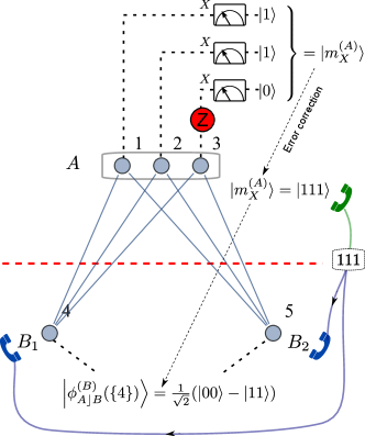
(a)

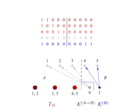
(b)

Figure 10: (Color online) An example of entanglement localization of graph states protected against errors: (a) Local X-measurements on subsystem $A$ project the graph state $\ket{G}$ onto the maximally entangled state $\ket{\phi_{A\rfloor B}^{(B)}(\xi)}$ for subsystem $B$. Under the assumption of a single qubit error, the outcome $\ket{m_{X}^{(A)}}=\ket{110}$ indicates a Z-error on vertex $3$. Alice sends Bob the corrected outcome $(111)$, such that Bob knows from the Schmidt decomposition that he possesses the state $\ket{\phi_{A\rfloor B}^{(B)}(\{4\})}$. (b) Binary representation and incidence structure after $A\rfloor B$-factorization.

In this section, we consider the localization of entanglement PoppVMCirac2005-LocalizableEnt on graph states shared between Alice and Bob ($A|B$-bipartition); see Fig. 10a. Alice measures the graph state with Pauli-measurements on her system, then tells Bob her measurement results via a classical channel. At the end, Bob should possess a bipartite maximally entangled state which he knows. A connected graph state is maximally “connected” with respect to entanglement localization, if every pair of vertices can be projected onto a Bell pair with local measurements GraphStateReviews2006 . The simplest approach to localize the entanglement of $\ket{G}$ in the subsystem $\{B_{1},B_{2}\}$ is finding a path between $B_{1}$ and $B_{2}$, then removing vertices outside the path with Z-measurements, and, at the end, measuring each vertex on the path between $\{B_{1},B_{2}\}$ in the X-direction. However, the resulting state depends on the measurement outcomes. If errors occur in Alice’s measurements, it will lead to a wrong state of Bob. Therefore, error correction would be a nice feature in the entanglement localization of graph states.

Graph states are stabilizer states. These states can be exploited as quantum stabilizer codes Gottesman1996-QECSQHB ; Gottesman1997-phdQEC ; NielsenChuang2004-QCQI ; GraphStateReviews2006 , which are linear codes and protect against errors. In the Schmidt decomposition, the measurement outcomes on the system $A$ imply which states are projected in the system $B$. The existence of X-chains on Alice’s side can provide simple repetition codes as the Schmidt basis in the Schmidt decomposition in the X-basis. Therefore, instead of removing the vertices outside a selected path between $B_{1}$ and $B_{2}$, we will make X-measurements on them to take the benefit of X-chains for the error correction.

The graph state $\ket{G}$ in Fig. 10a is taken as an example. This state has the X-chain generating set $\Gamma_{G}=\{\{1,2\},\{1,3\},\{4,5\}\}$. The generating set of the three correlation groups (Eq. (52), (53) and (54)) for the Schmidt decomposition are $\mathcal{K}_{A}^{(A)}=\mathcal{K}_{\sim B}^{(A)}=\emptyset$ and $\mathcal{K}^{(B)}=\{\{1\}\}$, while the generating set of the $(A\rightharpoonup B)$-correlation group is $\mathcal{K}^{(A\rightharpoonup B)}=\{\{4\}\}$. According to Theorem 22 and with the help of Algorithm 23, one has

$$|\psi_{A\rfloor B}(\emptyset)\rangle=\left|000\right\rangle\frac{\left|00\right\rangle+\left|11\right\rangle}{\sqrt{2}}$$ (72)

and

$$|\psi_{A\rfloor B}(\{4\})\rangle=\left|111\right\rangle\frac{\left|00\right\rangle-\left|11\right\rangle}{\sqrt{2}}.$$ (73)

As a result, the Schmidt decomposition of the graph state is

$$|G\rangle=\frac{1}{\sqrt{2}}\left(\left|000\right\rangle\frac{\left|00\right\rangle+\left|11\right\rangle}{\sqrt{2}}+\left|111\right\rangle\frac{\left|00\right\rangle-\left|11\right\rangle}{\sqrt{2}}\right).$$ (74)

In this example, one observes that there are $2$ X-chain generators $\{1,2\}$ and $\{1,3\}$ on Alice’s $3$-qubit system. This encodes the following $[3,1,3]$ repetition code Gottesman1996-QECSQHB ; Gottesman1997-phdQEC ; NielsenChuang2004-QCQI in the Schmidt vectors on Alice’s system:

$$|\phi_{A\rfloor B}^{(A)}(0)\rangle=|000\rangle\text{ and }|\phi_{A\rfloor B}^{(A)}(\{4\})\rangle=|111\rangle.$$ (75)

These codes have the Hamming distance $3$. Thus, a single Z-error can be corrected. After a measurement in the X-basis, Alice can therefore correct her result before sending it to Bob. In this approach, Bob will gain the correct acknowledgment of his maximally entangled state after Alice’s measurement with confidence. Although the repetition code cannot correct phase errors (the X-errors in X-measurements), it is already sufficient for our task, since a phase error on Alice’s side does not change the measurement outcomes.

This application may be useful for quantum repeaters BriegelDCZoller1998-QRepeater . The parties $B_{1}$ and $B_{2}$ can be at a large distance, such that they are not able to directly create an entangled state between them. In this case, they need the help from Alice as a repeater station to project the entanglement onto $B_{1}$ and $B_{2}$.

VI Conclusions

In this paper, we discussed properties of the representation of graph states in the computational X-basis. We introduced the framework of X-resources and correlation indices and linked them to the binary representation of graph states. A special type of X-resources was defined as X-chains: an X-chain is a subset of vertices for a given graph, such that the product of the stabilizer generators associated with these vertices contains only $\sigma_{X}$-Pauli operators. The set of X-chains of a graph state is a group, which can be calculated efficiently WuKampermannBruss2015-XChainAlgo . The X-chain groups revealed structures of graph states and showed how to distinguish them by local $\sigma_{X}$ measurements. We introduced X-chain factorization (Lemma 8, 13) for deriving the representation of graph states in the X-basis, and it was shown that a graph state can be represented as superposition of all X-chain states (Theorem 13). This approach was illustrated in the so-called factorization diagram (Algorithm 14). The larger the X-chain group is, the fewer X-chain states are needed for representing the graph state.

We demonstrated various applications of the X-chain factorization. An important application is its usefulness for efficiently determining the overlap of two graph states (Corollary 16) using our algorithm.

Further, we generalized the X-chain factorization approach such that it allows to find the Schmidt decomposition of graph states, which is the superposition of appropriately selected correlation states (Theorem 22, Algorithm 23 and MATHEMATICA package in the Supplemental Material XchainMpackage_Wu ).

Further benefits of the X-chain factorization are error correction procedures in entanglement localization of graph states in bipartite systems. This could be useful for quantum repeaters BriegelDCZoller1998-QRepeater .

The results of this paper can be extended to general multipartite graph states, e.g. weighted graph states DurHHLBriegel2005-EntSpinChain ; HartmannCDB2007-04 and hypergraph states RossiHBMacchiavello2013-11 ; QuWLBao2013-02 ; GuhneCSMRBKM2014 . Another possible extension of these results is to consider the representation of graph states in a hybrid basis, i.e. for a subset of the qubits one adopts the X-basis, while for the other parties one uses the Z-basis. The graph state in such a hybrid basis can even have a simpler representation (i.e. a smaller number of terms in the superposition) than the one obtained by X-chain factorization. Besides, in HeinEisertBriegel2004-06 ; GraphStateReviews2006 ; CosentinoSimone2009-Weight ; HajdusekMurao2013-Direct , various multipartite entanglement measures for graph states were studied. We expect that the approach of X-chain factorization may also be useful in these cases.

Appendix A Proofs

Proposition 2 shows the isomorphism between the stabilizer group and power set of the graph vertex set. It is proved as follows.

Proposition 2 (Isomorphism of $\xi$-induction).

Let $\left(\mathcal{S}_{G},\cdot\right)$ be the stabilizer group of a graph state $|G\rangle$ and $\mathcal{P}(V_{G})$ be the power set of the vertex set of $G$. The vertex-induction operation $s_{G}^{(\xi)}$ is a group isomorphism between $(\mathcal{P}(V_{G}),\Delta)$ and $(\mathcal{S}_{G},\cdot)$, i.e.

$$(\mathcal{P}(V_{G}),\Delta)\overset{s_{G}^{(\xi)}}{\sim}\left(\mathcal{S}_{G},\cdot\right),$$ (76)

where $\Delta$ is the symmetric difference operation.

Proof of Proposition 2.

Let $\xi_{1}$, $\xi_{2}\subseteq V_{G}$ be two vertex subsets. Since the stabilizer group $\mathcal{S}_{G}$ is Abelian, one can resort the product as $s_{G}^{(\xi_{1})}s_{G}^{(\xi_{2})}=\prod_{i\in\xi_{1}\Delta\xi_{2}}g_{i}\prod_{i^{\prime}\in\xi_{1}\cap\xi_{2}}(g_{i^{\prime}})^{2}$. The property $(g_{i})^{2}=\mathbbm{1}$ leads to $s_{G}^{(\xi_{1})}s_{G}^{(\xi_{2})}=s_{G}^{(\xi_{1}\Delta\xi_{2})}$. Therefore $s_{G}^{(\xi)}$ is a group homomorphism $(\mathcal{P}(V_{G}),\Delta)\overset{s_{G}^{(\xi)}}{\rightarrow}\left(\mathcal{S}_{G_{k}},\cdot\right)$. The kernel of $s_{G}^{(\xi)}$ is $\emptyset$, therefore $(\mathcal{P}(V_{G}),\Delta)\overset{s_{G}^{(\xi)}}{\sim}\left(\mathcal{S}_{G},\cdot\right)$. ∎

Proposition 5 provides us with a mathematical expression of $\xi$-induce graph state stabilizer. It is proven by counting of the exchanging times of Pauli $X$ and $Z$ operators.

Proposition 5 (Induced stabilizer).

Let $\xi$ be a vertex subset of a graph $G$. The $\xi$-induced stabilizer (see Def. 1) of a graph state $|G\rangle$ is given by

$$s_{G}^{(\xi)}=\pi_{G}\left(\xi\right)\sigma_{X}^{(\xi)}\sigma_{Z}^{(c_{\xi})}$$ (77)

where $c_{\xi}$ is the correlation index of $\xi$ and $\pi_{G}\left(\xi\right)$ is the stabilizer parity of $\xi$.

Proof of Proposition 5.

Let $\xi=\left\{j_{1},...,j_{m}\right\}$. Once we write down the $\xi$-induced stabilizers explicitly, we have

$$s_{G}^{\left(\xi\right)}=\sigma_{x}^{(j_{1})}\sigma_{z}^{(N_{j_{1}})}\cdots\sigma_{x}^{(j_{m})}\sigma_{z}^{(N_{j_{m}})}$$ (78)

with $N_{j}$ being the neighborhood of $j$. Now we shift $\sigma_{x}$ operators to re-sort the expression such that all the $\sigma_{x}$ are on the left side of $\sigma_{z}$. First, let us consider the last $X$-operator, $\sigma_{x}^{(j_{m})}$. The number of $\sigma_{z}^{(j_{m})}$ on the left hand side of $\sigma_{x}^{(j_{m})}$ indicates how many times one needs to exchange $\sigma_{x}^{(j_{m})}$ and $\sigma_{z}^{(j_{m})}$. It is equal to the number of neighbors of $j_{m}$ in the $\xi$-induced graph $G[\xi]$, namely $d_{j_{m}}(G[\xi])$. Due to the anti-commutativity of $\sigma_{x}$ and $\sigma_{z}$, the shifting brings us a prefactor $(-1)^{d_{j_{m}}(G\left[\xi\right])}$. Recursively, shifting $\sigma_{x}^{(j_{m}-1)}$ to the left side of $\sigma_{z}^{(j_{m}-1)}$ brings us a prefactor $(-1)^{d_{j_{k-1}}(G\left[\xi\right]-j_{m})}$, and so on. In total, the times that one needs to exchange $\sigma_{x}$ and $\sigma_{z}$ is

$$d_{j_{k}}(G\left[\xi\right])+d_{j_{k-1}}(G\left[\xi\right]-j_{m})+\cdots+d_{2}(G\left[\left\{j_{1},j_{2}\right\}\right]),$$ (79)

which is equal to the edge number $\left|E(G[\xi])\right|$. Hence, after the shifting, we obtain a product of re-sorted $\sigma_{x}$ and $\sigma_{z}$ operators with a prefactor $(-1)^{\left|E(G[\xi])\right|}$, i.e.,

$$s_{G}^{(\xi)}=(-1)^{\left|E(G[\xi])\right|}\sigma_{x}^{(j)}\sigma_{z}^{(n_{G}\left(j_{1}\right))}\cdots\sigma_{z}^{(n_{G}\left(j_{m}\right))},$$ (80)

while $\sigma_{z}^{(N(j_{1}))}\cdots\sigma_{z}^{(N(j_{m}))}=\sigma_{z}^{c_{G}(\xi)}$. ∎

Lemma 8 regroups the power set of vertices with factorization regarding the X-chain group into the correlation group. Accordingly, one can regroup the graph state projector by stabilizers induced by the correlation group. It is a result of Proposition 2.

Lemma 8 (X-chain groups and correlation groups).

Let $|G\rangle$ be a graph state. The set of X-chains together with the symmetric difference $(\mathcal{X}_{G}^{\left(\emptyset\right)},\Delta)$, is a normal subgroup of $\left(\mathcal{P}\left(V_{G}\right),\Delta\right)$. The quotient group $(\mathcal{P}\left(V_{G}\right)/\mathcal{X}_{G}^{\left(\emptyset\right)},\Delta)$ is identical to the set of all resource sets

$$\mathcal{P}\left(V_{G}\right)/\mathcal{X}_{G}^{\left(\emptyset\right)}=\left\{\mathcal{X}_{G}^{\left(c\right)}:c\in\mathcal{C}_{G}\right\},$$ (81)

which we call call the correlation group of $\ket{G}$. Let $\Gamma_{G}$ and $\mathcal{K}_{G}$ denote the generating sets of $(\mathcal{X}_{G}^{\left(\emptyset\right)},\Delta)$ and $(\mathcal{P}(V_{G})/\mathcal{X}_{G}^{(\emptyset)},\Delta)$, respectively. The stabilizer group $\left(\mathcal{S}_{G},\cdot\right)$ is isomorphic to the direct product of the X-chain group and the correlation group,

$$\left(\mathcal{S}_{G},\cdot\right)\sim\left(\left\langle\Gamma_{G}\right\rangle,\Delta\right)\times\left(\left\langle\mathcal{K}_{G}\right\rangle,\Delta\right),$$ (82)

As a result, the graph state $|G\rangle$ is the product of the X-chain group and correlation group inducing stabilizers, i.e.

$$|G\rangle\langle G|=\prod_{\kappa\in\mathcal{K}_{G}}\frac{1+s_{G}^{(\kappa)}}{2}\prod_{\gamma\in\Gamma_{G}}\frac{1+s_{G}^{(\gamma)}}{2}.$$ (83)

Proof of Lemma 8.

Let $\xi_{1}$ and $\xi_{2}$ be two elements of $\mathcal{X}_{G}^{\left(c\right)}$. The correlation index mapping, $c_{G}:\left(\mathcal{P}(V_{G}),\Delta\right)\rightarrow\left(\mathcal{C}_{G},\Delta\right)$, is a group homomorphism, since $c_{G}\left(\xi_{1}\Delta\xi_{2}\right)=c_{G}\left(\xi_{1}\right)\Delta c_{G}\left(\xi_{2}\right)$. Due to the definition of X-chains that $c_{G}(\xi)=0$, $(\mathcal{X}_{G}^{\left(\emptyset\right)},\Delta)$ is the kernel of the mapping $c_{G}$. Since $\left(\mathcal{P}\left(V_{G}\right),\Delta\right)$ is Abelian, the kernel $(\mathcal{X}_{G}^{\left(\emptyset\right)},\Delta)$ and the correlation group $\mathcal{P}\left(V_{G}\right)/\mathcal{X}_{G}^{\left(\emptyset\right)}$ are both normal subgroups. The correlation group $\braket{\mathcal{K}_{G}}$ is obtained via

$$\braket{\mathcal{K}_{G}} =\mathcal{P}\left(V_{G}\right)/\mathcal{X}_{G}^{\left(\emptyset\right)}$$

$$=\left\{\xi\Delta\mathcal{X}_{G}^{\left(\emptyset\right)}:\xi\in\mathcal{P}\left(V_{G}\right)\right\}$$

$$=\left\{\mathcal{X}_{G}^{\left(c\right)}:c\in\mathcal{C}_{G}\right\}.$$ (84)

As a result of group theory,

$$\left(\mathcal{P}(V_{G}),\Delta\right)=\left(\left\langle\Gamma_{G}\right\rangle,\Delta\right)\times\left(\left\langle\mathcal{K}_{G}\right\rangle,\Delta\right).$$ (85)

According to Proposition 2, one obtains the isomorphism

$$\left(\mathcal{S}_{G_{k}},\cdot\right)\overset{s_{G_{k}}^{(\xi)}}{\sim}\left(\left\langle\Gamma_{G}\right\rangle,\Delta\right)\times\left(\left\langle\mathcal{K}_{G}\right\rangle,\Delta\right).$$ (86)

The projector of graph state $|G\rangle\langle G|$ is the sum of all $\xi$-induced stabilizers, $s_{G}^{(\xi)}$, with $\xi\in\left\langle\Gamma_{G}\right\rangle\times\left\langle\mathcal{K}_{G}\right\rangle$. As a result,

$$|G\rangle\langle G| =\sum_{\xi\in\mathcal{P}\left(V_{G}\right)}s_{G}^{(\xi)}$$

$$=\prod_{\kappa\in\mathcal{K}_{G}}\frac{1+s_{G}^{(\kappa)}}{2}\prod_{\gamma\in\mathcal{\Gamma}_{G}}\frac{1+s_{G}^{(\gamma)}}{2}.$$ (87)

∎

Proposition 10 (X-chain states in X-basis).

Let $|G\rangle$ be a graph state with the X-chain group $\left\langle\Gamma_{G}\right\rangle$ and the correlation group $\left\langle\mathcal{K}_{G}\right\rangle$. Let $\Gamma_{G}=\left\{\gamma_{1},\gamma_{2},...\right\}$, and $\gamma_{i}=\left\{v_{i_{1}},v_{i_{2}},\cdots\right\}$. The generating set $\Gamma_{G}$ and $\mathcal{K}_{G}$ can be chosen as

1. $\Gamma_{G}=\{\gamma_{1},...,\gamma_{k}\}$ such that $\gamma_{i}\not\subseteq\gamma_{j}$ for all $\gamma_{i},\gamma_{j}\in\Gamma_{G}$,

2. $\mathcal{K}_{G}=\left\{\left\{v\right\}:v\in V_{G}\backslash\bigcup_{i=1}^{k}\left\{v_{i_{1}}\right\}\right\}$.

Here, the first element of $\gamma_{i}=\{v_{i_{1}},v_{i_{2}},...\}$ is selected in a way such that $v_{i_{1}}\neq v_{j_{1}}$ for all $i\not=j$. Then the X-chain state $\ket{\psi_{\emptyset}(\emptyset)}$ of $|G\rangle$ is an X-basis state, $|i^{(x_{\Gamma})}\rangle$, with

$$x_{\Gamma}=\left\{v_{i_{1}}:\pi_{G}\left(\gamma_{i}\right)=-1\right\}.$$ (88)

Proof of Proposition 10.

Let $\gamma_{i}^{-}$ be an X-chain generator with negative parity $\pi_{G}\left(\gamma_{i}^{-}\right)=-1$, then $v_{i_{1}}\in x_{\Gamma}$. Since $v_{i_{1}}\in\gamma_{i}$ and $v_{i_{1}}\not\in\gamma_{j}$ for all $j\not=i$, the intersection $\gamma_{i}^{-}\cap x_{\Gamma}=\left\{v_{i_{1}}\right\}$, hence $\pi_{G}\left(\gamma_{i}^{-}\right)\sigma_{x}^{(\gamma_{i})}|i^{(x_{\Gamma})}\rangle=|i^{(x_{\Gamma})}\rangle$. For an X-chain generator $\gamma_{j}^{+}$ with positive parity $\pi_{G}\left(\gamma_{i}^{+}\right)=1$, the intersection $\gamma_{i}^{+}\cap x_{\Gamma}=\emptyset$, and therefore $\pi_{G}\left(\gamma_{i}^{+}\right)\sigma_{x}^{(\gamma_{i})}|i^{(x_{\Gamma})}\rangle=|i^{(x_{\Gamma})}\rangle$. Hence the condition 1 in Definition 9 is fulfilled.

Let $\left\{v\right\}\in\mathcal{K}_{G}$ be a generator of correlation group, then $\sigma_{x}^{(\{v\})}|i^{(x_{\Gamma})}\rangle=\left(-1\right)^{\left|x_{\Gamma}\cap\left\{v\right\}\right|}|i^{(x_{\Gamma})}\rangle=|i^{(x_{\Gamma})}\rangle$, since $\left|x_{\Gamma}\cap\left\{v\right\}\right|=0$ according to the choice of $\mathcal{K}_{G}$. Hence, the condition 2 in Definition 9 is fulfilled. ∎

The Proposition 11 derives the correlation states as the summation of X-chain states. It follows directly from their definition.

Proposition 11 (Form of X-chain states, $\mathcal{K}$-correlation states).

Let $\xi\in\left\langle\mathcal{K}_{G}\right\rangle$ be an X-resource and $\left\langle\mathcal{K}\right\rangle\subseteq\left\langle\mathcal{K}_{G}\right\rangle$. An X-chain state is given as

$$|\psi_{\emptyset}\left(\xi\right)\rangle=\pi_{G}\left(\xi\right)\left|i^{(x_{\Gamma})}\oplus i^{(c_{\xi})}\right\rangle,$$ (89)

where $\pi_{G}\left(\xi\right)$ is the stabilizer parity of $\xi$ (see Eq. (13)), and $c_{\xi}$ is the correlation index of $\xi$.

A $\mathcal{K}$-correlation state is the superposition of X-chain states,

$$|\psi_{\mathcal{K}}\left(\xi\right)\rangle=\frac{1}{2^{\left|\mathcal{K}\right|/2}}\sum_{\xi^{\prime}\in\left\langle\mathcal{K}\right\rangle}|\psi_{\emptyset}\left(\xi\Delta\xi^{\prime}\right)\rangle.$$ (90)

Proof of Proposition 11.

According to Proposition 2, $s_{G}^{(\xi)}\Delta s_{G}^{(\xi^{\prime})}=s_{G}^{(\xi\Delta\xi^{\prime})}$, the product of the operators in Eq. (25) can be reformulated to the sum of

$$|\psi_{\mathcal{K}}\left(\xi\right)\rangle=\frac{1}{2^{\left|\mathcal{K}\right|/2}}\sum_{\xi^{\prime}\in\left\langle\mathcal{K}\right\rangle}s_{G}^{(\xi\Delta\xi^{\prime})}\left|i^{(x_{\Gamma})}\right\rangle.$$ (91)

With the formulas in Proposition 5,

$$|\psi_{\mathcal{K}}\left(\xi\right)\rangle=\frac{1}{2^{\left|\mathcal{K}\right|/2}}\sum_{\xi^{\prime}\in\left\langle\mathcal{K}\right\rangle}\pi_{G}\left(\xi\Delta\xi^{\prime}\right)\sigma_{z}^{(c_{\xi\Delta\xi^{\prime}})}\sigma_{x}^{(\xi\Delta\xi^{\prime})}\left|i^{(x_{\Gamma})}\right\rangle.$$ (92)

Since $\sigma_{x}^{(\kappa)}\left|i^{(x_{\Gamma})}\right\rangle=\left|i^{(x_{\Gamma})}\right\rangle$ for all $\kappa\in\left\langle\mathcal{K}\right\rangle$, one obtains

$$|\psi_{\mathcal{K}}\left(\xi\right)\rangle=\frac{1}{2^{\left|\mathcal{K}\right|/2}}\sum_{\xi^{\prime}\in\left\langle\mathcal{K}\right\rangle}\pi_{G}\left(\xi\Delta\xi^{\prime}\right)\left|i^{(x_{\Gamma})}\oplus i^{(c_{\xi\Delta\xi^{\prime}})}\right\rangle.$$ (93)

∎

The following calculation is the proof of Corollary 12, which is employed in the proof of Theorem 13.

Proof of Corollary 12.

The properties (2) and (3) are direct results of Proposition 11. Property (1) follows from the commutativity of graph state stabilizers. Let $\kappa=\gamma\Delta\kappa_{0}\in\left\langle\Gamma_{G}\right\rangle\times\left\langle\mathcal{K}\right\rangle$ with $\gamma\in\left\langle\Gamma_{G}\right\rangle$ and $\kappa_{0}\in\left\langle\mathcal{K}\right\rangle$; then

$$s_{G}^{(\kappa)}\phi_{\mathcal{K}}\left(\xi\right) =s_{G}^{(\gamma)}s_{G}^{(\kappa_{0})}s_{G}^{(\xi)}\prod_{\kappa^{\prime}\in\mathcal{K}}\frac{1+s_{G}^{(\kappa^{\prime})}}{\sqrt{2}}|x_{\Gamma}\rangle$$

$$=s_{G}^{(\xi)}\frac{1}{2^{\left|\mathcal{K}\right|/2}}s_{G}^{(\kappa_{0})}\sum_{\kappa^{\prime}\in\left\langle\mathcal{K}\right\rangle}s_{G}^{(\kappa^{\prime})}s_{G}^{(\gamma)}|x_{\Gamma}\rangle.$$

Due to the definition of $|x_{\Gamma}\rangle$, it holds that $s_{G}^{(\gamma)}|x_{\Gamma}\rangle=|x_{\Gamma}\rangle$. Since $\kappa_{0}\in\left\langle\mathcal{K}\right\rangle$, the operator $s_{G}^{(\kappa_{0})}\sum_{\kappa^{\prime}\in\left\langle\mathcal{K}\right\rangle}s_{G}^{(\kappa^{\prime})}=\sum_{\kappa^{\prime}\in\left\langle\mathcal{K}\right\rangle}s_{G}^{(\kappa^{\prime})}$ is not changed by $s_{G}^{(\kappa_{0})}$, hence

$$s_{G}^{(\kappa)}\ket{\phi_{\mathcal{K}}\left(\xi\right)}=s_{G}^{(\xi)}\frac{1}{2^{\left|\mathcal{K}\right|/2}}\sum_{\kappa^{\prime}\in\left\langle\mathcal{K}\right\rangle}s_{G}^{(\kappa^{\prime})}|x_{\Gamma}\rangle=\ket{\phi_{\mathcal{K}}\left(\xi\right)}.$$ (94)

∎

Lemma 20 shows us the $A|B$-separability of the correlation state $|\psi_{A\rfloor B}(\xi)\rangle$. It is a result of the property of multiplication $G$-parities.

Lemma 24 (Multiplication of $G$-parity).

Let $G$ be a graph; then the multiplication of two of the parities of two-vertex subset $\pi_{G}\left(\xi_{1}\right)$ and $\pi_{G}\left(\xi_{2}\right)$ is equal to

$$\pi_{G}\left(\xi_{1}\right)\pi_{G}\left(\xi_{2}\right)=\left(-1\right)^{\left|E_{G}(\xi_{1}:\xi_{2})\right|}\pi_{G}\left(\xi_{1}\Delta\xi_{2}\right).$$ (95)

Proof.

Since $\left(P(V),\Delta\right)$ is isomorphic to the stabilizer group $\left(S_{G},\cdot\right)$, it holds then that

$$s_{G}^{(\xi_{1})}s_{G}^{(\xi_{2})}=s_{G_{k}}^{(\xi_{1}\Delta\xi_{2})}.$$

Reorder the $\sigma_{x}$ and $\sigma_{z}$ in both sides, such that $\sigma_{x}$ are on the left side of $\sigma_{z}$; then one obtains

$$\pi_{G}\left(\xi_{1}\right)\pi_{G}\left(\xi_{2}\right)=\left(-1\right)^{\left|E_{G}(\xi_{1}:\xi_{2})\right|}\pi_{G}\left(\xi_{1}\Delta\xi_{2}\right).$$ (96)

∎

With this lemma one can prove Lemma 20 as follows.

Lemma 20 ($A|B$-Separability of $A\rfloor B$-correlation states).

For $\xi\in\langle\mathcal{K}_{G}^{A\rightharpoonup B}\rangle$, the $\left(A\rightharpoonup B\right)$-correlation states

$$|\psi_{A\rfloor B}(\xi)\rangle=\pi_{G}\left(\xi\right)|\phi_{A\rfloor B}^{(A)}(\xi)\rangle|\phi_{A\rfloor B}^{(B)}(\xi)\rangle$$ (97)

are $A|B$-separable with $|\phi_{A\rfloor B}^{(A)}(\xi)\rangle:=|\psi_{\mathcal{K}_{A}^{(A)}\cup\mathcal{K}_{\sim B}^{(A)}}^{(A)}(\xi)\rangle$ and $|\phi_{A\rfloor B}^{(B)}(\xi)\rangle:=|\psi_{\mathcal{K}^{(B)}}^{(B)}(\xi)\rangle$ being the $(\mathcal{K}_{A}^{(A)}\cup\mathcal{K}_{\sim B}^{(A)})$- and $\mathcal{K}^{(B)}$-correlation states projected into the subspaces of $A$ and $B$, respectively.

Proof of Lemma 20.

According to Proposition 11,

$$|\psi_{A\rfloor B}(\xi)\rangle=\sum_{\xi^{\prime}\in\left\langle\mathcal{K}_{A}^{(A)}\cup\mathcal{K}_{\sim B}^{(A)}\cup\mathcal{K}^{(B)}\right\rangle}\pi_{G}\left(\xi^{\prime}\Delta\xi\right)|x_{\Gamma}\oplus c_{\xi^{\prime}}\oplus c_{\xi}\rangle.$$ (98)

Each X-resource $\xi^{\prime}\in\left\langle\mathcal{K}_{A}^{(A)}\cup\mathcal{K}_{\sim B}^{(A)}\cup\mathcal{K}^{(B)}\right\rangle$ can be decomposed as $\xi^{\prime}=\alpha\Delta\beta=\alpha_{A}\Delta\alpha_{B}\Delta\beta$ with $\alpha_{A}\in\left\langle\mathcal{K}_{A}^{(A)}\right\rangle$ and $\alpha_{B}\in\left\langle\mathcal{K}_{\sim B}^{(A)}\right\rangle$ and $\beta\in\left\langle\mathcal{K}^{(B)}\right\rangle$. Due to Lemma 24

$$\pi_{G}\left(\xi^{\prime}\Delta\xi\right)=\left(-1\right)^{\left|E_{G}(\xi:\alpha\Delta\beta)\right|}\pi_{G}\left(\alpha\Delta\beta\right)\pi_{G}\left(\xi\right)\text{ and }\pi_{G}\left(\alpha\Delta\beta\right)=\left(-1\right)^{\left|E_{G}(\alpha:\beta)\right|}\pi_{G}\left(\alpha\right)\pi_{G}\left(\beta\right)$$ (99)

Since $\alpha_{A}\subseteq A$ and $c_{\beta}\subseteq B$, it holds $\left|E_{G}(\alpha_{A}:\beta)\right|\overset{\operatorname{mod}2}{=}\left|\alpha_{A}\cap c_{\beta}\right|\overset{\operatorname{mod}2}{=}0$, while $\alpha_{B}\in\left\langle\mathcal{K}_{\sim B}^{(A)}\right\rangle$ is defined by $\left|E_{G}(\alpha_{B}:\beta)\right|\overset{\operatorname{mod}2}{=}$ $0$. Therefore the edge number is $\left|E_{G}(\alpha:\beta)\right|=\left|E_{G}(\alpha_{A}\Delta\alpha_{B}:\beta)\right|\overset{\operatorname{mod}2}{=}0$. In addition, $\left|E_{G}(\xi:\alpha\Delta\beta)\right|\overset{\operatorname{mod}2}{=}\left|E_{G}(\xi:\alpha)\right|+\left|E_{G}(\xi:\beta)\right|$, and therefore

$$\pi_{G}\left(\xi^{\prime}\Delta\xi\right)=\left(-1\right)^{\left|E_{G}(\xi:\alpha)\right|}\left(-1\right)^{\left|E_{G}(\xi:\beta)\right|}\pi_{G}\left(\alpha\right)\pi_{G}\left(\beta\right)\pi_{G}\left(\xi\right)$$

According to Eq. (13) in Proposition 5, the following equation holds

$$\pi_{G}\left(\xi\right)\left(-1\right)^{\left|E_{G}(\xi:\beta)\right|}\pi_{G}\left(\beta\right)=\left(-1\right)^{\left|E(G\left[\beta\right])\right|+\left|E_{G}(\xi:\beta)\right|+\left|E(G\left[\xi\right])\right|}=\left(-1\right)^{\left|E(G\left[\beta\Delta\xi\right])\right|}=\pi_{G}\left(\xi\Delta\beta\right).$$ (100)

This equality also holds for $\alpha$, and therefore

$$\pi_{G}\left(\xi^{\prime}\Delta\xi\right)=\pi_{G}\left(\alpha\Delta\xi\right)\pi_{G}\left(\beta\Delta\xi\right)\pi_{G}\left(\xi\right).$$ (101)

Insert this equality into Eq. (33), and one obtains

$$|\psi_{A\rfloor B}(\xi)\rangle=\pi_{G}\left(\xi\right)\sum_{\alpha\in\left\langle\mathcal{K}_{A}^{(A)}\right\rangle}\sum_{\beta\in\left\langle\mathcal{K}^{(B)}\right\rangle}\pi_{G}\left(\alpha\Delta\xi\right)\pi_{G}\left(\beta\Delta\xi\right)|i^{(x_{\Gamma})}\oplus i^{(c_{\alpha})}\oplus i^{(c_{\beta})}\oplus i^{(c_{\xi})}\rangle=\pi_{G}\left(\xi\right)|\phi_{A\rfloor B}^{(A)}(\xi)\rangle|\phi_{A\rfloor B}^{(B)}(\xi)\rangle$$ (102)

with

$$|\phi_{A\rfloor B}^{(A)}(\xi)\rangle=|\psi_{\mathcal{K}_{A}^{(A)}\cup\mathcal{K}_{\sim B}^{(A)}}^{(A)}(\xi)\rangle=\sum_{\alpha\in\left\langle\mathcal{K}_{A}^{(A)}\cup\mathcal{K}_{\sim B}^{(A)}\right\rangle}\pi_{G}\left(\alpha\Delta\xi\right)|i^{(x_{\Gamma}^{(A)})}\oplus i^{(c_{\alpha})}\oplus i^{(c_{\xi}^{(A)})}\rangle,$$ (103)

and

$$|\phi_{A\rfloor B}^{(B)}(\xi)\rangle=|\psi_{\mathcal{K}^{(B)}}^{(B)}(\xi)\rangle=\sum_{\beta\in\left\langle\mathcal{K}^{(B)}\right\rangle}\pi_{G}\left(\beta\Delta\xi\right)|i^{(x_{\Gamma}^{(B)})}\oplus i^{(c_{\beta})}\oplus i^{(c_{\xi}^{(B)})}\rangle.$$ (104)

∎

Lemma 21 is the key to derive Theorem 22. Its proof is as follows.

Lemma 21 (Orthonormality of $(A\rightharpoonup B)$-correlation states).

The components of $A\rfloor B$-correlation states on subspace $A$ and $B$, $|\phi_{A\rfloor B}^{(A)}(\xi)\rangle$ and $|\phi_{A\rfloor B}^{(B)}(\xi)\rangle$, are orthonormal with respect to $\xi\in\langle\mathcal{K}^{A\rightharpoonup B}\rangle$ within the subspaces $A$ and $B$, respectively, i.e.,

$$\langle\phi_{A\rfloor B}^{(A)}(\xi_{1})|\phi_{A\rfloor B}^{(A)}(\xi_{2})\rangle=0$$ (105)

and

$$\langle\phi_{A\rfloor B}^{(B)}(\xi_{1})|\phi_{A\rfloor B}^{(B)}(\xi_{2})\rangle=0$$

for all $\xi_{1},\xi_{2}\in\langle\mathcal{K}^{A\rightharpoonup B}\rangle$ and $\xi_{1}\not=\xi_{2}$.

Proof of Lemma 21.

According to the definition of correlation states (Def. 9) and the unitarity of stabilizer $s_{G}^{(\xi_{1})}$ and $s_{G}^{(\xi_{2})}$, it holds that

$$\langle\phi_{\mathcal{K}}(\xi_{1})|\phi_{\mathcal{K}}(\xi_{2})\rangle=\langle\phi_{\mathcal{K}}(0)|\phi_{\mathcal{K}}(\xi_{1}\Delta\xi_{2})\rangle.$$ (106)

One just needs to consider the overlap $\langle\phi_{A\rfloor B}^{(A)}(0)|\phi_{A\rfloor B}^{(A)}(\xi)\rangle$ and $\langle\phi_{A\rfloor B}^{(B)}(0)|\phi_{A\rfloor B}^{(B)}(\xi)\rangle$ with $\xi\in\langle\mathcal{K}_{G}^{A\rightharpoonup B}\rangle$. That means for all $\alpha\in\langle\mathcal{K}_{A}^{(A)}\cup\mathcal{K}_{\sim B}^{(A)}\rangle$ and $\beta\in\langle\mathcal{K}^{(B)}\rangle$, it holds that

$$c_{\alpha}\oplus c_{\beta}\not=c_{\xi}.$$ (107)

For $|\phi_{A\rfloor B}^{(A)}(\xi)\rangle$, due to the commutativity of graph state stabilizers, it holds that

$$\langle\phi_{A\rfloor B}^{(A)}(0)|\phi_{A\rfloor B}^{(A)}(\xi)\rangle =\frac{1}{2^{\left|\mathcal{K}_{A}^{(A)}\cup\mathcal{K}_{\sim B}^{(A)}\right|}}\sum_{\alpha,\alpha^{\prime}\in\left\langle\mathcal{K}_{A}^{(A)}\cup\mathcal{K}_{\sim B}^{(A)}\right\rangle}\pi_{G}\left(\alpha^{\prime}\right)\pi_{G}\left(\alpha\Delta\xi\right)\langle i(x_{\Gamma}^{(A)})\oplus i(c_{\alpha^{\prime}})|i(x_{\Gamma}^{(A)})\oplus i(c_{\alpha})\oplus i(c_{\xi}^{(A)})\rangle$$ (108)

$$=\frac{1}{2^{\left|\mathcal{K}_{A}^{(A)}\cup\mathcal{K}_{\sim B}^{(A)}\right|}}\sum_{\alpha,\alpha^{\prime}\in\left\langle\mathcal{K}_{A}^{(A)}\cup\mathcal{K}_{\sim B}^{(A)}\right\rangle:c_{\alpha\Delta\alpha^{\prime}}=c_{\xi}^{(A)}}\pi_{G}\left(\alpha^{\prime}\right)\pi_{G}\left(\alpha\Delta\xi\right).$$ (109)

If there exists $\lambda\in\left\langle\mathcal{K}_{A}^{(A)}\cup\mathcal{K}_{\sim B}^{(A)}\right\rangle$ such that $c_{\lambda}=c_{\xi}^{(A)}$, then $\xi\Delta\lambda\in\mathcal{K}^{(B)}$ (since $c_{\xi\Delta\lambda}\subseteq B$). This means $\xi\in\left\langle\mathcal{K}_{A}^{(A)}\cup\mathcal{K}_{\sim B}^{(A)}\right\rangle\times\left\langle\mathcal{K}^{(B)}\right\rangle$, which is in contradiction to the definition of $\xi\in\langle\mathcal{K}^{A\rightharpoonup B}\rangle$. Hence there are no pairs $\alpha,\alpha^{\prime}\in\mathcal{K}_{A}^{(A)}$ such that $c_{\alpha\Delta\alpha^{\prime}}=c_{\xi}^{(A)}$, and therefore

$$\langle\phi_{A\rfloor B}^{(A)}(0)|\phi_{A\rfloor B}^{(A)}(\xi)\rangle=0.$$ (110)

Analogously for $|\phi_{A\rfloor B}^{(B)}(\xi)\rangle$, it holds that

$$\langle\phi_{A\rfloor B}^{(B)}(0)|\phi_{A\rfloor B}^{(B)}(\xi)\rangle=\frac{1}{2^{\left|\mathcal{K}^{(B)}\right|}}\sum_{\beta,\beta^{\prime}\in\left\langle\mathcal{K}^{(B)}\right\rangle:c_{\beta\Delta\beta^{\prime}}=c_{\xi}^{(B)}}\pi_{G}\left(\beta^{\prime}\right)\pi_{G}\left(\beta\Delta\xi\right).$$ (111)

If there exists no $\lambda\in\mathcal{K}^{(B)}$ such that $c_{\lambda}=c_{\xi}^{(B)}$, then $\langle\phi_{A\rfloor B}^{(B)}(0)|\phi_{A\rfloor B}^{(B)}(\xi)\rangle=0$. If there exist such $\lambda\in\mathcal{K}^{(B)}$ then we substitute $\xi$ by $\xi^{\prime}:=\xi\Delta\lambda$, and then $\xi^{\prime}\in\left\langle\mathcal{K}^{A\rightharpoonup B}\right\rangle$ still holds and $c_{\xi^{\prime}}^{(B)}=0$. Hence the overlap becomes

$$\langle\phi_{A\rfloor B}^{(B)}(0)|\phi_{A\rfloor B}^{(B)}(\xi)\rangle =\frac{1}{2^{\left|\mathcal{K}^{(B)}\right|}}\sum_{\beta\in\left\langle\mathcal{K}^{(B)}\right\rangle}\pi_{G}\left(\beta\right)\pi_{G}\left(\beta\Delta\xi^{\prime}\right)=\frac{1}{2^{\left|\mathcal{K}^{(B)}\right|}}\sum_{\beta\in\left\langle\mathcal{K}^{(B)}\right\rangle}\left(-1\right)^{\left|E_{G}\left(\beta:\xi^{\prime}\right)\right|}$$

$$=\frac{1}{2^{\left|\mathcal{K}^{(B)}\right|}}\prod_{\beta\in\mathcal{K}^{(B)}}\left(1+\left(-1\right)^{\left|E_{G}\left(\beta:\xi^{\prime}\right)\right|}\right).$$ (112)

Since $\xi^{\prime}\in\left\langle\mathcal{K}^{A\rightharpoonup B}\right\rangle$ and $\tilde{c}_{\xi^{\prime}}\subseteq A$ implies that $\xi^{\prime}\not\subseteq A$, under the assumption that $\left|E_{G}\left(\beta:\xi^{\prime}\right)\right|\overset{\operatorname{mod}2}{=}0$ for all $\beta\in\mathcal{K}^{(B)}$, one can infer (according to the definition in Eq. (54) ) that $\xi^{\prime}\in\langle\mathcal{K}_{\sim B}^{(A)}\rangle$. This is in contradiction to the condition that $\xi^{\prime}\in\left\langle\mathcal{K}^{A\rightharpoonup B}\right\rangle$. Therefore, there must be at least one $\beta_{0}$, which has odd number of edges to $\xi^{\prime}$, i.e., $\left|E_{G}\left(\beta:\xi^{\prime}\right)\right|\overset{\operatorname{mod}2}{=}1$. Hence,

$$\langle\phi_{A\rfloor B}^{(B)}(0)|\phi_{A\rfloor B}^{(B)}(\xi)\rangle=0.$$ (113)

∎

Appendix B The list of notations

Here we present a list of symbols together with the page number where they occur for the first time.

References

- (1) H. J. Briegel and R. Raussendorf. Persistent entanglement in arrays of interacting particles. Phys. Rev. Lett., 86:910–913, 2001.
- (2) R. Raussendorf and H. J. Briegel. A one-way quantum computer. Phys. Rev. Lett., 86:5188–5191, 2001.
- (3) R. Raussendorf and H. J. Briegel. Computational model underlying the one-way quantum computer. Quant. Inf. Comp., 2:443, 2002.
- (4) R. Raussendorf, D. E. Browne, and H. J. Briegel. Measurement-based quantum computation on cluster states. Phys. Rev. A, 68:022312, 2003.
- (5) R. Raussendorf. Measurement-based quantum computation with cluster states. PhD thesis, LMU München, Germany, 2003.
- (6) M. Hein, J. Eisert, and H. J. Briegel. Multiparty entanglement in graph states. Phys. Rev. A, 69:062311, 2004.
- (7) M. Hein, W. Dür, J. Eisert, R. Raussendorf, M. V. den Nest, and H.-J. Briegel. Entanglement in graph states and its applications. arXiv:quant-ph/0602096v1, 2006.
- (8) J.-Y. Wu, H. Kampermann, and D. Bruß. Determining X-chains in graph states. arXiv:1507.06082, 2015.
- (9) See supplemental material at http://link.aps.org/supplemental/10.1103/physreva.92.012322 for the MATHEMATICA package of X-chain factorization.
- (10) M. Popp, F. Verstraete, M. A. Martín-Delgado, and J. I. Cirac. Localizable entanglement. Phys. Rev. A, 71:042306, 2005.
- (11) R. Diestel. Graph theory, volume 173 of Graduate Texts in Mathematics. Springer-Verlag, Heidelberg, 2005 edition, 2005.
- (12) M. Van den Nest. Local Equivalence of Stabilizer states and codes. PhD thesis, Katholieke Universiteit Leuven, 2005.
- (13) K. H. Rosen. Handbook of discrete and combinatorial mathematics. CRC press, 1999.
- (14) D. Gottesman. Stabilizer Codes and Quantum Error Correction. PhD thesis, 1997.
- (15) D. Gottesman. Class of quantum error-correcting codes saturating the quantum Hamming bound. Phys. Rev. A, 54:1862–1868, 1996.
- (16) A. Calderbank, E. Rains, P. Shor, and N. Sloane. Quantum error correction and orthogonal geometry. Phys. Rev. Lett., 78:405–408, 1997.
- (17) J.-Y. Wu, M. Rossi, H. Kampermann, S. Severini, L. C. Kwek, C. Macchiavello, and D. Bruß. Randomized graph states and their entanglement properties. Phys. Rev. A, 89:052335, 2014.
- (18) A. Acín, D. Bruß, M. Lewenstein, and A. Sanpera. Classification of mixed three-qubit states. Phys. Rev. Lett., 87:040401, 2001.
- (19) O. Gühne, P. Hyllus, D. Bruß, A. Ekert, M. Lewenstein, C. Macchiavello, and A. Sanpera. Detection of entanglement with few local measurements. Phys. Rev. A, 66:062305, 2002.
- (20) A. Cosentino and S. Severini. Weight of quadratic forms and graph states. Phys. Rev. A, 80:052309, 2009.
- (21) A. Shimony. Degree of entanglementa. Annals of the New York Academy of Sciences, 755(1):675–679, 1995.
- (22) H. Barnum and N. Linden. Monotones and invariants for multi-particle quantum states. Journal of Physics A: Mathematical and General, 34(35):6787, 2001.
- (23) M. Hajdušek and M. Murao. Direct evaluation of pure graph state entanglement. New Journal of Physics, 15(1):013039, 2013.
- (24) M. A. Nielsen and I. L. Chuang. Quantum Computation and Quantum Information (Cambridge Series on Information and the Natural Sciences). Cambridge University Press, 1 edition, 2004.
- (25) H.-J. Briegel, W. Dür, J. I. Cirac, and P. Zoller. Quantum repeaters: The role of imperfect local operations in quantum communication. Phys. Rev. Lett., 81:5932–5935, 1998.
- (26) W. Dür, L. Hartmann, M. Hein, M. Lewenstein, and H.-J. Briegel. Entanglement in spin chains and lattices with long-range ising-type interactions. Phys. Rev. Lett., 94:097203, 2005.
- (27) L. Hartmann, J. Calsamiglia, W. Dür, and H. J. Briegel. Weighted graph states and applications to spin chains, lattices and gases. Journal of Physics B: Atomic, Molecular and Optical Physics, 40(9):S1, 2007.
- (28) M. Rossi, M. Huber, D. Bruß, and C. Macchiavello. Quantum hypergraph states. New Journal of Physics, 15(11):113022, 2013.
- (29) R. Qu, J. Wang, Z.-S. Li, and Y.-R. Bao. Encoding hypergraphs into quantum states. Phys. Rev. A, 87:022311, 2013.
- (30) O. Gühne, M. Cuquet, F. E. S. Steinhoff, T. Moroder, M. Rossi, D. Bruß, B. Kraus, and C. Macchiavello. Entanglement and nonclassical properties of hypergraph states. Journal of Physics A: Mathematical and Theoretical, 47(33):335303, 2014.