Magnetic Energy Dissipation during the 2014 March 29 Solar Flare

Abstract

We calculated the time evolution of the free magnetic energy during the 2014-Mar-29 flare (SOL2014-03-29T17:48), the first X-class flare detected by IRIS. The free energy was calculated from the difference between the nonpotential field, constrained by the geometry of observed loop structures, and the potential field. We use AIA/SDO and IRIS images to delineate the geometry of coronal loops in EUV wavelengths, as well as to trace magnetic field directions in UV wavelengths in the chromosphere and transition region. We find an identical evolution of the free energy for both the coronal and chromospheric tracers, as well as agreement between AIA and IRIS results, with a peak free energy of $E_{free}(t_{peak})\approx(45\pm 2)\times 10^{30}$ erg, which decreases by an amount of $\Delta E_{free}\approx(29\pm 3)\times 10^{30}$ erg during the flare decay phase. The consistency of free energies measured from different EUV and UV wavelengths for the first time here, demonstrates that vertical electric currents (manifested in form of helically twisted loops) can be detected and measured from both chromospheric and coronal tracers.

1 INTRODUCTION

Since magnetic reconnection processes are believed to be the primary source of energy for producing solar flares, filament eruptions, and coronal mass ejections (e.g., Priest 1982; 2014), the measurement of the dissipated magnetic energy provides a key parameter in the understanding of the underlying physics. The dissipated magnetic energy is thought to represent an absolute upper limit to all secondary energy conversions, such as thermal, nonthermal, radiative, and kinetic energies. The measurement of the dissipated magnetic energy requires a reliable method of calculating the evolution of the nonpotential magnetic field during a flare. The difference between the nonpotential $E_{np}(t)$ and the potential energy $E_{p}(t)$ is the maximum free energy, i.e., $E_{free}(t)=E_{np}(t)-E_{p}(t)$, which provides an upper limit on the total dissipated energy in a flare.

There are two fundamentally different methods to calculate the nonpotential energy: (i) using a nonlinear force-free field (NLFFF) code that extrapolates from the 3D vector magnetic field at the photospheric boundary (which we call the PHOT-NLFFF method; e.g., Wiegelmann 2004), and (ii) by forward-fitting of a NLFFF approximation to the observed geometry of coronal loops, using a line-of-sight (LOS) magnetogram to constrain the potential field (which we call the COR-NLFFF method; Aschwanden 2013a). For the first method exist about a dozen of NLFFF codes, which have been compared and showed a large scatter of the free energy (Schrijver et al. 2006, 2008). Moreover, the most severe problem of PHOT-NLFFF codes is their underlying assumption that the photospheric boundary is force-free (DeRosa et al. 2009), although attempts have been made to bootstrap the force-freeness of the photospheric boundary by a “pre-processing method” (Wiegelmann et al. 2006). The question arised: Can we improve the pre-processing of photospheric vector magnetograms by the inclusion of chromospheric observations? (Wiegelmann et al. 2008). In contrast, the COR-NLFFF code circumvents the non-force-free photosphere by fitting a quasi-force-free solution to loops in force-free regions of the corona. Using this second (COR-NLFFF) method, the dissipated magnetic energies could be determined for 172 major (GOES M and X-class) flare events, yielding dissipated energies that amount to a fraction $E_{diss}/E_{p}\approx 1\%-25\%$ of the potential energy, where the potential field covers a range of $E_{p}\approx 10^{31}-10^{33}$ erg for large (M and X-class) flares (Aschwanden, Xu, and Jing 2014; Emslie et al. 2012).

The accuracy in the calculation of free energy crucially depends on the force-freeness of the boundary field or fitted loops. While the solar corona is believed to be force-free in most places, major parts of the transition region, the chromosphere, and the photosphere are dominated by regions with a high plasma-$\beta$ (i.e., the ratio of the thermal to magnetic energy) that is larger than unity (e.g., Gary et al. 2001), which can enable cross-field electric currents that disturb the force-freeness condition. Measurements of the chromospheric vector field and application of the virial theorem demonstrated that the photosphere and lower chromosphere is not force-free, while it becomes force-free at an altitude of $h\lower 1.72218pt\hbox{$\;\buildrel>\over{\scriptstyle\sim}\;$}400$ km (Metcalf et al. 1995). Attempts to improve the accuracy of NLFFF solutions have been made by using H$\alpha$ observations (Wiegelmann et al. 2008), which outline loop-like or ribbon-like structures in the chromosphere. Here we apply the COR-NLFFF method to images obtained in coronal EUV wavelengths (with AIA), as well as (for the first time) to images obtained in the chromosphere and transition region in UV wavelengths (with IRIS and AIA), and we compare the evolution of the free energy inferred in both height regimes.

2 OBSERVATIONS AND MEASUREMENTS

2.1 AIA, HMI, and IRIS Observations

We perform modeling of the nonpotential magnetic field for the flare on 2014 March 29, 17:35-17:54 UT, classified as a GOES X1.0-class event, which occurred in the NOAA active region 12017, located at heliographic position N11W32. It was the first X-class flare observed by IRIS and has been declared as the “best-ever observed flare” (NASA press release of 2014 May 7). Recent studies on this flare deal with the origin of a sunquake (Judge et al. 2014), the hydrogen Balmer continuum emission during the flare (Heinzel and Kleint 2014), and spectroscopy at subarcsecond resolution (Young et al. 2015).

We are using images from the Atmospheric Imager Assembly (AIA) (Lemen et al. 2012) onboard the Solar Dynamics Observatory (SDO) (Pesnell et al. 2011), and slit-jaw images (SJI) from the Interface Region Imaging Spectrograph (IRIS) (De Pontieu et al. 2014). A list of the analyzed wavelengths is given in Table 1, which we group into three wavelength sets used in three independent data analysis runs: (i) IRIS-UV with wavelengths 1400 and 2796 Å that probe the chromosphere and transition region, (ii) AIA-UV wavelengths 304 and 1600 Å that probe the transition region also, and (iii) AIA-EUV wavelengths 94, 131, 171, 193, 211, 335 Å, that probe the corona. In addition we use magnetograms from the Helioseismic and Magnetic Imager (HMI) (Scherrer et al. 2012) onboard SDO. For our analysis we use a cadence of 3 minute in all wavelengths, which yields 26 time steps during an interval that covers the entire flare duration plus 0.5 hrs margins before and after (i.e., 17:05-18:24 UT). The AIA images have a pixel size of $0.6\hbox{${}^{\prime\prime}$}$, the HMI magnetograms have a pixel size of $0.5\hbox{${}^{\prime\prime}$}$, and IRIS SJI images have a pixel size of $0.166\hbox{${}^{\prime\prime}$}$. For the field-of-view of the analyzed subimages we use a square with a length of 0.2 solar radii, centered at location N11W32, adjusted to solar rotation tracking during the observed time interval.

2.2 Data Analysis Method

We determine the evolution of the free energy $E_{free}(t)$ during the flare episode by applying the COR-NLFFF code, for which the theoretical framework is given in Aschwanden (2013a), numerical tests in Aschwanden and Malanushenko (2013), and the determination of the free energy in Aschwanden (2013b). The theoretical concept of the COR-NLFFF code is based on an analytical NLFFF solution of buried magnetic charges, each one having a variable vertical current and an associated helical twist of the field lines. The analytical solution is divergence-free and force-free with an accuracy of second order of the azimuthal (non-potential) magnetic field component ${\bf B}_{\varphi}({\bf x})$. The performance of the COR-NLFFF code includes three tasks: (1) A decomposition of the LOS component of the HMI magnetogram into a finite number of magnetic charges that yield the potential field solution ${\bf B}_{p}({\bf x})$ of an active region, (ii) automated loop tracing in AIA and IRIS images with the OCCULT-2 code (Aschwanden et al. 2008, 2013b; Aschwanden 2010), separately executed for wavelength sets with coronal and transition-region temperatures, and (iii) forward-fitting of the non-potential (force-free) $\alpha$-parameters to the coronal magnetic field by optimizing the 2D-misalignment angles between the theoretical model of the nonpotential field ${\bf B}_{np}({\bf x})$ and the observed geometry of coronal loops. The NLFFF fitting procedure follows closely the code version applied in the most recent statistical study of 172 major flares (Aschwanden et al. 2014), while the application to loop structures observed in the transition region, imaged by IRIS and AIA, represents a new experimental step explored for the first time here.

The standard control parameters of the COR-NLFFF code are given in Table 2 of Aschwanden et al. (2014). In the present experiment we used slightly different settings to optimize the results obtained from the IRIS images, in the sense of maximizing the number of detected structures and minimizing the number of non-loop features: curvature radius $r_{min}=15$ (or 10) pixels for EUV (or UV) images, loop length limit $l_{min}=r_{min}$, no gaps in the loop structures $n_{gap}=0$, flux profile rippledness $q_{ripple}\leq 0.4,0.6,0.8$, flux threshold $q_{thr}\geq 3.0$ standard deviations, number of magnetic sources $n_{mag}=100$, proximity for the separation of loop footpoints $d_{prox}\leq 3$ FWHM, number of iterations $10\leq n_{iter}\geq 20$, limit of loop structures per wavelength $n_{loop}\leq 200$, number of loop segments $n_{seg}=7$, and maximum altitude of $h=0.05$ (0.20) solar radii for IRIS (AIA). Differences between AIA and IRIS images are mostly the spatial resolution, the flux contrast, and the morphology of wavelength-specific features.

3 RESULTS

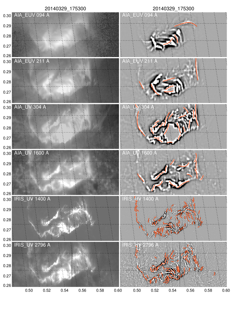
Figure 1: Original EUV and UV images are shown in intensity (left column) and as highpass-filtered fluxes (right column), with the overlaid loop segments automatically traced by OCCULT-2 (red curves in right panels). The six wavelengths include the least-saturated EUV images (94 and 211 Å) of AIA, UV images of AIA (304 and 1600 Å), and UV slit-jaw images of IRIS (1400 and 2796 Å). Note the difference in spatial resolution ($0.6\hbox{${}^{\prime\prime}$}$ for AIA and $0.166\hbox{${}^{\prime\prime}$}$ for IRIS).

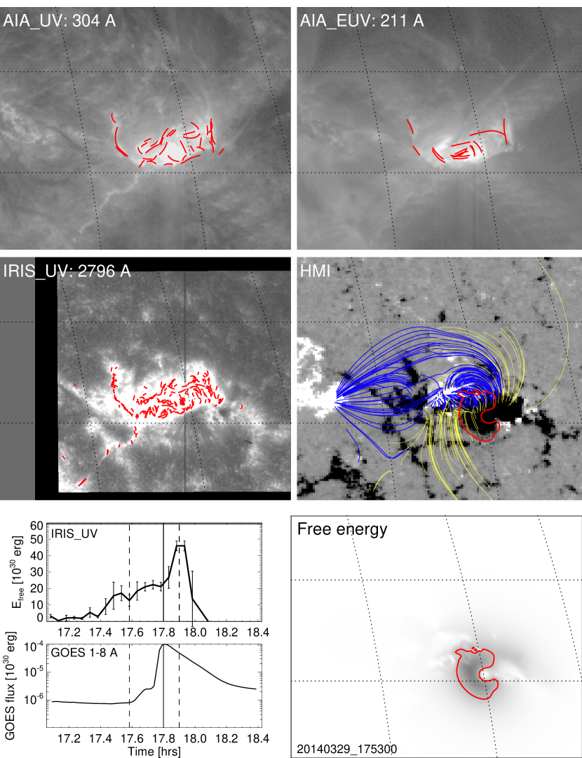
Figure 2: Highpass-filtered images from AIA 304 Å (top left), AIA 211 Å (top right), and IRIS 2796 Å (middle left), with overlaid loop tracings using an automated pattern detection code (OCCULT-2: red curves), HMI magnetogram (middle right; with range $-1472\leq B_{z}\leq 972$ G), with overlaid forward-fitted nonlinear force-free field lines (COR-NLFFF), delineating closed loops (blue curves) and open field lines (yellow curves), the spatial distribution of the free energy (bottom right), with a 50% contour level, the temporal evolution of the free energy measured from IRIS-UV (third left panel), and the GOES 1-8 Å light curve (bottom left panel).

A snapshot of the results of the magnetic modeling of the 2014 Mar 29 flare is shown in Figs. 1 and 2, at 17:53 UT, at the time of the flare peak. Original images of the flare region are shown on a logarithmic flux scale in Fig. 1 (left), juxtaposed to the highpass-filtered images (Fig. 1, right) that have been used for automated loop detection (red curves in Fig. 1 right panels). Fig. 2 shows an AIA EUV image sensitive to coronal temperatures (211 Å ), an AIA 304 Å (Fig. 2, top left) and an IRIS SJI image at 2796 Å (Fig. 2 middle left), both being sensitive to chromospheric and transition region temperatures. The loop structures traced in these images, found with the automated pattern recognition code OCCULT-2, are indicated in red. The structures detected in IRIS images are generally shorter segments than those detected in AIA images, which is partly due to a different morphology, and partly due to the 4 times higher spatial resolution of IRIS.

The geometric 2D coordinates of the automated loop tracings constrain the best fit of the NLFFF solution, which is shown together with the HMI magnetogram in Fig. 2 (middle right panel), (from which the NLFFF code uses only the LOS component). We see that the active region contains closed loops (blue curves) in the eastern dipolar part, while there are mostly open field lines in the western dipolar spot group, except for a small bipolar arcade in the core, where most of the flare action occurs. Integrating the free magnetic energy in every LOS, we created a free energy map (Fig. 2 bottom right), which reveals that the largest amount of free energy is concentrated in a semi-circular configuration surrounding the penumbra of the main western sunspot. We show the 50% contours of the free energy map $E_{free}(x,y,t)$ at 17:53 UT, shortly after the flare peak, overlaid on the magnetogram (Fig. 2 middle right panel, red contour), which is essentially identical with the location of the dissipated magnetic energy (i.e., the difference of the free energy between flare start and end). The eastern part of the semi-circular energy dissipation structure is cospatial with the location where 30-70 keV non-thermal hard X-ray emission was detected with RHESSI, as well as enhanced (hydrogen Balmer) white light continuum with IRIS 1400 Å (see Fig. 1 of Heinzel and Kleint 2014). In any case, the spatial map of the free energy localizes the footpoint areas of the flare loops that undergo magnetic reconnection. We find essentially identical free energy maps for coronal (AIA EUV wavelengths) and chromospheric or transition region (AIA UV and IRIS wavelengths) loop tracers, which implies that the magnetic information of the nonpotential field $B_{np}(x,y,t)$ and free energy $E_{free}(x,y,t)$ is imprinted in field-aligned structures that can be observed in the chromosphere, the transition region, and in the corona.

A new result of this study is that we extended nonpotential magnetic modeling from the corona down to the transition region and chromosphere, by calculating NLFFF solutions from three different wavelength sets, i.e., AIA-EUV, AIA-UV, and IRIS-UV. We show the resulting evolution of the magnetic energies calculated from these three wavelength sets in Fig. 3, performed in time steps of $\Delta t=0.05$ hrs (3 min) during the flare time interval (with 0.5 hrs margin before and after). Error bars of the free energy measurements are estimated from 3 different loop selection criteria (defined by the level of flux variability along each detected loop segment, $q_{ripple}=0.4,0.6,0.8$). We find that the free energy peaks at a value of $E_{free}\approx(45\pm 2)\times 10^{30}$ erg for all three wavelength sets. All three evolutions of free energies peak consistently within a few minutes after the GOES-based flare peak time (Fig. 3, bottom panel). Both the AIA-EUV and AIA-UV wavelength sets exhibit a step-wise drop of the free energy within 10-20 min after the flare peak, while this step could be verified in the IRIS data partially only, due to an observing sequence that unfortunately ends at 17:54:19 UT. Nevertheless, both the coronal and the chromospheric data exhibit a consistent drop in free energy, by an average amount of $\Delta E_{free}\approx(29\pm 3)\times 10^{30}$ erg, which indicates that the helically twisted magnetic field lines relax to a state of lower twist in both the corona and the chromosphere, because the COR-NLFFF solution is most sensitive to vertical currents and the associated helical twist around vertical twist axes. This is the first quantitative measurement that demonstrates in both the chromosphere and corona that the dissipated magnetic energy in a flare is caused by untwisting of (helically-twisted) stressed field lines.

4 DISCUSSION

4.1 Chromospheric Magnetic Field Tracers

Coronal loops are most conspicuously seen in EUV wavelength images with a temperature sensitivity in the $T_{e}\approx 1-2$ MK temperature range, such as in the Fe IX (171 Å) and in the Fe XII (193 Å) line, and to a lesser extent in the weaker Fe XIV (211 Å) and Fe XVI (355 Å) lines (Table 1), which all are most useful in constraining theoretical magnetic field models, such as calculated with the COR-NLFFF code (Aschwanden 2013a) or with a Grad-Rubin NLFFF method (Malanushenko et al. 2014). In the temperature regime of the photosphere, chromosphere, and transition region, which ranges from $T_{e}=5000$ K to $T_{e}\lower 1.72218pt\hbox{$\;\buildrel<\over{\scriptstyle\sim}\;$}1$ MK, we expect to see cooler loops or the footpoints of hotter coronal loops, which manifest themselves as a reticulated “moss” structure (Berger et al. 1999; De Pontieu et al. 1999). These chromospheric structures appear to be more irregular and fragmented than the smooth curvi-linear loop structures seen in the corona. Experiments to use the directions of H$\alpha$ fibrils to constrain NLFFF solutions have been undertaken by Wiegelmann et al. (2008), a method that became to be known as pre-processing, which supposedly makes the photospheric 3D vector field more force-free and provides then a more suitable near force-free boundary for NLFFF extrapolation methods. Due to regions with high plasma $\beta$-parameters and non-magnetic forces in the chromosphere, one cannot expect to model the chromospheric field correctly under the force-free assumption, neither with PHOT-NLFFF nor with COR-NLFFF codes.

Alternatively, we explore here for the first time the method of using (automatically detected) chromospheric structures to measure the local directivity of the magnetic field, which is then used to constrain a nonpotential magnetic field (COR-NLFFF) solution in an active region during a major flare. We use UV images in several wavelengths, such as the He II (304 Å) and C IV (1600 Å) lines from AIA/SDO, and the Mg II (2796 Å) and Si IV (1400 Å) lines from IRIS, which all exhibit some segments of loop-like features in the chromosphere and transition region, and thus may contain some information on the local magnetic field direction. Since the OCCULT-2 code is designed to detect curvi-linear loop structures with large curvature radii, the more irregular and inhomogeneous structures detected in the transition region and chromosphere are more challenging for automated detection of magnetic field directions, and thus it is not clear how useful they are for magnetic field modeling. However, our experiment demostrates that we detect a consistent evolution of the free energy $E_{free}(t)$ during the investigated flare in both coronal EUV and chromospheric UV wavelengths (Fig. 3), within the uncertainties of the measurements. The biggest challenge is to distinguish between contiguous field-aligned structures (segments of loops or filaments), curvi-linear aggregations of “moss”-like structures, and curved flare ribbons.

4.2 Energy Dissipation in Flares

The coronal and/or chromospheric feature tracing provides field directions, which can be used to calculate the nonpotential magnetic field ${\bf B}({\bf x})$ in a computation box that encompasses an active region or flare region. The volume integral of the free energy, $E_{free}(t)=(1/8\pi)\int B_{np}(x,y,t)^{2}-B_{p}(x,y,t)^{2}\ dx\ dy$, is ideally expected to have a higher level of free energy before the flare, and to drop to a lower level after the flare (e.g., Jing et al. 2009). We indeed find a step-wise decrease of the free energy after the flare, which defines the total dissipated magnetic energy during the flare, and is found to have a value of $\Delta E_{free}=E_{free}(t_{start})-E_{free}(t_{end})\approx(29\pm 3)\times 10^{30}$ erg here. This value is indeed typical for an X-class flare (Aschwanden et al. 2014). The apparent increase of the free energy before the flare peak time has been interpreted as an illumination effect, caused by chromospheric evaporation that fills up flare loops, whereby their helical twist becomes visible (Aschwanden et al. 2014). The dissipated magnetic energy is an important physical parameter for flare models, because it sets rigorous upper limits on other secondary flare energy conversions (thermal and nonthermal energy, kinetic energy of CMEs, etc.), it constrains the number problem for particle acceleration, and constrains physical scaling laws for magnetic reconnection processes. It is therefore imperative to establish a reliable method for the determination of nonpotential magnetic energies. A comparison of potential, nonpotential, and free energies between PHOT-NLFFF and COR-NLFFF codes has been conducted in a recent statistical study, where it was found that the dissipated flare energies determined with PHOT-NLFFF and COR-NLFFF methods disagree up to a factor of 10 (Aschwanden et al. 2014). At this point it is not clear what the largest source of uncertainties is. It is possible that the pre-processing of photospheric vector field data in the PHOT-NLFFF method introduces an over-smoothing and leads to an underestimation of magnetic energies (Sun et al. 2012). Alternatively, mis-detections or sparseness of field-aligned structures with the OCCULT-2 code could spoil the optimization of force-free $\alpha$-parameters in the COR-NLFFF code. However, the consistent result of the evolution of the free energy found in this study from both coronal and chromospheric images yields an independent test and corroboration of the COR-NLFFF method.

5 CONCLUSIONS

We calculated the time evolution of the free energy $E_{free}(t)$ during the 2014-Mar-29 flare, the first X-class flare detected by IRIS. We used HMI/SDO data to compute the potential field, and AIA/SDO and IRIS images to delineate the geometry of coronal loop segments in EUV wavelengths, as well as to delineate magnetic field directions from automatically traced structures seen in the transition region and chromosphere in UV wavelengths.

The major result of this study is that we find a similar evolution of the free energy for both coronal and chromospheric structures, peaking at a free energy of $E_{free}(t_{peak})\approx(45\pm 2)\times 10^{30}$ erg, which decreases by an amount of $\Delta E_{free}\approx(29\pm 3)\times 10^{30}$ erg in the flare decay phase, and thus represents the total magnetic energy dissipated during this X-class flare. The consistency of magnetic energy measurements from both coronal and chromospheric tracers represents an independent test and corroboration of the COR-NLFFF method. The COR-NLFFF code provides also maps of dissipated flare energies, which enables us to localize and map out magnetic reconnection regions during solar flares in great detail, which is the subject of future studies.

Table 1: Instruments and wavelengths used in the present analysis.

instrument	Wavelength	Atomic Lines	Temperature range
	$[\AA]$		$\log(T[K])$
Chromosphere and
Transition Region:
IRIS	2796	Mg II h/k	3.7-4.2
IRIS	1330	C II	3.7-7.0
IRIS	1400	Si IV	3.7-5.2
AIA	304	He II	4.7
AIA	1600	C IV	5.0
Corona:
AIA	171	Fe IX	5.8
AIA	193	Fe XII, XXIV	6.2, 7.3
AIA	211	Fe XIV	6.3
AIA	355	Fe XVI	6.4
AIA	94	Fe XVIII	6.8
AIA	131	Fe VIII, XXI	5.6, 7.0

Figure 3: Time evolution of the free energy as measured from AIA in EUV wavelengths (top panel), from AIA UV wavelengths (second panel), from IRIS UV wavelengths (third panel), along with the GOES 1-8 Å flux (solid linestyle in bottom panel) and GOES time derivative (dashed linestyle in bottom panel). The errors of the free energies are estimated from 3 different loop selections (fluctuation thresholds of 40%, 60%, and 80%.) The start, peak, and end time of the GOES event is indicated with vertical lines.

References

- (1)
- (2) Aschwanden, M.J., Lee,J.K., Gary,G.A., Smith,M., and Inhester,B. 2008, SP 248, 359.
- (3) Aschwanden, M.J. 2010, Solar Phys. 262, 399.
- (4) Aschwanden, M.J. 2013a, Solar Phys. 287, 323.
- (5) Aschwanden, M.J. 2013b, Solar Phys. 287, 369.
- (6) Aschwanden, M.J. and Malanushenko, A. 2013, Solar Phys. 287, 345.
- (7) Aschwanden, M.J., Boerner, P., Schrijver, C.J., and Malanushenko, A. 2013a, Solar Phys. 283, 5.
- (8) Aschwanden, M.J., De Pontieu, B., and Katrukha, E.A. 2013b, Entropy 15(8), 3007.
- (9) Aschwanden, M.J,, Xu, Y., and Jing, J. 2014, ApJ, 797, 50.
- (10) Berger, T.E., De Pontieu, B., Fletcher, L., Schrijver, C.J., Tarbell,T.D., and Title, A.M. 1999, Solar Phys. 190, 409.
- (11) De Pontieu, B., Berger, T.E., Schrijver, C.J., and Title, A.M. 1999, Solar Phys. 190, 419.
- (12) De Pontieu, B., Title, A.M., Lemen, J.R., Kushner, G.D., Akin, D.J., Allard, B., Berger, T., Boerner, P., et al. 2014, Solar Physics 289, 2733.
- (13) DeRosa, M.L., Schrijver, C.J., Barnes, G., Leka, K.D., Lites, B.W., Aschwanden, M.J., Amari,T., Canou, A., et al. 2009, ApJ 696, 1780.
- (14) Emslie, A.G., Dennis, B.R., Shih, A.Y., Chamberlin, P.C., Mewaldt, R.A., Moore, C.S., Share, G.H., Vourlidas, A., et al. 2012 ApJ 759, 71.
- (15) Gary, G.A. 2001, Solar Phys. 203, 71.
- (16) Heinzel, P. and Kleint, L. 2014, ApJL 794, L23.
- (17) Jing, J., Chen, P.F., Wiegelmann, T., Xu, Y., Park, S.-H., and Wang, H. 2009, ApJ 696, 84.
- (18) Judge, P.G., Kleint, L., Donea, A., Sainz-Dalda A., and Fletcher, L. 2014, ApJ 796, 85.
- (19) Lemen, J.R., Title, A.M., Akin, D.J., Boerner, P.F., Chou, C., Drake, J.F., Duncan, D.W., Edwards, C.G., et al. 2012, Solar Phys. 275, 17.
- (20) Malanushenko, A., Schrijver, C.J., DeRosa, M.L., and Wheatland, M.S. 2014, ApJ 783, 102.
- (21) Metcalf, T.R., Jiao, L., Uitenbroek, H., McClymont, A.N., and Canfield, R.C. 1995, ApJ 439, 474.
- (22) Pesnell, W.D., Thompson, B.J., and Chamberlin, P.C. 2011, Solar Phys. 275, 3.
- (23) Priest, E.R. 1982, Solar Magnetohydrodynamics, Reidel Publishing Company, Dordrecht: Holland.
- (24) Priest, E.R. 2014, Magnetohydrodynamics of the Sun, Cambridge, UK: Cambridge University Press.
- (25) Scherrer, P.H., Schou, J., Bush, R. I., Kosovichev, A.G., Bogart, R.S., Hoeksema, J.T., Liu, Y., Duvall, T.L., et al. 2012, Solar Phys. 275, 207.
- (26) Schrijver, C.J., DeRosa, M., Metcalf, T.R., Liu, Y., McTiernan, J., Regnier, S., Valori, G., Wheatland, M.S., and Wiegelmann,T. 2006, Solar Phys. 235, 161.
- (27) Schrijver, C.J., DeRosa, M.L., Metcalf, T., Barnes, G., Lites, B., Tarbell, T., McTiernan, J., Valori, G. et al. 2008, ApJ 675, 1637.
- (28) Sun, X., Hoeksema, J.T., Liu, Y., Wiegelmann, T., Hayashi, K., Chen, Q., and Thalmann, J. 2012, ApJ 748, 77.
- (29) Wiegelmann, T. 2004, Solar Phys. 219, 87.
- (30) Wiegelmann, T., Inhester, B., and Sakurai, T. 2006, Solar Phys. 233, 215.
- (31) Wiegelmann, T., Thalmann, T., Schrijver, C.J., DeRosa,M.L., and Metcalf,T.R. 2008, Solar Phys. 247, 249.
- (32) Young, P.R., Tian, H., and Jaeggli, S. 2015, ApJ 799, 218.