Coherent Averaging

Abstract

We investigate in detail a recently introduced “coherent averaging scheme” in terms of its usefulness for achieving Heisenberg limited sensitivity in the measurement of different parameters. In the scheme, $N$ quantum probes in a product state interact with a quantum bus. Instead of measuring the probes directly and then averaging as in classical averaging, one measures the quantum bus or the entire system and tries to estimate the parameters from these measurement results. Combining analytical results from perturbation theory and an exactly solvable dephasing model with numerical simulations, we draw a detailed picture of the scaling of the best achievable sensitivity with $N$, the dependence on the initial state, the interaction strength, the part of the system measured, and the parameter under investigation.

I Introduction

Averaging data is a common procedure for noise reduction in all quantitative sciences. One measures the noisy quantity $N$ times, and then calculates the mean value of the $N$ samples. Assuming that the useful signal part is the same for each run of the experiment, the random noise part averages out and leads to an improvement by a factor $\sqrt{N}$ of the signal-to-noise ratio (SNR). Instead of measuring the same sample $N$ times, one may of course also measure $N$ identically prepared samples in parallel, in which case we will think of them as “probes”. A lot of excitement has been generated by the realization that in principle one may improve upon the $\sqrt{N}$ factor by probes that are not independent, but in an entangled state. It was shown Giovannetti04 that with such “ quantum enhanced measurements” the SNR can be improved by up to a factor $N$. Unfortunately, on the experimental side, decoherence issues have limited the quantum enhancement to very small values of $N$ Leibfried05 ; Nagata07 ; Higgins07 . For practical purposes it is therefore often more advantageous to stay with a classical protocol and increase $N$ Pinel12 . Since the decoherence problem is very difficult to solve, one should think about alternative ways of increasing the SNR through the use of quantum effects. One such idea is “coherent averaging”. The original scheme, first introduced in Braun10.2 ; Braun11 and named as such in braun_coherently_2014 , works in the following way: instead of measuring the $N$ probes individually, one lets them interact coherently with a $N+1$st system (a “ quantum bus”) and then reads out the latter. In this way, quantum mechanical phase information from the $N$ probes can accumulate in the quantum bus, and this can improve the SNR also by a factor $N$, even when using an initial product state (see Fig.1). A physical example considered in detail was the coupling of $N$ atoms to a single leaky cavity mode, which allowed to measure the length of the cavity with a precision scaling as $1/N$, which corresponds to the above SNR $\propto N$. This scaling is the long-sought Heisenberg-limit (HL), contrasting with the $1/\sqrt{N}$ scaling characteristic of the standard, classical averaging regime, also called standard quantum limit (SQL).

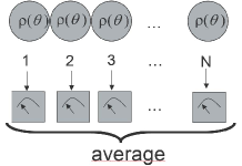
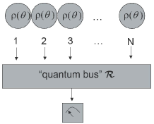
Figure 1: Classical averaging (left) versus coherent averaging (right). In coherent averaging, the $N$ probes are not read out individually and the results averaged, but one lets the probes coherently interact with a quantum bus, and then either measures the latter, or a global observable of the entire system. The parameter to be estimated can parametrize the probes, the quantum bus, or the interaction.

So far, however, the method was limited to estimating a parameter linked to the interaction of the $N$ probes with the quantum bus. This makes comparison of the performance with and without the coupling to the quantum bus impossible, as in the latter case the parameter to be estimated does not even exist. In the present work we go several steps further. Firstly, we extend the scheme to estimating a parameter that characterizes the probes themselves, or the quantum bus itself. Secondly, we analyze in detail conditions for the observation of the HL scaling by systematically studying strong, intermediate and weak coupling regimes. Numerical simulations are used in order to verify and extend results from analytical perturbation-theoretical calculations. Thirdly, we investigate the question which part of the system should be measured.

Note that achieving HL scaling of the sensitivity in coherent averaging with an initial product state is not in contradiction with the well-known no-go-theorem Giovannetti04 which is at the base of the often held believe that entanglement is necessary for surpassing the SQL. The reason is that in Giovannetti04 the Hamiltonian is assumed to be simply a sum of Hamiltonians of independent subsystems with no interactions, which is a natural assumption when coming from classical averaging. Meanwhile, however, several other ways have been found to bypass the requirements of the theorem and thus avoid the use of entanglement for HL sensitivity, notably the use of interactions (also known as non-linear scheme) luis_quantum_2007 ; napolitano_interaction-based_2011 , multi-pass schemes Higgins07 , or the coding of a parameter other than through unitary evolution (e.g. thermodynamic parameters such as the chemical potential) marzolino_precision_2013 .

From a perspective of complex quantum systems, the models that we study are typical decoherence models: the quantum bus may be considered an environment for the $N$ probes, or vice versa. However, in general we will assume that we can control both probes and quantum bus, and in particular prepare them in well defined initial states which we take as pure product states or thermal states.

II Models and methodology

II.1 Models

The systems we are interested in have the following general structure depicted in Fig.1. The corresponding Hamiltonian can be written as

$$H = \delta H_{0}+\varepsilon H_{\text{int}}$$ (1)

$$= \delta\left(\sum_{i=1}^{N}H_{i}(\omega_{1})+H_{R}(\omega_{0})\right)+\varepsilon\left(\sum_{i,\nu}S_{i,\nu}(x)\otimes R_{\nu}\right)\,,$$ (2)

where $H_{0}$ contains the “free” part (probes and quantum bus), and $H_{\text{int}}$ the interaction between the probes and the quantum bus. We have introduced two dimensionless parameters $\delta$ and $\varepsilon$ which we will use to reach the different regimes of strong, intermediate, and weak interaction. In the second line we specify the Hamiltonians $H_{i}$ for $N$ non-interacting probes which we assume to depend on the parameter $\omega_{1}$, and the Hamiltonian $H_{R}$ of the quantum bus (or “reservoir” in the language of decoherence theory) which depends on the parameter $\omega_{0}$. The interaction has the most general form of a sum of tensor products of probe-operators and quantum-bus-operators and we assume that it depends on a single parameter $x$.

As specific examples of systems of this type we consider spin-systems, where both the probes and the quantum bus are spins-1/2 (or qubits) and thus described by Pauli-matrices $X,Y,Z$. Without restriction of generality, we can take $H_{i}=\frac{\omega_{1}}{2}Z^{(i)}$ for the $i$-th probe, and $H_{R}=\frac{\omega_{0}}{2}Z^{(0)}$ ($\hbar=1$ throughout the paper), where the bracketed superscripts denote the subsystem, and the zeroth subsystem is the quantum bus. For the interaction we focus on two different cases: an exactly solvable pure dephasing model with

$$H_{\text{int}}=\frac{x}{2}\sum_{i}Z^{(i)}\otimes Z^{(0)}\,,$$ (3)

and a model that allows exchange of energy through an $XX$-interaction, given by

$$H_{\text{int}}=\frac{x}{2}\sum_{i}X^{(i)}\otimes X^{(0)}\,.$$ (4)

We refer to these two models as $ZZZZ$ and $ZZXX$ models.

II.2 Initial state

Given the difficulty of producing entangled states and maintaining them entangled, we consider here pure initial product states with all the probes in the same state, which may be different from the state of the quantum bus. For the spin-systems we parametrize these states as

$$|\,\psi_{0}\,\rangle = \left(\bigotimes_{i}^{N}|\,\varphi\,\rangle_{i}\right)\otimes|\,\xi\,\rangle$$ (6)

$$= \left(\cos(\alpha)|\,0\,\rangle+\sin(\alpha){\rm e}\,^{\mathrm{i}\phi}|\,1\,\rangle\right)^{\otimes N}$$

$$\otimes\left(\cos(\beta)|\,0\,\rangle+\sin(\beta){\rm e}\,^{\mathrm{i}\varphi}|\,1\,\rangle\right)\,,$$

where $|\,0\,\rangle,|\,1\,\rangle$ denote “computational basis states”, i.e. $Z|\,0\,\rangle=|\,0\,\rangle$ and $Z|\,1\,\rangle=-|\,1\,\rangle$ for any spin. Eq.(6) implies that in the subspace of the probes, the initial state is a $SU(2)$ angular momentum coherent state of spin $j=N/2$. Since both initial state and the considered Hamiltonians are symmetric under exchange of the $N$ probes, this symmetry is conserved at all times, and allows for a tremendous reduction of the dimension of the relevant Hilbert space: from $2^{N+1}$ to only $2(N+1)=2(2j+1)$ dimensions. The corresponding basis in the probe-Hilbert space is the usual joint-eigenbasis $|j,m\rangle$ of total spin and its $z$-component. We will omit the label $j$ and have thus the representation of $|\,\psi_{0}\,\rangle$ in the symmetric sector of Hilbert space

$$|\,\psi_{0}\,\rangle = \sum_{m=-N/2}^{N/2}\sqrt{\binom{N}{m+N/2}}\cos(\alpha)^{N/2+m}(\sin(\alpha){\rm e}\,^{\mathrm{i}\phi})^{N/2-m}$$ (7)

$$\left(\cos(\beta)|\,m,0\,\rangle+\sin(\beta){\rm e}\,^{\mathrm{i}\varphi}|\,m,1\,\rangle\right)\;.$$

For the ZZZZ model we also consider thermal states of the probes, see eq.(37) below. In other contexts, the above models have been called spin-star models, and analyzed with respect to degradation of channel capacities and entanglement dynamics PhysRevA.81.062353 ; ferraro_entanglement_2009 ; hamdouni_exactly_2009 .

II.3 Quantum parameter estimation theory

The question of how precisely one can measure the parameters $\omega_{1},\omega_{0}$ and $x$ is addressed most suitably in the framework of quantum parameter estimation theory (q-pet). Q-pet builds on classical parameter estimation theory, which was developed in statistical analysis almost a century ago Rao1945 ; Cramer46 . There one considers a parameter–dependent probability distribution $p(A,\theta)$ of some random variable $A$. The form of $p(A,\theta)$ is known, and the task is to provide the best possible estimate of the parameter $\theta$ from a sample of $n$ values $A_{i}$ drawn from the distribution. For this purpose, one compares different estimators, i.e. functions $\theta_{\rm est}(A_{1},\ldots,A_{n})$ that depend on the measured values $A_{i}$ (and nothing else), and give as output an estimate $\theta_{\rm est}$ of the true value of $\theta$. Since the $A_{i}$ are random, so is the estimate. Under “best estimate” one commonly understands an estimate that fluctuates as little as possible, while being unbiased at the same time.
In quantum mechanics (QM), the task is to estimate a parameter $\theta$ that is coded quite generally in a density matrix, $\rho(\theta)$. One has then the additional degree of freedom to measure whatever observable (or more generally: positive-operator valued measure (POVM)Peres93 ). The so-called quantum Cramér-Rao bound is optimized over all possible POVM measurements and data analysis schemes in the sense of unbiased estimators. It gives the smallest possible uncertainty of $\theta_{\rm est}$ no matter what one measures (as long as one uses a POVM measurement — in particular, post selection is not covered, see braun_precision_2014 for an example), and no matter how one analyzes the data (as long as one uses an unbiased estimator). At the same time it can be reached at least in principle in the limit of a large number of measurements. The quantum Cramér-Rao bound (QCR) has therefore become the standard tool in the field of precision measurement. It is given by

$$\text{Var}(\theta_{\text{est}})\geq\frac{1}{MI_{\theta}}\quad\;,$$ (8)

where Var($\theta_{\text{est}}$) is the variance of the estimator, $I_{\theta}$ the Quantum Fisher Information (QFI), and $M$ the number of independent measurements. A basis–independent form of $I_{\theta}$ reads Paris09

$$I_{\theta}=2\int_{0}^{\infty}ds\,\text{tr}\left[\partial_{\theta}\rho_{\theta}{\rm e}\,^{-\rho_{\theta}s}\partial_{\theta}\rho_{\theta}{\rm e}\,^{-\rho_{\theta}s}\right]\,.$$ (9)

In the eigenbasis of $\rho_{\theta}$, i.e. for $\rho_{\theta}=\sum_{r}p_{r}|\,\psi_{r}\,\rangle\langle\,\psi_{r}\,|$ we obtain

$$I_{\theta}=\sum_{r}\frac{(\partial_{\theta}p_{r})^{2}}{p_{r}}+2\displaystyle\sum_{\begin{subarray}{c}n,m\end{subarray}}\frac{(p_{n}-p_{m})^{2}}{p_{n}+p_{m}}\left|\langle\,\psi_{n}\,|\,\partial_{\theta}\,\psi_{m}\,\rangle\right|^{2}\;,$$ (10)

where the sums are over all $r$ and $n,m$ such that the denominators do not vanish. It is possible to give a geometrical interpretation to the QFI, namely in terms of statistical distance. To this end one defines the Bures distance between two states $\rho$ and $\sigma$ as

$$d_{B}(\rho,\sigma)=\sqrt{2}\sqrt{1-\text{tr}[(\rho^{1/2}\sigma\rho^{1/2})^{1/2}])}\;.$$ (11)

In the case of two pure states $\phi$, $\psi$, we have

$$d_{B}(|\,\phi\,\rangle,|\,\psi\,\rangle)=\sqrt{2}\sqrt{1-|\langle\,\phi\,|\,\psi\,\rangle|)}\;.$$ (12)

The Bures distance was shown to be related to the QFI by Braunstein94

$$I_{\theta}=4d_{B}^{2}(\rho(\theta),\rho(\theta+d\theta))/d_{\theta}^{2}\;.$$ (13)

It provides an intuitive interpretation to the best sensitivity with which a parameter can be estimated in the sense that what matters is how much two states distinguished by an infinitesimal difference in the parameter $\theta$ differ, where the difference is measured by their Bures distance. In the case of a pure state, the QFI is equal to

$$I_{\theta}=4(\langle\,\partial_{\theta}\,\psi(\theta)\,|\,\partial_{\theta}\,\psi(\theta)\,\rangle-|\langle\,\psi(\theta)\,|\,\partial_{\theta}\,\psi(\theta)\,\rangle|^{2})\;.$$ (14)

II.4 Perturbation theory

It is clear that the model (1) cannot be solved in all generality. One way of making progress is to use perturbation theory. This can be done in two ways: In the standard use of perturbation theory one solves the Schrödinger equation for the free Hamiltonian $H_{0}$ and then treats the interaction $H_{\rm int}$ in perturbation theory, provided that the interaction is small enough. In the regime of strong interaction, one can do the opposite thing: solve the pure interaction problem first, and then calculate the additional effect of the free Hamiltonian as a perturbation. Formally this does not make a big difference. More important, already on the level of the expression for the QFI, is the question whether the parameter to be estimated enters in the perturbation or in the dominant part of the Hamiltonian. We call the perturbation theory relevant for these two cases PT1 and PT2, respectively.

To better understand the difference between PT1 and PT2, consider a Hamiltonian containing two parts where one of them depends on a parameter that we want to estimate,

$$H(\theta)=H_{1}(\theta)+H_{2}\;,$$ (15)

and the state

$$|\,\psi(\theta)\,\rangle=\exp(-\mathrm{i}tH(\theta))|\,\psi_{0}\,\rangle\;.$$ (16)

In PT1 we switch to the interaction picture with respect to $H_{2}$,

$$H_{1,I}(\theta,t)={\rm e}\,^{\mathrm{i}tH_{2}}H_{1}(\theta){\rm e}\,^{-\mathrm{i}tH_{2}}\;.$$ (17)

Under the conditions that $|H_{1,I}t|,|{H_{1,I}}^{\prime}t|\ll 1$ and $||H_{1}(\theta)||\ll||H_{2}||$ we can use second order perturbation theory in order to calculate the QFI Braun11 ,

$$I_{\theta}=4\int_{0}^{t}\int_{0}^{t}dt_{1}dt_{2}K_{|\,\psi_{0}\,\rangle}({H_{1,I}}^{\prime}(\theta,t_{1}),{H_{1,I}}^{\prime}(\theta,t_{2}))\;,$$ (18)

with $K_{|\,\psi\,\rangle}(A,B)=\langle\psi\,|\,AB\,|\,\psi\rangle-\langle\psi\,|\,A\,|\,\psi\rangle\langle\psi\,|\,B\,|\,\psi\rangle$. If the free Hamiltonian commutes with the interaction Hamiltonian (as is the case in the ZZZZ model), and under the assumptions that $[H_{1}(\theta),{H_{1}(\theta)}^{\prime}]=0$, one can calculate the QFI exactly,

$$I_{\theta}=4t^{2}K_{|\,\psi_{0}\,\rangle}({H_{1}}^{\prime}(\theta),{H_{1}}^{\prime}(\theta))\;.$$ (19)

The last term of the right hand side is the variance of ${H_{1}}^{\prime}(\theta)$ in the initial state, and we thus recover a well known result in Q-pet braunstein_generalized_1996 . At the same time, eq.(18) tells us that the QFI is of second order in the perturbation.

In PT2, we do the opposite: estimate the parameter linked to the Hamiltonian that dominates. With the notation of eq.(15) this means that we try to estimate the parameter $\theta$, considering that $|H_{2,I}t|,|{H_{2,I}}^{\prime}t|\ll 1$ and $||H_{1}(\theta)||\gg||H_{2}||$, with

$$H_{2,I}(\theta,t)={\rm e}\,^{\mathrm{i}tH_{1}(\theta)}H_{2}{\rm e}\,^{-\mathrm{i}tH_{1}(\theta)}\;.$$ (20)

In this case, the result (18) does not apply anymore. Indeed, to obtain (18) we calculated the overlap $\langle\,\psi(\theta,t)\,|\,\psi(\theta+d\theta,t)\,\rangle$, which equals $\langle\,\psi_{1,I}(\theta,t)\,|\,\psi_{1,I}(\theta+d\theta,t)\,\rangle$. Now we need

$$\langle\,\psi_{2,I}(\theta,t)\,|{\rm e}\,^{\mathrm{i}tH_{1}(\theta)}{\rm e}\,^{-\mathrm{i}tH_{1}(\theta+d\theta)}|\,\psi_{2,I}(\theta+d\theta,t)\,\rangle\,.$$ (21)

Here we have defined

$$|\,\psi_{j,I}(\theta,t)\,\rangle=T\left[\exp(-\mathrm{i}\int_{0}^{t}H_{j,I}(t^{\prime})dt^{\prime})\right]|\,\psi_{0}\,\rangle$$

for $j=1,2$, and $T$ is the time-ordering operator. In this case, the lowest order term that appears in the expansion of the QFI is the unperturbed term,

$$I_{\theta}=4t^{2}\left(\langle\psi_{0}\,|\,{H_{1}}^{\prime}(\theta)^{2}\,|\,\psi_{0}\rangle-\langle\psi_{0}\,|\,{H_{1}}^{\prime}(\theta)\,|\,\psi_{0}\rangle^{2}\right).$$ (22)

The formal range of validity is now given by $|H_{2,I}t|,|{H_{2,I}}^{\prime}t|\ll 1$ and $||H_{1}(\theta)||\gg||H_{2}||$. The first and second order terms are too cumbersome to be reported here. But since in the formal range of validity of the perturbation theory they have to remain small in comparison to the zeroth order term, the scaling of the QFI with $N$ will be given anyhow by the zeroth order term (22).

For practical applications and in the spirit of the original “coherent averaging” scheme, we are also interested in the sensitivity that can be achieved by only measuring the quantum bus. To this end, we calculate the reduced density matrix by tracing out the probes, and then the QFI for the corresponding mixed state which we call “local QFI” $I_{\theta}^{(0)}$. Since tracing out a subsystem corresponds to a quantum channel under which the Bures distance is contractive Bengtsson06 , we have $I_{\theta}\geq I_{\theta}^{(0)}$.

In general, the calculation of the QFI for a mixed state is rather difficult, as one has to diagonalize the density matrix twice (either for two slightly different values of the parameter for calculating the derivatives (10), or for calculating $\rho^{1/2}$ and $(\rho^{1/2}\sigma\rho^{1/2})^{1/2}$). Techniques for bounding the QFI for mixed states have been developed in the literature escher_general_2011 ; Kolodynski10 . Here, we only calculate the QFI for the mixed state of a single qubit, which is easily achievable numerically.

Another important practical question is with which measurement the optimal sensitivity can be achieved. In principle, the answer can be found from the QFI formalism Braunstein94 ; Paris09 . Here we follow the strategy of considering local von Neumann measurements of the quantum bus and comparing the achievable sensitivity to the optimal one. If a von Neumann measurement with a Hermitian operator $B$ is performed, one can show that an estimator $\theta_{\rm est}(B_{1},\ldots,B_{M})=f^{-1}(\sum_{i=1}^{M}B_{i}/M)$ with $f(\theta)=\langle\psi(\theta)|B|\psi(\theta)\rangle$ leads to first order in the expansion of $f^{-1}$ to an uncertainty (standard deviation) of $\theta_{\rm est}$ given by

$$\delta_{\theta}^{B}=\frac{\sqrt{{\rm Var}(B)}}{\sqrt{M}|\partial_{\theta}\langle\,B\,\rangle|}\;$$ (23)

with ${\rm Var}(B)=\langle\,B^{2}\,\rangle-\langle\,B\,\rangle^{2}$ (see eq.(9.16) in kay_fundamentals_1993 ). This “method of the first moment” can always be rendered locally unbiased by adding a shift to $\theta_{\rm est}$. The uncertainty $\delta_{\theta}^{B}$ corresponds to the minimal change of $\theta$ that shifts the distribution of the $B_{i}$ by one standard deviation, assuming that the shift is linear in $d\theta$ for small $d\theta$. Since $\delta_{\theta}^{B}$ is based on a particular estimator, we have $(\delta_{\theta}^{B})^{-2}\leq MI_{\theta}$.

We call the local observable of the quantum bus $A^{(0)}=\mbox{\hskip 3.00003ptl1}^{\otimes N}\otimes A$, and $\delta_{x}^{A^{(0)}}$ and $\delta_{\omega_{1}}^{A^{(0)}}$ the corresponding uncertainties for the estimation of $x$ and $\omega_{1}$. The QFI of the reduced density matrix for the quantum bus alone will be denoted $I_{x}^{(0)}$ and $I_{\omega_{1}}^{(0)}$. We have $MI_{\theta}\geq MI_{\theta}^{(0)}\geq(\delta_{\theta}^{A})^{-2}=(\delta_{\theta}^{A^{(0)}})^{-2}$. The last step follows from $\langle A^{(0)}\rangle=\langle A\rangle$ for any quantum state.

II.5 Numerics

When $\varepsilon H_{\rm int}$ and $\delta H_{0}$ are of the same order, both forms of perturbation theory typically break down. Unless one has an exactly solvable model (such as the ZZZZ model), one has to rely on numerics. In addition, we use numerics to test all our analytical results. The perturbative results are, in general, limited to a finite range of $N$, such that when one wants to make a statement about the scaling of the sensitivity of a measurement with $N$ for large $N$, one has to rely once more on numerics. All numerical calculations use one of the spin-Hamiltonians, eq.(3) or (4).

The numerical results are obtained by calculating the time evolution operator $U(t)=\exp(-\mathrm{i}Ht)$ for the full Hamiltonian in the Schrödinger picture, propagating the initial state (7) for two slightly different values of the parameter we are interested in ($x$, $\omega_{1}$, or $\omega_{0}$), obtain from this a numerical approximation of the derivatives of $|\psi(t)\rangle$ with respect to the parameter, and then calculate the overlaps in eq.(14). In this way, we obtain the “global QFI”, which is relevant if one has access to the entire system (i.e. probes and quantum bus). To check the stability of the numerical derivative, we calculate numerical approximations of the derivative for two different changes in the value of the parameter, $10^{-8}$ and $10^{-6}$.

For the spin-Hamiltonians considered, the reduced density matrix of the quantum bus is the density matrix of a single spin-1/2 which simplifies the calculation of the QFI. For numerical calculations we use the basis–independent form (9) of the QFI and perform the integral analytically. We also calculated $\delta_{\omega_{1}}^{A^{(0)}}$ and $\delta_{x}^{A^{(0)}}$ numerically “exactly” by directly evaluating (23).

In order to check the validity of the perturbative result, we verified that in the range of validity of the perturbation theory the difference between the exact QFI and the perturbative result scales as $\delta^{3}$ or $\varepsilon^{3}$ as function of the perturbative parameter $\delta$ or $\varepsilon$.

III Results

We now present our results for the estimation of $x$, $\omega_{0}$, and $\omega_{1}$ in the different regimes, focusing first on the global QFI. All figures shown have the parameters $\omega_{0}=1$, $\omega_{1}=1$, $t=1$, $x=1$. The initial pure state (6) is taken always with $\alpha=\pi/3$, $\beta=\pi/6$, $\phi=3\pi/8$, $\varphi=5\pi/8$ unless otherwise indicated.

III.1 Global QFI

III.1.1 Estimation of $x$

The perturbation theory for estimating $x$ for small interactions was developed in Braun11 . Inserting the form (2) in eq.(18), one finds that for identical and identically prepared systems $\mathcal{S}_{i}$ ($S_{i,\nu}=S_{\nu}$ and $|\,\varphi\,\rangle_{i}=|\,\varphi\,\rangle$) the correlation function in eq.(18) is given to lowest order in $\varepsilon$ by

$$K_{|\,\psi_{0}\,\rangle}({H_{{\rm int},I}}^{\prime}(x,t_{1}),{H_{{\rm int},I}}^{\prime}(x,t_{2}))=\\ \varepsilon^{2}\sum_{\mu,\nu}\{NK_{|\,\varphi\,\rangle}\left({S_{\nu}}^{\prime}(x,t_{1}),{S_{\mu}}^{\prime}(x,t_{2})\right)\langle\xi\,|\,R_{\nu}(t_{1})R_{\mu}(t_{2})\,|\,\xi\rangle\\ +\left.N^{2}\langle\varphi\,|\,{S_{\nu}}^{\prime}(x,t_{1})\,|\,\varphi\rangle\langle\varphi\,|\,{S_{\mu}}^{\prime}(x,t_{2})\,|\,\varphi\rangle K_{|\,\xi\,\rangle}\left(R_{\nu}(t_{1}),R_{\mu}(t_{2})\right)\right\}\;.$$ (24)

We have defined $H_{{\rm int},I}=U_{0}(t)\varepsilon H_{\rm int}U_{0}(t)^{\dagger}$ with $U_{0}(t)=\exp(\mathrm{i}\delta H_{0}t)$, and $S_{\mu}(x,t)=U_{0}(t)S_{\mu}U_{0}(t)^{\dagger}$, $R_{\mu}(t)=U_{0}(t)R_{\mu}U_{0}(t)^{\dagger}$. This implies a structure $I_{x}=\varepsilon^{2}(n_{1,x}N+n_{2,x}N^{2})+{\cal O}(\varepsilon^{3})$ of the QFI, where $n_{1,x}$ and $n_{2,x}$ can be expressed in terms of time integrals of correlation functions. However, higher orders in $\varepsilon$ limit the formal validity of the perturbation theory to sufficiently small values of $N$. Indeed, the next higher order may contain terms of the order $\varepsilon^{3}N^{3}$, which are only much smaller than the second order for $N\ll 1/\varepsilon$.

Eq.(24) allows one to establish the condition for HL scaling, namely that Braun11

$$\int_{0}^{t}\int_{0}^{t}dt_{1}dt_{2}\sum_{\mu,\nu}\langle\varphi\,|\,{S_{\nu}}^{\prime}(x,t_{1})\,|\,\varphi\rangle\langle\varphi\,|\,{S_{\mu}}^{\prime}(x,t_{2})\,|\,\varphi\rangle$$

$$\times K_{|\,\xi\,\rangle}\left(R_{\nu}(t_{1}),R_{\mu}(t_{2})\right)\neq 0.$$

Numerics for the ZZXX model confirms the perturbative result in its expected range of validity. Moreover, it also indicates that the HL scaling works beyond the formal range of validity of the PT. This is shown in Fig.2, where we compare the global QFI for measuring $x$ for weak, medium, and strong interactions.

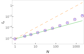
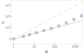
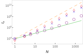
Figure 2: From left to right: Global QFI for the ZZXX model for $x$ for weak, medium, and strong interactions ($\varepsilon=0.001,\,\,\,1$, $\varepsilon=100$, and $\delta=1$). Blue X-symbols: exact numerical results. Purple circles: perturbative result (PT1). Red diamonds: zeroth order (unperturbed) term in PT2. The dashed orange (resp. green continuous) lines represent $f(N)\propto N^{2}$ (resp. $N$).

We see that PT1 works correctly for $\varepsilon N\ll 1$. For medium and strong interactions, PT1 still predicts a scaling of the global QFI proportional to $N^{2}$. While this is confirmed by the exact numerical results, the prefactors differ outside the formal range of validity of perturbation theory. The $N^{2}$ scaling is more easily observed for strong interactions than for weak ones, but Fig.2 shows that even for weak and medium interactions a $N^{2}$ component is already present. The onset of this behavior can clearly be identified in Fig.2 for $\varepsilon=0.001$ and $\varepsilon=1$.

For strong interactions, PT2 is appropriate for obtaining the QFI for $x$. The zeroth term (22) dominates in the range of validity of the perturbation theory, and leads to

$$I_{x}=\delta^{0}\varepsilon^{2}t^{2}\left(N^{2}\sin^{2}(2\alpha)\cos^{2}(2\beta)+N\cos^{2}(2\alpha)\right)+{\cal O}(\delta).$$ (25)

This implies HL scaling in the formal range of validity ($N\delta\ll 1$ and $\delta\ll\varepsilon$). Figure 2 shows that eq.(25) works well even beyond this regime. A more precise assessment of the range of validity has to consider the matrix norm of $H_{0}t$. If the largest absolute eigenvalue of $H_{i}$ is $\lambda_{\rm max}$, then PT2 is expected to work for $N\lambda_{\rm max}t\delta\ll 1$ and $\delta\ll\varepsilon$.

III.1.2 Estimation of $\omega_{1}$

The situation is similar for estimating $\omega_{1}$. PT1 (i.e. treating $\delta H_{0}$ as perturbation, such that in the interaction picture $H_{0,I}=U_{\rm int}(t)\delta H_{0}U_{\rm int}(t)^{\dagger}$ with $U_{\rm int}(t)={\rm e}\,^{\mathrm{i}\varepsilon tH_{\text{int}}}$), and assuming that $\left[R_{\nu},R_{\mu}\right]=0,\forall\nu,\mu$, leads to a correlation function to lowest order in $\delta$ given by

$$K_{|\,\psi_{0}\,\rangle} ({H_{0,I}}^{\prime}(\omega_{1},t_{1}),{H_{0,I}}^{\prime}(\omega_{1},t_{2}))=$$ (26)

$$\delta^{2}\Big{\{}N\langle\,\xi\,|\left(K_{|\,\varphi\,\rangle}\left(H_{i,I}^{(0)}(\omega_{1},t_{1}),H_{i,I}^{(0)}(\omega_{1},t_{2})\right)\right)|\,\xi\,\rangle$$

$$+ N^{2}K_{|\,\xi\,\rangle}\left(\langle\varphi\,|\,H_{i,I}^{(0)}(\omega_{1},t_{1})\,|\,\varphi\rangle,\langle\varphi\,|\,H_{i,I}^{(0)}(\omega_{1},t_{2})\,|\,\varphi\rangle\right)\Big{\}}\;;$$

with $H_{i,I}^{(0)}(\omega_{1},t_{1})=U_{\rm int}(t_{1}){H_{i}}^{\prime}(\omega_{1})U_{\rm int}^{\dagger}(t_{1})$. Note that $H_{i,I}^{(0)}(\omega_{1},t_{1})$ is still an operator on the quantum bus after sandwiching it between probe states $|\,\varphi\,\rangle$. Eq.(26) together with (18) shows that $I_{\omega_{1}}$ obeys HL scaling for $\delta\,N\ll 1$.It is easier to observe HL scaling for $\delta\ll 1$, i.e. in the regime of small free Hamiltonian or, equivalently, strong interactions, see Fig.3. For medium interactions ($\delta=1$), HL scaling is still observed, whereas for weak interactions ($\delta=100$) SQL scaling prevails at least up to $N=2000$. Formally, the range of validity of PT1 is limited here to $N\ll 1/\delta$, but numerics indicates HL scaling up to much larger $N$.

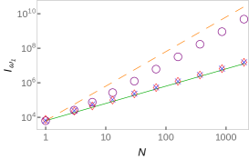
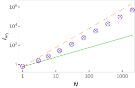
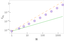
Figure 3: From left to right: Global QFI for the ZZXX model for $\omega_{1}$ for weak, medium, and strong interactions ($\delta=100,1$, $\delta=0.001$, and $\varepsilon=1$) . Blue X-symbols: exact numerical results. Purple circles: perturbative result (PT1). Red diamonds: zeroth (unperturbed) term in PT2. The dashed orange (resp. green continuous) lines represent $f(N)\propto N^{2}$ (resp. $N$).

In the formal range of validity, PT1 gives the necessary condition $\left[S_{i,\nu},H_{i}\right]\neq 0$ for observing HL scaling, as otherwise $H_{i,I}^{(0)}$ becomes proportional to the identity operator in the quantum bus Hilbert space. Numerically it can be checked that a violation of this condition indeed leads only to SQL scaling. We verified this for the ZZZX model, defined as the ZZXX model, but with a Hamiltonian $S_{i}=\frac{x}{2}Z^{(i)}$ instead of $S_{i}=\frac{x}{2}X^{(i)}$ and with $\delta=0.001,0.1,1$ and $\delta=100$ for several random initial states.

For weak interactions, using PT2, one finds a QFI with the structure $I_{\omega_{1}}=a_{0}\varepsilon^{0}N+a_{1}\varepsilon^{1}N^{2}+a_{2}\varepsilon^{2}N^{3}+{\cal O}(\varepsilon^{3})$ with some coefficients $a_{i}$. In the range of formal validity, the dominating term is $\varepsilon^{0}N$. This once more implies that SQL scaling dominates the estimation of $\omega_{1}$ for weak interactions, in agreement with the left plot in Fig.3.

III.1.3 Estimation of $\omega_{0}$

In Fig.4 we show numerical results for $I_{\omega_{0}}$ for the ZZXX model. We see that for $\omega_{0}$ the coupling of additional qubits to the central one not only does not improve the best possible sensitivity for $N$ larger than a number of order one, but in general even deteriorates it. A perturbative analysis in the framework of PT1 is not helpful here, as $H_{R,I}(\omega_{0})$ (interaction picture with respect to $\varepsilon H_{\rm int}$) is an operator that acts non-trivially in the full Hilbert space.

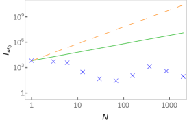
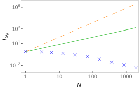
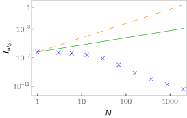
Figure 4: From left to right: Global QFI for the ZZXX model for $\omega_{0}$ for weak, medium, and strong interactions ($\delta=100$, $1$, $\delta=0.001$, and $\varepsilon=1$). Blue X-symbols: exact global QFI for $\omega_{0}$. The dashed orange (resp. green continuous) lines represent $f(N)\propto N^{2}$ (resp. $N$). Same state as in Fig.3.

III.2 Local QFI and local quantum bus observable

As we have seen in the last section, the global QFI indicates that HL scaling can be observed with a Hamiltonian of the form (2) and an initial product state. We now investigate whether it is enough for achieving the HL to measure the quantum bus. To this end, we calculate the QFI of the reduced density matrix of the quantum bus, as well as the uncertainties of the parameter estimates based on a specific observable $A$ of the quantum bus. We do not investigate further the estimation of $\omega_{0}$ as already the global QFI shows that the sensitivity cannot be improved by coupling to additional qubits.

III.2.1 Estimation of $x$

The behavior of $\delta_{x}^{A^{(0)}}$ was analyzed in second order perturbation theory in Braun11 . Within its range of validity, HL scaling was found under the condition of a noiseless observable of the quantum bus that remains noiseless without interaction with the probes. Here we relax the conditions and give a more general form in the appendix, eqs.(40,41) together with (23). Fig.5 shows HL scaling of the sensitivity for weak interactions ($\varepsilon=0.001$) for $N\lesssim 500$ and the measurement of the quantum bus $A^{(0)}=(X^{(0)}+Z^{(0)})/2)$. The perturbative result for $(\delta_{x}^{A^{(0)}})^{-2}$ agrees perfectly well with the exact numerical result in this regime. We also see that the local QFI provides an upper bound to $(\delta_{x}^{A^{(0)}})^{-2}$. However, the local QFI is rather small in the range of $N$ accessible to exact numerical evaluation, such that at least for these values of $N$ the observed HL scaling is not of much use. For larger $\varepsilon$, PT1 quickly breaks down, as is shown in Fig.5 for medium and strong interactions: For $\varepsilon=0.1$ the break down occurs at $N\simeq 10$, compatible with $N\varepsilon\simeq 10$. For $\varepsilon=100$, PT1 is already invalid in the sense that the QFI becomes negative at $N=1$ and we do not plot it. Moreover, the exact numerical values both for $1/\delta_{x}^{A^{(0)}}$ and $I_{x}^{(0)}$ show that for strong and medium interactions the achievable sensitivity through the measurement of the quantum bus alone deteriorates with increasing $N$ for large enough $N$.

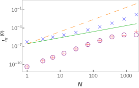
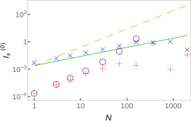
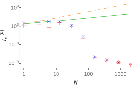
Figure 5: Local QFI and inverse squared uncertainties of $x$ based on the local observable $A^{(0)}=(X^{(0)}+Z^{(0)})/2)$ for the ZZXX model for weak, medium, and strong interactions, $\varepsilon=0.001,\,\,\,0.1$, $\varepsilon=100$, and $\delta=1$ from left to right; Blue X-symbols: exact numerical result for $I_{x}^{(0)}$. Purple circles: perturbative solution for $(\delta_{x}^{A^{(0)}})^{-2}$. Red crosses: exact solution for $(\delta_{x}^{A^{(0)}})^{-2}$. The dashed orange (resp. green continuous) lines represent $f(N)\propto N^{2}$ (resp. $N$). Same state as in Fig.3.

III.2.2 Estimation of $\omega_{1}$

A perturbative result for $\delta_{\omega_{1}}^{A^{(0)}}$ could be obtained in the case $\left[A^{(0)},R_{\nu}\right]=0$, $\left[H_{R},R_{\nu}\right]=0,\forall\nu$, and $\left[R_{\nu},R_{\mu}\right]=0,\forall\nu,\mu$. The first condition avoids that $A^{(0)}$ in the interaction picture acts non-trivially in the full Hilbert space. The second and third conditions avoid that $H_{0}$ in the interaction picture acts non-trivially in the full Hilbert space. However, all three assumptions together lead to a diverging $\delta_{\omega_{1}}^{A^{(0)}}$, as they imply $\partial_{\omega_{1}}\langle A^{(0)}\rangle=0$. Numerically we can explore a more general case where these conditions are relaxed. The results are shown in Fig. 6. For strong and medium interaction ($\delta=0.001$ and $\delta=1$), while the global QFI shows HL scaling, the local QFI goes to zero, leading to the impossibility to estimate $\omega_{1}$ by a local measurement. For weak interactions ($\delta=100$), the local QFI shows neither clear HL nor SQL scaling. Nevertheless, the SQL behavior of the global QFI sets an upper bound on the local QFI.

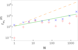
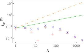
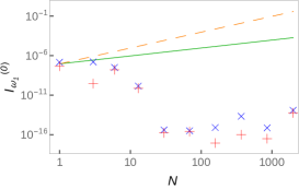
Figure 6: Local QFI and inverse squared uncertainties of $\omega_{1}$ based on the local observable $A^{(0)}=(X^{(0)}+Z^{(0)})/2$ for the ZZXX model for weak, medium, and strong interactions, $\delta=100,\,\,\,1$, $\delta=0.001$, and $\varepsilon=1$ from left to right. Blue X-symbols: exact numerical result for $I_{x}^{(0)}$. Purple circles: perturbative result for $(\delta_{x}^{A^{(0)}})^{-2}$. Red crosses: exact result for $(\delta_{x}^{A^{(0)}})^{-2}$. The dashed orange (resp. green continuous) lines represent $f(N)\propto N^{2}$ (resp. $N$). The saturation at $\leavevmode\nobreak\ 10^{-16}$ reached in the right plot corresponds to the numerical precision. Same state as in Fig.3.

III.3 Exact results for the ZZZZ model

III.3.1 Pure product state

In order to corroborate the above results we calculated the QFI for the different parameters and $\delta_{x}^{A^{(0)}}$, $I_{x}^{(0)}$, and $I_{\omega_{1}}^{(0)}$ exactly for the ZZZZ model. The expressions of the global QFI for the initial state (7) are given by

$$I_{x} = N^{2}t^{2}\varepsilon^{2}\cos^{2}(2\alpha)\sin^{2}(2\beta)+Nt^{2}\varepsilon^{2}\sin^{2}(2\alpha)\;$$ (27)

$$I_{\omega_{1}} = N\delta^{2}t^{2}\sin^{2}(2\alpha)$$ (28)

$$I_{\omega_{0}} = \delta^{2}t^{2}\sin^{2}(2\beta)\,.$$ (29)

$I_{x}$ clearly shows HL scaling as long as $\cos(2\alpha)\sin(2\beta)\neq 0$, while $\omega_{1}$ can only be measured with a sensitivity that scales as the SQL. The best possible estimation of $\omega_{0}$ does not profit from the quantum probes at all as $I_{\omega_{0}}$ is independent of $N$ and as for the ZZXX model we do not investigate it any further. All global QFIs show a scaling $\propto t^{2}$, demonstrating that the sensitivity per square root of Hertz can still be improved by measuring for longer times, in contrast to the typical time dependence of classical averaging.

The general results for the local quantities are cumbersome with the exception of $I_{\omega_{1}}^{(0)}$ which vanishes for all initial states (6) as the reduced density matrix of the quantum bus does not depend on $\omega_{1}$, see eq.(44) in the Appendix. For the estimation of $x$ we give the reduced density matrix and the uncertainty obtained via a measurement of $X^{(0)}$ in the appendix. Here, we provide results for two specific initial states. The most favorable case for the estimation of $x$, $\alpha=0$, $\beta=\pi/4$, i.e.

$$|\,\psi_{0}\,\rangle=|\,0\,\rangle^{\otimes N}\otimes\left(|\,0\,\rangle+|\,1\,\rangle\right)/\sqrt{2}\;,$$ (30)

leads to the global QFI $I_{x}=N^{2}\varepsilon^{2}t^{2}$. For the local QFI we have $I_{x}^{(0)}=N^{2}\varepsilon^{2}t^{2}$. We notice that $I_{x}=I_{x}^{(0)}$, i.e. restricting ourselves to a measurement of the quantum bus does not affect the best possible sensitivity for a estimation of $x$, and that precision follows HL scaling. Moreover, one can easily show that the corresponding QCR bound is reachable by measuring $X^{(0)}$.

Now consider the initial state with $\alpha=\pi/4$ and $\beta=\pi/4$, and $\phi=\varphi=0$, i.e.

$$|\,\psi_{0}\,\rangle=\left(|\,0\,\rangle+|\,1\,\rangle\right)^{\otimes N}\otimes\left(|\,0\,\rangle+|\,1\,\rangle\right)/2^{(N+1)/2}\;.$$ (31)

This is the worst pure state for measuring $x$. We obtain

$$I_{x}=Nt^{2}\varepsilon^{2}\;,$$ (32)

for the global QFI, i.e. SQL scaling, and

$$I_{x}^{(0)}=\frac{N^{2}t^{2}\varepsilon^{2}\tan^{2}(\varepsilon tx)}{\cos(\varepsilon tx)^{-2N}-1}.$$ (33)

for the QFI of the quantum bus. For $\varepsilon tx=\pi/2$ the QFI vanishes, which can be understood from the fact that the reduced density matrix does not depend on $x$. For the uncertainty of $x$ based on the measurement of $X^{(0)}$, we find the exact result

$$\left(\delta_{x,\text{exact}}^{X^{(0)}}\right)^{-2}=\frac{N^{2}t^{2}\varepsilon^{2}\tan^{2}(\varepsilon tx)}{\cos(\varepsilon tx)^{-2N}\cos(\delta\omega_{0}t)^{-2}-1}\,.$$ (34)

This shows that for the initial state (31), both the local QFI (33) and $(\delta_{x,\text{exact}}^{X^{(0)}})^{-2}$ decay exponentially with $N$ for sufficiently large $N$, i.e. this state is not suited for coherent averaging if we can only measure the quantum bus.

It is instructive to use PT1 for calculating $\delta_{x,\text{exact}}^{X^{(0)}}$, which leads to

$$(\delta_{x,\text{pert}}^{X^{(0)}})^{-2}=\frac{N^{2}t^{4}\varepsilon^{4}x^{2}}{Nt^{2}x^{2}\varepsilon^{2}+\tan^{2}(\delta\omega_{0}t)}\;.$$ (35)

If we expand $I_{x}^{(0)}$ in powers of $\varepsilon$, we find $I_{x}^{(0)}=Nt^{2}\varepsilon^{2}+\mathcal{O}(\varepsilon^{4})$. The exact result for $(\delta_{x,\text{exact}}^{X^{(0)}})^{-2}$ reflects the behavior of $I_{x}^{(0)}$, whereas the perturbative version, $(\delta_{x,\text{pert}}^{X^{(0)}})^{-2}$, predicts a completely different result, namely a scaling $\propto N$ for large $N$. If one stays in the range of validity of PT1, one does not notice that the uncertainty diverges.

Therefore, for the initial state (31), the validity of the perturbative expressions for the uncertainty of an observable of the quantum bus and the local QFI does break down outside the range of validity of PT1, in contrast to the global QFI, where the perturbative expression still predicts the correct scaling behavior and only differs in the prefactor from the exact result. The decaying local QFI shows that the coherent averaging scheme does not allow one to reach HL scaling for the estimation of $x$ through a measurement of the quantum bus only.

In order to find out how generic the decaying local QFI is for different initial states, we investigated the dependence of the scaling on $N$ on the angle $\alpha$ that defines the state of the probes, eq.(7). We keep $\beta=\pi/4$, $\phi=\varphi=0$. Figure 7 shows the local QFI for $x$ as a function of $\alpha$ and $N$. We see that when increasing $\alpha$ from zero, the QFI starts to decrease with $N$ for $N$ larger than some bound $N_{0}(\alpha)$, like in the case just studied ($\alpha=\pi/4$). The figure also indicates that with increasing $N$ the range of $\alpha$ leading to a non–decreasing QFI is reduced more and more. This shows that over an ensemble of initial states, a local QFI for the estimation of $x$ that decreases with $N$ is the norm, and the HL scaling for the optimal state an exception.

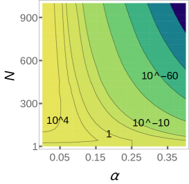
Figure 7: Local QFI for the ZZZZ model for $x$ as a function of $\alpha$ and $N$, with $\varepsilon=\delta=1$, $t=1$, $x=1$, $\omega_{0}=1$, $\omega_{1}=1$, $\beta=\pi/4$, $\phi=0$, $\varphi=0$. The contours are at $I_{x}^{(0)}=\{10^{4},10^{2},1,10^{-5},10^{-10},10^{-30},10^{-60},10^{-100},10^{-150}\}$.

III.3.2 Thermal state for the probes

In order to answer the question how a lack of purity of the initial state affects our results, we take the $N$ probes in a thermal state

$$\rho_{\text{th}}=\frac{1}{Z}\begin{pmatrix}{\rm e}\,^{-\beta_{\text{th}}\omega_{1}}&0\\ 0&{\rm e}\,^{\beta_{\text{th}}\omega_{1}}\end{pmatrix}$$ (36)

with $Z={\rm e}\,^{-\beta_{\text{th}}\omega_{1}}+{\rm e}\,^{+\beta_{\text{th}}\omega_{1}}$, $\beta_{\text{th}}=1/(k_{B}T)$, where $T$ is the temperature and $k_{B}$ the Boltzmann constant. The quantum bus is in a pure state $|\,\psi_{\text{bus}}\,\rangle=\cos(\beta)|\,0\,\rangle+\sin(\beta){\rm e}\,^{\mathrm{i}\varphi}|\,1\,\rangle$, and the new initial state is the mixed product state

$$\rho_{0}=\rho_{\text{th}}^{\otimes N}\otimes|\,\psi_{\text{bus}}\,\rangle\langle\,\psi_{\text{bus}}\,|.$$ (37)

This resembles the DQC1 protocol in quantum information processing that starts with all qubits but one in a fully mixed state, but which still allows one to solve a certain task more efficiently than with a classical computer (the “power of one qubit”) knill_power_1998 ; lanyon_experimental_2008 .

The exact results for the global QFI read

$$I_{x}=\sin^{2}(2\beta)\varepsilon^{2}t^{2}(N^{2}\tanh^{2}(\beta_{\text{th}}\omega_{1})+N(1-\tanh^{2}(\beta_{\text{th}}\omega_{1})))$$ (38)

$$I_{\omega_{1}}=N\beta_{\text{th}}^{2}(1-\tanh^{2}(\beta_{\text{th}}\omega_{1})),\text{ and }$$

$$I_{\omega_{0}}=\delta^{2}t^{2}\sin^{2}(2\beta).$$

This shows that it is possible to reach the HL scaling for the estimation of $x$ using thermal states of the probes, even though the prefactor of the $N^{2}$ term becomes small for large temperatures ($\beta_{\text{th}}\omega_{1}\ll 1$). The level spacing of the probes can only be estimated with a sensitivity scaling as the SQL, and the thermal probes are entirely useless for improving the estimation of the level spacing of the quantum bus.

Remarkably, the reduced density matrix has the same form as the one for the pure product state (6) when setting

$$\cos^{2}(\alpha)={\rm e}\,^{-\beta_{\text{th}}\omega_{1}}/Z\;\;\text{ and }\;\sin^{2}(\alpha)^{2}={\rm e}\,^{\beta_{\text{th}}\omega_{1}}/Z.$$ (39)

This implies that for any pure product state (6) there exists a thermal state of the probes with the same $I_{x}^{(0)}$ and hence the same best possible sensitivity of estimating $x$ by measuring the quantum bus. For locally estimating $\omega_{1}$, a thermal state of the probes is advantageous compared to the pure state (30) where the corresponding local QFI vanishes. The thermal state introduces a dependence on $\omega_{1}$ through the initial state that is absent for the pure states considered. If also the quantum bus is in a thermal state initially, the interaction strength cannot be measured in the ZZZZ model.

IV Summary

In summary, we have examined in detail a coherent averaging scheme for its usefulness of Heisenberg-limited precision measurements. In the scheme, $N$ probes that are initially in a product state, interact with a quantum bus and one measures the latter or the entire system. Combining analytical results from perturbation theory and an exactly solvable dephasing model with numerical results, we have shown that this setup allows one to measure the interaction strength and the level spacing of the probes with HL sensitivity if one has access to the entire system. Strong interactions favor better sensitivities in this case. If one has only access to the quantum bus, the results depend on the initial state, but HL sensitivity is achievable only for the interaction strength and a small set of initial states.

Remarkably, for measuring the interaction strength in the exactly solvable ZZZZ model, there is a mapping of the local quantum Fisher information for thermal states of the probes to the one for pure states. Globally HL sensitivity for estimating the interaction strength can be achieved with thermal probes at any finite temperature, as long as the quantum bus can be brought into an initially pure state. The sensitivity of measurements of the level spacing of the quantum bus cannot be improved by coupling it to many probes, even with access to the entire system, and in fact deteriorates with an increasing number of probes. Altogether, our investigations have led to a broader and more detailed view of the usefulness of the coherent averaging scheme and may open the path to experimental implementation.

V Appendices

V.1 Uncertainty of a local observable

If one relaxes the condition used in Braun11 , namely that $A|\,\xi\,\rangle=a_{\xi}|\,\xi\,\rangle$ and $[A^{(0)},H_{R}]=0$, one finds for the variance of the observable $A^{(0)}$

$$\text{Var}(A^{(0)})=\langle\,A^{2}\,\rangle-\langle\,A\,\rangle^{2}+\mathrm{i}\varepsilon\int_{0}^{t}dt_{1}N\langle\,S_{\nu}(t_{1})\,\rangle\langle\,[R_{\nu}(t_{1}),B]\,\rangle$$

$$+\varepsilon^{2}\int_{0}^{t}\int_{0}^{t_{1}}dt_{1}dt_{2}\left\{(N(N-1)\langle\,S_{\nu}(t_{1})\,\rangle\langle\,S_{\mu}(t_{2})\,\rangle\right.$$

$$+N\langle\,S_{\nu}(t_{1})S_{\mu}(t_{2})\,\rangle)\langle\,[R_{\nu}(t_{1}),B]R_{\mu}(t_{2})\,\rangle$$

$$+(N(N-1)\langle\,S_{\nu}(t_{1})\,\rangle\langle\,S_{\mu}(t_{2})\,\rangle+N\langle\,S_{\mu}(t_{2})S_{\nu}(t_{1})\,\rangle)$$

$$\left.\langle\,R_{\mu}(t_{2})[B,R_{\nu}(t_{1})]\,\rangle\right\}+\varepsilon^{2}\int_{0}^{t}\int_{0}^{t}dt_{1}dt_{2}N^{2}\langle\,S_{\nu}(t_{1})\,\rangle$$

$$\langle\,S_{\mu}(t_{2})\,\rangle\langle\,[R_{\nu}(t_{1}),A]\,\rangle\langle\,[R_{\mu}(t_{2}),A]\,\rangle$$ (40)

where $B=A^{2}-2\langle\,A\,\rangle A$, the expectation values for $A$, $B$, and $R_{\mu}(t)$ are taken with respect to $|\,\xi\,\rangle$, and the expectation value for $S_{\mu}(t)\equiv S_{\mu}(x,t)$ is with respect to $|\,\varphi\,\rangle$. The derivative of the mean value of $A^{(0)}$ is given by

$$\frac{\partial}{\partial\theta}\langle A^{(0)}\rangle=\frac{\partial}{\partial\theta}\left(\mathrm{i}\varepsilon\int_{0}^{t}dt_{1}N\langle\,S_{\nu}(t_{1})\,\rangle\langle\,[R_{\nu}(t_{1}),A]\,\rangle\right.$$ (41)

$$+\varepsilon^{2}\int_{0}^{t}\int_{0}^{t_{1}}dt_{1}dt_{2}\left\{(N(N-1)\langle\,S_{\nu}(t_{1})\,\rangle\langle\,S_{\mu}(t_{2})\,\rangle\right.$$

$$+N\langle\,S_{\nu}(t_{1})S_{\mu}(t_{2})\,\rangle)\langle\,[R_{\nu}(t_{1}),A]R_{\mu}(t_{2})\,\rangle$$

$$+(N(N-1)\langle\,S_{\nu}(t_{1})\,\rangle\langle\,S_{\mu}(t_{2})\,\rangle+N\langle\,S_{\mu}(t_{2})S_{\nu}(t_{1})\,\rangle)$$

$$\left.\langle\,R_{\mu}(t_{2})[A,R_{\nu}(t_{1})]\,\rangle\right\}\Big{)}\;.$$

From these two quantities we obtain $\delta_{x}^{A^{(0)}}$ according to eq.(23).

V.2 Local analysis of ZZZZ

The reduced density matrix $\rho^{(0)}$ for the ZZZZ model starting in a pure product state (7) has the matrix elements

$$\rho^{(0)}_{00} = \cos^{2}(\beta)$$ (42)

$$\rho^{(0)}_{11} = \sin^{2}(\beta)$$ (43)

$$\rho^{(0)}_{01} = \frac{1}{2}\sin(2\beta){\rm e}\,^{-\mathrm{i}(\varphi+\delta\omega_{0}t)}(\cos^{2}(\alpha){\rm e}\,^{-\mathrm{i}\varepsilon xt}+\sin(\alpha)^{2}{\rm e}\,^{\mathrm{i}\varepsilon xt})^{N}\,,$$ (44)

from which one can easily compute the local QFI.

The relative uncertainty for $x$ using a measurement $X^{(0)}$ is:

$$(\delta_{x,\text{pert}}^{X^{(0)}})^{2}=\frac{1-\left(\sin(2\beta)\sum_{m=-N/2}^{N/2}\binom{N}{m-N/2}\cos(\alpha)^{N+2m}\sin(\alpha)^{N-2m}\cos(\delta\omega_{0}t+\varphi+2\varepsilon xtm)\right)^{2}}{\left|2\varepsilon t\sin(2\beta)\sum_{m=-N/2}^{N/2}\binom{N}{m-N/2}m\cos(\alpha)^{N+2m}\sin(\alpha)^{N-2m}\sin(\delta\omega_{0}t+\varphi+2\varepsilon xtm)\right|^{2}}\;.$$ (45)

References

- (1) Giovannetti, V., Loyd, S., & Maccone, L., Quantum-Enhanced Measurements: Beating the Standard Quantum Limit, Science 306, 1330–1336 (2004).
- (2) Leibfried, D. et al., Creation of a six-atom ’Schrodinger cat’ state, Nature 438, 639–642 (2005).
- (3) Nagata, T., Okamoto, R., O’Brien, J. L., & Takeuchi, K. S. S., Beating the Standard Quantum Limit with Four-Entangled Photons, Science 316, 726–729 (2007).
- (4) Higgins, B. L., Berry, D. W., Bartlett, S. D., Wiseman, H. M., & Pryde, G. J., Entanglement-free Heisenberg-limited phase estimation, Nature 450, 393–396 (2007).
- (5) Pinel, O. et al., Ultimate sensitivity of precision measurements with intense Gaussian quantum light: A multimodal approach, Phys. Rev. A 85, 010101 (2012).
- (6) Braun, D. & Martin, J., Collectively enhanced quantum measurements at the Heisenberg limit, eprint arXiv:1005.4443.
- (7) Braun, D. & Martin, J., Heisenberg-limited sensitivity with decoherence-enhanced measurements, Nat. Commun. 2, 223 (2011).
- (8) Braun, D. & Popescu, S., Coherently enhanced measurements in classical mechanics, Quantum Measurements and Quantum Metrology 2 (2014).
- (9) Luis, A., Quantum limits, nonseparable transformations, and nonlinear optics, Phys. Rev. A 76, 035801 (2007).
- (10) Napolitano, M. et al., Interaction-based quantum metrology showing scaling beyond the Heisenberg limit, Nature 471, 486–489 (2011).
- (11) Marzolino, U. & Braun, D., Precision measurements of temperature and chemical potential of quantum gases, Phys. Rev. A 88, 063609 (2013).
- (12) Arshed, N., Toor, A. H., & Lidar, D. A., Channel capacities of an exactly solvable spin-star system, Phys. Rev. A 81, 062353 (2010).
- (13) Ferraro, E., Napoli, A., & Messina, A., Entanglement dynamics in a spin star system, in 11th International Conference on Transparent Optical Networks, 2009. ICTON ’09, 1–1 (2009).
- (14) Hamdouni, Y., An exactly solvable model for the dynamics of two spin-\frac{1}{2} particles embedded in separate spin star environments, J. Phys. A: Math. Theor. 42, 315301 (2009).
- (15) Rao, C. R., Information and the accuracy attainable in the estimation of statistical parameters, Bull. Calcutta Math. Soc. 37, 81–91 (1945).
- (16) Cramér, H., Mathematical Methods of Statistics (Princeton University Press, Princeton, NJ, 1946).
- (17) Peres, A., Quantum Theory: Concepts and Methods (Kluwer Academic Publishers, Dordrecht, 1993).
- (18) Braun, D., Jian, P., Pinel, O., & Treps, N., Precision measurements with photon-subtracted or photon-added Gaussian states, Phys. Rev. A 90, 013821 (2014).
- (19) Paris, M. G. A., Quantum estimation for quantum technology, International Journal of Quantum Information 7, 125 (2009).
- (20) Braunstein, S. L. & Caves, C. M., Statistical distance and the geometry of quantum states, Phys. Rev. Lett. 72, 3439–3443 (1994).
- (21) Braunstein, S. L., Caves, C. M., & Milburn, G. J., Generalized Uncertainty Relations: Theory, Examples, and Lorentz Invariance, Annals of Physics 247, 135–173 (1996).
- (22) Bengtsson, I. & Życzkowski, K., Geometry of quantum states: an introduction to quantum entanglement (Cambride University Press, 2006).
- (23) Escher, B. M., de Matos Filho, R. L., & Davidovich, L., General framework for estimating the ultimate precision limit in noisy quantum-enhanced metrology, Nat. Phys. 7, 406–411 (2011).
- (24) Kołodyński, J. & Demkowicz-Dobrzański, R., Phase estimation without a priori phase knowledge in the presence of loss, Phys. Rev. A 82, 053804 (2010).
- (25) Kay, S. M., Fundamentals of Statistical Processing, Volume I: Estimation Theory (Prentice Hall, Englewood Cliffs, N.J, 1993), new. edn.
- (26) Knill, E. & Laflamme, R., Power of One Bit of Quantum Information, Phys. Rev. Lett. 81, 5672–5675 (1998).
- (27) Lanyon, B. P., Barbieri, M., Almeida, M. P., & White, A. G., Experimental Quantum Computing without Entanglement, Phys. Rev. Lett. 101, 200501 (2008).