A Sharing- and Competition-Aware Framework
for Cellular Network Evolution Planning

Abstract

Mobile network operators are facing the difficult task of significantly increasing capacity to meet projected demand while keeping CAPEX and OPEX down. We argue that infrastructure sharing is a key consideration in operators’ planning of the evolution of their networks, and that such planning can be viewed as a stage in the cognitive cycle. In this paper, we present a framework to model this planning process while taking into account both the ability to share resources and the constraints imposed by competition regulation (the latter quantified using the Herfindahl index). Using real-world demand and deployment data, we find that the ability to share infrastructure essentially moves capacity from rural, sparsely populated areas (where some of the current infrastructure can be decommissioned) to urban ones (where most of the next-generation base stations would be deployed), with significant increases in resource efficiency. Tight competition regulation somewhat limits the ability to share but does not entirely jeopardize those gains, while having the secondary effect of encouraging the wider deployment of next-generation technologies.

1 Introduction

With cellular coverage reaching virtually every human being on the planet, the challenge now lies in evolving the existing infrastructure to cope with foreseen explosion in the demand for capacity [1]. Evolution will mean different things at different locations: some parts of the infrastructure will be replaced with new-generation equipment, e.g., LTE and its successors; others will be upgraded for the purpose of enhancing capacity, e.g., by increasing sectorization; finally, underutilized base stations will be decommissioned, possibly permanently.

The yellow, solid curve in Fig. 1 represents the network load and its familiar predicted almost-exponential growth from the current level in $A$ to a future one in $\Omega$. Dashed lines represent possible evolutions of the network capacity: there is no question that capacity has to increase from its current level at point $B$ to $\Omega$, so as to serve all the demand; in this paper we investigate how and when the required changes to the network shall be performed, so as to efficiently match available capacity to demand, minimizing over-provisioning.

\psfrag{A}[1]{$B$}\psfrag{B}[1]{$A$}\psfrag{Z}[1]{$\Omega$}\includegraphics[width=195.12767pt]{concept_time}

Figure 1: The present and future evolution of cellular infrastructures. The solid yellow line represents the traffic demand, growing from its present value in $A$ to a much higher one in $\Omega$. Dashed lines represent different evolutions of network capacity. Its present value (in $B$) is higher than the current demand $A$, but lower than the future demand $\Omega$. The area between the capacity and demand curves corresponds to unused capacity (shaded in gray). Network capacity therefore has to grow from $B$ to $\Omega$ in the long term, possibly decreasing in the short term in order to reduce the amount of unused capacity.

The reason why this matters is the gray area in Fig. 1, representing unused network capacity. Providing capacity that nobody uses is a waste of bandwidth, resources and, ultimately, money; therefore, it is of paramount importance for operators to keep overprovisioning as low as possible. Furthermore, Fig. 1 refers to the network as a whole; the relative positions of points $A,B,\Omega$ can be different in different parts of the topology [2]. Extreme cases include some sparsely populated rural areas, where the current capacity may exceed not only the current but also the future demand, i.e., $B>\Omega$, and very dense urban areas, which may have $A\approx B$.

Ideally, operators would like their capacity to instantly fall from $B$ to $A$ at all locations, and would achieve this by decommissioning as many base stations as possible. Then, they would follow the demand curve all the way to $\Omega$, by updating their infrastructure as the load increases, always keeping the unutilized capacity (i.e., the gray area in Fig. 1) to zero.

Such an idealized view conflicts with the reality that making any change to a network, be it deploying new base stations, updating or decommissioning existing ones, requires equipment, work-power, and funds – all resources that are scarce, and whose usage must be carefully planned. The number of such changes operators can perform in a given time, e.g., a month, is typically limited, and such a limit directly impacts the speed at which network capacity can go down or up, hence the gray area in Fig. 1.

Our first goal is then to study the efficient evolution of the cellular infrastructure in light of the limited budget of possible network changes. The input to our problem consists of the current set of base stations, the (projected, possibly based on real-world measurements and topologies) future demand and a limited change rate at which we can update, replace or decommission base stations. This change rate reflects the operators’ limitations in terms of how they are able to reshape their own network. The output we seek is a list of the changes to perform to the network, and the time at which to enact each of them. The overall objective is to keep unused capacity, i.e., the gray area in Fig. 1, at a minimum.

In studying this problem we account for two important real-world issues: network sharing and competition regulation. Both are widely studied in the literature, but their impact on the evolution of cellular networks has received relatively little attention so far.

Active network sharing [3, 4] refers to roaming-like agreements between mobile operators, where users of each operator are served through both networks indifferently. It is emerging as a promising way to achieve cost savings and enhanced performance; indeed, running their networks in such a shared fashion makes it easier for operators to identify underutilized base stations to decommission, as well as making the most out of updated, more highly performing infrastructure.

Competition regulation, on the other hand, has the potential to limit the operators’ ability to reduce unused capacity. Unused capacity is, from the viewpoint of market regulators, capacity that can be sold to new market players, typically virtual operators, which would increase the level of competition. It is entirely plausible, therefore, that existing operators be mandated to keep a certain amount of unused spectrum in at least some part of the topology; indeed, a similar condition was recently imposed to O2 and Three when they merged their Irish branches [5]. Studying how sharing and competition regulation shape the evolution of networks is thus an important contribution of this paper.

The algorithms we present are most readily separated into three phases: meeting demand, regulation compliance, and cost reduction. Each of the phases occur in series to update the network of an operator in order to provide service to increasing demand while minimising over-provisioning.

In our view, each individual phase conforms to a instantiation of the cognition loop. Specifically, each phase of the operation has observation, decision, and action steps. During observation the current situation is assessed in terms of the current network, the current demand, the already planned updates, and the expected demand. Decision involves the application of this situational awareness to some optimization. Actions take the form of changes to the schedule of network updates. Note that none of the phases explicitly involves learning. Rather, each phase implements cognition as optimization based on situational awareness of network and subscriber state.

Furthermore, the collection of all the phases together provides a more nuanced form of cognition. This cognition uses understanding of current network infrastructure to plan future deployments based on the input of expected demand and regulatory policy. As a unit the three phases of our algorithms periodically receive an observation of projected demand, whereupon a plan for network updates is constructed. This plan is then used to decide which base station updates should be applied to the current infrastructure and the action of making these adjustments is taken.

The remainder of this paper is organized as follows. We present our system model in Sec. 2. In Sec. 3, we state and solve the problem of scheduling the changes to our network, and discuss its computational complexity and performance in Sec. 4. Sec. 5 presents our reference scenario, which we use to obtain the results we present in Sec. 6. Finally, after a related work review in Sec. 7, Sec. 8 concludes the paper.

2 System model

Our system model revolves around two main elements: base stations and subscriber clusters.

Model elements Base stations $b\in\mathcal{B}$ are elements of the infrastructure with a certain position, capacity, and coverage area. Subscriber clusters $c\in\mathcal{C}$ can correspond to one or more actual users, which can be viewed as co-located. They have a known position and traffic demand. We also have operators $o\in\mathcal{O}$, and time periods $k\in\mathcal{K}=\{1\dots K\}$.

Base station type Base stations are not all equal. They can differ in technology, e.g., GSM, 3G, or LTE; furthermore, even base stations with the same technology differ in such aspects as frequency of operation and sectorization. Indeed, upgrading a cellular network essentially means changing their type, e.g., from 3G to LTE. Even disabling a base station can be seen as changing its type to “off”.

In our model, possible base station types are collected in set $\mathcal{T}$, and every base station $b\in\mathcal{B}$ has a type $T(b)\in\mathcal{T}$. Decommissioned base stations have the special type $t_{\emptyset}$. The type of a base station determines its coverage and performance, as shown next, as well as its associated cost.

Coverage and demand Our coverage information comes in the form of binary flags $\gamma(b,c,t)\in\{0,1\}$, expressing whether base station $b$ covers subscriber cluster $c$ if $b$ is of type $t$, i.e., if $T(b)=t$. Notice how these values do not depend upon time. We indicate with $\delta(b,c)\in\mathds{R}_{+}$ the distance between base stations and subscriber clusters.

Requested and served traffic For each subscriber cluster $c$, operator $o$ and time period $k$, we know the traffic demand $\tau(c,k,o)$ from users of operator $o$ in cluster $c$ at period $k$. To streamline the notation, we will often write $\tau(c,k)=\sum_{o\in\mathcal{O}}\tau(c,k,o)$.

We also indicate with $\sigma(b,c,k,o,t)$ the traffic demand that can be met by base station $b$, of type $t$, when servicing users of operator $o$ in cluster $c$ at period $k$. Similarly to $\sigma$, we will often drop indices to streamline the notation, and write, e.g., $\sigma(c,k,o)=\sum_{b\in\mathcal{B}}\sum_{t\in\mathcal{T}}\sigma(b,c,k,o,t)$.

\psfrag{b}[c][m]{Base}\psfrag{s}[c][m]{station}\psfrag{b1}[c][m]{$b_{1}$}\psfrag{b2}[c][m]{$b_{2}$}\psfrag{b3}[c][m]{$b_{3}$}\psfrag{k1}[c][m]{$k=1$}\psfrag{k2}[c][m]{$k=2$}\psfrag{k3}[c][m]{$k=3$}\psfrag{k4}[c][m]{$k=4$}\psfrag{k5}[c][m]{$k=5$}\psfrag{u12}[c][m]{\footnotesize{$x(b_{1},2,$}}\psfrag{u14}[c][m]{\footnotesize{$x(b_{1},4,$}}\psfrag{u21}[c][m]{\footnotesize{$x(b_{2},1,$}}\psfrag{w33}[c][m]{\footnotesize{$x(b_{3},3,$}}\psfrag{x1}[c][m]{\footnotesize{$t_{2})=1$}}\psfrag{x2}[c][m]{\footnotesize{$t_{3})=1$}}\psfrag{x3}[c][m]{\footnotesize{$t_{2})=1$}}\psfrag{x4}[c][m]{\footnotesize{$t_{\emptyset}$)=1}}\includegraphics[width=195.12767pt]{table}

Figure 2: An example schedule, with $|\mathcal{B}|=3$ base stations and $|\mathcal{K}|=4$ time periods. The maximum change rate is $N=1$, i.e., we can make at most one change (updating or disabling a base station) per time period. Let us assume $\mathcal{T}=\left\{t_{\emptyset},t_{1},t_{2},t_{3}\right\}$, with $t_{1}\dots t_{3}$ having increasing capacity and the same coverage. All base stations start with type $t_{1}$. Green arrows mark the periods at which base stations need to be updated due to an increased load, i.e., because $\tau>\sigma$; some stations, such as $b_{1}$, may need more than one update. We update $b_{1}$ twice, from $t_{1}$ to $t_{2}$ and then to $t_{3}$, setting $x(b_{1},2,t_{2})=x(b_{1},4,t_{3})=1$. Base station $b_{2}$ needs an update within $k=2$; However, we cannot set $x(b_{2},2,t_{2})=1$, because doing so would violate constraint Eq. (1). This forces us to anticipate the update to $k=1$, i.e., set $x(b_{2},1,t_{2})=1$. Similarly, the red arrow tells us that we would be able to decommission $b_{3}$ as soon as $k=1$, but the updates we already scheduled force us to delay until $k=3$, and set $x(b_{3},3,t_{\emptyset})=1$.

Cost Base stations also have an operational cost $\kappa(b,T(b))$. Such a cost is base station- and type-dependent, and models such aspects as maintenance, site rental, and energy consumption. The cost associated with decommissioned base stations is zero, i.e., $\kappa(b,t_{\emptyset})=0,\forall b\in\mathcal{B}$.

Network changes All our decisions concern network changes. At each time period $k$, we may decide to change the type of base station $b$, either to a better-performing type $t_{dest}$, in order to increase its capacity, or to $t_{\emptyset}$ to save on costs, as shown in Fig. 2. We track type changes through binary variables:

$$x(b,k,t_{dest})\in\{0,1\}.$$

Setting $x(b,k,t_{dest})=1$ means that, at time $k$, we change the type of base station $b\in\mathcal{B}$ to $t_{dest}\in\mathcal{T}$. Doing nothing, i.e., never changing $b$’s type, is represented by having $x(b,k,t)=0,\forall k,t$.

Also notice that we can change a base station’s type multiple times, i.e., it can be
that $\sum_{k\in\mathcal{K},t\in\mathcal{T}}x(b,k,t)>1$. We do not explicitly forbid changing the type to $t_{\emptyset}$ and then to some other type, i.e., first disabling and then re-enabling a base station, although it is unlikely to make sense in practice (and we never observe that behavior in our performance evaluation).

Changing the type of a base station to $t_{\emptyset}$ means reducing network capacity and saving money, i.e., going down in Fig. 1. On the contrary, moving to a better-performing type means being able to serve more traffic, hence going up in Fig. 1.

In both cases, as discussed in Sec. 1, setting more $x$-values to $1$ is linked to going up or down in Fig. 1 with a higher slope, i.e., being more effective in reducing the gap between requested and provided capacity.

What limits us is the maximum change rate $N$, defined as the maximum number of changes we can make to our network at each time period $k$. The following constraint must hold:

$$\sum_{b\in\mathcal{B},t\in\mathcal{T}}x(b,k,t)\leq N,\forall k\in\mathcal{K}.$$ (1)

Having Eq. (1) in place means two things. First and most obviously, we can take fewer actions, e.g., decommission fewer base stations. Furthermore, we may have to move some actions in time, e.g., decommission a base station later than we would like to. Both make us less effective in tracking the demand, i.e., imply a larger gray area in Fig. 1.

Time scale It is important to understand the time scale at which our model, and the algorithms described later, work. We are modeling network planning, and we are concerned with the evolution of our network over a time span of months or years. Each time period $k\in\mathcal{K}$ may correspond to several weeks, and the decisions $x(b,k,t)$ can be mapped, e.g., to equipment orders or to the schedule of infrastructure deployment teams. Decommissioning or updating a base station is substantially different from turning it on and off in order to follow daily traffic fluctuation, as envisioned in “green networking” solutions [6, 7, 8]. Indeed, as discussed later, the two solutions are orthogonal and altogether compatible.

Since networks have to be provisioned for peak loads and not average ones, the $\tau(c,k)$ values express the worst-case amount of traffic requested by subscriber cluster $c$ during the whole duration of time period $k$ – e.g., the amount of traffic (in Mbit) that users in $c$ will need served during the busiest hour of time period $k$. Such values typically come from forecasts and projections; from the viewpoint of our model, they are an input.

It is also worthwhile to observe that our network must be able to operate even if all the “worst hours” of all subscriber clusters take place at the same time. In other words, while it is possible, and indeed advisable, to operate the network so as to take advantage of the low space and traffic correlation in traffic demand [2], such an effect cannot be depended upon in the planning phase.

Assessing network performance It is important to remark that our model does not explicitly include a representation of how the served traffic $\sigma$ depends on the other parameters and variables, e.g., our decisions $x$. As we see in Fig. 3, the $\sigma$-values are obtained through an external performance assessment block. In addition to keeping our model simple, this choice affords us a higher degree of flexibility: we can interface our model with a simulation tool, or leverage any real-world data available to us, as discussed in Sec. 5.

\psfrag{A}[c][m]{{Alg.~{}\ref{alg:capacity}}}\psfrag{B}[c][m]{{Alg.~{}\ref{alg:competition}}}\psfrag{C}[c][m]{{Alg.~{}\ref{alg:disable}}}\psfrag{S}[c][m]{{Performance assessment}}\psfrag{t}[c][m]{\footnotesize{{(Simulators, real data...)}}}\psfrag{y}[l]{\footnotesize{$\sigma$}}\psfrag{z}[c]{\footnotesize{$\mathcal{C},\mathcal{B},\tau\dots$}}\psfrag{x}[r]{\footnotesize{$x$}}\includegraphics[width=195.12767pt]{simulator}

Figure 3: Assessing the performance within our model and solution concept. Network performance depends on topology, traffic demand and decisions; however, our model does not explicitly represent such a dependency. Our algorithms rely instead on an external block, represented by the cloud in the figure. Given as an input the network topology (base stations $\mathcal{B}$, subscriber clusters $\mathcal{C}$), demand $\delta$, and decisions $x$, it returns the traffic that can be served by the network, $\sigma$, as an output. The most straightforward way of implementing such a block is network simulation; however, other approaches are possible. As discussed in Sec. 5, we implement the performance assessment block leveraging real-world traces.

Competition Healthy competition within the mobile market is of constant concern to regulators, as dominance on the part of large operators can lead to market abuses. A common regulatory tool to measure the level of competition and market concentration is the Herfindahl index (HHI) [9, 10]. It is given by the sum of the squares of shares held by each operator in the market, and takes values between 0 (a multitude of operators with a zero-share) and 1 (a monopolist with a 100% share). The HHI can be used to assess concentration in different aspects of the market, e.g., overall market share, concentration in ownership of spectrum and concentration in ownership of network infrastructure.

In our scenario, we need to define a local version of HHI, specific to each subscriber cluster (as well as to each time period). Furthermore, we have to account not only for the operators currently in $\mathcal{O}$, but also for new operators that may enter the market if the conditions are favorable – typically mobile virtual operators (MVNOs). Our version of the HHI is thus given by:

$$H(c,k)=\left(\frac{\sigma(c,k)-\tau(c,k)}{\sigma(c,k)}\right)^{2}+\sum_{o\in\mathcal{O}}\left(\frac{\tau(c,k,o)}{\sigma(c,k)}\right)^{2}$$ (2)

In the denominator of Eq. (2) we always find the total capacity $\sigma(c,k)$ available to subscriber cluster $c$ at time period $k$ (recall our conventions about dropping indices). In the numerator we have the traffic of current operators in $\mathcal{O}$ in the summation, and the spare capacity, i.e., the traffic of potential new operators, in the other term.

When two operators deploy and manage their networks in a shared fashion, they behave as one from the competition viewpoint. Therefore, the set $\mathcal{O}$ shrinks, and the HHI in Eq. (2) increases. In our model, regulators require that the HHI not exceed a value $H_{\max}$ in at least a significant portion of the topology.

3 Problem formulation and solution

In this section, we address the following problem. Given the future demand $\tau(c,k,o)$, and the maximum change rate $N$, how should each operator schedule the network changes, i.e., set the $x$-variables? Operators have three goals:

Goal 1 is meeting the traffic demand, i.e., having:

$$\sigma(c,k,o)\geq\tau(c,k,o),\forall c\in\mathcal{C},k\in\mathcal{K},o\in\mathcal{O}.$$ (3)

Eq. (3) says that for all subscriber clusters $c$, time periods $k\in\mathcal{K}$ and operators $o\in\mathcal{O}$, the provided capacity $\sigma$ must equal (or exceed) the demand $\tau$.

Goal 2 is complying with existing regulation:

$$\sum_{c\in\mathcal{C}}\mathds{1}_{\left[{H(c,k)\leq H_{\max}}\right]}\geq\phi\cdot|\mathcal{C}|,\forall k\in\mathcal{K}.$$ (4)

Eq. (4) imposes that, for each time period, at least a fraction $\phi$ of demand clusters – enough for a new operator to start building its network [5, 11] – have an HHI (as defined in Eq. (2)) not exceeding the limit $H_{\max}$.

Goal 3 is to minimize costs:

$$\min\sum_{b\in\mathcal{B},k\in\mathcal{K}}\kappa(b,T(b)).$$ (5)

An obvious way to decrease the quantity in Eq. (5) is setting the type of some base stations to $t_{\emptyset}$, whose associated cost is $0$, i.e., disabling them.

Multi-objective problems, where some kind of trade-off between different goals is sought, are in general hard to formulate and harder to solve. Thankfully, in our case goals have a clear hierarchy: the first two goals must be met through as few changes to the network as possible; any remaining change can be used to pursue the third goal. Indeed, the first two goals can be treated as constraints, and the third one is the objective we seek to optimize.

3.1 Solution concept

Our aim is to exploit the hierarchy of the goals stated above, as well as their features, to devise a solution concept that addresses them in sequence.

We begin by defining a class of network changes, that we call capacity-preserving changes, as follows:

Definition 1.

Changing the type of a base station $b$ from $t_{orig}$ to $t_{dest}$ is capacity-preserving if the capacity available to each subscriber cluster does not decrease, i.e.,

$$\pi(b,t_{orig},t_{dest})=1\Leftrightarrow\sigma(b,c,t_{dest})\geq\sigma(b,c,t_{orig}),\forall c\in\mathcal{C}.$$ (6)

Intuitively, capacity-preserving network changes increase the capacity available to certain subscriber clusters, without hurting others. Increasing the number of sectors of a base station is a capacity-preserving change, as is replacing a GSM base station with an LTE-800 one, having the same coverage and a higher capacity. Replacing the same GSM base station with an LTE-2600 one is not capacity-preserving, as the new base station will have smaller coverage and some subscriber clusters, namely the ones covered by the old base station but not by the new one, will suffer a decrease in their available capacity. Similarly, changing any base station’s type to $t_{\emptyset}$ is not capacity-preserving.

We are now in the position of proving the following useful properties:

Property 1.

Both goal 1 and goal 2 can be reached through capacity-preserving changes alone, i.e., changes that comply with Eq. (6).

Proof:

See the Appendix. ∎

Property 2.

If the initial configuration satisfies goal 1, then pursuing goal 2 by scheduling further capacity-preserving changes does not compromise goal 1.

\psfrag{c1}[c][m]{\scriptsize{Capacity}}\psfrag{c2}[c][m]{\scriptsize{shortage?}}\psfrag{c3}[c][m]{\scriptsize{Competition}}\psfrag{c4}[c][m]{\scriptsize{rule breach?}}\psfrag{c01}[c][m]{\scriptsize{Coverage,}}\psfrag{c02}[c][m]{\scriptsize{capacity, and}}\psfrag{c03}[c][m]{\scriptsize{competition}}\psfrag{c04}[c][m]{\scriptsize{respected?}}\psfrag{f1}[c][m]{\scriptsize{Find subscriber}}\psfrag{f2}[c][m]{\scriptsize{clusters with}}\psfrag{f3}[c][m]{\scriptsize{problems}}\psfrag{s2}[c][m]{\scriptsize{base station}}\psfrag{s01}[c][m]{\scriptsize{Select}}\psfrag{s02}[c][m]{\scriptsize{most urgent}}\psfrag{s03}[c][m]{\scriptsize{subscriber cluster}}\psfrag{f01}[c][m]{\scriptsize{Find suitable}}\psfrag{f02}[c][m]{\scriptsize{base stations to}}\psfrag{f03}[c][m]{\scriptsize{solve the problem}}\psfrag{u01}[c][m]{\scriptsize{Update the most}}\psfrag{u02}[c][m]{\scriptsize{appropriate one as}}\psfrag{u03}[c][m]{\scriptsize{late as possible}}\psfrag{d01}[c][m]{\scriptsize{Decommission as early}}\psfrag{d02}[c][m]{\scriptsize{as possible}}\psfrag{n}[c][m]{\small{no}}\psfrag{y}[c][m]{\small{yes}}\includegraphics[width=433.62pt]{algo}

Figure 4: Our solution concept. The three phases correspond to our three objectives – meeting the traffic demand, complying with competition regulation, and reducing costs. Within each phase, we proceed in a similar way: identify the subscriber clusters that call for action, e.g., whose demand is not satisfied; identify the base stations that can be acted upon to solve the problem, i.e., whose type shall be changed, and schedule the needed action at the most appropriate time. Notice that once we are done with a phase we never come back to it, and subsequent decisions are guaranteed not to jeopardize its objective.

Exploiting these properties, we propose the solution concept shown in Fig. 4, where objectives are addressed in sequence. Specifically, we first address goal 1, and do so by scheduling capacity-preserving network changes (Property 1 guarantees that it is sufficient). Then, we schedule further capacity-preserving changes in order to reach goal 2: Property 1 again guarantees that it is possible, and Property 2 makes sure that doing so will not jeopardize goal 1. Finally, we use any remaining changes we can make to the network to pursue goal 3, as long as doing so does not conflict with goals 1 and 2. Notice that in this last step we are not restricted to capacity-preserving changes, e.g., we can decommission base stations by changing their type to $t_{\emptyset}$.

With reference to Fig. 4, we can clearly see how the three goals stated above correspond to three phases in the algorithm. Within each phase, we proceed in a similar, greedy way: identify the problems and find the most urgent one to fix; identify the possible actions and find the most appropriate one; and schedule said action at the most appropriate time.

It is worth stressing that from our viewpoint the future demand, i.e. the $\tau$-values, is but an input to our problem. In practical settings, such demand will not be known with precision, and this will call for appropriate action, e.g., considering a safety margin. Our approach, however, remains unchanged.

3.2 Individual phases

Alg. 1 summarizes the steps we take in the first phase, where our objective is making sure that the traffic demand is met at all times and for all subscriber clusters. It works unmodified with and without network sharing: if there is no sharing, each operator will run Alg. 1 independently, feeding it its own network and its own load. If operators are performing their updates in a shared fashion, then Alg. 1 will be run only once, on the joint network and the total load.

1:$\mathcal{B},\mathcal{C},\mathcal{K},\tau$

2:while true do

3:     $\sigma\leftarrow\texttt{assess}(x,\delta,\gamma,\tau)$

4:     $\texttt{problems}\leftarrow\{(c,k)\in\mathcal{C}\times\mathcal{K}:\sigma(c,k)<\tau(c,k)\}$

5:     if $\texttt{problems}\equiv\emptyset$ then

6:         break      

7:     $c^{\star},k^{\star}\leftarrow\arg\min_{(c,k)\in\texttt{problems}}k$

8:     $\texttt{actions}\leftarrow\{(b,t)\in\mathcal{B}\times\mathcal{T}:\gamma(b,c^{\star},t)=1\wedge\pi(b,T(b),t)=1\}$

9:     $b^{\star}\leftarrow\arg\min_{(b,t)\in\texttt{actions}}\delta(b,c^{\star})$

10:     $t^{\star}\leftarrow\arg\min_{(b,t)\in\texttt{actions}\colon\sigma(c,k,t)\geq\tau(c,k)}\kappa(b,t)$

11:     $\hat{k}\leftarrow\arg\max_{h=0}^{k^{\star}}\{h:\sum_{b\in\mathcal{B},t\in\mathcal{T}}x(b,k,t)<N\}$

12:     $x(b^{\star},\hat{k},t^{\star})\leftarrow 1$ return $x$

Algorithm 1 Phase 1: ensuring that traffic demand is met.

The first thing we do is, in Line 3, to assess the performance we obtain from currently-scheduled actions, hence obtain the $\sigma$-values representing the traffic that can be served for each subscriber cluster. With reference to Fig. 3, calling function assess corresponds to entering the “performance assessment” cloud.

In Line 4, we look for struggling subscriber clusters, i.e., $(c,k)$ pairs for which Eq. (3) does not hold. If there is no such pair (Line 5), then we are done and can move to phase 2. Otherwise, we proceed to Line 7, where we identify the $(c^{\star},k^{\star})$ pair that needs our attention next. In our case, we tackle the issue happening first, i.e., the one with the lowest $k^{\star}$.

So far, we have decided to perform a network change to tackle the capacity shortage affecting subscriber cluster $c^{\star}$ at time period $k^{\star}$. The set of base stations that we could decide to upgrade is identified in Line 8, and corresponds to the set of $(b,t)$ pairs of base stations $b$ such that (i) $b$ would cover $c^{\star}$ if its technology were set to $t$, and (ii) the change would be capacity-preserving. Recall that we are relying on Property 1 and Property 2 to design the first two steps of our solution concept, and those properties only hold for capacity-preserving changes.

Among the base stations we may change, we have to identify the most appropriate one $b^{\star}$; in Line 9, we simply select the one closest to $c^{\star}$. In Line 10, we select the type $t^{\star}$ to update base station $b^{\star}$ to. We select, among the types that would restore the capacity constraint Eq. (3), the one with minimum cost.

Last, we need to schedule the actual upgrade. We want to do so as late as possible, but no later than period $k^{\star}$. Therefore, in Line 11, we select the latest period between $0$ and $k^{\star}$, in which we can still do something, i.e., for which we have scheduled to change the type of no more than $N-1$ base stations. Identified such a period $\hat{k}$, we proceed with scheduling the upgrade in Line 12, by setting the appropriate $x$-value to $1$, and move to the next iteration. In the choice of $\hat{k}$, we can clearly see the relationship between the change rate $N$ and our ability to keep unused capacity (i.e., the gray area in Fig. 1) to a minimum. Setting $\hat{k}=k^{\star}$ would mean making the change when needed, hence deploying no unused capacity; being forced to have $\hat{k}<k^{\star}$ means adding some network capacity that will be unused until time $k^{\star}$. As we clearly see from Line 11, the likelihood that we have to do so increases as $N$ gets smaller.

1:$\mathcal{B},\mathcal{C},\mathcal{K},\tau$

2:while true do

3:     $\sigma\leftarrow\texttt{assess}(x,\delta,\gamma,\tau)$

4:     $\texttt{problems}\leftarrow\{(c,k)\in\mathcal{C}\times\mathcal{K}:H(c,k)<H_{\max}\}$

5:     if $|\texttt{problems}|\leq(1-\phi)\cdot|\mathcal{C}|$ then

6:         break      

7:     $c^{\star},k^{\star}\leftarrow\arg\min_{(c,k)\in\texttt{problems}}k$

8:     $\texttt{actions}\leftarrow\{(b,t)\in\mathcal{B}\times\mathcal{T}:\gamma(b,c^{\star},t)=1\}$

9:     $b^{\star}\leftarrow\arg\min_{(b,t)\in\texttt{actions}}\delta(b,c^{\star})$

10:     $t^{\star}\leftarrow\arg\max_{(b,t)\in\texttt{actions}\colon\pi(b,T(b),t)=1}\sigma(b,c^{\star},t)$

11:     $\hat{k}\leftarrow\arg\max_{h=0}^{k^{\star}}\{h:\sum_{b\in\mathcal{B},t\in\mathcal{T}}x(b,k,t)<N\}$

12:     $x(b^{\star},\hat{k},t^{\star})\leftarrow 1$ return $x$

Algorithm 2 Phase 2: enforcing competition constraints.

Alg. 2 ensures that the competition constraint Eq. (4) is met. It has the same structure as Alg. 1, with some differences worth highlighting. The problematic subscriber clusters, identified in Line 4, are the ones where the HHI exceeds the value $H_{\max}$. The base station type $t^{\star}$ to switch to is selected as the one that offers the highest capacity, so as to meet the constraint Eq. (4) with the smallest number of changes. Finally, the termination condition (Line 5) is triggered if at least 70% of subscriber clusters have a sufficiently low HHI.

1:$\mathcal{B},\mathcal{C},\mathcal{K},\tau$

2:for all $b\in\mathcal{B}$ do

3:     for all $t\in\mathcal{T}\setminus\{T(b)\}$ do

4:         $\texttt{save}(b,t)\leftarrow\max(0,\kappa(b,T(b))-\kappa(b,t))$      

5:sort save DESC

6:for all $(b,t)\in\texttt{save}$ do

7:     $\hat{k}\leftarrow\arg\min_{h=0}^{K}\{h:\sum_{b\in\mathcal{B},t\in\mathcal{T}}x(b,k,t)<N\}$

8:     $x(b,\hat{k},t)\leftarrow 1$

9:     $\sigma\leftarrow\texttt{assess}(x,\delta,\gamma,\tau)$

10:     if Eq. (3) or Eq. (4) do not hold then

11:         $x(b,\hat{k},t)\leftarrow 0$      return $x$

Algorithm 3 Phase 3: reducing costs.

After Alg. 1 and Alg. 2, we are left with a set of capacity-preserving changes to the network that ensure that goals 1 and 2 (Eq. (3) and Eq. (4) respectively) are met. We now seek to schedule further changes, with the objective of minimizing the cost as defined in Eq. (5), i.e., attaining goal 3. Notice that we are not relying on Property 1 and Property 2 anymore, and are thus free to schedule non-capacity-preserving changes if need be.

We proceed as shown in Alg. 3, and begin by assessing, for each base station $b$ (Line 2) and new type $t$ (Line 3), how much we could save by switching $b$’s type from $T(b)$ to $t$ (Line 4). Then we examine the potential changes, starting from the one yielding the most savings (Line 5), and simply try them out (Line 8), scheduling them at the earliest possible time period, as shown in Line 7. In Line 9 we assess the impact of the newly-scheduled change on the capacity, i.e., the $\sigma$-values: if either Eq. (3) or Eq. (4) do not hold, i.e., if the new change impairs goal 1 or goal 2, we revert it in Line 11; otherwise, the change is confirmed.

The overall effect of Alg. 3 is scheduling further network changes, in addition to the ones decided in Alg. 1 and Alg. 2, with the purpose of saving money, i.e., reducing the operational costs as defined in Eq. (5). These changes are guaranteed not to jeopardize goal 1 and goal 2, thanks to the explicit check in Line 10. It is worth noting that changes are scheduled, in Line 7, as early as possible – conversely, the equivalent lines in Alg. 1 and Alg. 2 seek to schedule changes as late as possible. Notice that the check in Line 10 also implies that all subscriber clusters must be covered by at least one base station, i.e., no cost-saving action can be taken if that implies shrinking network coverage. As we will see in Sec. 6, this implicit constraint has an impact on the amount of savings we can achieve.

4 Solution properties

In this section, we examine the success conditions, computational complexity and optimality of our algorithms. We prove the properties for Alg. 1, but the same holds for Alg. 2 and Alg. 3 as well, which have the same structure.

4.1 Computational complexity

Our algorithms have been designed with scalability in mind, and exhibit low complexity, linear in the number of base stations. More formally:

Property 3.

The worst-case, combined time complexity of all our algorithms is $O(|\mathcal{B}|log|\mathcal{B}|)$.

Proof:

See the Appendix. ∎

This result allows us to efficiently tackle large-scale, real-world topologies, as we see in Sec. 6. Also notice that Property 3 refers to the combined complexity of our solution concept, i.e., all the algorithms described in Sec. 3, and to the worst case; real-world cases such as the one we consider in Sec. 6 show a substantially lower complexity.

4.2 Optimality

In the following, we assess how close our algorithms perform with respect to the optimum. Our algorithms make two kinds of decisions: scheduling, i.e., deciding when to perform network changes, and choosing the changes to make. The optimality of these decisions is discussed separately.

We state and prove our properties with reference to Alg. 1, i.e., the first step in Fig. 4; however, since the following steps have the same structure, similar arguments hold.

4.2.1 Scheduling

The question we look at is the following: given the times $k^{\star}$ by which changes need to be applied, how good are we at picking the time $\hat{k}$ at which changes are actually performed?

We indicate with $\mathbf{x}=(x_{k})$ the vector of changes we have to schedule, i.e., $x_{k}$ is the number of base stations whose type has to be changed within time period $k$. We begin by proving the following lemma, stating a necessary condition under which it is possible to schedule a set of changes:

Lemma 1.

The following condition is necessary for a set of updates to be schedulable:

$$\sum_{h=1}^{k}x_{h}\leq kN,\forall k\in\mathcal{K}.$$ (7)

Lemma 1 can be verified by inspection of Eq. (7), as the total number of changes made is upper bounded by the change rate multiplied by the time in which the changes must be made. Lemma 1 says that any change set not satisfying Eq. (7) is impossible to schedule. Notice that we have not proven that condition Eq. (7) is sufficient, i.e., that if a set of changes does satisfy it then it is possible to schedule it, nor we know how to actually perform the scheduling. Thankfully, we can prove that Alg. 1 does the job:

Property 4.

If a set of changes satisfies Eq. (7), then Alg. 1 is able to schedule it.

Proof:

See the Appendix. ∎

Property 4 says that Alg. 1 can schedule all sets of changes satisfying Eq. (7), and Lemma 1 says that all other sets of changes are impossible to schedule, no matter the algorithm. It follows that if it is possible to schedule a given set of changes, then Alg. 1 will do it. This is important, but tells us nothing about how good Alg. 1 is at minimizing the unused capacity, i.e., the gray area in Fig. 1. Specifically, if $k^{\star}_{b}$ is the time period at which the type of base station $b$ needs to be changed and $\hat{k}_{b}$ is the time at which the change is performed, we would like to minimize the quantity:

$$\sum_{b\in\mathcal{B}}\left(k^{\star}_{b}-\hat{k}_{b}\right).$$ (8)

Again, Alg. 1 happens to be as effective as it gets:

Property 5.

The schedule returned by Alg. 1 minimizes the quantity in Eq. (8).

Proof:

See the Appendix. ∎

4.2.2 Choice

After proving Property 4 and Property 5, we may be tempted to conclude that our approach is altogether optimal, i.e., shrinks the gray area in Fig. 1 to the absolute minimum. Regrettably, this is not the case: while the scheduling, i.e., deciding when making changes to the network, is optimal, we cannot make the same claim about the choice of the changes to make, e.g., the base stations whose type is to be changed.

Indeed, optimally choosing the base stations to change is an NP-hard problem. (We skip the proof, which is based on reduction from the set-covering problem.) Greedy heuristics such as the one employed in Alg. 1 are widely adopted when dealing with NP-hard problems; indeed, inapproximability results show [12] that no better solutions than the ones provided by greedy algorithms exist unless $P=NP$. In other words, the best possible polynomial-time approximation for our problem yields a solution that is no closer to the optimum (except for a constant factor) than the one of our algorithms.

4.3 Summary

From our discussion, we can conclude that our algorithms exhibit a remarkably low level of complexity, and can schedule network changes in an optimal way, i.e., keeping the gap between the time when a change is needed and when it is applied to the minimum.

The choice of such changes is, in general, not optimal. On the other hand, greedy approaches similar to the one we adopt are commonly used in the literature [12], and have been shown to perform remarkably well in practice.

5 Reference scenario

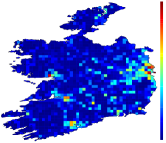
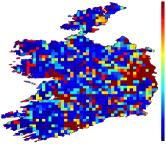
Figure 5: Reference scenario. Blue areas correspond to low demand, red ones to high demand. The left plot refers to the present time, i.e., $k=1$, the right plot to $k=K=60$ months.

We study the performance of our algorithms and the factors affecting it in a large-scale, real-world scenario. In this section we describe our reference topology and traffic demand, as well as the simulator we employ.

Topology We leverage two demand and deployment traces, provided by two Irish operators. They consist of two weeks of call-detail records (CDR) information for both voice and data traffic, collected over the whole Republic of Ireland. They include position, (approximate) coverage, and sectorization information for over 6,000 base stations, which constitute our set $\mathcal{B}$. For each base station $b$, the corresponding type $\mathcal{T}(b)$ (e.g., GSM, 3G, LTE) is also given.

Traffic demand We populate the set $\mathcal{C}$ of subscriber clusters by sampling Ireland’s territory according to the demographic data supplied by the Irish Central Statistics Office [13] in such a way that each of them accounts for (i) at most $500$ people and (ii) at most $5~{}km^{2}$. By doing this we place around 31,000 subscriber clusters in our topology. We experimented with different population and area limits, obtaining essentially the same results we present later. Traffic demand $\tau(c,o,1)$ at the present time slot $k=1$ is obtained from the traces and summarized in the left plot of Fig. 5. Future demand is projected according to the Cisco forecast [1]. Our time horizon is $|\mathcal{K}|=60$ time periods, with each period representing one month. The total demand for $k=K=60$, represented on the right-hand side of Fig. 5, is six times the initial one.

Simulation and updates The sheer scale of our reference topology rules out network simulators such as ns-2 and OMNeT++; rather, we resort to a custom simulator written in Python. The SINR and throughput between any (base station, subscriber cluster) pair are computed through the OFCOM-vetted methodology in [14], under the assumption of a reuse factor of $1$. The fraction $\phi$ of clusters that must enjoy the target competition level is set to $0.7$, unless otherwise specified.

\psfrag{nil}{$t_{\emptyset}$}\includegraphics[width=195.12767pt]{states}

Figure 6: The base station types in $\mathcal{T}$ and the possible changes. 3G base stations can be decommissioned (orange arrow), i.e., have their type set to $t_{\emptyset}$. New LTE base stations can be created (dark green arrow), possibly in the same location as existing base stations, or have their capacity enhanced through sectorization (light green arrows).

We assume that the set of base station types $\mathcal{T}$ contains the following elements:

• the decommissioned type $t_{\emptyset}$;

• a type for 3G base stations;

• three types for LTE base stations, with different sectorizations.

The changes we can apply to the network are summarized in Fig. 6: we can decommission a 3G base station, or create a new LTE base station (possibly in the same location of an existing one), or enhance the capacity of an existing LTE base station by increasing the sectorization thereof. In the following, we will collectively refer to the last two operations as updates. It is worth stressing that these limitations are not inherent to our model, which is able to account for any kind of network update and to interface with any simulator (see Fig. 3), but merely a way to simplify (and speed up) our performance evaluation.

6 Results

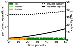
(a)

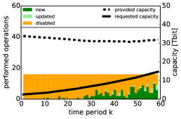
(b)

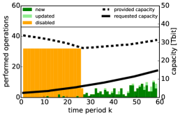
(c)

Figure 7: Changes applied to the network and requested and provided capacity for each time period $k$, when (a) $N=4~{}(=N_{\min})$, (b) $N=16$, (c) $N=32$.

We begin by looking at which network changes are performed at each time period $k$, and how they impact network capacity. In Fig. 7, solid and dotted lines correspond to requested traffic $\tau$ and provided capacity $\sigma$ respectively; bars represent the number of created, enhanced and decommissioned base stations. We are setting in the most favorable case: networks can be operated jointly and there is no competition constraint, i.e., $H_{\max}=1$.

Fig. 7(a) represents the case for $N=4$, the minimum possible value of $N$ in our scenario, as given by Eq. (7). It is easy to see that the value of $N$ directly maps to the maximum height of the bars. Very low values of $N$, as in Fig. 7(a), imply that most of the changes operators are able to perform are updates (i.e., create or enhance base stations), so as to meet the demand goal Eq. (3). As $N$ increases, as in Fig. 7(b), we are able to decommission more base stations, and to push forward in time all the updates. For even larger values of $N$, we see that there are some time periods where we perform fewer operations than we could, i.e., $\sum_{b\in\mathcal{B},t\in\mathcal{T}}x(b,k,t)<N$, as it happens for $k>25$ in Fig. 7(c). This is because we scheduled to decommission all possible base stations at earlier times, as mandated by Line 7 in Alg. 3, and schedule all needed updates later in time, as in Line 11 of Alg. 1.

Looking at provided and requested capacity, we can notice that the provided capacity is always substantially higher than the demand. This is because we have to preserve the coverage in the entire topology, i.e., all subscriber clusters $c\in\mathcal{C}$. In sparsely populated areas, this inevitably translates into underutilized base stations that operators have no way to decommission. It is also interesting to see how $N$ influences the evolution of provided capacity: low values of $N$ imply that the capacity slowly increases as updates are performed (Fig. 7(a)). Higher values of $N$, as in Fig. 7(b), mean that we can observe the behavior we were expecting in Fig. 1, with network capacity first slowly decreasing due to decommissioning base stations and then leveling up due to the concurrent scheduling of updates and decommissions. As we can see from Fig. 7(c), further increasing $N$ implies that network capacity decreases more swiftly (as operators can be quicker at decommissioning base stations) and increases more quickly afterwards, as most updates take place. Both effects are consistent with our intuition and expectations (Fig. 1): being able to perform more changes to the network means being more effective in tracking the traffic demand.

In Fig. 8 we look at the benefits of sharing, i.e., what savings operators can obtain by operating and updating their networks in a shared fashion. Fig. 8(a) is fairly clear – the benefits of sharing are very significant. The main effect of allowing sharing is that operators can save substantially more on operational costs, i.e., decommissioning more base stations. Sharing also reduces the unused capacity, which however remains quite significant, due to coverage requirements, as we already observed from Fig. 7.

The maps in Fig. 8(b) and Fig. 8(c) show where base stations are updated and decommissioned. Focusing on Fig. 8(b), which refers to the case where no sharing is allowed, we can observe that most updates are concentrated in densely populated areas (e.g., Dublin in the East), but some take place also in rural areas. On the other hand, virtually all decommissioned base stations are located in rural and suburban areas. Allowing sharing and moving to Fig. 8(c), we see a very different picture. In rural areas operators have to update much fewer base stations and can decommission many more; furthermore, many base stations can be decommissioned also in urban areas, e.g., in Dublin.

Put together, these results confirm the intuitive notion that network sharing directly translates into better network efficiency. Backed by our real-world demand and deployment traces, we can add that said efficiency is mostly attained by decommissioning underutilized base stations and, to a lesser extent, by pooling updated ones. Location-wise, we can say that network updates have the overall effect of migrating capacity from rural areas to urban ones, and sharing makes such an effect more pronounced, taking advantage of the redundancies of deployments, in particular in the rural areas.

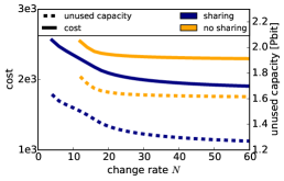
(a)

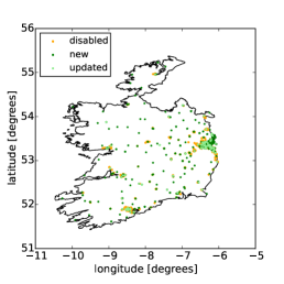
(b)

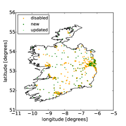
(c)

Figure 8: Unused capacity and cost savings (as defined in Eq. (5)) as a function of $N$ with and without sharing (a); location of updated and decommissioned base stations without (b) and with (c) sharing.

Competition regulation brings its own requirements on network planning, in particular mandating a certain level of extra capacity which could be used by a potential new virtual provider. In Fig. 9, we investigate the effects of competition regulation on the evolution of the network infrastructure. Recall that $H_{\max}=1$ means that there is no regulation in place, while $H_{\max}=0.5$ corresponds to the most stringent regulation, imposing as much as 50% idle capacity.

Fig. 9(a) confirms that the tighter the competition regulation, the lower the savings operators are able to achieve. As expected, moving from the most loose to the tightest level of regulation also increases the unused capacity – i.e., from the regulator’s viewpoint, the capacity available to new operators. In fact, imposing a minimum competition level has a double effect: first, it forces the operators to perform some updates that otherwise would have not been necessary to meet the capacity goal in Eq. (3); second, it restrains the operators from decommissioning some underutilized base stations. Intuitively, since most of the decommissioning would take place in the rural areas and most of the updates in cities (Fig. 8(c)), the regulation has the effect that users from both sparsely and densely populated areas are able to choose between more (actual or potential) operators.

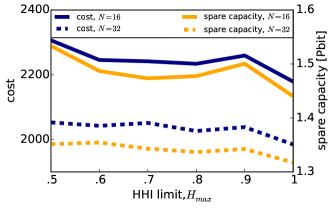
(a)

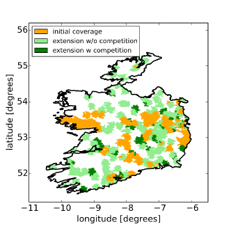
(b)

Figure 9: Unused capacity and cost (as defined in Eq. (5)) as a function of HHI index and for different values of $N$ (a); LTE coverage at $k=0$ (orange), $k=K=60$ when $H_{\max}=1$ (light green), and at $k=K=60$ when $H_{\max}=0.5$ (dark green).

Fig. 9(b) gives us further insights on the effect of competition regulation on LTE coverage. Specifically, it shows which areas are covered by LTE in the original deployment (i.e., $k=0$), which additional areas are covered at $k=K=60$ if $H_{\max}=1$, i.e., no competition regulation is in place, and which additional areas are covered at $k=K=60$ if $H_{\max}=0.5$. By forcing the installation of more base stations throughout different areas of the country, the regulators are also stimulating the deployment of newest technology in areas that otherwise the operators would not find attractive.

As newer technologies are deployed throughout the country, while the older ones tend to be dismissed, it is interesting to see if the traffic follows the same trend. In Fig. 10(b) we consider a moderate change rate ($N=16$) and different levels of competition, and present how much traffic will be served through 3G and 4G. A first observation we can make concerns the role of 3G – it will always serve a substantial share of the demand. Remarkably, this is exactly what the Cisco VNI foresees [1].

Increasing the level of competition, i.e., going from Fig. 10(a) to Fig. 10(b) has the effect of increasing the share of 4G traffic. This is essentially due to the fact that more 4G infrastructure is deployed, and users tend to prefer 4G over 3G when they can choose.

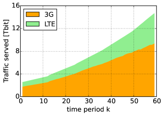
(a)

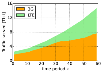
(b)

Figure 10: Traffic served per technology for each time period $k$, when $H_{\max}=1$ (a), and $H_{\max}=0.5$ (b).

As a result, our model is able to capture the tradeoff between savings and the promotion of innovations which is one of the main goals of regulators in the telecommunication industry.

7 Related work

Our work studies the effects of infrastructure sharing and competition regulation on cellular network planning.

The classic network planning problem usually considers a single operator that aims at minimizing operational costs for a specific technology (e.g. 3G, LTE) while maintaining acceptable users satisfaction both in terms of coverage and capacity. The research following this line is vast and includes various aspects. For example, in [15, 16, 17, 18, 19, 20, 21] the authors study the optimization of base station location in an area of interest. Some of these works [15, 16, 17, 18] deal with 3G systems and they are based on meta-heuristics aiming at minimizing the number of base stations to be deployed. Other more recent works [19, 20, 21] have focused on the same objective using similar approaches but on LTE networks.The work in [20] in particular uses a model based on stochastic geometry, and the coverage probability as the metric to optimize. The problem addressed in our paper is fundamentally different from the ones addressed by the aforementioned works since it includes sharing of already existing infrastructure by more than one operator and considers the competition regulation impact, modeled similarly as imposed by the Irish regulator recently [5], on network planning.

Resource sharing in inter-operator cellular networks, in fact, is another important aspect of our work and it has been studied in [22, 23, 2, 24]. In [22] the authors analyze feasible sharing options in the near-term in LTE using co-located and non co-located base stations. Authors in [23] assess the benefit of sharing both infrastructure and spectrum, using real base station deployment data. In [2] the authors have studied sharing opportunities between two operators, by looking at spatial variation in demand peaks. All the results obtained in these works suggest that resource sharing, whether spectrum or infrastructure, increases the network capacity and the ability to satisfy users’ requirements. However none of them addresses the problem of how to efficiently plan a shared network composed by resources already deployed by existing operators. In our previous work [24] we investigate the coverage efficiency obtained by combining existing cellular networks considering the coverage redundancy in real deployments in Poland but, unlike this paper, our earlier work does not address capacity requirements nor regulatory constraints.

Demographic data are an important source of information for operators to make planning decisions. Combining such data with the traffic demand information at their base stations, operators can have a clearer picture of the needed planning interventions. Researchers rarely use real topologies and demographic data; they typically rely on simplified synthetic topologies often featuring regular, lattice-like deployments that do not reflect the complexity and heterogeneity of cellular networks. Among the studies that uses real data that are related to our work are [24] and [23], that however do not use traffic demand data.

Other works use traffic demand, either concentrating on profiling the users  [25, 26, 27], or focusing more on the network behaviour  [8, 28, 27, 29] but none of them investigates long term planning decisions. The work in [8] is of interest to us because it has an objective orthogonal to ours; it is focused on energy savings and green networking and envisions dynamically switching off base stations at off-peak times in different parts of the topology. Our work instead aims at reconfiguring the whole network, operating long-term (possibly, permanent) changes in its infrastructure. It is important to stress that the two approaches can, and indeed should, coexist: once we reconfigure the infrastructure through our network sharing scheme, we can manage it in an energy-efficient fashion.

Works such as [30] focus on economic aspects of resource sharing from a network virtualization perspective. It describes the incentives operators have to pool their resources together. From an implementation perspective, the analysis of cooperative sharing arrangements presented in [31] highlights the diversity of approaches currently being used in existing networks, their successes and failures. It points to a process of learning within industry as to which sharing modes allow for both competition and cooperative sharing to thrive. A study of Pakistan’s experience of network sharing indicates the varying economic gains made in a still-developing market by adopting different sharing strategies [11].

However, while these papers address some of the economic effects of sharing, none of these has dealt with regulatory concerns regarding the ensuing market concentration which occurs through network sharing in mature mobile markets. Our study is unique because it combines all the aforementioned aspects (real data analysis, spatial distribution of traffic, network sharing, and network planning), and it considers the impact of the limitations imposed by the regulators on the savings when managing two networks in a shared fashion in a mature market.

8 Conclusion

We studied the modernization phase cellular networks will go through in the near future: mobile operators will decommission some underutilized base stations in order to save on costs, and deploy new-generation base stations in order to cope with the increasing demand. Operators can join forces and perform said changes in a shared way, so as to improve the efficiency of their networks. Operators’ ability to share infrastructure may be constrained by competition regulation, and the speed with which operators can make changes to their own networks may also be limited by practical considerations. We incorporate both factors in out study of cellular network planning.

Our first contribution is a general framework that describes network modernization scenarios, accounting for real topologies and demand information, and including multiple base station technologies. This model was presented in Sec. 2. Given our model and a limited budget of changes to perform at each time period, we presented in Sec. 3 a family of algorithms able to schedule the changes in a cost effective manner, while satisfying the demand and complying with regulatory constraints. These algorithms work unmodified whether operators perform their updates individually or in a shared fashion and, as shown in Sec. 4, return quasi-optimal solutions with a very small computational complexity, dominated by their sorting stage.

We apply our algorithms in a large-scale scenario, built from real-world demand and deployment traces as described in Sec. 5. As summarized in Sec. 6, we found that network modernization essentially means moving capacity from rural, sparsely populated areas (where many base stations can be decommissioned) to urban ones (where most of the new-generation base stations are located). Allowing sharing, i.e., permitting operators to jointly update and manage their networks, greatly enhances their effectiveness. Such benefits are reduced if tight competition rules are in place, but never entirely jeopardized. Indeed, tight competition regulations have the secondary effect of stimulating operators to extend the capacity and coverage of their new-generation networks, which can therefore serve a larger fraction of their demand.

Appendix: Proofs

Property 1.

Both goal 1 and goal 2 can be reached through network capacity-preserving changes alone, i.e., changes that comply with Eq. (6).

Proof:

Goal 1 means to satisfy Eq. (3) for all subscriber clusters $c\in\mathcal{C}$ and time periods $k\in\mathcal{K}$. If this is not the case, then the solution is scheduling updates that increase capacity. Decreasing the capacity for some subscriber clusters, i.e., breaking Eq. (6), is never necessary. A similar but slightly different reasoning holds for goal 2. Increasing the $\sigma$-values, as we can see from Eq. (2), decreases the HHI. ∎

Property 2.

If the initial configuration satisfies goal 1, then pursuing goal 2 by scheduling further capacity-preserving changes does not compromise goal 1.

Proof:

Once again, let us look at Eq. (3): if it holds, then all $\sigma$-values are no lower than the corresponding $\tau$-ones, therefore, there is no way that further increasing the $\sigma$-values can change this. ∎

Property 3.

The worst-case, combined time complexity of all our algorithms is $O(|\mathcal{B}|log|\mathcal{B}|)$.

Proof:

At each iteration of each of our algorithms, we make exactly one decision, i.e., set one $x$-value to $1$. Even if each base station is updated once to each possible type, the total number of decisions is still bounded by $|\mathcal{T}||\mathcal{B}|$, under the reasonable assumption that $|\mathcal{B}|\gg|\mathcal{T}|$, dominated by the sorting in Line 5 in Alg. 3, which has complexity $O(|\mathcal{B}|\log|\mathcal{B}|)$. ∎

Property 4.

If a set of changes satisfies Eq. (7), then Alg. 1 is able to schedule it.

Proof:

Scheduling a set of changes means enacting each of them at time $\hat{k}\leq k^{\star}$ no later than its deadline. In other words, every time we reach Line 11 in Alg. 1, the set $\{h\in\mathcal{K}:\sum_{b\in\mathcal{B},t\in\mathcal{T}}x(b,h,t)<N\wedge h\leq k^{\star}\}$ must be non-empty. In Line 7, we always select to schedule the base station with the lowest value of $k^{\star}$. This means that if at the current iteration we are scheduling a change due at time period $k^{\star}$, then all the changes we scheduled so far were due at $k^{\star}$ or earlier.

Since Eq. (7) holds, the number of such changes it at most $Nk^{\star}-1$; therefore, there must be a $\hat{k}$ between $1$ and $k^{\star}$ for which fewer than $N$ changes have been scheduled. Hence, the set is non-empty. ∎

Property 5.

The schedule returned by Alg. 1 minimizes the quantity in Eq. (8).

Proof:

We prove the property by induction.

Initialization. At the first iteration of Alg. 1, all $x$-values are set to $0$, thus in Line 11 we have $\hat{k}=k^{\star}$. The value of the quantity in Eq. (8) is zero, hence the schedule is optimal.

Induction step. Suppose all other changes have been scheduled optimally, i.e., they cannot be moved forward in time. Alg. 1 will try (Line 11) to schedule the current change for period $k^{\star}$, then $k^{\star}-1$, and so on, stopping at the latest feasible time. It follows that the resulting schedule still has the lowest possible value of Eq. (8). ∎

References

- [1] Cisco, “Cisco Visual Networking Index: Global Mobile Data Traffic Forecast Update, 2013-2018.” [Online]. Available: http://www.cisco.com/c/en/us/solutions/collateral/service-provider/visual-networking-index-vni/white_paper_c11-520862.pdf
- [2] P. Di Francesco, F. Malandrino, and L. A. DaSilva, “Mobile Network Sharing Between Operators: A Demand Trace-Driven Study,” in ACM SIGCOMM Capacity Sharing Workshop (CSWS), 2014.
- [3] B. Leng, P. Mansourifard, and B. Krishnamachari, “Microeconomic Analysis of Base-station Sharing in Green Cellular Networks,” in IEEE International Conference on Computer Communications (INFOCOM), 2014.
- [4] L. Doyle, J. Kibiłda, T. Forde, and L. A. DaSilva, “Spectrum without Bounds, Networks without Borders,” Proceedings of the IEEE, vol. 102, no. 3, pp. 351–365, 2014.
- [5] RTE News, “Vodafone criticises Three-O2 merger terms,” 2014. [Online]. Available: http://www.rte.ie/news/business/2014/0529/620446-vodafone-three-criticism/
- [6] M. A. Marsan and M. Meo, “Energy efficient management of two cellular access networks,” SIGMETRICS Perform. Eval. Rev., vol. 37, no. 4, pp. 69–73, Mar. 2010. [Online]. Available: http://doi.acm.org/10.1145/1773394.1773406
- [7] E. Oh, B. Krishnamachari, X. Liu, and Z. Niu, “Toward dynamic energy-efficient operation of cellular network infrastructure,” Communications Magazine, IEEE, vol. 49, no. 6, pp. 56–61, June 2011.
- [8] C. Peng, S.-B. Lee, S. Lu, H. Luo, and H. Li, “Traffic-driven power saving in operational 3G cellular networks,” in ACM International Conference on Mobile Computing and Networking (MobiCom), 2011.
- [9] U.S. Department of Justice and the Federal Trade Commission, “Horizontal merger guidelines,” Tech. Rep., August 2010.
- [10] European Commission, “EU Competition Law Rules Applicable to Merger Control Situation as at 1 April 2010,” Tech. Rep., 2010.
- [11] M. Choudhary, H. Babar, H. Shakeel, and A. Abbas, “Economics of network sharing - a case study of mobile telecom sector in pakistan,” in Collaborative Computing: Networking, Applications and Worksharing, 2009. CollaborateCom 2009. 5th International Conference on, Nov 2009, pp. 1–6.
- [12] N. Alon, D. Moshkovitz, and S. Safra, “Algorithmic construction of sets for k-restrictions,” ACM Trans. Algorithms, vol. 2, no. 2, pp. 153–177, Apr. 2006. [Online]. Available: http://doi.acm.org/10.1145/1150334.1150336
- [13] [Online]. Available: http://www.cso.ie/en/census/census2011boundaryfiles/
- [14] “LTE Technical Modelling Revised Methodology,” OFCOM White Paper, 2012. [Online]. Available: http://stakeholders.ofcom.org.uk/binaries/consultations/award-800mhz/annexes/annex14.pdf
- [15] E. Amaldi, A. Capone, and F. Malucelli, “Planning UMTS Base Station Location: Optimization Models with Power Control and Algorithms,” IEEE Transactions on Wireless Communications, vol. 2, no. 5, 2003.
- [16] C. Lee and H. Kang, “Cell Planning with Capacity Expansion in Mobile Communications: a TABU Search Approach,” IEEE Transactions on Vehicular Technology, vol. 49, no. 5, 2000.
- [17] A. Abdel-Khalek, L. Al-Janj, and Z. Dawy, “Optimization Models and Algorithms for Joint Uplink/Downlink UMTS Radio Network Planning with SIR-Based Power Control,” IEEE Transactions on Vehicular Technology, vol. 60, no. 4, 2011.
- [18] L. Shangyun and M. St-Hilaire, “A Genetic Algorithm for the Global Planning Problem of UMTS Netowrks,” in IEEE Global Communications Conference (GLOBECOM), 2010.
- [19] F. Gordejuela-Sanchez and J. Zhang, “LTE Access Network Planning adn Optimization: A Service Oriented and Technology-Specific Prospective,” in IEEE Global Communications Conference (GLOBECOM), 2009.
- [20] A. Guo and M. Haenggi, “Spatial Stochastic Models and Metrics for the Structure of Base Stations in Cellular Networks,” IEEE Transactions on Wireless Communications, vol. 12, no. 11, 2013.
- [21] H. Ghazzai, E. Yaacoub, M. S. Alouini, Z. Dawy, and A. Abu-Dayya, “Optimized LTE Cell Planning with Varying Spatial and Temporal User Densities,” IEEE Transactions on Vehicular Technology, vol. PP, no. 99, 2015.
- [22] J. S. Panchal, R. D. Yates, and M. M. Buddhikot, “Mobile Network Resource Sharing Options: Performance Comparisons,” IEEE Transactions on Wireless Communications, vol. 12, no. 9, pp. 4470–4482, 2013.
- [23] S. Hua, P. Liu, and S. S. Panwar, “The Urge to Merge: When Cellular Service Providers Pool Capacity,” in IEEE International Conference on Communications (ICC), 2012.
- [24] J. Kibiłda and L. A. DaSilva, “Efficient Coverage through Inter-operator Infrastructure Sharing in Mobile Networks,” in Wireless Days, 2013.
- [25] M. Z. Shafiq, L. Ji, A. Liu, J. J. Pang, and J. Wang, “Characterizing Geospatial Dynamics of Application Usage in a 3G Cellular Data Network,” in IEEE International Conference on Computer Communications (INFOCOM), 2012.
- [26] R. Keralapura, A. Nucci, Z. L. Zhang, and L. Gao, “Profiling users in a 3G network using hourglass co-clustering,” in ACM International Conference on Mobile Computing and Networking (MobiCom), 2011.
- [27] U. Paul, A. Subramanian, M. Buddhikot, and S. Das, “Understanding Traffic Dynamics in Cellular Data Networks,” in IEEE International Conference on Computer Communications (INFOCOM), 2011.
- [28] D. Willkomm, S. Machiraju, J. Bolot, and A. Wolisz, “Primary Users in Cellular Networks: A Large-Scale Measurement Study,” in IEEE Symposium on New Frontiers in Dynamic Spectrum Access Networks (DySPAN), 2008.
- [29] U. Paul, A. Subramanian, M. Buddhikot, and S. Das, “Understanding Spatial Relationships in Resource Usage in Cellular Data Networks,” in IEEE International Workshop on Network Science for Communication Networks (NetSciCom), 2012.
- [30] C. Courcoubetis and R. Weber, “Economic Issue in Shared Infrastructures,” IEEE/ACM Transactions on Networking, vol. 20, no. 2, pp. 594–608, 2012.
- [31] J. Markendahl and B. G. Molleryd, “On co-opetition between mobile network operators: Why and how competitors cooperate,” International Telecommunications Society (ITS), 19th ITS Biennial Conference, Bangkok 2012: Moving Forward with Future Technologies - Opening a Platform for All 72491, 2012.