The Evolution and Impacts of Magnetorotational Instability in Magnetized Core-Collapse Supernovae

Abstract

We carried out 2D-axisymmetric MHD simulations of core-collapse supernovae for rapidly-rotating magnetized progenitors. By changing both the strength of the magnetic field and the spatial resolution, the evolution of the magnetorotational instability (MRI) and its impacts upon the dynamics are investigated. We found that the MRI greatly amplifies the seed magnetic fields in the regime where not the Alfvén mode but the buoyant mode plays a primary role in the exponential growth phase. The MRI indeed has a powerful impact on the supernova dynamics. It makes the shock expansion faster and the explosion more energetic, with some models being accompanied by the collimated-jet formations. These effects, however, are not made by the magnetic pressure except for the collimated-jet formations. The angular momentum transfer induced by the MRI causes the expansion of the heating region, by which the accreting matter gain an additional time to be heated by neutrinos. The MRI also drifts low-$Y_{p}$ matter from the deep inside of the core to the heating region, which makes the net neutrino heating rate larger by the reduction of the cooling due to the electron capture. These two effects enhance the efficiency of the neutrino heating, which is found to be the key to boost the explosion. Indeed we found that our models explode far more weakly when the net neutrino heating is switched off. The contribution of the neutrino heating to the explosion energy could reach 60% even in the case of strongest magnetic field in the current simulations.

1. Introduction

Magnetic field and rotation are ubiquitous in stars. MiMeS survey has observed over 550 Galactic O- and B-type stars, and detected the surface magnetic fields of $\gtrsim 100$ G for $\sim 10$ % of them (see Wade & the MiMeS Collaboration (2014) for review). Estimating the upper limit of the currently-undetected magnetic field to be $\sim 100$ G, Wade & the MiMeS Collaboration (2014) argued that the distribution of the magnetic fields for massive stars may be bimodal: a small population of strong magnetic fields ($\gtrsim 1$ kG) and a large majority of weak magnetic fields ($\lesssim 100$ G). A magnetic field of 1 kG corresponds to the magnetic flux of $\sim 10^{27}$ G cm² for a 17 $M_{\odot}$ star with the radius of $\sim 8R_{\odot}$ (McNally, 1965), which is comparable to that of magnetars.

Ramírez-Agudelo et al. (2013) measured the surface rotational velocities of 216 O-type stars, and found that 25 % of the sample have $v\sin i>200$ km s^-1 while the rest of them are slow rotators. According to stellar evolution calculations by Woosley & Heger (2006), if a star is rotating fast enough initially, the rotational mixing prevents a very efficient angular momentum transport between the helium core and the hydrogen envelope, and the central iron core maintains a large amount of angular momentum at pre-collapse stage. They inferred the rotation period of a neutron star to be 2.3–9.7 ms for such evolutions of a 16 $M_{\odot}$ star with solar metallicity. Then, the high-rotational-velocity population found by Ramírez-Agudelo et al. (2013) might produce proto-neutron stars rotating with a period similar to those of millisecond pulsars (MSPs).

The influences of magnetic field and rotation on core-collapse supernovae have been studied as a possible agent to drive explosion other than neutrino heating, while the latter fails to produce energetic explosions (e.g., Suwa et al., 2010; Müller et al., 2012; Bruenn et al., 2013). MHD core-collapse simulations done so far have placed the main focus on rather extreme cases, viz., $B_{\textrm{pre}}\sim 10^{12}$–$10^{13}$ G and $\Omega_{\textrm{pre}}\sim 1$ rad s^-1 at pre-collapse, which correspond to the magnetar-class magnetic field and MSP-class rotation (e.g., Yamada & Sawai, 2004; Obergaulinger et al., 2006; Burrows et al., 2007; Shibata et al., 2006; Scheidegger et al., 2008, 2010; Sawai et al., 2013a; Mösta et al., 2014). In those simulations, the magnetic field wound by differential rotation grows to dynamically important strengths and later drives a strong outflow along the rotation axis, reproducing the typical supernova-explosion energy of $E_{\textrm{exp}}\sim 10^{51}$ erg.

Since the magnetic field and rotation in massive stars are likely to have wide range of values as mentioned above, it may be also important to study more ”ordinary” cases. In these cases amplification mechanisms that are more efficient than the simple winding are imperative to produce the field strength of $\sim 10^{15}$ G outside the proto-neutron star, which may be necessary to impact on the supernova dynamics. For non-rotating case Endeve et al. (2010, 2012) numerically studied the standing accretion shock instability, while Obergaulinger et al. (2014) investigated the convection. In both cases, the amplification is rather modest, and the impacts on dynamics are found to be minor.

If the iron core is initially rotating rapidly, another candidate of an efficient field amplification mechanism in core-collapse supernovae is the magnetorotational instability (MRI), which basically occurs in differentially rotating systems (Balbus & Hawley, 1991; Akiyama et al., 2003). Simulations of the MRI for weak seed magnetic fields are computationally demanding, since the wavelength of the fastest growing mode is quite small compared with the size of the iron core, $\sim 1000$ km:

$$\lambda_{\textrm{FGM}} \sim \frac{2\pi v_{\textrm{A}}}{\Omega}$$

$$\sim 200\textrm{m}\left(\frac{\rho}{10^{12}\textrm{g cm}^{-1}}\right)^{-\frac{1}{2}}\left(\frac{B}{10^{13}\textrm{G}}\right)\left(\frac{\Omega}{10^{3}\textrm{rad s}^{-1}}\right)^{-1},$$

where $v_{\textrm{A}}$ is Alfvén velocity. In fact, most of previous core-collapse simulations assuming sub-magnetar-class magnetic fields have insufficient spatial resolutions to capture the MRI (Moiseenko et al., 2006; Burrows et al., 2007; Takiwaki et al., 2009). In order to resolve the fastest growing mode, local simulation boxes are utilized in some 2D/3D computations (Obergaulinger et al., 2009; Masada et al., 2012; Guilet Müller, 2015; Rembiasz et al., 2015). The problems in the local simulations, however, are the difficulties in taking into account the effects from and feedbacks to dynamically changing structures.

Sawai et al. (2013b) conducted the first global core-collapse simulations for sub-magnetar-class magnetic fields with a sufficient spacial resolution to capture the MRI albeit in 2D axisymmetry, and found that the magnetic field is amplified by the MRI to dynamically important strengths. In order to study its impacts on the global dynamical, Sawai & Yamada (2014) carried out similar but longer-term simulations up to several hundred milliseconds after bounce, employing the simple light bulb approximation for neutrino transfer. They found that the MRI indirectly enhances the neutrino heating, and thus boost the explosion. Performing 3D simulations for a thin layer on the equator, Masada et al. (2015) argued another possible effect of the MRI, i.e., the enhancement of neutrino luminosity by MRI-driven turbulence around the proto-neutron star surface.

This paper is a sequel to Sawai et al. (2013b) and Sawai & Yamada (2014). We conducted 2D-axisymmetric high-resolution simulations of core-collapse for rapidly-rotating magnetized progenitors, changing the initial magnetic field strength and the spatial resolution. The initial magnetic field strength assumed here, $B_{\textrm{pre}}\sim 10^{11}$ G, are one or two orders of magnitude smaller than the extreme values adopted in some previous simulations mentioned above.

The rest of the paper is organized as follows. In Section 2, we describe the numerical method and models. The results are presented in Section 3, and the discussion and conclusion are given in Section 4.

2. Numerical Methods

We adopt a $15M_{\odot}$ star (Woosley & Weaver, 1995) for the progenitor of core-collapse simulations, adding magnetic fields and rotations by hand. The following ideal MHD equations and the equation of electron number density are numerically solved by a time-explicit Eulerian MHD code, Yamazakura (Sawai et al., 2013a):

$$\frac{\partial\rho}{\partial t}+\nabla\cdot(\rho\mbox{\boldmath$v$})=0,$$ (2)

$$\frac{\partial}{\partial t}(\rho\mbox{\boldmath$v$})+\nabla\cdot\left(\rho\mbox{\boldmath$v$}\mbox{\boldmath$v$}-\frac{\mbox{\boldmath$B$}\mbox{\boldmath$B$}}{4\pi}\right)$$

$$\hskip 12.0pt=-\nabla\left(p+\frac{B^{2}}{8\pi}\right)-\rho\nabla\Phi,$$ (3)

$$\frac{\partial}{\partial t}\left(e+\frac{\rho v^{2}}{2}+\frac{B^{2}}{8\pi}\right)$$

$$\hskip 12.0pt+\nabla\cdot\left[\left(e+p+\frac{\rho v^{2}}{2}+\frac{B^{2}}{4\pi}\right)\mbox{\boldmath$v$}-\frac{(\mbox{\boldmath$v$}\cdot\mbox{\boldmath$B$})\mbox{\boldmath$B$}}{4\pi}\right]$$

$$\hskip 48.0pt=-\rho(\nabla\Phi)\cdot\mbox{\boldmath$v$}+Q_{E}^{\textrm{abs}}+Q_{E}^{\textrm{em}},$$ (4)

$$\frac{\partial\mbox{\boldmath$B$}}{\partial t}=\nabla\times\left(\mbox{\boldmath$v$}\times\mbox{\boldmath$B$}\right),$$ (5)

$$\frac{\partial n_{e}}{\partial t}+\nabla\cdot(n_{e}\mbox{\boldmath$v$})=Q_{N}^{\textrm{abs}}+Q_{N}^{\textrm{em}},$$ (6)

where $Q_{E}^{\textrm{abs}}$ and $Q_{E}^{\textrm{em}}$ are the changes of energy density due to neutrino/anti-neutrino absorptions and emissions, respectively, and $Q_{N}^{\textrm{abs}}$ and $Q_{N}^{\textrm{em}}$ are the similar notations for the changes of electron number density. The other symbols have their usual meanings. The electron fraction, $Y_{e}$, is given by the prescription suggested by Liebendörfer (2005) until bounce. After that, where Liebendörfer’s prescription is no longer valid, Equation (6) is solved to obtain $Y_{e}=n_{e}m_{u}/\rho$, where $m_{u}=1.66\times 10^{-24}$ g is the atomic mass unit. We assume Newtonian mono-pole gravity. A tabulated nuclear equation of state produced by Shen et al. (1998a, b) is utilized. Computations are done with polar coordinates in two dimensions, assuming axisymmetry and equatorial symmetry.

We take into account interactions of electron neutrinos $\nu_{e}$ and anti-neutrinos $\bar{\nu}_{e}$ with nucleons. Instead of dealing with detailed neutrino transport, the light bulb approximation is used as in Murphy et al. (2009); Nordhaus et al. (2010); Hanke et al. (2012). Taking the ultra-relativistic limit for electrons and positrons, assuming the Fermi-Dirac distribution with vanishing chemical potential for $\nu_{e}$ and $\bar{\nu}_{e}$, and neglecting the phase space blocking, we evaluate the source term related to $\nu_{e}$/$\bar{\nu}_{e}$ absorption ($\nu_{e}+n\to e^{-}+p,\bar{\nu}_{e}+p\to e^{+}+n$) in the energy equation (4) as

$$Q_{E}^{\textrm{abs}}=\frac{3\alpha^{2}+1}{4}\frac{\sigma_{0}\langle\epsilon_{\nu_{e}}^{2}\rangle}{(m_{e}c^{2})^{2}}\frac{\rho}{m_{u}}\frac{L_{\nu_{e}}}{4\pi r^{2}\langle\mu_{\nu}\rangle}\left(Y_{n}+Y_{p}\right)$$ (7)

(Janka, 2001), where $\alpha=1.26$ is the charged-current axial-vector coupling constant, $\sigma_{0}=1.76\times 10^{-44}$ cm² the characteristic cross section of weak interaction, $\langle\epsilon_{\nu_{e}}^{2}\rangle=20.8\left(kT_{\nu_{e}}\right)^{2}$ the mean square neutrino energy, $m_{e}c^{2}=0.511$ MeV the rest-mass energy of electron, $L_{\nu_{e}}$ the neutrino luminosity, $r$ the distance from the center, and $\langle\mu_{\nu}\rangle$ the so-called flux factor. Here, we assume the same luminosity and spectral temperature for $\nu_{e}$ and $\bar{\nu}_{e}$. In the present simulations, $L_{\nu_{e}}=1.0\times 10^{52}$ erg s^-1, $kT_{\nu_{e}}=4.0$ MeV, and $\langle\mu_{\nu}\rangle=1.0$ are chosen. Similarly, the source term related to $\nu_{e}$/$\bar{\nu}_{e}$ absorption in the equation of $n_{e}$ (6) is

$$Q_{N}^{\textrm{abs}}=\frac{3\alpha^{2}+1}{4}\frac{\sigma_{0}\langle\epsilon_{\nu_{e}}\rangle}{(m_{e}c^{2})^{2}}\frac{\rho}{m_{u}}\frac{L_{\nu_{e}}}{4\pi r^{2}\langle\mu_{\nu}\rangle}\left(Y_{n}-Y_{p}\right),$$ (8)

where $\langle\epsilon_{\nu_{e}}\rangle=4.11\left(kT_{\nu_{e}}\right)$ is the mean neutrino energy.

The source term related to the $\nu_{e}$/$\bar{\nu}_{e}$ emission ($e^{-}+p\to\nu_{e}+n$, $e^{+}+n\to\bar{\nu}_{e}+p$) in Equation (4) is given by

$$Q_{E}^{\textrm{em}} = -\left(3\alpha^{2}+1\right)\frac{\pi\sigma_{0}c\left(kT\right)^{6}}{(hc)^{3}(m_{e}c^{2})^{2}}\frac{\rho}{m_{u}}$$ (9)

$$\times\left[Y_{n}\mathcal{F}_{5}(-\eta_{e})+Y_{p}\mathcal{F}_{5}(\eta_{e})\right]$$

(Janka, 2001), where $\eta_{e}$ is the electron chemical potential normalized by the temperature, and

$$\mathcal{F}_{l}(\eta)\equiv\int^{\infty}_{0}\frac{x^{l}}{1+\exp(x-\eta)}dx.$$ (10)

Similarly, the emission source term in Equation (6) is

$$Q_{N}^{\textrm{em}} = \left(3\alpha^{2}+1\right)\frac{\pi\sigma_{0}c\left(kT\right)^{5}}{(hc)^{3}(m_{e}c^{2})^{2}}\frac{\rho}{m_{u}}$$ (11)

$$\times\left[Y_{n}\mathcal{F}_{4}(-\eta_{e})-Y_{p}\mathcal{F}_{4}(\eta_{e})\right].$$

The Fermi integrals (Equation (10)) are calculated as follows:

$$\mathcal{F}_{4}(\eta_{e}) = 24\mathcal{I}_{4}(\eta_{e}),$$ (12)

$$\mathcal{F}_{5}(\eta_{e}) = 120\mathcal{I}_{5}(\eta_{e}),$$ (13)

$$\mathcal{F}_{4}(-\eta_{e}) = \frac{1}{5}\eta_{e}^{5}+\frac{2}{3}\pi^{2}\eta_{e}^{3}+\frac{7}{15}\pi^{4}\eta_{e}+24\mathcal{I}_{4}(\eta_{e}),$$ (14)

$$\mathcal{F}_{5}(-\eta_{e}) = \frac{1}{6}\eta_{e}^{6}+\frac{5}{6}\pi^{2}\eta_{e}^{4}+\frac{7}{6}\pi^{4}\eta_{e}^{2}$$ (15)

$$+\frac{31}{126}\pi^{6}+120\mathcal{I}_{5}(\eta_{e}),$$

where

$$\mathcal{I}_{l}(\eta)\equiv\sum_{m=1}^{\infty}\left[\frac{(-1)^{m-1}}{m^{l+1}}e^{-m\eta}\right].$$ (16)

The source terms given by Equations (7), (8), (9), (11) are valid only in optically thin regions, and must decrease toward the optically thick regions. To mimic such reduction they are multiplied by $e^{-\tau_{\textrm{eff}}}$, following Murphy et al. (2009). Here, the effective optical depth is defined as

$$\tau_{\textrm{eff}}=\int^{\infty}_{r}\kappa_{\textrm{eff}}(r)dr,$$ (17)

where the effective opacity is given as

$$\kappa_{\textrm{eff}}=1.2\times 10^{-7}\left(\frac{\rho}{10^{10}\textrm{g cm}^{-3}}\right)\left(\frac{kT_{\nu_{e}}}{4\textrm{MeV}}\right)\left(Y_{n}+Y_{p}\right),$$

from the Equations (10), (11), and (14) of Janka (2001).

Before conducting high-resolution simulations to capture the MRI, we first follow the collapse of the 15 $M_{\odot}$ progenitors until several 100 ms after bounce by low-resolution simulations, whose numerical domain spans from the radius of 100 m to 4000 km. We refer to these simulations as background (BG) runs. In the BG runs, the core is covered with $N_{r}\times N_{\theta}=720\times 60$ numerical grids, where the spatial resolution is 0.4–23 km.

The pre-collapse cores are assumed to be rapidly rotating with the initial angular velocity profile of

$$\Omega(r)=\Omega_{0}\frac{r_{0}^{2}}{r_{0}^{2}+r^{2}},$$ (19)

where $r$ is the distance from the center of the core. The parameters are chosen as $r_{0}=1000$ km and $\Omega_{0}=2.73$ rad s^-1, corresponding to a millisecond proto-neutron star after collapse. The initial rotational energy divided by the gravitational binding energy is $2.5\times 10^{-3}$.

We assume that the pre-collapse magnetic fields have dipole-like configurations produced by electric currents of a 2D-Gaussian-like distribution centered at $(\varpi,z)=(\varpi_{0},0)$,

$$j_{\phi}(\varpi,z) = j_{0}e^{-\tilde{r}^{2}/2\sigma(\tilde{\theta})^{2}}\left(\frac{\varpi_{0}\varpi}{\varpi_{0}^{2}+\varpi^{2}}\right),$$ (20)

where $(\varpi,z)$ are cylindrical coordinates, $\tilde{r}\equiv\sqrt{(\varpi-\varpi_{0})^{2}+z^{2}}$, $\tilde{\theta}\equiv\arccos(z/\tilde{r})$, and

$$\sigma(\tilde{\theta})=\frac{\tilde{r}_{\textrm{dec}}}{\sqrt{1-e^{2}\cos{\tilde{\theta}}}}$$ (21)

(Sawai et al., 2013a). Changing $j_{0}$, we perform three BG runs with different strengths of magnetic fields, where the maximum strengths at pre-collapse, $B_{\textrm{pre}}$, are 5.0$\times 10^{10}$, 1.0$\times 10^{11}$, and $2\times 10^{11}$ G. Hereafter we refer to these BG runs as B5e10bg, B1e11bg, and B2e11bg, respectively. The rest of parameters are set as $\varpi_{0}=\tilde{r}_{\textrm{dec}}=1000$ km and $e=0.5$ in all the computations. The initial magnetic energy divided by the gravitational binding energy is quite small, $2.1\times 10^{-6}$, even for the strongest-field model, B2e11bg. We also computed models without magnetic field and rotation as well as a model having rotation alone for comparison.

In order to capture the growth of MRI we conduct high-resolution simulations with the numerical domain spanning $50<(r/$km$)<500$ (referred to as MRI runs). The initial conditions of MRI runs are given by mapping the data of the BG runs onto the above domain at 5 ms after bounce. In order to satisfy the divergence free constraint on the magnetic field, not the magnetic field itself but the vector potential is mapped as in Sawai et al. (2013a). The inner and outer radial boundary conditions for the MRI runs are given by the data of the basic runs, except that the inner boundary conditions of $B_{r}$ are determined to satisfy the divergence-free condition. The grid spacing is such that the radial and angular grid sizes are the same, viz. $\Delta r=r\Delta\theta$, at the innermost and outermost cells. For each BG run, four MRI runs with different grid resolutions are carried out. Our choice of the resolution at $r=50$ km, $\Delta_{50}$, (and the numbers of grids, $N_{r}\times N_{\theta}$), is 12.5 m ($9250\times 6400$), 25 m ($4650\times 3200$), 50 m ($2300\times 1600$), and 100 m ($1160\times 800$). We label the MRI runs by the initial field strength of the corresponding BG run followed by the spatial resolution. For example, the MRI run using the data of model B5e10bg and $\Delta_{50}=12.5$ m is referred to as model B5e10$\Delta$12.5. For a set of models involving the same initial magnetic field, we use a term “model series”, e.g., models series B5e10.

In dealing with the MHD equations in the polar coordinates, we should be cautious about numerical treatments of the coordinate singularities at the center of the core ($r=0$) and the pole ($\theta=0$). In the vicinity of the pole, the regularity conditions demand that the expansions of $v_{\theta}$, $v_{\phi}$, $B_{\theta}$, and $B_{\phi}$ with respect to $\theta$ should not contain $\theta$-independent terms, which is not necessarily satisfied in numerical simulations. In order to numerically meet the regularity conditions in the vicinity of the pole albeit approximately, we remove the region of $\theta<0.3^{\circ}$ from the numerical domain and impose boundary conditions based on the regularity conditions except for $B_{\theta}$, which is determined by the divergence-free constraint. To diffuse undesirable fluctuations that tend to violate the regularity, we further introduce an artificial resistivity only at the cells closest to the pole in the form of

$$\eta_{\textrm{a}}=\frac{\alpha a_{\textrm{max}}\Delta^{2}}{l_{B}},$$ (22)

where $\alpha$ is a dimensionless factor, $a_{\textrm{max}}$ the local maximum characteristic speed, $\Delta$ the grid width, and $l_{B}$ the scale height of the magnetic field. The factor $\alpha$ is automatically controlled between 0.1–$10^{3}$ during the simulations depending on how well the regularity condition is satisfied.

In order to maintain the regularity conditions approximately around the center in the BG runs, we remove the central part within the radius of 100 m from the numerical domain and take a similar remedy.

3. Results

3.1. The Growth of MRI

The stability condition of the axisymmetric MRI for general rotation laws $\Omega(\varpi,z)$ is given by

$$\mathcal{C} \equiv \left(\mathcal{G}_{z}\mathcal{B}_{z}\tan^{2}\theta_{k}-2\mathcal{G}_{z}\mathcal{B}_{\varpi}\tan\theta_{k}+\mathcal{G}_{\varpi}\mathcal{B}_{\varpi}+\mathcal{R}_{\varpi}\right)/\Omega^{2}$$ (23)

$$> 0,$$

where $\theta_{k}$ is the angle between the perturbation wavenumber $k$ and the $z$-axis,

$$\mathcal{G} \equiv \frac{\nabla P}{\rho},$$ (24)

$$\mathcal{B} \equiv -\frac{1}{\Gamma}\frac{\partial\ln P}{\partial s}\Big{|}_{\rho,Y_{e}}\nabla s-\frac{1}{\Gamma}\frac{\partial\ln P}{\partial Y_{e}}\Big{|}_{\rho,s}\nabla Y_{e},$$ (25)

$$\mathcal{R} \equiv \varpi\nabla\Omega^{2},$$ (26)

and $\Gamma\equiv\partial\ln P/\partial\ln\rho|_{s,Y_{e}}$ (Balbus, 1995; Obergaulinger et al., 2009).

The MRI involves two distinct modes, namely, Alfvén mode and buoyant mode, where the former appears for $\mathcal{C}<0$, and the latter only emerges for $\mathcal{C}+4<0$ (Urpin, 1996). Which mode dominates over the other for a fixed $\theta_{k}$ depends on the value of $\mathcal{C}$ (Obergaulinger et al., 2009). For $-8<\mathcal{C}<0$, the fastest growing mode is the Alfvén mode with the wavenumber of

$$\mbox{\boldmath$k$}_{\textrm{FGM}}\cdot\mbox{\boldmath$v$}_{\textrm{A}}=\cos\theta_{k}\Omega\frac{\sqrt{-\mathcal{C}(\mathcal{C}+8)}}{4},$$ (27)

and the growth rate of

$$\omega_{\textrm{FGM}}=\cos\theta_{k}\Omega\frac{\sqrt{-\mathcal{C}^{2}}}{4}.$$ (28)

For $\mathcal{C}\leq-8$, the fastest growth occurs with

$$\omega_{\textrm{FGM}}=\cos\theta_{k}\Omega\sqrt{\mathcal{C}+4},$$ (29)

for $\mbox{\boldmath$k$}_{\textrm{FGM}}\cdot\mbox{\boldmath$v$}_{\textrm{A}}=0$, i.e., it is the buoyant mode.

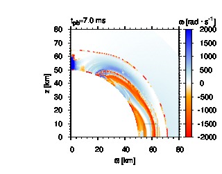
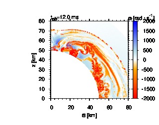
Figure 1.— Color maps of the dominant modes and growth rate for model B5e10$\Delta$12.5 at $t_{\textrm{pb}}=7$ (upper panel) and $t_{\textrm{pb}}=12$ (lower panel). The red and blue colors, respectively, represent the locations where buoyant mode and Alfvén mode are dominant. The growth rate is multiplied by -1 for buoyant-mode-dominant regions. The boxes in the upper panel correspond to the plot areas of Figure 3.

Since $\mathcal{C}$ depends on $\theta_{k}$, the dominant mode differs for different directions. In order to find the dominant mode for a fixed spatial point, we vary $\theta_{k}$ numerically in the range of $[-\pi/2:\pi/2]$. The result is shown in Figure 1 for model B5e10$\Delta$12.5 at the postbounce time of $t_{\textrm{pb}}=7$ and 12 ms, where the red and blue colors represent buoyant-mode- and Alfvén-mode-dominant regions, respectively, and the shades of the colors indicate the growth rate. It is evident that the dominant mode is different from location to location, and the regions dominated by the buoyant-mode have on average larger growth rates than those dominated by the Alfvén mode.

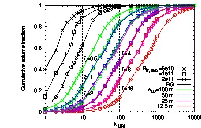
Figure 2.— Cumulative volume fractions having $N_{\textrm{MRI}}$ smaller than a given value for the all models.

The growth of the Alfvén-mode, although slower than the buoyant mode, still may have an important effect on the magnetic field amplification in the locations of its dominance. It is hence important to know how well we numerically resolve the fastest-growing Alfvén mode (FGAM), whose wave number is given by Equation (27). Figure 2 shows for all the models the cumulative fraction of the volume that has $N_{\textrm{MRI}}$ smaller than a given value. Here $N_{\textrm{MRI}}$ is defined at each point to be the ratio of the wavelength of FGAM to the grid size and is measure of how well FGAM is resolved numerically. We introduce to characterize the models, a factor $\xi\equiv\left(B_{\textrm{in,max}}/10^{11}\textrm{G}\right)(\Delta_{50}/100\textrm{m})^{-1}$, since only the initial strength of the magnetic field and spacial resolution are different among the current set of the models. In fact, similar distributions is obtained for the models having the same $\xi$ at early epochs when the magnetic field is almost passive (see Figure 2). According to Shibata et al. (2006), $N_{\textrm{MRI}}\gtrsim 10$ is required to capture the linear growth of the Alfvén mode. In our weakest-field model series B5e10, the volume fractions with $N_{\textrm{MRI}}\leq 10$ are 0.6, 0.27, 0.12, and 0.018 for models $\Delta$100 ($\xi=0.5$), $\Delta$50 ($\xi=1$), $\Delta$25 ($\xi=2$), and $\Delta$12.5 ($\xi=4$), respectively. We hence believe that our highest-resolution models should be able to capture the linear growth of the Alfvén mode well.

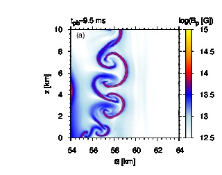
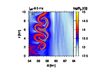
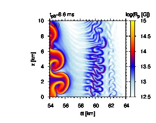
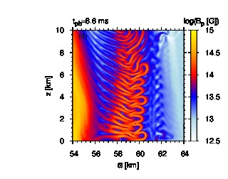
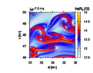
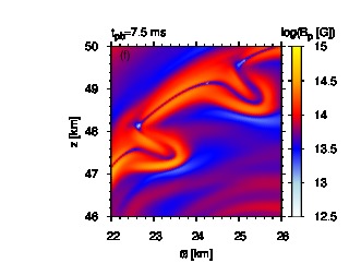
Figure 3.— Color maps for the strength of the poloidal magnetic field for models B5e10$\Delta$12.5 (left panels) and B2e11$\Delta$12.5 (right panels). The upper four panels zoom in a part of equatorial region (presented by the large box in the upper panel of Figure 1), while the lower two panels that of a middle-latitude region (the small box in the upper panel of Figure 1). Panels (c) and (d) are for models with initial perturbations.

In order to confirm that both the buoyant and Alfvén modes are growing indeed in the regions predicted in Figure 1, we examine the wavelengths of the growing modes in these regions. The upper panels of Figure 3 show the color maps of the poloidal magnetic field strength at $t_{\textrm{pb}}=9.5$ ms in a region around the equator, indicated by the large box in the upper panel of Figure 1, where two red belts of buoyant-mode dominance are observed. We found that the patterns of strong-magnetic-field filaments seen in the upper panels of Figure 3 have grown in the regions of buoyant-mode dominance: in the case of model B5e10$\Delta$12.5, this region corresponds to the right-side red belt observed in the large box indicated in the upper panel of Figure 5, which has been advected leftward during $t_{\textrm{pb}}=7.0$–$9.5$ ms. We compare models B5e10$\Delta$12.5 and B2e11$\Delta$12.5, which have different initial field strengths. As expected for the buoyant mode, the wavelengths of the growing modes, which are evaluated from the sizes of the patterns, are nearly identical between the two models. The wavelengths of the growing modes observed here may reflect the scale of the dominant perturbation, which may come from numerical noises. To see if this is true, we performed test simulations for the two models in which a perturbation of $u^{\prime}=u^{\prime}_{0}\sin(2\pi z/\lambda_{\textrm{prt}})$ is given at the beginning of the MRI runs, where the amplitude and the wavelength of the perturbation is set as 1% and 500 m, respectively. As a result, we found that the wavelengths of growing modes are shorter than those of the models without perturbation (see panels (c) and (d) of Figure 3), which indicates that the observed modes depend on the dominant scale of perturbations.

The lower panels of Figure 3 zoom in the area around $\theta=35^{\circ}$ in the vicinity of the inner boundary, where a pocket of buoyant-mode-dominant regions are surrounded by an Alfvén-mode-dominant region (see the small box in the upper panel of Figure 1). The wavelength of the growing mode there is shorter for the weaker initial field. In fact, the widths of protruding magnetic flux loops in the panel (e) of Figure 3 for model B5e10$\Delta$12.5 are about three times smaller than those in the panel (f) for model B2e11$\Delta$12.5. The ratio is close to four, the value expected for the Alfvén mode. With these facts, we believe that our simulations capture both the buoyant and Alfvén modes correctly.

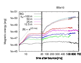
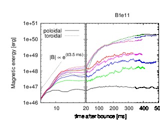
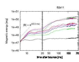
Figure 4.— Evolutions of the magnetic energies of the poloidal and toroidal components, integrated over the whole numerical domain, for model series B5e10 (upper panel), B1e11 (middle panel), and B2e11 (lower panel). Those for the MRI runs are plotted until the shock surface reaches the outer boundary in each model. Only those for model B2e11$\Delta$12.5 are plotted even after the shock passes the outer boundary in order to see a clear saturation of the magnetic energy of the poloidal component. The red crosses represent the moment when the shock surface reaches the outer boundary in model B2e11$\Delta$12.5.

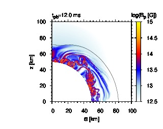
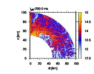
Figure 5.— Color maps for the strength of the poloidal magnetic fields for model B5e10$\Delta$12.5 at $t_{\textrm{pb}}=12$ ms (upper panel) and 200 ms (lower panel). The black line in the upper panel represents the shock surface.

Figure 4 plots the time evolutions of the magnetic energies, integrated over the whole numerical domain for all models. Those for the MRI runs are plotted until the shock surface reaches the outer boundary. Only in model B2e11$\Delta$12.5, the plots are continued for another 12 ms after the shock surface passes the outer boundary. Since the magnetic energies flowing out of the boundary during this 12 ms are found to be negligible, i.e., 0.81% and 0.24% of the total poloidal and toroidal magnetic energies at the end of the plot, respectively, we do not take them into account in the following discussion. The exponential growth of the energy of the poloidal component, $E_{B_{\textrm{p}}}$, is apparent during the first $\sim 10$ ms for all the MRI runs. In each model series, the growth timescale becomes shorter (or the growth rate is larger) for higher resolutions until it converges to $\approx$3–3.5 ms. These timescales well match the theoretical prediction for the buoyant-mode of $\sim$2000 rad s^-1, which is shown in the upper panel of Figure 1. This implies that the exponential growth is dominated by the buoyant mode. Indeed, the comparison between the lower panel of Figure 1 and the upper panel of Figure 5 indicates the coincidence of the locations, where the poloidal magnetic field is preferentially amplified, with those of buoyant-mode dominance at $t_{\textrm{pb}}=12$ ms, around the end of the exponential growth. From the numerical convergence we observed, it is suggested that the high spatial resolution is required even for the buoyant mode, in which all wavelengths grow at an equal rate.

After the exponential growth phase ceases, $E_{B_{\textrm{p}}}$ continues to increase gradually until it reaches saturation roughly around $t_{\textrm{pb}}=$210, 270, and 160 ms for model series B5e10, B1e11, and B2e11, respectively (see Figure 4). During this phase the region of strong magnetic field, say, $B>10^{14}$ G, spreads over a considerable volume inside the radius of $\sim 100$ km (see the lower panel of Figure 5 for B5e10$\Delta$12.5).

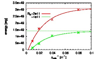
Figure 6.— The time-averaged saturation values of the magnetic energy of the poloidal component (crosses) and the fitted curves (solid lines) with respect to the resolution for model series B1e11 and B2e11. The dotted lines represent the saturation values, $a_{1}$.

As can be seen from each panel of Figure 4, the saturated values of $E_{B_{\textrm{p}}}$ do not converge, which may be because the turbulence is not yet fully captured due to numerical diffusivity (Sawai et al., 2013b). Nevertheless, since model series B1e11 and B2e11 show a trend of convergence, we may be able to estimate the converged values by fitting the time-averaged $E_{B_{\textrm{p}}}$ for the different resolution models with suitable functions. Taking the time averages over $t_{\textrm{pb}}=270$–330 ms and 165–185 ms for model series B1e11 and B2e11, respectively, we fitted the results with functions in the form of

$$\langle E_{B_{\textrm{p}},{\textrm{sat}}}\rangle=a_{1}-a_{2}\exp\left({-a_{3}/\Delta_{50}}\right),$$ (30)

where $a_{1}$, $a_{2}$, and $a_{3}$ are the parameters to be determined. The values obtained for $a_{1}$ are $1.4\times 10^{49}$ and $3.1\times 10^{49}$ erg for model series B1e11 and B2e11, respectively (see Figure 6). It is also found that the saturated values of $E_{B_{\textrm{p}}}$ for the highest-resolution models B1e11$\Delta$12.5 and B2e11$\Delta$12.5 are 91% and 96% of these values, respectively, i.e., they are close to convergence. Indeed, it is expected that if we were able to afford twice higher resolution, we could achieve convergence.

Our results also suggest that larger initial magnetic fields may result in larger saturated values. This is consistent with the results obtained by Hawley et al. (1995), who performed local box simulations of MRI in the context of accretion disks. Masada et al. (2015) also claimed that the saturation depends on the initial fields, however, no resolution study was done. As shown here, the resolution dependence should properly taken into account in discussing the saturation.

The magnetic energy of the toroidal component, $E_{B_{\textrm{t}}}$, also shows the exponential growth in each model (see Figure 4). Since the non-axisymmetric MRI for the toroidal components cannot be treated with the current simulations, this is not due to the MRI but due to the winding of the MRI-amplified poloidal component by differential rotation. This is understood from the fact that $E_{B_{\textrm{t}}}$ continuously increases even after the poloidal component is saturated and become one order of magnitude greater than $E_{B_{\textrm{p}}}$. At the end of the simulations, $E_{B_{\textrm{t}}}$ still continues to increase gradually in most of the models. Only for models B1e11$\Delta$25 and B1e11$\Delta$12.5, $E_{B_{\textrm{t}}}$ has nearly reached the saturated values. Incidentally, the numerical convergence is achieved in $E_{B_{\textrm{t}}}$ for model series B1e11 and B2e11.

3.2. Impacts on Global Dynamics

3.2.1 Background Runs

With our choice of $L_{\nu}=1.0$ erg s^-1, the BG run with no magnetic field and rotation fails to explode, the shock wave being stalled at $r\lesssim 150$ km (see black line in Figure 7). Although the shock surface is deformed by SASI-like oscillations during the early postbounce phase, which is imprinted in the zigzag evolution of the shock radius in Figure 7 at $t_{\textrm{pb}}\lesssim 300$ ms, it becomes almost spherically symmetric later on.

Initial rotation of $|T/W|=0.25$ % substantially changes the behavior of the shock evolution. In fact, fluids at middle to low latitudes tend to expand toward a larger radius thanks to centrifugal forces. The maximum shock radius gradually increases and exceeds 200 km by $t_{\rm{pb}}=700$ ms (see the cyan line in Figure 7), at which time some parts of fluid elements are still going outward albeit slowly. These features are consistent with the former findings (Suwa et al., 2010; Nakamura et al., 2014; Iwakami et al., 2014), that the rotation helps the explosion (See, however, Marek & Janka (2009)).

Figure 7.— Time evolutions of the maximum shock radii for BG runs.

In the BG runs with both magnetic field and rotation, the shock surface propagates outward more easily compared with the rotation-only model, with faster propagation speeds for stronger initial magnetic fields (Figure 7). The panels (a), (b), and (c) of Figure 8 show that the regions of low plasma beta ($\beta$, the ratio of matter pressure to magnetic pressure) appear around the mid-latitude, indicating that the magnetic pressure plays an important role to push the shock outward.

3.2.2 Dynamical Behavior of MRI Runs

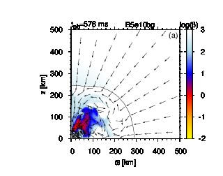
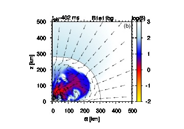
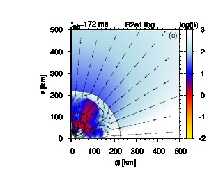
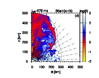
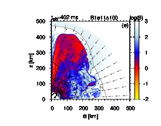
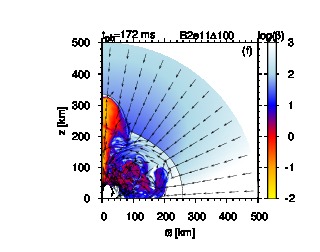
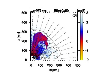
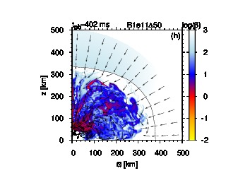
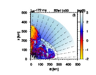
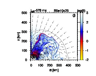
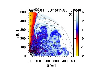
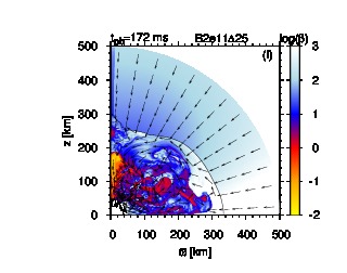
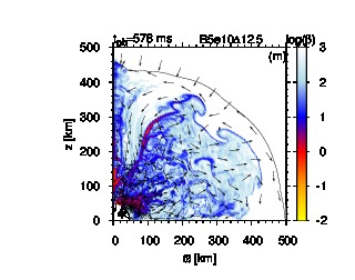
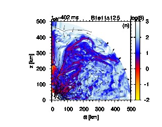
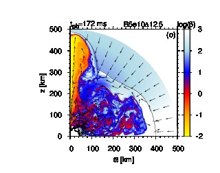
Figure 8.— Color maps of the plasma beta with velocity vectors presented by arrows at $t_{\textrm{pb}}=$578, 402, and 172 ms for model series B5e10, B1e11, B2e11, respectively.

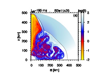
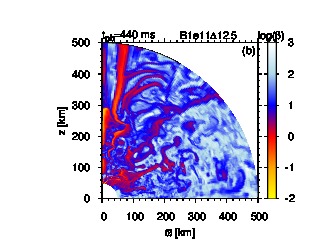
Figure 9.— Color maps of the plasma beta for model B2e11$\Delta$25 at $t_{\textrm{pb}}=$195 ms (a) and model B1e11$\Delta$12.5 at $t_{\textrm{pb}}=$440 ms (b), which are supplemental plots for panels (l) and (n) of Figure 8, respectively.

The dynamics change even more drastically when the spatial resolution is increased (MRI runs). Figure 8 displays the distributions of the plasma beta for all the 15 models at $t_{\textrm{pb}}=578$, 402, and 172 ms for model series B5e10 (left column), B1e11 (middle column), and B2e11 (right column), respectively. In model series B2e11, all the MRI runs result in the formation of a collimated low-$\beta$ jet emerging from inside the roughly-spherical shock, whereas the BG run yields an almost spherical expansion of the shock wave. Note that the low-$\beta$ region seen in panel (l) for model B2e11$\Delta$25 at 172 ms evolves into a collimated jet later on as shown in panel (a) of Figure 9. Meanwhile, in a weaker-field model series B1e11, the situation is not as simple as in model series B2e11. As the resolution gets higher from model B1e11bg to B1e11$\Delta$100, the shape of shock surface changes from spherical to prolate, but it returns to spherical shape when the resolution is doubled again (see panels (b), (e), (h) of Figure 8). Another doubling of the resolution, in turn, brings about the formation of a collimated low-$\beta$ jet emerging from inside the spherical shock (model B1e11$\Delta$25, panel (k)). In the highest resolution model B1e11$\Delta$12.5, a low-$\beta$ region is observed around the radius of 200 km in the vicinity of the pole (panel (n) of Figure 8), which may hint at a later jet formation. Although the head of low-$\beta$ region is still lingering around the radius of 300 km at the end of the simulation ($t_{\textrm{pb}}=$440 ms, see panel (b) of Figure 9), we expect that it would propagate further and eventually forms a collimated jet as found in model B1e11$\Delta$25 (see below). Finally in the weakest-field model series B5e10, the shock surfaces are roughly spherical for all the resolutions except model B5e10$\Delta$100, which has a prolate shock, and no model shows a jet formation until the end of the simulation.

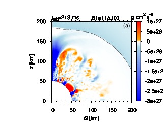
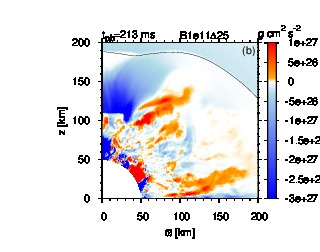
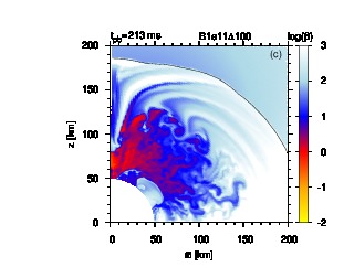
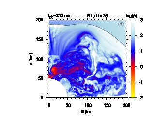
Figure 10.— Color maps of the ram pressure (upper panels) and the plasma beta (lower panels) for model B1e11$\Delta$100 (left panels) and B1e11$\Delta$25 (right panels). The ram pressure is multiplied by $-1$ where the radial velocity is negative.

We first discuss the factors responsible for the different shock morphorogies for different resolutions by comparing models B1e11$\Delta$100 and B1e11$\Delta$25 at $t_{\textrm{pb}}=213$ ms, several milliseconds prior to the launch of the collimated-jet in model B1e11$\Delta$25. The upper panels of Figure 10 depict the distribution of the ram pressure for the two models. It is observed in both the models that a vicinity of the pole is dominated by intense downflow (blue region), outside of which modest outflow driven by relatively-low plasma beta is seen (red region; see also lower panels). The width of the downflow channel is found to be narrower for the lower resolution model B1e11$\Delta$100, which would be due to less effective MRI: the better the MRI resolved, the more efficiently angular momentum is transferred outwards from the rotation axis, with which the rotational support decreases further around the pole and a broader downflow channel forms. Accordingly, the lower-$\theta$ edge of the outflow gets closer to the pole in this model, viz. the matter is ejected more preferentially along the pole. It is likely that this causes the prolate shock surface found in a model B1e11$\Delta$100. Note that although relatively-low plasma beta, $\beta\sim 1$, is seen around the bottom of the downflow channel in both the models, it seems not enough to drive the matter outward against the downflow (see the lower panels of Figure 10). The magnetically-driven mass ejection is only possible for the region outside the channel with such relatively-low plasma beta. It is found from Figure 8 that the trend of broader downflow channel and thus a larger deflection of the outflow direction from the pole for higher resolution models is valid for a wide range of resolution in model-series B5e10 and B1e11 as long as a jet is absent. This suggest that our interpretation for the shock morphology is reasonable. Note that the trend discussed here becomes no longer valid once a jet appears, since it changes the flow structure.

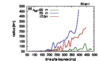
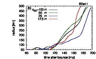
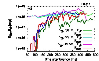
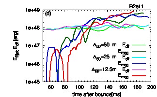
Figure 11.— Evolution of low-$\beta$ head (upper panels), and the downflow energy, $E_{\textrm{df}}$ and magnetic energy responsible for jet driving, $E_{B_{\textrm{jet}}}$ (lower panels). The left and right columns are for models series B1e11 and B2e11, respectively. Note that the time average over the interval of 10 ms is taken for each plot.

According to the above discussion, the collimated-jets seen in some models must have been launched against the downflow. In the case of model B1e11$\Delta$25, the low-$\beta$ clump around $r=70$ km in the vicinity of the pole observed in panel (d) of Figure 10 is a prototype of the low-$\beta$ jet seen at a later phase (panel (k) of Figure 8). We found indeed that this low-$\beta$ clump suffers from successive depression by the downflow until it finally forms the collimated jet.

To see the process of jet formation more in detail, we define the “low-$\beta$ head” by the maximum radius of the region where the ratio of the matter pressure to magnetic pressure, each of which is angularly averaged over $\theta\leq 5^{\circ}$, is less than 0.5, and plot the evolutions of them for model series B1e11 and B2e11 (see the upper panels of Figure 11). For model B1e11$\Delta$25 the sequence of the depression described above is clearly seen as an oscillatory evolution of the low-$\beta$ head until $t_{\textrm{pb}}\approx 370$ ms, from which it grows monotonically. Model B1e11$\Delta$12.5 shows a slower growth of the low-$\beta$ head and more distinct feature of oscillation, indicating that the depression by downflow is more significant. A similar oscillation is also found for model B1e11$\Delta$100, but the low-$\beta$ head almost stagnates at a small radius in this case. On the contrary to the weaker field case, model series B2e11 shows no oscillation of the low-$\beta$ head, which grows almost monotonically in all of the three models plotted in panel (b) of Figure 11.

From the above discussion, the downflow seems the key to the propagation of low-$\beta$ head and the eventual formation of a collimated jet. Then the condition for the jet formation may be obtained by comparing the kinetic energy of the downflow and the magnetic energy responsible for the jet driving. As argued below, we indeed found that this comparison reasonably explains the jet formation.

In the lower panels of Figure 11 we plot the time evolutions of the above two energies for model series B1e11 and B2e11, defining the former as $E_{\textrm{df}}\equiv\int_{v_{r}<0}(\rho v_{r}^{2}/2)dV$ and the latter as $E_{B_{\textrm{jet}}}\equiv\int_{\beta<0.5}(B^{2}/8\pi)dV$, where the integrants are nonzero only for $v_{r}<0$ and $\beta<0.5$, respectively, and the integration ranges are confined to 50 km$\leq r\leq r_{\textrm{sh}}$ and $\theta<20^{\circ}$. In model series B2e11, the evolutions of $E_{B_{\textrm{jet}}}$ appears rather similar among the different resolutions. In each model, $E_{B_{\textrm{jet}}}$ exceeds $E_{\textrm{df}}$ around $t_{\textrm{pb}}\approx 100$ ms, which is found to approximately coincide with the start of the low-$\beta$ head propagation (see right column of Figure 11). This suggests that the $E_{\textrm{df}}$-$E_{B_{\textrm{jet}}}$ comparison is indeed a rough indicator for the jet formation.

Unlike in model series B2e11, the values of $E_{B_{\textrm{jet}}}$ in model series B1e11 rather diverge among different resolutions during a late phase after their growth nearly saturates around $t_{\textrm{pb}}\approx 250$ ms. Interestingly, while reducing the grid size, $\Delta_{50}$, from 50 m to 25 m result in averagely-larger $E_{B_{\textrm{jet}}}$ during the late phase, which may be simply due to smaller numerical diffusivity, another doubling of resolution decreases that value (see panel (c) of Figure 11). We infer that the decrease of $E_{B_{\textrm{jet}}}$ observed here is caused by the interaction of low-$\beta$ matter with downflow. Since the downflow matter involves high-$\beta$ (see Figure 10), the plasma beta of low-$\beta$ matter increases as it hit by and mixed with the downflow matter, which results in downturn of $E_{B_{\textrm{jet}}}$. Indeed, the panel (c) of Figure 11 shows that the downflow energy, $E_{\textrm{df}}$, is averagely larger in model B1e11$\Delta$25 than in B1e11$\Delta$12.5, which is due to more effective MRI as discussed before, and the effect of downflow is expected to be more standout for the latter model. Although the effect of the downflow basically becomes more potent by increasing the resolution, whether it is essential for the change of $E_{B_{\textrm{jet}}}$ would depend on the competition with other factors. For the increase of $E_{B_{\textrm{jet}}}$ from model B1e11$\Delta$50 to B1e11$\Delta$25, it is likely that the reduction of the numerical diffusivity is more important than the increment of the downflow effect. Meanwhile, the fact that the $E_{B_{\textrm{jet}}}$ is roughly unchanged by increasing the resolution in model series B2e11 indicates that the downflow effect is insignificant in these models. One reason for this would be that the plasma beta of low-$\beta$ matter is low enough to maintain $\beta<0.5$, the criterion for adding up $E_{B_{\textrm{jet}}}$, even after the mixing with downflow matter. We compare in Figure 12 the $\beta$-distribution of magnetic energy contained within $\theta<20^{\circ}$ for models B1e11$\Delta$12.5 and B2e11$\Delta$12.5 at the moment when $E_{\textrm{df}}$ first reaches $2.0\times 10^{48}$ erg in each model, and found that the latter model indeed involves more low-$\beta$ matter. Another reason that we consider important is that models B2e11 take shorter time to reach the saturation of magnetic energy than models B1e11 do (see Figure 4 and lower panels of Figure 11). Since $E_{\textrm{df}}$ gradually increases until attenuated by the jet formation, an early growth of magnetic energy is advantageous to alleviate the downflow effect. In fact, the value of $E_{\textrm{df}}$ at the moment when it is caught up with by $E_{B_{\textrm{jet}}}$, is generally smaller in model series B2e11 ($E_{\textrm{df}}=0.6-1.2\times 10^{48}$ erg) than in B1e11 ($E_{\textrm{df}}=1.5-2.3\times 10^{48}$ erg).

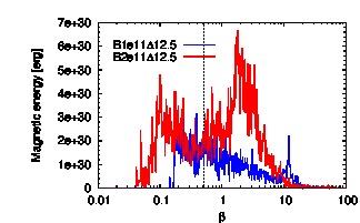
Figure 12.— $\beta$-distribution of magnetic energy contained within $\theta<20^{\circ}$ for models B1e11$\Delta$12.5 and B2e11$\Delta$12.5 at the moment when $E_{\textrm{df}}$ first reaches $2.0\times 10^{48}$ erg in each model, $t_{\textrm{pb}}=198$ ms for the former and $t_{\textrm{pb}}=140$ ms for the latter. The vertical-dotted line represents $\beta=0.5$.

Bearing in mind the variations of $E_{B_{\textrm{jet}}}$ and $E_{\textrm{df}}$ among the different resolutions mentioned for model series B1e11 in the above, the non-monotonic dependence of jet formation on the resolution found in these models (the middle column of Figure 8) is also explained reasonably in terms of the $E_{\textrm{df}}$-$E_{B_{\textrm{jet}}}$ comparison. For model B1e11$\Delta$50, the fact that $E_{B_{\textrm{jet}}}$ is almost always smaller than $E_{\textrm{df}}$ is consistent with the stagnation of the low-$\beta$ head at small radii. Similar to model series B2e11, model B1e11$\Delta$25 shows the outward propagation of the low-$\beta$ head after $E_{B_{\textrm{jet}}}$ becomes comparable to $E_{\textrm{df}}$ around $t_{\textrm{pb}}\approx 220$ ms. Contrary to the former cases, however, $E_{B_{\textrm{jet}}}$ does not exceed $E_{\textrm{df}}$ so much and sometimes even falls behind that, as expected from the oscillatory evolution of the low-$\beta$ head. In the higher resolution model B1e11$\Delta$12.5, the low-$\beta$ head starts to propagate after $E_{B_{\textrm{jet}}}$ grows comparable to $E_{\textrm{df}}$ around $t_{\textrm{pb}}\approx 280$ ms, but shows remarkable oscillations as $E_{B_{\textrm{jet}}}$ occasionally becomes smaller than $E_{\textrm{df}}$ by up to factor $\approx 10$, due to the downflow effect. About 140 ms later, however, low-$\beta$ filaments outside the downflow choke the channel region (see panel (b) of Figure 9), decreasing $E_{\textrm{df}}$ drastically and resulting in the acceleration of the low-$\beta$ head. As mentioned before the position of the low-$\beta$ head is still at $r<300$ km and no clear jet formation is observed by the end of the simulation. Nevertheless, since $E_{B_{\textrm{jet}}}$ exceeds $E_{\textrm{df}}$ by almost factor 10 at that time, and the latter does not increase significantly afterward, we expect that a collimated jet will form later also in model B1e11$\Delta$12.5. It should be noted that since doubling the resolution from model B1e11$\Delta$25 to B1e11$\Delta$12.5 renders the downflow effect more significant, which is disadvantageous for a jet formation, higher resolution runs are necessary to understand how the dynamics converge in terms of resolution for model series B1e11.

Since the jet formations discussed above take place close to the pole, where the coordinates become singular, one may be worried that the observed features are merely numerical artifacts. Although some level of numerical noises originating from the coordinate singularity may be inevitable in spite of the special treatment described in Section 2, we believe that they are of physical origin. This is because the jet is born at some distance from the pole, $\approx 10$ km (panel (d) of Figure 10), which is much larger than the width of the region of the special treatment, and because the evolution of the low-$\beta$ region is reasonably understood by the above arguments.

3.2.3 Boost of Explosion via MRI

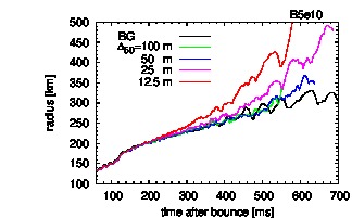
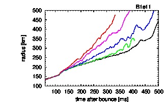
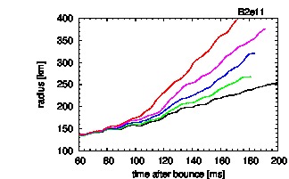
Figure 13.— Time evolutions of the shock radii at equator for all the models.

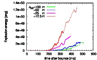
Figure 14.— Time evolutions of the diagnostic explosion energies for model series B1e11. After the maximum shock position exceeds the outer radial boundary, they are plotted by dotted lines.

Although the variation of dynamical behavior with the resolution seems rather complicated as described above, there is actually one clear trend, i.e., the faster shock expansion at the equator for the higher-resolutions (see Figure 8 and 13). Since the equatorial region contains a larger amount of mass compared to the polar region, the larger explosion energy is expected for the faster shock expansion. As shown shortly, this is indeed the case.

Figure 14 shows the time evolution of the diagnostic explosion energy, which is defined as the sum of the kinetic, magnetic, internal, and gravitational energies over the fluid elements that move outward with positive energies, for model series B1e11. This clearly shows that the diagnostic explosion energy becomes larger as the resolution is increased. Figure 8 indicates that the magnetic effects are not necessarily lager for higher resolutions (e.g., compare panel (e) and (h)), which suggests that the magnetic pressure is not a key factor to boost the explosion. Note that although the collimated jets are driven by magnetic pressure, they give a minor contribution to the explosion energy due to their small volumes. As pointed out by Sawai & Yamada (2014), the increase in the explosion energy is attributes to the more efficient neutrino heating in higher resolution models.

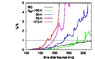
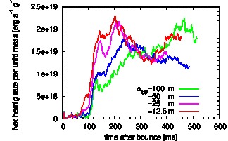
Figure 15.— Time evolutions of $\tau_{\textrm{a}}/\tau_{\textrm{h}}$ (upper panel) and the net heating rate per unit mass averaged over the heating region (lower panel) for model series B1e11. See text for the definition of $\tau_{\textrm{a}}$ and $\tau_{\textrm{h}}$.

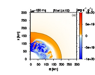
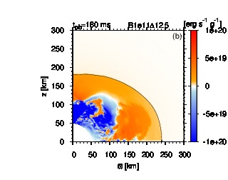
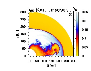
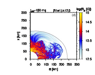
Figure 16.— Top panels: color maps for the net heating rate per unit mass for models B1e11$\Delta$100 (panel (a)) and B1e11$\Delta$12.5 (panel (b)) at $t_{\textrm{pb}}=180$ ms. Panel (c): Color map for the proton fraction, $Y_{p}$, for model B1e11$\Delta$12.5. Panel (d): Color map for the strength of the poloidal magnetic fields for model B1e11$\Delta$12.5.

How close to revival the stalled shock is roughly measured by the ratio of the advection timescale, $\tau_{\textrm{a}}$, during which matter traverses the gain region, to the heating timescale, $\tau_{\textrm{h}}$, within which matter gains enough energy to overcome gravity (Thompson, 2000). Following Dolence et al. (2013), we define the advection timescale as

$$\tau_{\textrm{a}}=\int^{R_{\textrm{gain}}}_{R_{\textrm{sh}}}\frac{dr}{\langle\langle v_{r}\rangle\rangle},$$ (31)

where the double angle bracket implies that the solid-angle average over $4\pi$ as well as the time average over the interval of 10 ms are taken. $R_{\textrm{sh}}$ is the mean shock radius, whereas $R_{\textrm{gain}}$ is defined as the innermost radius at which the solid-angle-averaged net heating is positive. The heating timescale is defined as

$$\tau_{\textrm{h}}=\frac{4\pi\int^{R_{\textrm{gain}}}_{R_{\textrm{sh}}}\langle e+\frac{\rho v^{2}}{2}+\frac{B^{2}}{8\pi}+\rho\Phi\rangle r^{2}dr}{4\pi\int^{R_{\textrm{gain}}}_{R_{\textrm{sh}}}\langle Q_{E}^{\textrm{em}}+Q_{E}^{\textrm{abs}}\rangle r^{2}dr},$$ (32)

where the single angle brackets mean that the only solid-angle average is taken. The upper panel of Figure 15 plots the evolution of $\tau_{\textrm{a}}/\tau_{\textrm{h}}$ for model series B1e11. The comparison of this figure with Figure 14 indicates that shock revival, which is indicated by positive explosion energies, roughly corresponds to $\tau_{\textrm{a}}/\tau_{\textrm{h}}\gtrsim 1$. It is also evident that higher resolutions result in higher heating efficiency.

In Sawai & Yamada (2014), we argued that this is due to the increase of $\tau_{\textrm{a}}$ in the higher resolution models as a result of more efficient angular momentum transfer, which leads to the expansion of the heating region. This is true of the current models. Comparison between models B1e11$\Delta$100 and B1e11$\Delta$12.5 at $t_{\textrm{pb}}=180$ ms shows that the heating region is thicker (see the upper panels of Figure 16) and the amount of angular momentum contained in the heating region is larger for the latter model: they are $7.0\times 10^{47}$g cm²s^-1 for model B1e11$\Delta$100 and $1.9\times 10^{48}$g cm²s^-1 for model B1e11$\Delta$12.5 at $t_{\textrm{pb}}=180$ ms.

Besides the increment of $\tau_{\textrm{a}}$, we found in this paper that the reduction of $\tau_{\textrm{h}}$ owing to a larger heating rate per unit mass is also contributing to the larger $\tau_{\textrm{a}}/\tau_{\textrm{h}}$ in the higher resolution models. As shown in the lower panel of Figure 15, the heating rate per unit mass during $\sim 100$–$250$ ms, the period crucial to shock revival, becomes larger as the resolution increases. The comparison of the upper panels of Figure 16 for models B1e11$\Delta$100 and B1e11$\Delta$12.5 indicates that this is originated in a patch of region with large heating rates around the equator observed in the latter model. We evaluated the heating and cooling rates separately and found that the relatively inefficient cooling in the patch compared with the surroundings is responsible for the larger net heating rate. From Equation (9), the cooling rate per unit mass, $Q_{E}^{\textrm{em}}/\rho$, is proportional to $(kT)^{6}$ and $Y_{n}\mathcal{F}_{5}(-\eta_{e})+Y_{p}\mathcal{F}_{5}(\eta_{e})$. We found that there is no substantial difference in $(kT)^{6}$ between the patch and surroundings but that $Y_{n}\mathcal{F}_{5}(-\eta_{e})+Y_{p}\mathcal{F}_{5}(\eta_{e})$ is several times smaller in the patch. In the surroundings, where $Y_{n}\sim Y_{p}\sim 0.2$, $\mathcal{F}_{5}(-\eta_{e})\sim 10$, and $\mathcal{F}_{5}(\eta_{e})\sim 900$, the products are $Y_{n}\mathcal{F}_{5}(-\eta_{e})\sim 2$ and $Y_{p}\mathcal{F}_{5}(\eta_{e})\sim 200$, viz., the cooling is dominated by electron capture since electrons are much more abundant than positrons. On the other hand, the electron capture is found to be relatively inactive in the patch due to small number of protons ($Y_{p}\sim 0.05$, see panel (c) of Figure 16) and electrons ($\mathcal{F}_{5}(\eta_{e})\sim 500$): the product is $Y_{p}\mathcal{F}_{5}(\eta_{e})\sim 30$. We found that the positron capture rate is small as well in the patch: $Y_{n}\mathcal{F}_{5}(-\eta_{e})\sim 20$, where $Y_{n}\sim 0.8$ and $\mathcal{F}_{5}(-\eta_{e})\sim 30$. To summarize, the the larger heating rate in the patch is caused by poverty of protons and electrons, and a low electron capture rate as a consequence.

The low-$Y_{p}$ (equivalently low-$Y_{e}$) region coincides with the location where the poloidal magnetic field is relatively strong (compare panels (c) and (d) of Figure 16). This suggests that low-$Y_{p}$ fluids originally located at small radii are drifted along the magnetic flux loops by MRI. We also found that the outflow along the rotation axis observed in model B1e11$\Delta$100 and the collimated jets found in models B1e11$\Delta$25 and B1e11$\Delta$12.5 (see panels (e), (k), and (n) of Figure 8, respectively) also convey low-$Y_{p}$ matter from deep inside the core, which is reflected to the rise of the volume-averaged net heating rate seen after $t_{\textrm{pb}}\sim 350$ ms for these models (see green, magenta, and red lines in the bottom panel of Figure 15).

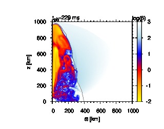
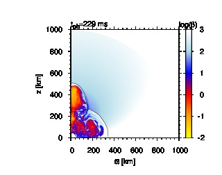
Figure 17.— Color maps for the plasma beta for models B2e11H (upper panel) and B2e11NH (lower panel) at $t_{\textrm{pb}}=229$ ms.

In order to estimate the possible influences of these effects on the global dynamics, we carried out two groups of additional test simulations based on models B1e11$\Delta$50 and B2e11$\Delta$50. The first one of them are extends the radial outer boundaries to $r=1000$ km (models B1e11H and B2e11H). The other one is different in that the net neutrino heating is switched off, i.e., $Q_{E}^{\textrm{abs}}+Q_{E}^{\textrm{em}}=\max\left[Q_{E}^{\textrm{abs}}+Q_{E}^{\textrm{em}},0\right]$ (models B1e11NH and B2e11NH).

Figure 17 shows the profile of the plasma beta for models B2e11H and B2e11NH at $t_{\textrm{pb}}=229$ ms, when the shock surface reaches $r=1000$ km in model B2e11H. Comparing the two panels, we can immediately see the importance of the neutrino heating: when the shock surface reaches $r=1000$ km in model B2e11H, that in model B2e11NH has just passed the radius of 500 km, and it arrives at $r=1000$ km 65 ms later than model B2e11H. Even though the collimated jets observed in these two models are magnetically dominated, the neutrino heating plays a significant role. The diagnostic explosion energies at the time when the shock fronts reach the radius of 1000 km are $4.6\times 10^{49}$ and $1.8\times 10^{49}$ erg, respectively, for models B2e11H and B2e11NH, implying that the contribution of the neutrino heating to the explosion energy is about 60%. The neutrino heating is even more crucial for weaker initial fields. The shock surface in model B1e11NH stays within 400 km even at 678 ms after bounce while that of B1e11H has passed the radius of 1000 km at $t_{\textrm{pb}}=595$ ms. The diagnostic explosion energy in model B1e11H is $4.7\times 10^{49}$ erg at the time when the shock front reach the radius of 1000 km, while that in model B1e11NH is negligibly small, $\lesssim 2\times 10^{47}$ erg, through the simulation. Note that longer time simulations following the propagation of the shock front through the whole progenitor would be necessary to correctly measure the explosion energy.

The small contribution of magnetic field to the explosion energy discussed above is a substantial difference from previous MHD simulations involving magnetar-class initial fields, in which a magnetic field alone boosts the explosion energy up to $\sim 10^{51}$ erg, accompanying a jet with a rather-large opening angle (e.g., Yamada & Sawai, 2004). This implies that in our models, the Maxwell stress is weaker, and thus the extraction of the rotational energy is less efficient than in those simulations.

3.3. Effects of Inner Boundary

We have seen that the MRI efficiently amplifies weak seed magnetic fields to dynamically important strengths, having a positive impacts on explosion. In this section, we investigate whether the above results depends on the location of the inner boundary, shifting it to smaller radii in model B2e11$\Delta$50.

We ran a new simulation with the inner boundary at $r=30$ km to take the effect of strong differential rotation beneath the radius of 50 km into account, which we refer to as model Rin30. The spatial resolution of this model is similar to that of model B2e11$\Delta$50 outside the radius of 50 km and is 30 m at the inner boundary. The fraction of the volume where $N_{\textrm{MRI}}$ is less than 10 is only a few percent inside the radius of 50 km, which is similar to that outside (see Figure 2).

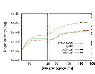
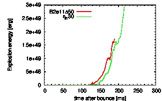
Figure 18.— Upper panel: time evolutions of the magnetic energies contained in the range of $50<(r/$km$)<500$ for models Rin30 and B2e11$\Delta$50. Lower panel: time evolutions of the diagnostic explosion energies for models Rin30 and B2e11$\Delta$50. After the maximum shock position exceeds the outer radial boundary, they are plotted by dotted lines.

The growth rates of MRI inside the radius of 50 km are found to be lager than those outside on average. The upper panel of Figure 18 indicates that the exponential growth rate of $E_{B_{p}}$ averaged over the range of $50<(r/$km$)<500$ is larger for model Rin30 than for model B2e11$\Delta$50. This implies that the magnetic fields amplified inside the radius of 50 km are advected outward in model Rin30. Note that the degree of differential rotation is even greater inside the radius of 30 km, and thus the above effect would be more pronounced if we carried out the simulation with a yet smaller radius of inner boundary. On the other hand, we found that the saturation level of $E_{B_{p}}$ is unaffected by the position of the inner boundary, which may be reasonable if the saturation is determined by the strength of the numerical diffusion, and hence the spatial resolution, which are more or less the same (see Section 3.1). The evolution of $E_{B_{t}}$ is similar to that of $E_{B_{p}}$.

The global dynamics does not change significantly, either, by moving the inner boundary position. The low-$\beta$ collimated jet that emerges from inside the roughly-spherical shock is a feature common to both models B2e11$\Delta$50 and Rin30. Whereas the evolutions of the jets are rather different between the two models, the shock propagation on the equator are very similar between the two. As shown in the lower panel of Figure 18, the diagnostic explosion energies of the two models are also nearly identical. From these results, we believe that the conclusions of the current study are not affected by our choice of the inner boundary position, $r=50$ km.

4. Discussion and Conclusion

We have performed MHD simulations of the core-collapse of rapidly-rotating magnetized stars in two dimensions under axisymmetry, changing both the strength of magnetic field and the spatial resolution. Our goal is to study the behavior of the MRI in core-collapse supernovae and its impacts upon the global dynamics. As a result of computations we found the followings.

The MRI greatly amplifies the seed magnetic fields even in the dynamical background of the core-collapse. Although the dominant mode, buoyant mode or Alfvén mode, differs from location to location, the former plays a primary role in the exponential growth phase. It is true that the linear growth rate of the buoyant mode is independent of the wavelength, a certain degree of high spatial resolution seems necessary to correctly capture the exponential growth. The magnetic energies of the poloidal component gets nearly saturated within the simulation times in all models, where the saturation level is higher for larger initial magnetic fields. The magnetic energies of the toroidal component grow continuously in most of the models, on the other hand, and the core becomes toroidal-field dominant.

The MRI also has a grate impacts on the global dynamics. Models in which the MRI are well resolved show faster expansions of shock surface and obtain more powerful explosions. The formation of collimated jet is also found in models where the initial magnetic field is relatively strong and the MRI is well resolved. The following two effects are found to be the key to the boost of explosion: the first one is the expansion of the heating region due to the outward angular momentum transfer. This makes the advection timescale, or the time for matter to traverse the heating region, longer and thus enhance the heating; the second effect is the drift of low-$Y_{p}$ (equivalently low-$Y_{e}$) matter along the MRI-distorted magnetic flux loops as well as their ejection by the jets, from deep inside the core to the heating region. The cooling due to electron capture is reduced in the low-$Y_{p}$ region, and the net heating rises as a result.

The diagnostic explosion energies obtained in the current simulations are much smaller than the typical value of $\sim 10^{51}$ erg in reality. Note, however, that our choice of the neutrino luminosity, $L_{\nu_{e}}=L_{\bar{\nu_{e}}}=1.0\times 10^{52}$ erg s^-1, which is assumed to be constant, is quite modest. According to the core-collapse simulations by Bruenn et al. (2013), who employed the flux-limited diffusion with the ray-by-ray-plus approximation for neutrino transport, both $L_{\nu_{e}}$ and $L_{\bar{\nu_{e}}}$ are $\sim 5.0\times 10^{52}$ erg s^-1 at $t_{\textrm{pb}}\sim 100$ ms and decay to $\sim 1.0\times 10^{52}$ erg s^-1 over several hundred milliseconds. If such an evolution of luminosity is adopted in our simulations more energetic explosion would be obtained.

Although our choice of the initial magnetic field strength, $\sim 10^{11}$ G, is much smaller than those assumed in the former global MRI simulations (e.g., Obergaulinger et al., 2006; Shibata et al., 2006; Sawai et al., 2013a), most of progenitors of core-collapse supernovae may posses even weaker magnetic fields (Wade & the MiMeS Collaboration, 2014). Since lower saturation magnetic fields are expected for weaker initial magnetic fields according to our results, the impact of MRI in ”normal” supernovae will be smaller than that found in this work. Although it is important to study much weaker magnetic fields, simulations will be computationally expensive and thus currently unfeasible: a reduction of the initial magnetic field by half, with the spatial resolution kept at the current level, demands eight times higher computational cost for 2D time-explicit simulations.

The dependence on the initial rotation also needs to be investigated, since the rotation speed of stars is also likely to distribute over a wide range (Ramírez-Agudelo et al., 2013). We are currently undertaking such studies, and the results will be presented elsewhere in the future.

Although our simulations are 2D under axisymmetry, supernovae occur in three dimensions in reality, and non-axisymmetric effects such as dynamo, three-dimensional turbulence, non-axisymmetric modes of various instabilities may be important. One should keep in mind that these effects possibly alter results obtained by current 2D simulations. For example, 3D-MHD simulations performed by Mösta et al. (2014) demonstrated that magnetically driven-jets can be destroyed by the $m=1$ mode of a kink-type instability, whereas such destruction of the jet was not observed in 3D-MHD simulations by Mikami et al. (2008). In order to know how essential non-axisymmetric effects are, 3D global simulations are mandatory. During the reviewing process of this paper, Mösta et al. (2015) published the results of the first global-3D simulations of the MRI in proto-neutron stars. Under quadrant symmetry, they had simulated the evolution of the MRI for 10 ms, and found the formation of large-scale, strong toroidal fields, which hints at later magnetically-driven mass ejections. Such simulations have only just begun, and the possible 3D effects mentioned above should be studied in detail in the future. This requires long-term, large-domain, full 3D simulations, which may be marginally feasible with exa-flops computers of the next generation.

Masada et al. (2007) and Guilet et al. (2015) argued that the neutrino viscosity may hamper the growth of MRI deep inside the core, i.e., $r\lesssim 30$ km for a fast rotation like ours. Applying the magnetic field of $\sim 10^{13}$–$10^{14}$ G obtained in our BG runs for $r\lesssim 30$ km to the fast rotation model of Guilet et al. (2015), we found that the neutrino viscosity may be marginally important there. Since the inner boundary condition of our MRI runs is given by the data of the BG runs of low resolution, the artificial suppression of MRI by numerical diffusions may effectively mimic the damping by the neutrino viscosity. We hence believe that full-sphere simulations including the neutrino viscosity will not change our conclusions in this paper so much, if the viscous process is important at all.

References

- Akiyama et al. (2003) Akiyama, S., Wheeler, J. C., Meier, D. L., & Lichtenstadt, I. 2003, ApJ, 584, 954
- Balbus & Hawley (1991) Balbus, S. A., & Hawley, J. F. 1991, ApJ, 376, 214
- Balbus (1995) Balbus, S. A. 1995, ApJ, 453, 380
- Bruenn et al. (2013) Bruenn, S. W., Mezzacappa, A., Hix, W. R., et al. 2013, ApJ, 767, LL6
- Burrows et al. (2007) Burrows, A., Dessart, L., Livne, E., Ott, C. D., & Murphy, J. 2007, ApJ, 664, 416
- Dolence et al. (2013) Dolence, J. C., Burrows, A., Murphy, J. W., & Nordhaus, J. 2013, ApJ, 765, 110
- Endeve et al. (2010) Endeve, E., Cardall, C. Y., Budiardja, R. D., & Mezzacappa, A. 2010, ApJ, 713, 1219
- Endeve et al. (2012) Endeve, E., Cardall, C. Y., Budiardja, R. D., et al. 2012, ApJ, 751, 26
- Guilet et al. (2015) Guilet, J., Müller, E., & Janka, H.-T. 2015, MNRAS, 447, 3992
- Guilet Müller (2015) Guilet, J., Müller, E. 2015, MNRAS, 450, 2153
- Hanke et al. (2012) Hanke, F., Marek, A., Müller, B., & Janka, H.-T. 2012, ApJ, 755, 138
- Hawley et al. (1995) Hawley, J. F., Gammie, C. F., & Balbus, S. A. 1995, ApJ, 440, 742
- Iwakami et al. (2014) Iwakami, W., Nagakura, H., & Yamada, S. 2014, arXiv:1404.2646
- Janka (2001) Janka, H.-T. 2001, A&A, 368, 527
- Liebendörfer (2005) Liebendörfer, M. 2005, ApJ, 633, 1042
- McNally (1965) McNally, D. 1965, The Observatory, 85, 166
- Marek & Janka (2009) Marek, A., & Janka, H.-T. 2009, ApJ, 694, 664
- Masada et al. (2007) Masada, Y., Sano, T., & Shibata, K. 2007, ApJ, 655, 447
- Masada et al. (2015) Masada, Y., Takiwaki, T., & Kotake, K. 2015, ApJ, 798, LL22
- Masada et al. (2012) Masada, Y., Takiwaki, T., Kotake, K., & Sano, T. 2012, ApJ, 759, 110
- Mikami et al. (2008) Mikami, H., Sato, Y., Matsumoto, T., & Hanawa, T. 2008, ApJ, 683, 357
- Moiseenko et al. (2006) Moiseenko, S. G., Bisnovatyi-Kogan, G. S., & Ardeljan, N. V. 2006, MNRAS, 310, 501
- Mösta et al. (2015) Mösta, P., Ott, C. D., Radice, D., et al. 2015, Nature, doi:10.1038/nature15755
- Mösta et al. (2014) Mösta, P., Richers, S., Ott, C. D., et al. 2014, ApJ, 785, LL29
- Müller et al. (2012) Müller, B., Janka, H.-T., & Marek, A. 2012, ApJ, 756, 84
- Murphy et al. (2009) Murphy, J. W., Ott, C. D., & Burrows, A. 2009, ApJ, 707, 1173
- Nakamura et al. (2014) Nakamura, K., Kuroda, T., Takiwaki, T., & Kotake, K. 2014, arXiv:1403.7290
- Nordhaus et al. (2010) Nordhaus, J., Burrows, A., Almgren, A., & Bell, J. 2010, ApJ, 720, 694
- Obergaulinger et al. (2006) Obergaulinger, M., Aloy, M. A., & Müller, E. 2006, A&A, 450, 1107
- Obergaulinger et al. (2009) Obergaulinger, M., Cerdá-Durán, P., Müller, E., & Aloy, M. A. 2009, A&A, 498, 241
- Obergaulinger et al. (2014) Obergaulinger, M., Janka, H.-T., & Aloy, M. A. 2014, MNRAS, 445, 3169