Pattern formation in active particle systems due to competing alignment interactions

Abstract

Recently, we proposed a self-propelled particle model with competing alignment interactions: nearby particles tend to align their velocities whereas they anti-align their direction of motion with particles which are further away [R. Großmann et al., Phys. Rev. Lett. 113, 258104 (2014)]. Here, we extend our previous numerical analysis of the high density regime considering low particle densities too. We report on the emergence of various macroscopic patterns such as vortex arrays, mesoscale turbulence as well as the formation of polar clusters, polar bands and nematically ordered states. Furthermore, we study analytically the instabilities leading to pattern formation in mean-field approximation. We argue that these instabilities are well described by a reduced set of hydrodynamic equations in the limit of high density.

1 Introduction

The study of active matter is one of the main topics in modern classical statistical mechanics toner_hydrodynamics_2005 ; romanczuk_active_2012 ; vicsek_collective_2012 ; marchetti_hydrodynamics_2013 ; menzel_tuned_2015 . Active matter systems are composed of self-driven entities, so called active particles, which take up energy from their environment in order to move actively in a dissipative medium romanczuk_active_2012 . Due to the complex interplay of self-propulsion and dissipation, the dynamics of active matter systems is inherently out of thermodynamic equilibrium. Thus, complex spatio-temporal patterns may emerge in interacting active particle systems. There are numerous experimental realizations of active matter, for example driven filaments on the molecular scale schaller_polar_2010 , colloidal systems theurkauff_dynamic_2012 ; pohl_dynamic_2014 , bacterial colonies czirok_formation_1996 ; sokolov_concentration_2007 ; peruani_collective_2012 ; dombrowski_self-concentration_2004 ; sokolov_enhanced_2009 ; cisneros_fluid_2010 ; wensink_meso-scale_2012 ; zhang_swarming_2009 ; liu_multifractal_2012 as well as macroscopic systems like flocking birds ballerini_interaction_2008 and schooling fish katz_inferring_2011 .

The experimental study of bacterial colonies has become increasingly important for the understanding of active matter. On the one hand, the quantitative analysis of fascinating phenomena like clustering peruani_collective_2012 and vortex formation sumino_large-scale_2012 provide an excellent opportunity to test theoretical predictions, and, on the other hand, experiments often reveal unforeseen novel phases of active matter. Recently, a number of experiments reported the emergence of dynamic vortex patterns in dense suspensions of Bacillus subtilis dombrowski_self-concentration_2004 ; sokolov_enhanced_2009 ; cisneros_fluid_2010 ; wensink_meso-scale_2012 , Paenibacillus dendritiformis zhang_swarming_2009 as well as Escherichia coli liu_multifractal_2012 . In particular, it was observed that bacteria locally align their body axis. However, dynamic vortices (defects) in the velocity field appeared at larger scales. Interestingly, vortices are separated by a characteristic length scale which is larger than the size of an individual bacterium but smaller than the system size. This novel phenomenon was termed mesoscale turbulence.

Mesoscale turbulence was suggested to be described by a phenomenological hydrodynamic theory wensink_meso-scale_2012 ; dunkel_fluid_2013 which is a combination of both, the incompressible Toner-Tu theory for flocks toner_reanalysis_2012 ; chen_critical_2014 and the Swift-Hohenberg model Swift_hydrodynamic_1977 . The Swift-Hohenberg equation describes instabilities at finite wavelengths whereas the Toner-Tu theory is the basis for the description of flocking phenomena. A combination of both – a Turing instability in the velocity field together with convective particle transport – is sufficient to explain the pattern formation observed in bacterial suspensions dunkel_fluid_2013 . In particular, the experimentally observed velocity correlation function was reproduced by this hydrodynamic theory. However, the transport coefficients in the phenomenological model remain unknown constants.

In order to gain a deeper understanding of this pattern formation process, a particle based model was suggested by us grossmann_vortex_2014 . In this model, particles interact via competing velocity-alignment mechanisms: nearby particles tend to align their velocities whereas they anti-align their direction of motion with particles which are further away. The idea of competing interactions goes back to Turing turing_chemical_1952 who showed that instabilities on finite length scales arise in chemical systems due to the interplay of two competing species: a slowly diffusing activator and an inhibitor which diffuses fast compared to the activator. Within our active particle system, activation refers to the creation of local polar order by velocity-alignment which is inhibited by an opposing effect acting on larger length scales (anti-alignment). Similar types of competing interactions were studied in the context of spin models (ferromagnetic coupling to nearest neighbors vs. anti-ferromagnetic interaction with next-nearest neighbors krinsky_ising_1977 ; barber_non_1979 ; oitmaa_square_1981 ) and the Kuramoto model for synchronization (conformists vs. contrarians hong_kuramoto_2011 ). However, note that – in contrast to these examples – the competing alignment interaction in our model leads to instabilities of the velocity field which is, in turn, related to convective mass transport resulting in numerous novel pattern formation phenomena grossmann_vortex_2014 .

Generally, velocity-alignment interactions are understood as simple models for the interplay of various physical forces such as steric repulsion or hydrodynamics. The simplest active particle model with velocity-alignment interaction is the seminal Vicsek model vicsek_novel_1995 : particles move in continuous space at a constant speed and align their direction of motion with the local mean velocity plus some deviations (noise) in discrete time steps. Over the years, numerous modifications of the original Vicsek model were discussed (see e.g. chate_modeling_2008 ). In some studies, anti-alignment was included in different ways: for example, Menzel considered anti-alignment between two different particle populations menzel_collective_2012 , whereas Lobaskin et al. studied a model where particles do only align if their velocity are already aligned to a certain degree lobaskin_collective_2013 . For an overview on pattern formation in self-propelled particle systems, we refer the interested reader to a number of comprehensive review articles vicsek_collective_2012 ; romanczuk_active_2012 ; marchetti_hydrodynamics_2013 ; menzel_tuned_2015 .

In this work, we address the following questions. In section 2, we introduce our active particle model with competing alignment interaction in detail. In the subsequent section, we report the results of numerical simulations and discuss the collective dynamics exhibited by the system. Whereas we focused on the high density limit in grossmann_vortex_2014 , we study the phase space in detail including low and high densities here. In section 4, we derive hydrodynamic equations in the mean-field limit allowing us to understand the observed pattern formation qualitatively and to link our model to previously discussed phenomenological theories. Moreover, we estimate the quality of the approximations involved in the coarse-graining process and discuss their range of applicability.

2 Self-propelled particle model

We study an ensemble of $N$ interacting self-propelled particles (SPPs) in two spatial dimensions. We assume that particles move at constant speed which is justified if all processes related to the self-propulsion mechanism occur on negligibly small timescales. The generic dynamics of interacting SPPs is determined by the following set of stochastic differential equations

$$\frac{\mbox{d}\mathbf{r}_{i}(t)}{\mbox{d}t}\,=\begin{pmatrix}\cos\varphi_{i}\\ \sin\varphi_{i}\end{pmatrix}\!,\quad\frac{\mbox{d}\varphi_{i}(t)}{\mbox{d}t}=\sqrt{2D_{\varphi}}\,\xi_{i}(t)+\sum_{j\neq i}^{N}\mathfrak{f}_{\varphi}(\mathbf{r}_{ji},\varphi_{i},\varphi_{j}),$$ (1)

where we denote the spatial position of the $i$ths particle at time $t$ by $\vec{r}_{i}(t)$ and its direction of motion by $\varphi_{i}(t)$. The first term on the right-hand side of the angular dynamics represents noise indicating the random reorientation of particles due to spatial inhomogeneities or fluctuations of the driving force, whereas the second term accounts for binary interactions among the particles.

In the absence of inter-particle coupling, a SPP performs a persistent random walk: a particle moves ballistically at short timescales, whereas the motion is diffusive on large timescales due to angular fluctuations. The details of this diffusion process depend on the properties of the fluctuations mikhailov_self_1997 ; weber_active_2011 ; weber_active_2012 . Here, we consider the simplest case of Gaussian white noise with zero mean, $\left<\xi_{i}(t)\right>=0$, and temporal $\delta$-correlations: $\left<\xi_{i}(t)\xi_{j}(t^{\prime})\right>=\delta_{ij}\,\delta(t-t^{\prime})$. The parameter $D_{\varphi}$ parametrizes the intensity of the angular fluctuations.

The binary interaction $\mathfrak{f}_{\varphi}(\mathbf{r}_{ji},\varphi_{i},\varphi_{j})$ generally depends on the relative coordinate $\vec{r}_{ji}=\vec{r}_{j}-\vec{r}_{i}$ of the particles $i$ and $j$ as well as on their individual orientations. Here, we consider the interaction scheme proposed recently by the authors in grossmann_vortex_2014 including the following physical effects:

1. Due to the finite size of particles, these objects repel each other if they come closely together.
   $\Rightarrow$ short-range repulsion

2. In general, short-ranged anisotropic steric effects in combination with self-propulsion will lead to local orientational ordering. Here, we consider polar alignment:
   $\Rightarrow$ velocity-alignment

3. An active particle in a fluid or a polarly ordered cluster of swimming particles will induce hydrodynamic flows that in turn influence other particles. It has been shown for model swimmers that hydrodynamic interactions are generally anisotropic and may lead to velocity-alignment, anti-alignment or nematic alignment depending on the relative orientation and position of two swimmers as well as the swimming type (see e.g. baskaran_statistical_2009 ). Here, we replace the very complex hydrodynamic interaction and take one additional effective interaction mechanism into account:
   $\Rightarrow$ anti-velocity-alignment.

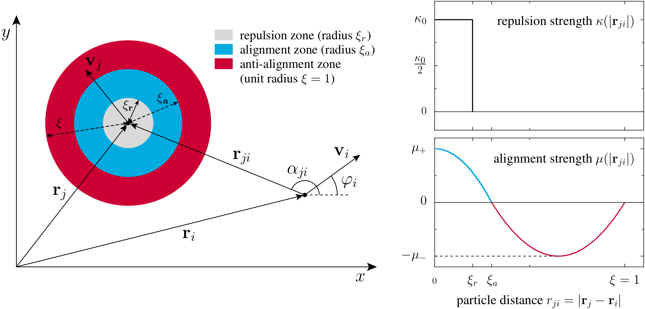
Figure 1: Visualization of geometric quantities and scheme of the pair-wise interaction.

We parametrize the binary interaction in (1) by

$$\mathfrak{f}_{\varphi}\!\left(\mathbf{r}_{ji},\varphi_{i},\varphi_{j}\right)=\kappa\!\left(\left|\mathbf{r}_{ji}\right|\right)\sin\left(\varphi_{i}-\alpha_{ji}\right)+\mu\!\left(\left|\mathbf{r}_{ji}\right|\right)\sin\left(\varphi_{j}-\varphi_{i}\right)\!.$$ (2)

The first term represents soft-core repulsion. The angle $\alpha_{ji}=\rm{arg}(\mathbf{r}_{ji})$ denotes the polar positional angle of particle $j$ in the frame of reference of particle $i$ (see also Fig. 1 for a graphical illustration). We assume a constant repulsion strength $\kappa_{0}$ for $\left|\mathbf{r}_{ji}\right|<\xi_{r}$ and vanishing repulsion otherwise: $\kappa\!\left(\left|\mathbf{r}_{ji}\right|\right)=\kappa_{0}\Theta(\xi_{r}-\left|\mathbf{r}_{ji}\right|)$.

The second term describes the competition of alignment and anti-alignment: For $\mu\!\left(\left|\mathbf{r}_{ji}\right|\right)>0$, particles tend to align their direction of motion whereas they anti-align in the opposite case. Throughout the paper, we will assume the following functional dependence of the alignment strength on distance

$$\mu\!\left(\left|\mathbf{r}_{ji}\right|\right)=\begin{cases}+\mu_{+}\,A_{+}\!\left(\left|\mathbf{r}_{ji}\right|\right)&0\leq\left|\mathbf{r}_{ji}\right|\leq\xi_{a},\\ -\mu_{-}\,A_{-}\!\left(\left|\mathbf{r}_{ji}\right|\right)&\xi_{a}\leq\left|\mathbf{r}_{ji}\right|\leq 1,\end{cases}$$ (3)

where $\mu_{+}$ and $\mu_{-}$ are positive constants. The distance dependence of the competing interactions is determined by the functions $A_{\pm}\!\left(\left|\mathbf{r}_{ji}\right|\right)$. We normalize the distance dependence such that $A_{\pm}\!\left(\left|\mathbf{r}_{ji}\right|\right)\in[0,1]$. Accordingly, $\mu_{+}$ and $\mu_{-}$ denote the maximal alignment and anti-alignment strength, respectively (cf. Fig. 1). Following grossmann_vortex_2014 , we use a piecewise quadratic distance dependence in this study:

$$A_{+}(r_{ji})=1-\left(\frac{r_{ji}}{\xi_{a}}\right)^{2},\quad A_{-}(r_{ji})=\frac{4(r_{ji}-\xi_{a})(1-r_{ji})}{(1-\xi_{a})^{2}}.$$ (4)

Note that the interaction described above is strictly short-ranged but nonlocal.

3 Simulation results - pattern formation and orientational order

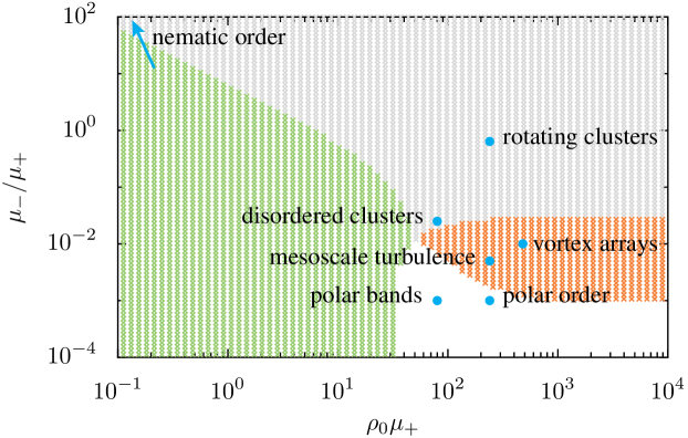
Figure 2: The figure shows the part of the parameter space which we study in this work. Points indicate the parameter values for which simulation results are shown (cf. Fig. 5 - Fig. 10). The background coloring (green, red, gray, white) was done in accordance with the predictions of the kinetic theory: in the green region, we expect the disordered (spatially homogeneous, isotropic) state to be stable; in the white area, we observe the emergence of polar order (local and global); in the gray and red colored part of the parameter space, we observe the emergence of patterns with a characteristic length scale (see section 4 for details).

In this section, we report on simulations of the microscopic dynamics for various parameters which were performed to obtain a general understanding of the collective dynamics and pattern formation exhibited by the system. Our simulations revealed that the system exhibits various types of spatio-temporal dynamics which we will discuss in the following.

We used the following fixed parameters in all simulations: repulsion range $\xi_{r}=0.1$, repulsion strength $\kappa_{0}=10$ and alignment range $\xi_{a}=0.2$. We focus our discussion on the variation of the alignment and anti-alignment strengths. The parameter values which we are going to discuss are represented in Fig. 2.

We go beyond our previous work grossmann_vortex_2014 and explore not only the high density regime ($\rho_{0}=150$) but also pattern formation at low densities ($\rho_{0}=20$). The studied density values may misleadingly appear as extremely large in comparison to the values typically studied in the Vicsek model vicsek_novel_1995 ; chate_collective_2008 . However, the alignment range is less than one ($\xi_{a}=0.2$) in our case. Hence, the mean number of particles within a box of edge length $\xi_{a}$ is $\left<n\right>=0.8$ for $\rho_{0}=20$ and $\left<n\right>=6$ for $\rho_{0}=150$. This is comparable to the regimes typically studied in the context of the Vicsek-model.

All simulations were performed using a rectangular domain with periodic boundary conditions with a linear size of $L=20=100\times\xi_{a}=200\times\xi_{r}$. This corresponds to a rather moderate system size with respect to the largest scale of interaction. We emphasize that the terms phase or state are therefore used here to describe stereotypical patters exhibited by the system at the corresponding mesoscale and shall not be confused with phases in the thermodynamic limit. Accordingly, global order refers here to the ordering of the entire simulated system and does not imply long-range order.

The initial conditions in all simulations were random positions and orientations of individual particles (disordered, homogeneous state). The simulation results were analyzed after the system had reached a stationary (dynamical) state, where no drift in order parameters and changes in patterns were observed anymore. The numerical time step was chosen sufficiently small to ensure numerical stability: $\Delta t\leq 5\cdot 10^{-3}$.

We measured polar and nematic orientational order using the corresponding order parameters

$$\Phi_{p}=\frac{1}{N}\left|\sum_{j=1}^{N}\,e^{i\varphi_{j}}\right|\!,\qquad\Phi_{n}=\frac{1}{N}\left|\sum_{j=1}^{N}\,e^{2i\varphi_{j}}\right|\!.$$ (5)

Furthermore, we calculated coarse-grained density $\rho_{c}(\vec{r},t)$ and velocity $\vec{v}_{c}(\vec{r},t)$ by binning of the particles positions and velocities on a rectangular grid with the coarse-graining scale set by the linear dimension of a grid cell: $dl=0.2$. Moreover, we calculated the momentum field via $\vec{w}_{c}(\vec{r},t)=\rho_{c}(\vec{r},t)\vec{v}_{c}(\vec{r},t)$. From the coarse grained fields, we deduced the two-point autocorrelation functions

$$C_{\rho\rho}(\vec{r})=\overline{\rho_{c}(\vec{r}^{\prime},t)\rho_{c}(\vec{r}^{\prime}+\vec{r},t)},\qquad{C_{ww}(\vec{r})=\overline{\vec{w}_{c}(\vec{r}^{\prime},t)\cdot\vec{w}_{c}(\vec{r}^{\prime}+\vec{r},t)}}$$ (6)

as well as their corresponding two-dimensional Fourier transforms $S_{\rho}(\vec{k})=\mathcal{F}[C_{\rho\rho}]$ and $S_{w}(\vec{k})=\mathcal{F}[C_{ww}]$. In Eq. (6), the overline indicates temporal averaging as well as averaging over the reference points $\vec{r}^{\prime}$.

3.1 Low density case ($\rho_{0}=20$)

In general, no orientational or spatial order can emerge if noise is dominant in comparison to the interaction strengths and, consequently, the system remains disordered, spatially homogeneous and isotropic.

In the limit of vanishing anti-alignment ($\mu_{-}=0$), the system reduces to a pure alignment model and the large-scale dynamics corresponds to the Vicsek model with the usual order-disorder transition from a disordered to a polarly ordered state at high alignment and small noise. In particular, we observe the emergence of large-scale travelling polar bands close to the order-disorder transition typical for Vicsek-type models chate_collective_2008 ; bertin_hydrodynamic_2009 . These structures can be clearly identified by the asymmetry of $C_{\rho\rho}$ and $C_{ww}$ reflecting an increased density and velocity autocorrelation perpendicular to the polar orientation and low-wavenumber peaks along the polar direction in both spectra $S_{\rho,w}$ (Fig. 5). Far away from the order-disorder transition (large $\mu_{+}$ and low $\mu_{-}$), the model exhibits the spatially homogeneous phase with polar order described and analyzed by Toner and Tu toner_reanalysis_2012 .

Small levels of anti-alignment do not destroy polar order at the system sizes studied. Only if $\mu_{-}$ is increased beyond a critical value, we observe the breakdown of global polar order. At low density, this breakdown is accompanied by the formation of small polar clusters, which are unstable and frequently break up. The corresponding density autocorrelation and its Fourier transform are rotationally symmetric and decay fast from a central peak indicating no long-ranged spatial structure. However, the ringlike structure of $C_{ww}$ and the maximum of $S_{w}(\vec{k})$ at a finite $|\vec{k}|$ identify a typical length scale of velocity correlations corresponding to the typical size of clusters (Fig. 5).

If the dynamics is dominated by anti-alignment (large $\mu_{-}$), we observe the formation of patches with nematic order where the polar clusters form lanes with neighboring lanes moving into opposite directions leading to global nematic order. This anti-parallel movement distinguishes these patters from the active crystals described in menzel_traveling_2013 ; menzel_active_2014 . $C_{\rho\rho}$ and $S_{\rho}$ show a high degree of spatial structure corresponding to the characteristic distance between clusters and lanes, respectively. Interestingly, the momentum autocorrelation function $C_{ww}$ also shows crystal like structure corresponding to a hexagonal lattice (Fig. 7). We emphasize that the autocorrelation functions were obtained from time-averaged density and momentum fields. In general, these autocorrelation functions and spectra will differ from ones obtained from a single snapshot at a fixed time $t$.

Surprisingly, the state with global nematic order and local polar order also emerges for anti-alignment only ($\mu_{+}=0$) as shown in Fig. 7. In this case, particles do not interact for distances $\xi_{r}\leq r_{ji}<\xi_{a}$ and local polar order is enforced by the strong anti-alignment at larger distance. The formation of the particular dynamic cluster state with dense polar clusters moving in lanes is the only possibility to ensure a stationary pattern when anti-alignment interaction is dominant. Nematic lanes were reported previously from other active matter systems (see e.g. helbing_freezing_2000 ; wensink_emergent_2012 ; mccandlish_spontaneous_2012 and menzel_tuned_2015 for a recent review as well as references therein), however not in absence of an (effective) alignment interaction and never with additional periodic order within individual lanes.

3.2 High density case ($\rho_{0}=150$)

We discussed simulation results in the high-density regime in grossmann_vortex_2014 . Here, we review these previous observations and go beyond by exploring a wider range of parameters. Snapshots of simulations in the high density regime are shown in Fig. 3.

Similar to the low-density case, we observe the emergence of large scale polar order for vanishing $\mu_{-}$. However, there are no bands due to the high density and we observe the Toner-Tu phase (Fig. 7). An increase in $\mu_{-}$ beyond a critical value leads to the breakdown of polar order. Just above this transition, we observe a dynamical regime without any spatial order but with a finite scale in the momentum field, which is reflected by a single ring of negative correlation about the central maximum of $C_{ww}$ and the rotationally symmetric $S_{w}$ with a maximum at finite $|{\bf k}|$. In contrast to the low-density case, we observe extended convective flows (jets) and transient vortices (Fig. 9) instead of diffuse clusters. This is the regime discussed in grossmann_vortex_2014 which reproduces qualitatively and quantitatively the observations of mesoscale turbulence in dense bacterial suspensions.

An increase in $\mu_{-}$ initially leads to the stabilization of the vortices and we observe the emergence of patches of spatially ordered vortex arrays arranged in a rectangular lattice with rather homogeneous density (Fig. 9). However, a further increase in $\mu_{-}$ leads also to growth of density inhomogeneities and eventually the rectangular vortex pattern transforms into a hexagonal array of rotating clusters (Fig. 10).

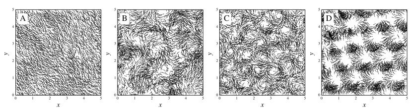
Figure 3: Close-up snapshots in the high density regime. From left to right: homogeneous polarly ordered state, mesoscale turbulence, rectangular vortex array, rotating clusters.

Figure 4: Polar bands ($\Phi_{p}=0.65$ and $\Phi_{n}=0.33$) at strong alignment $\mu_{+}=4$, weak anti-alignment $\mu_{-}=0.004$, low density $\rho_{0}=20$ and noise $D_{\varphi}=1.0$. (A) Global snapshot with particle positions shown by symbols and orientation indicated by the color according to the inset. (B) Zoom into a subregion of size $5\times 5$ with particle positions and orientations shown as vectors. (C) Time averaged density autocorrelation function $C_{\rho\rho}({\bf r})$ and (D) its Fourier transform $S_{\rho}({\bf k})$. (E) Time averaged momentum field autocorrelation function $C_{ww}({\bf r})$ and (F) its Fourier transform $S_{w}({\bf k})$.

Figure 5: Disordered clusters ($\Phi_{p}=0.021$ and $\Phi_{n}=0.020$) at strong alignment $\mu_{+}=4$, moderate anti-alignment $\mu_{-}=0.1$, low density $\rho_{0}=20$ and noise $D_{\varphi}=1.0$. (A) Global snapshot with particle positions shown by symbols and orientation indicated by the color according to the inset. (B) Zoom into a subregion of size $5\times 5$ with particle positions and orientations shown as vectors. (C) Time averaged density autocorrelation function $C_{\rho\rho}({\bf r})$ and (D) its Fourier transform $S_{\rho}({\bf k})$. (E) Time averaged momentum field autocorrelation function $C_{ww}({\bf r})$ and (F) its Fourier transform $S_{v}({\bf k})$.

Figure 6: Nematic order ($\Phi_{p}=0$ and $\Phi_{n}=0.93$) due to lanes of polar clusters without alignment $\mu_{+}=0$ at strong anti-alignment $\mu_{-}=4$, density $\rho_{0}=20$ and noise $D_{\varphi}=1.0$. (A) Global snapshot with particle positions shown by symbols and orientation indicated by the color according to the inset. (B) Zoom into a subregion of size $5\times 5$ with particle positions and orientations shown as vectors. (C) Time averaged density autocorrelation function $C_{\rho\rho}({\bf r})$ and (D) its Fourier transform $S_{\rho}({\bf k})$. (E) Time averaged momentum field autocorrelation function $C_{ww}({\bf r})$ and (F) its Fourier transform $S_{v}({\bf k})$.

Figure 7: Large-scale polar order ($\Phi_{p}=0.92$ and $\Phi_{n}=0.73$) at high density $\rho_{0}=150$ with $\mu_{+}=1.6$, $\mu_{-}=0.0016$ and $D_{\varphi}=1.0$. (A) Global snapshot of the density field. (B) Global snapshot of the orientation field with polar orientation indicated by color according to the inset. (C) Time averaged density autocorrelation function $C_{\rho\rho}({\bf r})$ and (D) its Fourier transform $S_{\rho}({\bf k})$. (E) Time averaged momentum field autocorrelation function $C_{ww}({\bf r})$ and (F) its Fourier transform $S_{w}({\bf k})$.

Figure 8: Mesoscale turbulence – complex spatio-temporal convective flows ($\Phi_{p}=0.01$ and $\Phi_{n}=0.01$) – at high density $\rho_{0}=150$ with $\mu_{+}=1.6$, $\mu_{-}=0.008$ and $D_{\varphi}=1.0$ (see also grossmann_vortex_2014 ). (A) Global snapshot of the density field. (B) Global snapshot of the orientation field with polar orientation indicated by color according to the inset. The black-white elipse indicates a jet and the ring a transient vortex. (C) Time averaged density autocorrelation function $C_{\rho\rho}({\bf r})$ and (D) its Fourier transform $S_{\rho}({\bf k})$. (E) Time averaged momentum field autocorrelation function $C_{ww}({\bf r})$ and (F) its Fourier transform $S_{w}({\bf k})$.

Figure 9: Vortex lattice ($\Phi_{p}=0.0$ and $\Phi_{n}=0.01$) with (local) rectangular positional order at high density $\rho_{0}=150$ with $\mu_{+}=3.2$, $\mu_{-}=0.032$ and $D_{\varphi}=1.0$ (see also grossmann_vortex_2014 ). (A) Global snapshot of the density field. (B) Global snapshot of the orientation field with polar orientation indicated by color according to the inset. (C) Time averaged density autocorrelation function $C_{\rho\rho}({\bf r})$ and (D) its Fourier transform $S_{\rho}({\bf k})$. (E) Time averaged momentum field autocorrelation function $C_{ww}({\bf r})$ and (F) its Fourier transform $S_{w}({\bf k})$.

Figure 10: Dense rotating clusters ($\Phi_{p}=0.06$ and $\Phi_{n}=0.02$) at high density $\rho_{0}=150$ with $\mu_{+}=1.6$, $\mu_{-}=1.024$ and $D_{\varphi}=1.0$. The velocity field as well as the density are periodically modulated. (A) Global snapshot of the density field. (B) Global snapshot of the orientation field with polar orientation indicated by color according to the inset. (C) Time averaged density autocorrelation function $C_{\rho\rho}({\bf r})$ and (D) its Fourier transform $S_{\rho}({\bf k})$. (E) Time averaged momentum field autocorrelation function $C_{ww}({\bf r})$ and (F) its Fourier transform $S_{w}({\bf k})$.

4 Kinetic & hydrodynamic theory

In this section, we turn our attention to the analytical analysis of the microscopic model aiming at a qualitative understanding of the mechanism leading to pattern formation on macroscopic scales. For that purpose, we systematically derive kinetic as well as hydrodynamic equations which describe the dynamics of the system in this regime. In particular, we quantify the quality of the approximations involved in the coarse-graining process and discuss their range of applicability. Our analysis is based on the study of the one-particle distribution function

$$p(\mathbf{r},\varphi,t) =\sum_{i=1}^{N}\left<\delta^{(2)}\!\left(\mathbf{r}-\mathbf{r}_{i}(t)\right)\delta\!\left(\varphi-\varphi_{i}(t)\right)\right>\!,$$ (7)

which determines the density of particles at position $\vec{r}$ moving into the direction $\varphi$. Its dynamics cannot be obtained rigorously in a closed form for an interacting many-particle system. This fact is easily understood: In order to calculate the force between two particles, one has to know the probability to find a particle at position $\vec{r}$ given that another particle is located at $\vec{r}^{\prime}$. Hence, the dynamics of the one-particle distribution involves the two-particle probability distribution. Here, we overcome this hierarchy problem by assuming that fluctuations are small (mean-field assumption) enabling us to approximate the two-particle probability distribution by the product of one-particle densities (see appendix A for details). Hence, our kinetic theory does not account for inter-particle correlations. However, this assumption is justified in the limit of high particle densities: In this situation, relative density fluctuations are small and, consequently, every particle interacts with an approximately constant number of neighbors peruani_mean_2008 ; farrell_pattern_2012 ; grossmann_self-propelled_2013 ; grossmann_vortex_2014 .

Using the mean-field arguments above, we obtain the following nonlinear Fokker-Planck equation for the dynamics of the one-particle density

$$\frac{\partial p\!\left(\mathbf{r},\varphi,t\right)}{\partial t}= -\begin{pmatrix}\cos\varphi\\ \sin\varphi\end{pmatrix}\!\cdot\!\nabla_{\vec{r}}\,p(\vec{r},\varphi,t)-\frac{\partial}{\partial\varphi}\!\left\{\!F[p]\,p(\vec{r},\varphi,t)-D_{\varphi}\frac{\partial p(\vec{r},\varphi,t)}{\partial\varphi}\right\}\!$$ (8)

where the nonlinearity enters through the force

$$F[p]=\int\!\mbox{d}^{2}r^{\prime}\!\!\int_{0}^{2\pi}\!\mbox{d}\varphi^{\prime}\left\{\kappa\!\left(\left|\mathbf{r}^{\prime}\right|\right)\sin\!\left[\varphi-\arg(\vec{r}^{\prime})\right]+\mu\!\left(\left|\mathbf{r}^{\prime}\right|\right)\sin\!\left[\varphi^{\prime}-\varphi\right]\right\}\!p\!\left(\mathbf{r}\!+\!\mathbf{r}^{\prime},\varphi^{\prime},t\right)\!.$$ (9)

The terms in Eq. (8) arise from the following microscopic rules: The first term describes convection due to active motion at constant speed, the second term reflects the binary, nonlocal interaction (in mean-field approximation) and the third term accounts for angular fluctuations. This nonlinear Fokker-Planck equation is solved by the spatially homogeneous, rotationally invariant state

$$p_{0}=\frac{\rho_{0}}{2\pi}$$ (10)

which describes a disordered configuration without orientational order and a spatially homogeneous particle density $\rho_{0}$. In the following paragraphs, we study the linear stability of this fixed point considering the full dynamics (8) and compare the results to the predictions of the linear stability analysis using a reduced set of equations (hydrodynamic theory). This comparison allows a critical assessment of the approximations used in the derivation of the hydrodynamic theory.

4.1 One-particle Fokker-Planck equation in Fourier space

In order to study the nonlinear Fokker-Planck equation (8) analytically, it is convenient to work in Fourier space with respect to the angular variable $\varphi$. Here, we use the following convention for the Fourier transformation:

$${\hat{f}}_{n}(\mathbf{r},t)=\int_{0}^{2\pi}\mbox{d}\varphi\,e^{in\varphi}\,p(\mathbf{r},\varphi,t)\,.$$ (11)

Due to the nonlocality of the Fokker-Planck equation – the dynamics of $p(\mathbf{r},\varphi,t)$ depends on the integral over $p(\mathbf{r},\varphi,t)$ itself – the Fourier transformation is somewhat involved. It is helpful to express the force $F[p]$, Eq. (9), in terms of Fourier modes first. For this purpose, we assume that the one-particle density $p(\vec{r}+\vec{r}^{\prime},\varphi,t)$ can be expanded in a Taylor series in the spatial coordinate $\vec{r}^{\prime}$ around $\vec{r}^{\prime}=0$. In other words, we transform the integral operator in a series of differential operators. We keep all orders in the Taylor expansion and obtain

$$F=\frac{\pi}{i}\left[e^{-i\varphi}\left(\hat{\mu}_{\Delta}{\hat{f}}_{1}(\vec{r},t)-\mathcal{K}_{\Delta}\utilde{\nabla}{\hat{f}}_{0}(\vec{r},t)\right)-\mbox{c.c}\right]\!.$$ (12)

In (12), we introduced the complex derivative $\utilde{\nabla}=\frac{1}{2}\left(\partial_{x}+i\partial_{y}\right)$ as well as the operators

$$\hat{\mu}_{\Delta} =\int_{0}^{\infty}\mbox{d}r\,r\mu(r)J_{0}\!\left(r\sqrt{-\Delta}\right)=\sum_{n=0}^{\infty}\left[\int_{0}^{\infty}\mbox{d}r\,r\,\mu(r)\,\frac{r^{2n}}{4^{n}(n!)^{2}}\right]\!\Delta^{n},$$ (13)

and

$$\mathcal{K}_{\Delta}=2\int_{0}^{\infty}\mbox{d}r\,r\kappa(r)\frac{J_{1}\!\left(r\sqrt{-\Delta}\right)}{\sqrt{-\Delta}}=\sum_{n=0}^{\infty}\left[\int_{0}^{\infty}\mbox{d}r\,r\,\kappa(r)\,\frac{r^{2n+1}}{4^{n}n!(n+1)!}\right]\!\Delta^{n}$$ (14)

which stem from the Taylor expansion. We denote the Laplace operator by $\Delta$. The first term in (13) and (14) is written in a formal way using Bessel functions of the first kind $J_{\nu}(x)$, whereas the second follows immediately from the series expansion of the Bessel functions. These series reflect the nonlocality of the interaction. Interestingly, the alignment interaction couples to the first Fourier mode only (proportional to the polar order parameter) and the repulsive interaction couples to the zeroth mode (particle density).

Having rewritten the force $F[p]$ as it is done in Eq. (12), the dynamics of the angular Fourier coefficients is directly obtained by taking the temporal derivative of (11) and inserting the nonlinear Fokker-Planck equation for the one-particle density on the right hand side:

$$\frac{\partial{\hat{f}}_{n}}{\partial t}= -\left(\utilde{\nabla}{\hat{f}}_{n-1}+\utilde{\nabla}^{*}{\hat{f}}_{n+1}\right)+n\pi\!\left[{\hat{f}}_{n-1}\,\hat{\mu}_{\Delta}\,{\hat{f}}_{1}-{\hat{f}}_{n+1}\,\hat{\mu}_{\Delta}\,{\hat{f}}_{-1}\right]$$

$$-n\pi\left[{\hat{f}}_{n-1}\,\mathcal{K}_{\Delta}\utilde{\nabla}{\hat{f}}_{0}-{\hat{f}}_{n+1}\,\mathcal{K}_{\Delta}\utilde{\nabla}^{*}{\hat{f}}_{0}\right]-n^{2}D_{\varphi}{\hat{f}}_{n}.$$ (15)

The dynamics of the $n$th Fourier coefficient (4.1) is in general coupled to others meaning that the nonlinear, nonlocal Fokker-Planck equation is equivalent to an infinite hierarchy of equations in Fourier space. This hierarchy is, however, insightful because it allows the investigation of the consequences of approximations, such as the

• negligence of Fourier coefficients ${\hat{f}}_{n}$ for $\left|n\right|>n_{c}$, where $n_{c}>0$,

• negligence of derivatives of a particular order,

which are studied within linear stability analysis of the spatially homogeneous state in the following paragraphs.

4.2 Linear stability analysis within kinetic theory

Before we discuss the consequences of several approximations, we illustrate the predictions of the full kinetic theory (4.1) in this section. In particular, we study the linear stability of the disordered state by linearizing the kinetic equations for small perturbations. In Fourier space, the dynamics of the perturbations $\delta{\hat{f}}_{n}(\mathbf{k},t)$ is determined by a linear system of coupled differential equations

$$\frac{\mbox{d}\delta{\hat{f}}_{n}(\mathbf{k},t)}{\mbox{d}t}=\sum_{l=-\infty}^{\infty}\tilde{M}_{nl}\!\left(\left|\mathbf{k}\right|\right)\delta{\hat{f}}_{l}(\mathbf{k},t)$$ (16)

with the coefficients

$$\tilde{M}_{nl}\!\left(\left|\mathbf{k}\right|\right)= \frac{i}{2}\left[(k_{x}+ik_{y})\delta_{n-1,l}+(k_{x}-ik_{y})\delta_{n+1,l}\right]+n\pi\rho_{0}\hat{\mu}_{k}\left(\delta_{n,1}-\delta_{n,-1}\right)\delta_{n,l}$$

$$-n^{2}D_{\varphi}\delta_{n,l}+\frac{in\pi\rho_{0}}{2}\mathcal{K}_{k}\left[(k_{x}+ik_{y})\delta_{n,1}-(k_{x}-ik_{y})\delta_{n,-1}\right]\delta_{l,0}\,.$$ (17)

In (4.2), the Fourier representation (spectra) of the nonlocal operators $\hat{\mu}_{\Delta}$ and $\mathcal{K}_{\Delta}$ were introduced:

$$\hat{\mu}_{k} =\int_{0}^{\infty}\mbox{d}r\,r\mu(r)J_{0}\!\left(\left|\mathbf{k}\right|\!r\right)\!,\quad\mathcal{K}_{k}=2\int_{0}^{\infty}\mbox{d}r\,r\kappa(r)\frac{J_{1}\!\left(\left|\mathbf{k}\right|\!r\right)}{\left|\mathbf{k}\right|}\,.$$ (18)

The eigenvalues of the matrix $\tilde{M}$ as a function of the wavevector $\vec{k}$ – also referred to as dispersion relation – determine the stability of the disordered state. If the real part of an eigenvalue is positive, the disordered state is unstable. Since the disordered state is invariant under spatial rotations, the dispersion relation does depend on the wavenumber $\left|\vec{k}\right|$ only. We denote the dispersion relation by $\sigma\!\left(\left|\mathbf{k}\right|\right)$ and its real part by $\Re[\sigma\!\left(\left|\mathbf{k}\right|\right)]$. Once $\sigma\!\left(\left|\mathbf{k}\right|\right)$ has been calculated, we can distinguish different scenarios:

1. If $\Re[\sigma\!\left(\left|\mathbf{k}\right|\right)]$ is positive at its maximum located at $\left|\mathbf{k}\right|=0$, the spatially homogeneous system is unstable.

2. If $\Re[\sigma\!\left(\left|\mathbf{k}\right|\right)]$ is positive at its maximum located at a finite value of $\left|\mathbf{k}\right|$, a pattern with a finite characteristic length scale is expected to emerge (Turing instability).

3. If $\Re[\sigma\!\left(\left|\mathbf{k}\right|\right)]$ is non-positive, the disordered state is stable.

Information about case (i) is obtained from the study of the spatially homogeneous system by setting $\left|\vec{k}\right|=0$. The matrix (4.2) reduces to a diagonal matrix in this case. Hence, the eigenvalues are trivially obtained. The analysis reveals that only the first Fourier coefficient (related to the polar order parameter) can become unstable. This instability is due to the alignment interaction which does only couple to the first Fourier coefficient as can be seen from Eq. (12). The parameter region where this instability occurs – signaling the emergence of local polar order – is determined by

$$\pi\rho_{0}\left(\int_{0}^{\infty}\mbox{d}r\,r\mu(r)\right)-D_{\varphi}>0.$$ (19)

Equation (19) is a generalization of the expression derived in peruani_mean_2008 for an arbitrary distance dependent velocity-alignment strength. Consistently, spatially homogeneous, polarly ordered states cannot emerge if the interaction is dominated by anti-alignment, i.e. if the condition $\int_{0}^{\infty}\mbox{d}r\,r\mu(r)<0$ is fulfilled.

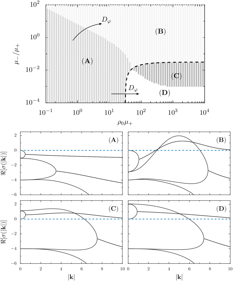
Figure 11: Results of the numerical linear stability analysis of the disordered state $p_{0}$, Eq. (10), within kinetic theory. Top: The ($\rho_{0}\mu_{+}$)-($\mu_{-}/\mu_{+}$)-plane of the parameter space. Bottom: Exemplary dispersion relations $\Re[\sigma(\left|\mathbf{k}\right|)]$ obtained numerically from (4.2). If the dispersion relation is positive, the disordered state undergoes an instability. In parameter region $(A)$, the disordered state is stable. We find Turing instabilities in the parameter range $(B)$. In $(C)$, the dispersion relation possesses a maximum at finite $\left|\vec{k}\right|$ and, additionally, the homogeneous system ($\left|\vec{k}\right|=0$) is unstable. In region $(D)$, the spatially homogeneous system is unstable. The boundary $\sigma(\left|\vec{k}\right|=0)=0$, determined by (19), is represented by a dashed line. Arrows in top panel indicate the shift of critical lines when the noise intensity $D_{\varphi}$ is increased. Parameters of dispersion relations: $\rho_{0}\mu_{+}=1$, $\mu_{-}/\mu_{+}=10^{-1}$ in (A); $\rho_{0}\mu_{+}=10^{2}$, $\mu_{-}/\mu_{+}=5\cdot 10^{-2}$ in (B); $\rho_{0}\mu_{+}=10^{2}$, $\mu_{-}/\mu_{+}=10^{-2}$ in (C); $\rho_{0}\mu_{+}=10^{2}$, $\mu_{-}/\mu_{+}=10^{-3}$ in (D); $D_{\varphi}=1.$, $\xi_{a}=0.2$, $\xi_{r}=0.1$, $\kappa_{0}\rho_{0}=1.5\cdot 10^{3}$.

The full dispersion relation cannot be obtained analytically. In order to study the linear stability of the disordered state with respect to spatially inhomogeneous perturbations, we calculated the dispersion relation numerically. Since the matrix $\tilde{M}$ is infinite dimensional, it must be truncated first. However, we can exploit that the Fourier modes ${\hat{f}}_{n}$ are damped proportional to $n^{2}$ due to angular fluctuations. Consequently, high order Fourier modes are strongly damped. Accordingly, we observe that the largest eigenvalues of the matrix (4.2) do not depend on the truncation used if a reasonably high number of Fourier modes is considered. Here, we reduce $\tilde{M}$ to a $(101\times 101)$-matrix. The results of the linear stability analysis are shown in Fig. 11.

The linear stability analysis reveals the following regimes: If the alignment-strength and the density are small, the disordered state is linearly stable (parameter region (A) in Fig. 11). An instability at finite wavelengths (Turing instability) appears if the anti-alignment strength is high (domain (B)). This instability signals the transition towards an ordered state which possesses a characteristic length scale (cf. numerical simulation in section 3). The disordered state is unstable with respect to spatially homogeneous perturbations if the alignment strength is high and anti-alignment is negligible (domain (D)). In between region (B) and (D), an intermediate regime (C) exists where the dispersion relation is positive at $\left|\vec{k}\right|=0$ but possesses a maximum at a nonzero wavenumber.

The occurrence of a Turing instability in our model is due to the concurrence of short-range alignment and anti-alignment interaction. This instability can only be found if the anti-alignment interaction is sufficiently strong. Consequently, this instability mechanism is not present in models with purely aligning interactions.

From the linear stability analysis, we cannot rigorously infer the structure of the emergent pattern which crucially depends on nonlinear terms. However, we may expect the emergence of collective states which possess a characteristic length scale in region (B) and (C). Indeed, we observe these state such as clusters of characteristic sizes, mesoscale turbulence and vortex arrays in Langevin simulations of the particle dynamics (cf. section 3, in particular Fig. 2).

4.3 Hydrodynamic theory

The linear stability analysis of the disordered state within kinetic theory revealed the existence of several instability mechanism. However, the dispersion relations could only be obtained numerically. In this section, we discuss the possibility to describe the instabilities of the disordered state analytically by a reduced set of linearized hydrodynamic equations aiming at a qualitative understanding of the macroscopic pattern formation process.

The basic assumption of the hydrodynamic theory is that only those observables in the hierarchy (4.1) are important whose large scale dynamics is slow either due to the fact that they describe a conserved quantity or they describe broken continuous symmetries. For the identification of the relevant degrees of freedom in our model, we exploit that (i) the particle number is conserved and (ii) the microscopic interaction favors local polar order due to velocity-alignment. Hence, the relevant order parameters are the particle density

$$\rho(\vec{r},t)={\hat{f}}_{0}(\vec{r},t)=\int_{0}^{2\pi}\mbox{d}\varphi\,p(\vec{r},\varphi,t)$$ (20)

and the momentum field

$$\vec{w}(\mathbf{r},t) =\int_{0}^{2\pi}\mbox{d}\varphi\,p(\vec{r},\varphi,t)\begin{pmatrix}\cos\varphi\\ \sin\varphi\end{pmatrix}=\begin{pmatrix}\Re[{\hat{f}}_{1}(\mathbf{r},t)]\\ \Im[{\hat{f}}_{1}(\mathbf{r},t)]\end{pmatrix}\!,$$ (21a)

which is proportional to the local flow field $\vec{v}(\vec{r},t)=\vec{w}(\vec{r},t)/\rho(\vec{r},t)$. Please note that we consider the order parameters locally in space. The Langevin simulations of section 3 revealed that all macroscopic patterns display local polar order. This assumption does not exclude the description of nematic states such as polar clusters moving in opposite directions (cf. Fig. 7) which possess local polar and global nematic order.

In general, the dynamics of the density and the momentum field is coupled to higher order Fourier modes. In particular, the dynamics of the polar and nematic order parameter is not independent. However, we argued above that the dynamics of the relevant order parameters is slow on large scales. The assumption of fast relaxation of higher order Fourier modes enables us to truncate the hierarchy (4.1) at low order. In particular, we express the nematic order parameter as a function of the polar order parameter and the density by adiabatic elimination, and further neglect all higher order Fourier coefficients following the same reasoning. Here, we focus on linear terms since we are interested in comparing the predictions of the linear stability analysis of the disordered state. We obtain the following set of linearized hydrodynamic equations:

$$\frac{\partial\rho}{\partial t}= -\nabla\cdot\mathbf{w},$$ (22a)

$$\frac{\partial\mathbf{w}}{\partial t}\approx -\left(\frac{1}{2}+\frac{\pi\rho_{0}\kappa_{0}\xi_{r}^{3}}{6}\right)\!\nabla\rho-D_{\varphi}\mathbf{w}+\pi\rho_{0}\hat{\mu}_{\Delta}\mathbf{w}+\frac{\Delta\mathbf{w}}{16D_{\varphi}}\,.$$ (22b)

The continuity equation (22a) reflects the conservation of the number of particles. The equation for the momentum field contains several physical effects. The first term which is proportional to the gradient of the density describes a macroscopic particle flow compensating density gradients. The prefactor in brackets is proportional to the pressure which contains two contributions: (i) the constant term is due to the active motion; (ii) the second term is proportional to the repulsive force which effectively increases the pressure, i.e. it reduces the compressibility. The second term in (22b) accounts for the effect of noise counteracting the emergence of polar order. The nonlocal alignment interaction is described by the operator $\hat{\mu}_{\Delta}$ defined via a series of Laplacian operators (13). The last term represents the reduction of the effective viscosity due to angular noise. It is the only term which is influenced by the truncation scheme used to derive (22).

Linear stability analysis within the hydrodynamic theory

The truncation of the infinite hierarchy of Fourier modes to the simplified system of hydrodynamic equations is a considerable simplification. In particular, it allows the analytical calculation of the dispersion relations which can be directly obtained by Fourier transformation of the hydrodynamic equations (22) and subsequent matrix diagonalization:

$$\sigma_{1}\!\left(\left|\mathbf{k}\right|\right) =\pi\rho_{0}\hat{\mu}_{k}-D_{\varphi}-\frac{\left|\mathbf{k}\right|^{2}}{16D_{\varphi}},$$ (23a)

$$\sigma_{2,3}\!\left(\left|\mathbf{k}\right|\right) =\frac{1}{2}\left[\sigma_{1}\!\left(\left|\mathbf{k}\right|\right)\pm\sqrt{\left[\sigma_{1}\!\left(\left|\mathbf{k}\right|\right)\right]^{2}-2\left(1+\frac{\pi\rho_{0}\kappa_{0}\xi_{r}^{3}}{3}\right)\!\left|\mathbf{k}\right|^{2}}\,\,\right]\!.$$ (23b)

We address the question in which parameter range this approximation is applicable and whether these approximated dispersion relations can be used to describe the destabilization of the disordered state.

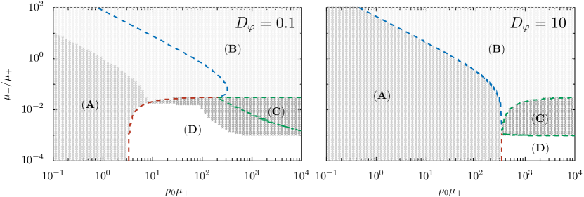
Figure 12: Comparison of the results of the linear stability analysis of the spatially homogeneous state using the Fokker-Planck equation (8) and the hydrodynamic approximation (22). The results corresponding to the kinetic theory are shown in the same way as in Fig. 11. Predictions of the hydrodynamic theory are shown by lines. In the high noise limit (right), the hydrodynamic approximation is exact, whereas deviations are found for low noise values (left). Parameters: $D_{\varphi}=0.1$ (left), $D_{\varphi}=10$ (right). Other parameters: see Fig. 11.

The results of the parameter study are illustrated in Fig. 12. The analysis was performed for high and low noise values $D_{\varphi}$. For high noise amplitudes, we obtain perfect agreement of the predictions of the hydrodynamic equations (22) with the results of the linear stability analysis which was based on the one-particle Fokker-Planck equation (8). However, the predictions of the hydrodynamic theory deviate from the kinetic theory in the limit of low noise values. These deviations are due to the adiabatic elimination of the second Fourier mode and the negligence of all higher Fourier coefficients. These deviations could have been expected: The assumption that high order Fourier modes relax fast is only justifiable for high noise values, since $D_{\varphi}$ determines the relaxation rate of the Fourier coefficients as can be seen from (4.1).

Consequently, we conclude that it is possible to describe the linear dynamics of the system by the hydrodynamic equations (22) as long as the noise strength is high, i.e. a considerable timescale separation between the lowest and higher Fourier coefficients exists.

Approximating the nonlocal alignment interaction

As already mentioned in section 4.1, one can possibly approximate the infinite series $\hat{\mu}_{\Delta}$ of Laplacian operators by a truncated polynomial:

$$\hat{\mu}_{\Delta}\approx\hat{\mu}_{\Delta,N_{c}}=\sum_{n=0}^{N_{c}}\left[\int_{0}^{\infty}\mbox{d}r\,r\mu(r)\,\frac{r^{2n}}{4^{n}(n!)^{2}}\right]\!\Delta^{n}.$$ (24)

Naturally, this raises the question how to choose $N_{c}$ (order of truncation) and how reliable the corresponding approximations are. The stability of the dynamics requires that

$$(-1)^{N_{c}}\left[\int_{0}^{\infty}\mbox{d}r\,\mu(r)\,r^{2N_{c}+1}\right]<0$$ (25)

holds. As a rule of thumb, (25) reflects that $N_{c}$ must be odd if alignment interaction dominates and $N_{c}$ must be even if anti-alignment is predominant.

What is the nature of an approximation like (24)? The operator $\hat{\mu}_{\Delta}$ describing the nonlocal (anti-)alignment interaction is linear and, thus, it possesses a characteristic spectrum $\hat{\mu}_{k}$ introduced in Eq. (18). Approximating the operator by a series of Laplacian operators, cf. (24), is equivalent to approximate the spectrum by a Taylor series in powers of the wavenumber $\left|\vec{k}\right|$ around $\left|\vec{k}\right|=0$ restricting the applicability of this approximation to small wavenumbers (large length scales). The stability requirement (25) ensures that the spectrum at large wavenumbers is negative. Otherwise, fluctuations on small length-scales would be amplified without any bound.

On phenomenological grounds, there are two conceivable types of spectra:

1. the spectrum possesses a maximum at $\left|\vec{k}\right|=0$ and decreases monotonically;

2. the spectrum possesses a maximum at a finite wavenumber.

The former case was studied in the context of the Vicsek model (pure alignment interaction vicsek_novel_1995 ) in the corresponding field theory by Toner and Tu toner_LRO_1995 . The latter was recently proposed by Dunkel et al. dunkel_minimal_2013 in order to describe mesoscale turbulence. Using the expansion of the operator $\hat{\mu}_{\Delta}$, we can map our linearized hydrodynamic theory to these phenomenological equations

$$\frac{\partial\rho}{\partial t}= -\nabla\cdot\mathbf{w},$$ (26a)

$$\frac{\partial\mathbf{w}}{\partial t}\approx -\left(\frac{1}{2}+\frac{\pi\rho_{0}\kappa_{0}\xi_{r}^{3}}{6}\right)\!\nabla\rho+\alpha\hskip 0.85355pt\mathbf{w}+\Gamma_{0}\Delta\mathbf{w}+\Gamma_{2}\Delta^{2}\mathbf{w},$$ (26b)

and derive the dependency of transport coefficients on microscopic model parameters

$$\alpha =\pi\rho_{0}\left(\int_{0}^{\infty}\mbox{d}r\,r\mu(r)\right)-D_{\varphi},$$ (27a)

$$\Gamma_{0} =\frac{\pi\rho_{0}}{4}\left(\int_{0}^{\infty}\mbox{d}r\,r^{3}\mu(r)\right)+\frac{1}{16D_{\varphi}}\,,$$ (27b)

$$\Gamma_{2} =\frac{\pi\rho_{0}}{64}\int_{0}^{\infty}\mbox{d}r\,r^{5}\mu(r).$$ (27c)

The linearized hydrodynamic equations can describe a Turing instability of the disordered state if the effective viscosity $\Gamma_{0}$ is negative dunkel_minimal_2013 , i.e. only if the anti-alignment interaction is sufficiently strong.

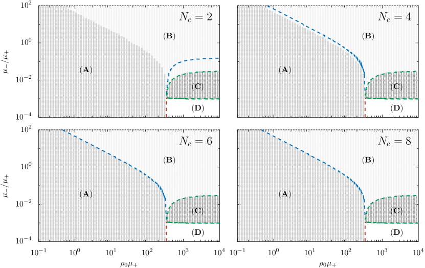
Figure 13: Domains of stability and instability of the disordered state. Predictions of the kinetic theory (8) are depicted as gray shaded regions (cf. Fig. 11). The colored lines are derived from the dispersion relations of the linearized hydrodynamic theory (22) for different values of the truncation parameter $N_{c}$, cf. Eq. (24). The critical line of the Turing instability (blue dashed line separating (A) and (B)) is not correctly predicted in the case $N_{c}=2$. Qualitative agreement is achieved for $N_{c}=4$, higher order approximations are almost exact. Parameters: $D_{\varphi}=10$, others as in Fig. 11.

It is a priori not clear how many terms are necessary in order to reproduce quantitatively the instabilities found from kinetic theory using a truncated operator $\hat{\mu}_{\Delta,N_{c}}$. We close this paragraph by answering this question for our model. In the case of $N_{c}=0$, the results deduced from the spatially homogeneous equations are recovered (cf. Eq. (19)). The results of the linear stability analysis for $N_{c}\in\left\{2,4,6,8\right\}$ are shown in Fig. 13. It is evident from our analysis that it is insufficient to approximate $\hat{\mu}_{\Delta}$ in the leading order $N_{c}=2$. The disagreement is due to the fact that not all relevant length scales are resolved properly in this case. However, the situation is essentially different if the approximation $N_{c}=4$ is used. This approximation enables the qualitative prediction of the structure of the phase space. Higher order approximations $N_{c}\geq 6$ can be considered as almost exact on the linear level. We stress that the number of terms which are necessary to reproduce the spectrum $\hat{\mu}_{k}$ sufficiently well, i.e. how many terms are necessary to resolve all relevant length scales, is not a universal number but depends on model details.

4.4 Conclusions

The analysis presented in this chapter reveals the existence of a Turing instability of the coarse-grained velocity field due to the anti-alignment interaction – there exists a region in parameter space where the dynamics of the system is linearly unstable at finite wavelengths. Furthermore, we showed that a system of hydrodynamic equations (26), where the nonlocal operator $\hat{\mu}_{\Delta}$ is approximated by a truncated series, provides an excellent approximation for the prediction of phase boundaries given the following conditions are fulfilled:

• The dynamics of the Fourier coefficients decouple, i.e. the truncation of the hierarchy of Fourier modes is possible, if a considerable timescale separation among the modes exists. In particular, high Fourier modes are strongly damped if angular fluctuations are large justifying the negligence of these high order modes. This property allows to truncate the infinite hierarchy of Fourier modes and enables us to replace it by a low dimensional system.

• The nonlocal interaction operator must be approximated sufficiently well, i.e. the series expansion of $\hat{\mu}_{\Delta}$ must contain enough terms in order to resolve all relevant length scales. In our particular model, this is the case if all terms including the term proportional to $\Delta^{6}\,\vec{w}$ are taken into account.

The linearized theory discussed here is not capable of predicting the macroscopic patterns since nonlinear terms were not considered for simplicity. However, the theory confirms the existence of a Turing instability of the polar order parameter in our model. Such an instability mechanism was proposed in dunkel_minimal_2013 on phenomenological grounds and shown to be sufficient to explain mesoscale turbulence in dense bacterial suspensions wensink_meso-scale_2012 ; dunkel_fluid_2013 . In this work, we provide a microscopic explanation of this instability: the concurrence of short-range creation of local polar order with an opposing effect on larger scales.

5 Summary

We studied the pattern formation in an ensemble of self-propelled particles which move at constant speed and interact via competing velocity-alignment interactions: at short length scales, particles tend to align their velocities whereas they anti-align their direction of motion with particles which are further away grossmann_vortex_2014 . The interplay of alignment and anti-alignment interaction has to be understood as an effective description of two competing mechanisms: locally, polar order arises due to anisotropic steric interactions or inelastic collisions for example, whereas the emergence of global polar order is suppressed by an opposing effect, e.g. hydrodynamic interaction.

Numerical simulations of the particle dynamics reveal the emergence of surprisingly complex spatio-temporal pattern formation. On the one hand, our model reduces to a continuous time version of the Vicsek model vicsek_novel_1995 ; peruani_mean_2008 for vanishing anti-alignment interaction. Therefore, we observe a phenomenology similar to the Vicsek model chate_collective_2008 in this limiting case. Especially, large scale traveling bands emerge in the low density regime close to the onset of polar order. Moreover, numerous additional phases were found due to the anti-alignment interaction. If this interaction is strong and the particle density is high, we observe vortex arrays and synchronously rotating cluster. By gradually lowering the anti-alignment interaction, the velocity-alignment acting on short length scales induces local polar order and, thus, mesoscopic convective flows. In this intermediate regime, the anti-alignment interaction inhibits the emergence of global polar order and, consequently, we observe a rotationally invariant state possessing local polar order but global disorder (mesoscale turbulence). Another characteristic of this state is the emergence of transient vortices, which are separated by a characteristic length. Moreover, we observe extended convective flows (jets). At low densities, the actual patterns differ strongly: We observe small polar clusters moving randomly for intermediate anti-alignment strength. At strong anti-alignment, the system exhibits large scale nematic order as polar clusters start to form lanes moving in opposite directions.

Common to all the patterns is a characteristic length scale which manifests itself mainly in the momentum field. Studying the linear stability of the disordered state within mean-field theory, we were able to relate this pattern formation process to a Turing instability. Furthermore, we analyzed in detail the possibility of describing this instability using a reduced set of hydrodynamic equations. We showed that a system of hydrodynamic equations can quantitatively reproduce the relevant instabilities if two conditions are fulfilled: (i) the reduction to a low dimensional system of order parameter equations is only possible if a considerable timescale separation between fast and slow modes exists which is particularly fulfilled for high noise in our model; (ii) the nonlocal interaction has to be described sufficiently well by taking into account a high number of derivatives in the coarse-grained description.

Based on the analysis of our self-propelled particle model, we suggest that the interplay of competing alignment interactions may generally give rise to a Turing instability in the polar order parameter field and that this mechanism in combination with convective particle transport can explain the emergence of mesoscale turbulence and vortex arrays in active matter systems.

Appendix A Mean-field approximation

The derivation of the nonlinear Fokker-Planck equation (8) relies on a mean-field approximation (MFA) – the negligence of fluctuations – which we illustrate in detail in this section. The central quantity is the microscopic particle density $\mathcal{P}(\vec{r},\varphi,t)$ defined by

$$\mathcal{P}(\vec{r},\varphi,t)=\sum_{i=1}^{N}\delta^{(2)}(\vec{r}-\vec{r}_{i}(t))\delta(\varphi-\varphi_{i}(t))$$ (28)

which is a stochastic fluctuating field variable. From this field, we can compute the one-particle probability density function to find a particle at position $\vec{r}$ with orientation $\varphi$ at time $t$ via

$$P_{1}(\vec{r},\varphi,t)=\frac{\left<\sum_{i=1}^{N}\delta^{(2)}(\vec{r}-\vec{r}_{i}(t))\delta(\varphi-\varphi_{i}(t))\right>}{N}=\frac{\left<\mathcal{P}(\vec{r},\varphi,t)\right>}{N}$$ (29)

as well as the two-particle probability density function to find one particle at position $\vec{r}$ with orientation $\varphi$ and another particle at position $\vec{r}^{\prime}$ with orientation $\varphi^{\prime}$ at time $t$ via

$$P_{2}(\vec{r},\varphi;\vec{r}^{\prime},\varphi^{\prime};t) =\frac{\left<\sum_{i,j;i\neq j}\delta^{(2)}(\vec{r}-\vec{r}_{i}(t))\delta^{(2)}(\vec{r}^{\prime}-\vec{r}_{j}(t))\delta(\varphi-\varphi_{i}(t))\delta(\varphi^{\prime}-\varphi_{j}(t))\right>}{N(N-1)}$$ (30a)

$$=\frac{\left<\mathcal{P}(\vec{r},\varphi,t)\mathcal{P}(\vec{r}^{\prime},\varphi^{\prime},t)\right>}{N(N-1)}-\frac{P_{1}(\vec{r},\varphi,t)\delta^{(2)}(\vec{r}-\vec{r}^{\prime})\delta(\varphi-\varphi^{\prime})}{N-1}.$$ (30b)

In mean-field approximation, fluctuating variables are approximated by their average values thus neglecting fluctuations:

$$\mathcal{P}(\vec{r},\varphi,t) =\left<\mathcal{P}(\vec{r},\varphi,t)\right>+\delta\mathcal{P}(\vec{r},\varphi,t)\,{\underset{\text{(MFA)}}{\approx}}\,\left<\mathcal{P}(\vec{r},\varphi,t)\right>.$$ (31)

Therefore, we deduce from (30b) that we can approximate the two-particle probability density function by the product of one-particle probability densities:

$$P_{2}(\vec{r},\varphi;\vec{r}^{\prime},\varphi^{\prime};t) {\underset{\text{(MFA)}}{\approx}}\frac{NP_{1}(\vec{r},\varphi,t)P_{1}(\vec{r}^{\prime},\varphi^{\prime},t)}{N-1}-\frac{P_{1}(\vec{r},\varphi,t)\delta^{(2)}(\vec{r}-\vec{r}^{\prime})\delta(\varphi-\varphi^{\prime})}{N-1}$$ (32a)

$${\underset{(N\rightarrow\infty)}{\approx}}\,P_{1}(\vec{r},\varphi,t)P_{1}(\vec{r}^{\prime},\varphi^{\prime},t).$$ (32b)

Thus, the mean-field approximation is equivalent to the negligence of inter-particle correlations.

References

- (1) J. Toner, Y. Tu, S. Ramaswamy, Annals of Physics 318, 170 (2005)
- (2) P. Romanczuk, M. Bär, W. Ebeling, B. Lindner, L. Schimansky-Geier, The European Physical Journal - Special Topics 202, 1 (2012)
- (3) T. Vicsek, A. Zafeiris, Physics Reports 517, 71 (2012)
- (4) M.C. Marchetti, J.F. Joanny, S. Ramaswamy, T.B. Liverpool, J. Prost, M. Rao, R.A. Simha, Reviews of Modern Physics 85, 1143 (2013)
- (5) A.M. Menzel, Physics Reports 554, 1 (2015)
- (6) V. Schaller, C. Weber, C. Semmrich, E. Frey, A.R. Bausch, Nature 467, 73 (2010)
- (7) I. Theurkauff, C. Cottin-Bizonne, J. Palacci, C. Ybert, L. Bocquet, Physical Review Letters 108, 268303 (2012)
- (8) O. Pohl, H. Stark, Physical Review Letters 112, 238303 (2014)
- (9) A. Czirók, E. Ben-Jacob, I. Cohen, T. Vicsek, Physical Review E 54, 1791 (1996)
- (10) A. Sokolov, I.S. Aranson, J.O. Kessler, R.E. Goldstein, Physical Review Letters 98, 158102 (2007)
- (11) F. Peruani, J. Starruß, V. Jakovljevic, L. Søgaard-Andersen, A. Deutsch, M. Bär, Physical Review Letters 108, 098102 (2012)
- (12) C. Dombrowski, L. Cisnero, S. Chatkaew, R.E. Goldstein, J.O. Kessler, Physical Review Letters 93, 098103 (2004)
- (13) A. Sokolov, R.E. Goldstein, F.I. Feldchtein, I.S. Aranson, Physical Review E 80, 031903 (2009)
- (14) L.H. Cisneros, R. Cortez, C. Dombrowski, R.E. Goldstein, J.O. Kessler, in Animal Locomotion, edited by G.K. Taylor, M.S. Triantafyllou, C. Tropea (Springer Berlin Heidelberg, 2010), pp. 99–115
- (15) H.H. Wensink, J. Dunkel, S. Heidenreich, K. Drescher, R.E. Goldstein, H. Löwen, J.M. Yeomans, Proceedings of the National Academy of Sciences 109, 14308 (2012)
- (16) H.P. Zhang, A. Be’er, R.S. Smith, E.L. Florin, H.L. Swinney, Europhysics Letters 87, 48011 (2009)
- (17) K.A. Liu, L. I, Physical Review E 86, 011924 (2012)
- (18) M. Ballerini, N. Cabibbo, R. Candelier, A. Cavagna, E. Cisbani, I. Giardina, V. Lecomte, A. Orlandi, G. Parisi, A. Procaccini et al., Proceedings of the National Academy of Sciences 105, 1232 (2008)
- (19) Y. Katz, K. Tunstrøm, C.C. Ioannou, C. Huepe, I.D. Couzin, Proceedings of the National Academy of Sciences 108, 18720 (2011)
- (20) Y. Sumino, K.H. Nagai, Y. Shitaka, D. Tanaka, K. Yoshikawa, H. Chaté, K. Oiwa, Nature 483, 448 (2012)
- (21) J. Dunkel, S. Heidenreich, K. Drescher, H.H. Wensink, M. Bär, R.E. Goldstein, Physical Review Letters 110, 228102 (2013)
- (22) J. Toner, Physical Review E 86, 031918 (2012)
- (23) L. Chen, J. Toner, C.F. Lee, arXiv:1410.2764 (2014)
- (24) J. Swift, P.C. Hohenberg, Physical Review A 15, 319 (1977)
- (25) R. Großmann, P. Romanczuk, M. Bär, L. Schimansky-Geier, Physical Review Letters 113, 258104 (2014)
- (26) A.M. Turing, Philosophical Transactions of the Royal Society of London. Series B, Biological Sciences 237, 37 (1952)
- (27) S. Krinsky, D. Mukamel, Physical Review B 16, 2313 (1977)
- (28) M.N. Barber, Journal of Physics A: Mathematical and General 12, 679 (1979)
- (29) J. Oitmaa, Journal of Physics A: Mathematical and General 14, 1159 (1981)
- (30) H. Hong, S.H. Strogatz, Physical Review Letters 106, 054102 (2011)
- (31) T. Vicsek, A. Czirók, E. Ben-Jacob, I. Cohen, O. Shochet, Physical Review Letters 75, 1226 (1995)
- (32) H. Chaté, F. Ginelli, G. Grégoire, F. Peruani, F. Raynaud, European Physical Journal B 64, 451 (2008)
- (33) A.M. Menzel, Physical Review E 85, 021912 (2012)
- (34) V. Lobaskin, M. Romenskyy, Physical Review E 87, 052135 (2013)
- (35) A. Mikhailov, D. Meinköhn, in Stochastic Dynamics, edited by L. Schimansky-Geier, T. Pöschel (Springer Berlin Heidelberg, 1997), Vol. 484 of Lecture Notes in Physics, pp. 334–345
- (36) C. Weber, P.K. Radtke, L. Schimansky-Geier, P. Hänggi, Physical Review E 84, 011132 (2011)
- (37) C. Weber, I.M. Sokolov, L. Schimansky-Geier, Physical Review E 85, 052101 (2012)
- (38) A. Baskaran, M.C. Marchetti, Proceedings of the National Academy of Sciences 106, 15567 (2009)
- (39) H. Chaté, F. Ginelli, G. Grégoire, F. Raynaud, Physical Review E 77, 046113 (2008)
- (40) E. Bertin, M. Droz, G. Grégoire, Journal of Physics A: Mathematical and Theoretical 42, 445001 (2009)
- (41) A.M. Menzel, H. Löwen, Physical Review Letters 110, 055702 (2013)
- (42) A.M. Menzel, T. Ohta, H. Löwen, Physical Review E 89, 022301 (2014)
- (43) D. Helbing, I.J. Farkas, T. Vicsek, Physical Review Letters 84, 1240 (2000)
- (44) H.H. Wensink, H. Löwen, Journal of Physics: Condensed Matter 24, 464130 (2012)
- (45) S.R. McCandlish, A. Baskaran, M.F. Hagan, Soft Matter 8, 2527 (2012)
- (46) F. Peruani, A. Deutsch, M. Bär, The European Physical Journal - Special Topics 157, 111 (2008)
- (47) F.D.C. Farrell, M.C. Marchetti, D. Marenduzzo, J. Tailleur, Physical Review Letters 108, 248101 (2012)
- (48) R. Großmann, L. Schimansky-Geier, P. Romanczuk, New Journal of Physics 15, 085014 (2013)
- (49) J. Toner, Y. Tu, Physical Review Letters 75, 4326 (1995)
- (50) J. Dunkel, S. Heidenreich, M. Bär, R.E. Goldstein, New Journal of Physics 15, 045016 (2013)