Accurate and efficient numerical methods for computing ground states and dynamics of dipolar Bose-Einstein condensates via the nonuniform FFT

Abstract

In this paper, we propose efficient and accurate numerical methods for computing the ground state and dynamics of the dipolar Bose-Einstein condensates utilising a newly developed dipole-dipole interaction (DDI) solver that is implemented with the non-uniform fast Fourier transform (NUFFT) algorithm. We begin with the three-dimensional (3D) Gross-Pitaevskii equation (GPE) with a DDI term and present the corresponding two-dimensional (2D) model under a strongly anisotropic confining potential. Different from existing methods, the NUFFT based DDI solver removes the singularity by adopting the spherical/polar coordinates in Fourier space in 3D/2D, respectively, thus it can achieve spectral accuracy in space and simultaneously maintain high efficiency by making full use of FFT and NUFFT whenever it is necessary and/or needed. Then, we incorporate this solver into existing successful methods for computing the ground state and dynamics of GPE with a DDI for dipolar BEC. Extensive numerical comparisons with existing methods are carried out for computing the DDI, ground states and dynamics of the dipolar BEC. Numerical results show that our new methods outperform existing methods in terms of both accuracy and efficiency.

Dedicated to Professor Eitan Tadmor on the occasion of his 60th birthday

1 Introduction

Since its first experimental creation in 1995 [4, 20, 23], the Bose-Einstein condensation (BEC) has provided an incredible glimpse into the macroscopic quantum world and opened a new era in atomic and molecular physics as well as condensated matter physics. It regains vast interests and has been extensively studied both experimentally and theoretically [3, 17, 19, 24, 34, 37, 41]. At early stage, experiments mainly realize BECs of ultracold atomic gases whose properties are mainly governed by the isotropic and short-range interatomic interactions [41]. However, recent experimental developments on Feshbach resonances [31], on cooling and trapping molecules [38, 44] and on precision measurements and control [47, 42] allow one to realize BECs of quantum gases with different, richer interactions and gain even more interesting properties. In particular, the successful realization of BECs of dipolar quantum gases with long-range and anisotropic dipolar interaction, e.g., ${}^{52}{\rm Cr}$ [26], ${}^{164}{\rm Dy}$ [35] and ${}^{168}{\rm Er}$ [2], has spurred great interests in the unique properties of degenerate dipolar quantum gases and stimulated enthusiasm in studying both the ground state [8, 7, 29, 43, 48] and dynamics [14, 13, 22, 27, 33, 40] of dipolar BECs.

At temperatures $T$ much smaller than the critical temperature $T_{c}$, the properties of BEC with long-range dipole-dipole interactions (DDI) are well described by the macroscopic complex-valued wave function $\psi=\psi(\mathbf{x},t)$ whose evolution is governed by the celebrating three-dimensional (3D) Gross–Pitaevskii equation (GPE) with a DDI term. Moreover, the 3D GPE can be reduced to an effective two-dimensional (2D) version if the external trapping potential is strongly confined in the $z-$direction [21, 8]. In a unified way, the dimensionless GPE with a DDI term in $d-$dimensions ($d=2\ {\rm or}\ 3$) for modeling a dipolar BEC reads as [14, 6, 7, 25, 48]:

$$i\partial_{t}\psi({\mathbf{x}},t)=\left[-\frac{1}{2}\nabla^{2}+V({\bf x})+\beta|\psi|^{2}+\lambda\,\Phi(\mathbf{x},t)\right]\psi(\mathbf{x},t),\quad\mathbf{x}\in{\mathbb{R}}^{d},\quad t>0,$$ (1.1)

$$\Phi(\mathbf{x},t)=\left(U_{\rm dip}\ast|\psi|^{2}\right)(\mathbf{x},t),\qquad\qquad\mathbf{x}\in{\mathbb{R}}^{d},\quad t\geq 0,$$ (1.2)

$$\psi(\mathbf{x},t=0)=\psi_{0}(\mathbf{x}),\qquad\qquad\;\mathbf{x}\in{\mathbb{R}}^{d},$$ (1.3)

where $t$ is time, ${\bf x}=(x,y)^{T}\in{\mathbb{R}}^{2}$ or ${\bf x}=(x,y,z)^{T}\in{\mathbb{R}}^{3}$, $\ast$ represents the convolution operator with respect to spatial variable. The dimensionless constant $\beta$ describes the strength of the short-range two-body interactions in a condensate (positive for repulsive interaction, and resp. negative for attractive interaction), while $V(\mathbf{x})$ is a given real-valued external trapping potential which is determined by the type of system under investigation. In most BEC experiments, a harmonic potential is chosen to trap the condensate, i.e.,

$$V(\mathbf{x})=\frac{1}{2}\left\{\begin{array}[]{ll}\gamma_{x}^{2}x^{2}+\gamma_{y}^{2}y^{2},&d=2,\\[3.00003pt] \gamma_{x}^{2}x^{2}+\gamma_{y}^{2}y^{2}+\gamma_{z}^{2}z^{2},&d=3,\end{array}\right.$$ (1.4)

where $\gamma_{x}>0$, $\gamma_{y}>0$ and $\gamma_{z}>0$ are dimensionless constants proportional to the trapping frequencies in $x$-, $y$- and $z$-direction, respectively. Moreover, $\lambda$ is a dimensionless constant characterizing the strength of DDI and $\Phi(\mathbf{x},t)$ is the long-range dipole interaction whose convolution kernel in 3D/2D is given as [6, 14, 21, 8, 28]:

$$U_{\rm dip}(\mathbf{x})=\left\{\begin{array}[]{l}-\delta(\mathbf{x})-3\,\partial_{\mathbf{n}\mathbf{n}}\left(\frac{1}{4\pi|\mathbf{x}|}\right),\\[5.0pt] -\frac{3}{2}\left(\partial_{\mathbf{n}_{\perp}\mathbf{n}_{\perp}}-n_{3}^{2}\nabla_{\perp}^{2}\right)\left(\frac{1}{2\pi|\mathbf{x}|}\right),\end{array}\right.\Leftrightarrow\;\;\widehat{U}_{\rm dip}(\mathbf{k})=\left\{\begin{array}[]{ll}-1+\frac{3(\mathbf{n}\cdot\mathbf{k})^{2}}{\|\mathbf{k}\|^{2}},&d=3,\\[5.0pt] \frac{3\left[(\mathbf{n}_{\perp}\cdot\mathbf{k})^{2}-n_{3}^{2}\|\mathbf{k}\|^{2}\right]}{2\|\mathbf{k}\|},&d=2,\end{array}\right.$$ (1.5)

where $\mathbf{x},\mathbf{k}\in\mathbb{R}^{d}$ and $\widehat{f}(\mathbf{k})=\int_{{\mathbb{R}}^{d}}f(\mathbf{x})\;e^{-i\mathbf{k}\cdot\mathbf{x}}\,d\mathbf{x}$ is the Fourier transform of $f(\mathbf{x})$. Here, $\mathbf{n}=(n_{1},n_{2},n_{3})^{T}$ is a given unit vector representing the dipole axis, $\mathbf{n}_{\perp}=(n_{1},n_{2})^{T}$, $\partial_{\mathbf{n}}=\mathbf{n}\cdot\nabla$, $\partial_{\mathbf{n}\mathbf{n}}=\partial_{\mathbf{n}}(\partial_{\mathbf{n}})$, $\nabla_{\perp}=(\partial_{x},\partial_{y})^{T}$, $\partial_{\mathbf{n}_{\perp}}=\mathbf{n}_{\perp}\cdot\nabla_{\perp}$ and $\partial_{\mathbf{n}_{\perp}\mathbf{n}_{\perp}}=\partial_{\mathbf{n}_{\perp}}(\partial_{\mathbf{n}_{\perp}}).$ Note that the dipole axis can also be different. The dipole kernel $U_{\rm dip}(\mathbf{x})$ with two different dipole orientations $\mathbf{n}$ and $\mathbf{m}$ reads as [28, 39, 6]

$$U_{\rm dip}(\mathbf{x})=\left\{\begin{array}[]{ll}-(\mathbf{n}\cdot\mathbf{m})\delta(\mathbf{x})-3\,\partial_{\mathbf{n}\mathbf{m}}\left(\frac{1}{4\pi|\mathbf{x}|}\right),&\mathbf{x}\in{\mathbb{R}}^{3},\\ -\frac{3}{2}\left(\partial_{\mathbf{n}_{\perp}\mathbf{m}_{\perp}}-n_{3}m_{3}\nabla_{\perp}^{2}\right)\left(\frac{1}{2\pi|\mathbf{x}|}\right),&\mathbf{x}\in{\mathbb{R}}^{2},\end{array}\right.$$ (1.6)

where $\mathbf{m}=(m_{1},m_{2},m_{3})^{T}$ is a given unit vector representing the other dipole orientation, $\mathbf{m}_{\perp}=(m_{1},m_{2})^{T}$, $\partial_{\mathbf{m}_{\perp}}=\mathbf{m}_{\perp}\cdot\nabla_{\perp}$ and $\partial_{\mathbf{n}_{\perp}\mathbf{m}_{\perp}}=\partial_{\mathbf{n}_{\perp}}(\partial_{\mathbf{m}_{\perp}})$. We remark here that in most physical experiments, the dipoles are polarized at the same direction, i.e., $\mathbf{m}=\mathbf{n}$, thus, hereafter, we always assume $\mathbf{m}=\mathbf{n}$ unless specified otherwise.

The GPE (1.1)-(1.3) conserves two important quantities: the mass (or normalization) of the wave function

$$N(t):=\|\psi(\cdot,t)\|^{2}:=\int_{{\mathbb{R}}^{d}}|\psi({\mathbf{x}},t)|^{2}d{\bf x}\equiv\int_{{\mathbb{R}}^{d}}|\psi({\bf x},0)|^{2}d{\bf x}=1,\qquad t\geq 0,$$ (1.7)

and the energy per particle

$$E(\psi(\cdot,t))=\int_{{\mathbb{R}}^{d}}\left[\frac{1}{2}|\nabla\psi|^{2}+V({\bf x})|\psi|^{2}+\frac{\beta}{2}|\psi|^{4}+\frac{\lambda}{2}\Phi(\mathbf{x},t)\,|\psi|^{2}\right]d{\bf x}\equiv E(\psi(\cdot,0)),\qquad t\geq 0.$$ (1.8)

The ground state $\phi_{g}$ of the GPE (1.1)-(1.3) is defined as follows:

$$\phi_{g}=\arg\min_{\phi\in S}E(\phi),\quad\hbox{where}\quad S:=\{\phi(\mathbf{x})\ |\ \|\phi\|^{2}:=\int_{{\mathbb{R}}^{d}}|\phi(\mathbf{x})|^{2}d\mathbf{x}=1,\ E(\phi)<\infty\}.$$ (1.9)

Extensive works have been carried out to study the ground state and dynamics of dipolar BEC based on the GPE (1.1)-(1.3). For existing theoretical and numerical studies, we refer to [22, 7, 17, 32, 21, 30, 33] and [12, 13, 18, 27, 25, 33, 46, 5], respectively, and references therein.

To compute the ground state and dynamics of the GPE (1.1), one of the key difficulties is how to evaluate the nonlocal dipole interaction $\Phi(\mathbf{x},t)$ (1.2) accurately and effectively for a given density $\rho=|\psi|^{2}$. Noticing that

$$\Phi(\mathbf{x},t)=\int_{{\mathbb{R}}^{d}}U_{\rm dip}(\mathbf{x}-\mathbf{y})\rho(\mathbf{y},t)d\mathbf{y}=\frac{1}{(2\pi)^{d}}\int_{{\mathbb{R}}^{d}}\widehat{U}_{\rm dip}(\mathbf{k})\,\widehat{\rho}(\mathbf{k},t)\,e^{i\,\mathbf{k}\cdot\mathbf{x}}\,d\mathbf{k},$$ (1.10)

it is natural to evaluate $\Phi(\mathbf{x},t)$ via the standard fast Fourier transform (FFT) using a uniform grid on a bounded computational domain [18, 39, 40, 46]. Nevertheless, due to the intrinsic singularity/discontinuity of $\widehat{U}_{\rm dip}(\mathbf{k})$ at the origin $\mathbf{k}={\bf 0}$, the so called “numerical locking” phenomena occurs, which limits the optimal accuracy on any given computational domain [7, 49]. To alleviate this problem, another approach [8, 21] is to reformulate the convolution (1.2) with 3D dipole kernel (1.5) in terms of the Poisson equation:

$$-\Delta\;u(\mathbf{x},t)=|\psi(\mathbf{x},t)|^{2},\qquad\lim_{|\mathbf{x}|\rightarrow\infty}u(\mathbf{x},t)=0,\qquad\mathbf{x}\in{\mathbb{R}}^{3},\quad t\geq 0,$$ (1.11)

and convolution (1.2) with 2D dipole kernel (1.5) in terms of the fractional Position equation

$$\sqrt{-\Delta}\;u(\mathbf{x},t)=|\psi(\mathbf{x},t)|^{2},\qquad\lim_{|\mathbf{x}|\rightarrow\infty}u(\mathbf{x},t)=0,\qquad\mathbf{x}\in{\mathbb{R}}^{2},\quad t\geq 0.$$ (1.12)

Then, the dipolar potential $\Phi(\mathbf{x},t)$ can be computed by a differentiation of $u(\mathbf{x},t)$ as:

$$\Phi(\mathbf{x},t)=\left\{\begin{array}[]{ll}-|\psi(\mathbf{x},t)|^{2}-3\partial_{\mathbf{n}\mathbf{n}}u(\mathbf{x},t),&\mathbf{x}\in{\mathbb{R}}^{3},\\[8.00003pt] -\frac{3}{2}\left(\partial_{\mathbf{n}_{\perp}\mathbf{n}_{\perp}}-n_{3}^{2}\nabla_{\perp}^{2}\right)u(\mathbf{x},t),&\mathbf{x}\in{\mathbb{R}}^{2},\end{array}\right.\qquad t\geq 0.$$ (1.13)

Then in practical computations, the sine pseudospectral method is applied to solve (1.11)-(1.13) on a truncated rectangular domain $\Omega$ with homogeneous Dirichlet boundary conditions imposed on $\partial\Omega$, and they can be implemented with discrete sine transform (DST) efficiently and accurately [8]. By waiving the use of the ${\bf 0}$-mode in the Fourier space, the sine spectral method significantly improves the accuracy for the dipole interaction evaluation. However, due to the polynomial decaying property of $u(\mathbf{x},t)$ when $|\mathbf{x}|\to\infty$, a very large computational domain is required in order to achieve satisfactory accuracy. This will increase the computational cost and storage significantly for the dipole interaction evaluation and hence for computing the ground state and dynamics of the GPE (1.1). Moreover, we shall also remark here that, in most applications, a much smaller domain suffices the GPE (1.1) simulation because of the exponential decay property of the wave function $\psi(\mathbf{x},t)$.

Recently, an accurate and fast algorithm based on the NUFFT algorithm was proposed for the evaluation of the dipole interaction in 3D/2D [28]. The method also evaluates the dipole interaction in the Fourier domain, i.e., via the integral (1.10). Unlike the standard FFT method, by an adoption of spherical/polar coordinates in the Fourier domain in 3D/2D, the singularity/discontinuity of $\widehat{U}_{\rm dip}(\mathbf{k})$ at the origin in the integral (1.10) is canceled out by the Jacobian introduced by the coordinates transformation. The integral is then discretized by a high-order quadrature and the resulted discrete summation is accelerated via the NUFFT algorithm. The algorithm has $O(N\log N)$ complexity with $N$ being the total number of unknowns in the physical space and achieves very high accuracy for the dipole interaction evaluation. The main objectives of this paper are threefold: (i) to compare numerically the newly developed NUFFT based method with the existing methods that are based on DST for the evaluation of these nonlocal interactions in terms of the size of the computational domain $\Omega$ and the mesh size of partitioning $\Omega$; (ii) to propose efficient and accurate numerical methods for the ground state computation and dynamics simulation of the GPE with the nonlocal interactions (1.1)-(1.2) by incorporating the NUFFT based nonlocal interaction evaluation algorithm into the normalized gradient flow method and the time-splitting Fourier pseudospectral method, respectively, and (iii) to test the performance of the methods and apply them to compute some interesting phenomena.

The paper is organized as follows. In Section 2, we shall briefly review the NUFFT based algorithm in [28] for the evaluation of the dipole interaction in 3D/2D. In Section 3, an efficient and accurate numerical method will be proposed to compute the ground state of the GPE (1.1)-(1.2) by coupling the NUFFT based algorithm for the evaluation of the dipole interaction and the discrete normalized gradient flow method. In Section 4, we will present an efficient and accurate numerical method for computing the dynamics of the GPE (1.1)-(1.2) by coupling the NUFFT based algorithm for the evaluation of the dipole interaction and the time-splitting Fourier pseudospectral method. Finally, some concluding remarks will be drawn in Section 5.

2 Evaluation of the dipole interaction via NUFFT

In this section, we will first briefly review the NUFFT based method in [28] for computing the dipole interaction in 3D/2D, and then compare this method with the existing DST-based method.

2.1 NUFFT based algorithm

Due to the external trapping potential, the solution of the GPE (1.1)-(1.3) will decay exponentially. Thus, without loss of generality, it is reasonable to assume that the density $\rho(\mathbf{x},t)$ is smooth and decays rapidly, hence $\widehat{\rho}(\mathbf{k},t)$ is also smooth and decays fast. Therefore, up to any prescribed precision $\varepsilon_{0}$ (e.g., $\varepsilon_{0}=10^{-12}$), we can respectively choose bounded domains $\mathcal{D}$ and $B_{R}(0)=:\{|\mathbf{k}|\leq R,\mathbf{k}\in{\mathbb{R}}^{d}\}$ large enough in the physical space and phase space such that the truncation error of $\rho(\mathbf{x},t)$ and $\widehat{\rho}(\mathbf{k},t)$ is negligible. Note that the convolution only acts on the spatial variable, to simplify our presentation, hereafter we omit the temporal variable $t$ and simplify the notation as $\Phi(\mathbf{x},t)\rightarrow\Phi(\mathbf{x})$ and $\rho(\mathbf{x},t)\rightarrow\rho(\mathbf{x})$.

By truncating the integration domain in (1.10) into a $B_{R}(0)$ and adopting the spherical/polar coordinates in 3D/2D in the phase (or Fourier) space, we have [28]

$$\Phi(\mathbf{x}) = \frac{1}{(2\pi)^{d}}\int_{{\mathbb{R}}^{d}}e^{i\,\mathbf{k}\cdot\mathbf{x}}\widehat{U}_{\rm dip}(\mathbf{k})\widehat{\rho}(\mathbf{k})d\mathbf{k}\;\approx\;\frac{1}{(2\pi)^{d}}\int_{B_{R}(0)}e^{i\,\mathbf{k}\cdot\mathbf{x}}\widehat{U}_{\rm dip}(\mathbf{k})\widehat{\rho}(\mathbf{k})d\mathbf{k}$$ (2.16)

$$= \frac{1}{(2\pi)^{d}}\left\{\begin{array}[]{ll}\int_{0}^{R}\int_{0}^{2\pi}e^{i\,\mathbf{k}\cdot\mathbf{x}}|\mathbf{k}|\widehat{U}_{\rm dip}(\mathbf{k})\,\widehat{\rho}(\mathbf{k})\,d|\mathbf{k}|d\phi,&d=2,\\[8.00003pt] \int_{0}^{R}\int_{0}^{\pi}\int_{0}^{2\pi}e^{i\,\mathbf{k}\cdot\mathbf{x}}\widehat{U}_{\rm dip}(\mathbf{k})\,|\mathbf{k}|^{2}\sin{\theta}\;\widehat{\rho}(\mathbf{k})\,d|\mathbf{k}|d\theta d\phi,&d=3.\end{array}\right.$$

It is easy to see that the singularity/discontinuity of $\widehat{U}_{\rm dip}(\mathbf{k})$ at the origin is canceled out by the Jacobian $|\mathbf{k}|^{d-1}$ and hence the integrand in the above integral is smooth. High order quadratures are then applied to further discretize the above integral and the resulted summation can be efficiently evaluated by the NUFFT [28]. The computational cost of this algorithm is $O(N_{1}\log N_{1})+O(N_{2})$, where $N_{1}$ is the total number of equispaced points in the physical space $\mathcal{D}$ and $N_{2}$ is the number of nonequispaced points in the phase space $B_{R}(0)$. Roughly speaking, $N_{2}$ is of the same order as $N_{1}$, however, the constant in front of $O(N_{2})$ (e.g., $24^{d}$ for $12$-digit accuracy) is much greater than the constant in front of $O(N_{1}\log N_{1})$. This makes the algorithm considerably slower than the regular FFT, especially for three dimensional problems.

To reduce the computational cost, an improved algorithm is also proposed in [28]. First, by a simple partition of unity, the integral in (2.16) can be further split into two parts:

$$\Phi(\mathbf{x}) \approx \frac{1}{(2\pi)^{d}}\int_{B_{R}(0)}\,e^{i\,\mathbf{k}\cdot\mathbf{x}}\,\widehat{U}_{\rm dip}(\mathbf{k})\,\widehat{\rho}(\mathbf{k})\,d\mathbf{k}$$ (2.17)

$$= \frac{1}{(2\pi)^{d}}\int_{B_{R}(0)}\,e^{i\,\mathbf{k}\cdot\mathbf{x}}(1-q_{d}(\mathbf{k}))\,\widehat{U}_{\rm dip}\,\widehat{\rho}(\mathbf{k})\,d\mathbf{k}+\frac{1}{(2\pi)^{d}}\int_{B_{R}(0)}\,e^{i\,\mathbf{k}\cdot\mathbf{x}}q_{d}(\mathbf{k})\,\widehat{U}_{\rm dip}\,\widehat{\rho}(\mathbf{k})\,d\mathbf{k}$$

$$\approx \frac{1}{(2\pi)^{d}}\int_{\Omega}\,e^{i\mathbf{k}\cdot\mathbf{x}}\,p_{d}(\mathbf{k})\,\widehat{\rho}(\mathbf{k})\,d\mathbf{k}+\frac{1}{(2\pi)^{d}}\int_{B_{R}(0)}e^{i\,\mathbf{k}\cdot\mathbf{x}}q_{d}(\mathbf{k})\widehat{U}_{\rm dip}(\mathbf{k})\widehat{\rho}(\mathbf{k})d\mathbf{k}$$

$$:= I_{1}+I_{2},\qquad\qquad\qquad\qquad\mathbf{x}\in\mathcal{D}.$$

Here, $\Omega=\{\mathbf{k}=(k_{1},\ldots,k_{d})^{T}\big{|}|k_{l}|\leq R,l=1,\ldots,d\}$ is a rectangular domain containing the ball $B_{R}(0)$, the function $q_{d}(\mathbf{k})$ is chosen such that it is a $C^{\infty}$ function which decays exponentially fast as $|\mathbf{k}|\to\infty$ and the function $p_{d}(\mathbf{k}):=(1-q_{d}(\mathbf{k}))\widehat{U}_{\rm dip}(\mathbf{k})$ is smooth for $\mathbf{k}\in\mathbb{R}^{d}$. With this $q_{d}(\mathbf{k})$, $I_{1}$ can be evaluated via the regular FFT, while $I_{2}$ can be computed via the NUFFT with a fixed (much fewer) number of irregular points in the phase (or Fourier) space (see Figure 1). Therefore, the interpolation cost in the NUFFT is reduced to $O(1)$ and the overall cost of the algorithm is comparable to that of the regular FFT, with a small oversampling factor in front of $O(N_{1}\log N_{1})$.

    

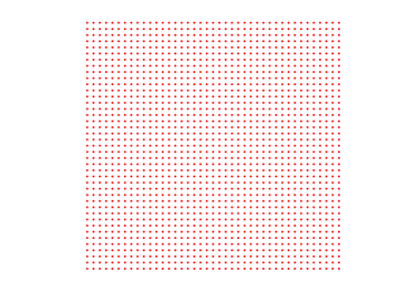
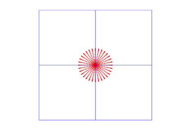
Figure 1: Two grids used in the phase (or Fourier) domain in the improved algorithm in [28]: the regular grid on the left panel is used to compute $I_{1}$ in (2.17) via the regular FFT; while the polar grid (confined in a small region centered at the origin) on the right panel is used to compute $I_{2}$ in (2.17) via the NUFFT. Note that the number of points in the polar grid is $O(1)$, thus keeping the interpolation cost in NUFFT minimal.

2.2 Numerical comparison

In this subsection, we will show the accuracy and efficiency of the NUFFT based algorithm (referred as NUFFT) for computing dipole interaction $\Phi(\mathbf{x})$ and compare them with the existing methods that applies (1.11)-(1.13) via the DST (referred as DST). To this end, we denote $\mathcal{D}$ as the computational domain, $\mathcal{D}_{h}$ as its partition with mesh size $h$ and $\Phi_{h}(\mathbf{x})$ as the numerical solution obtained on the domain $\mathcal{D}_{h}$. Hereafter, we choose $h_{x}=h_{y}=h_{z}$ in 3D and/or $h_{x}=h_{y}$ in 2D and denote them uniformly as $h$ unless stated otherwise. To demonstrate the comparison, we define the error function as

$$e_{h}:=\|\Phi-\Phi_{h}\|_{l^{2}}/\|\Phi\|_{l^{2}},$$ (2.18)

where $\|\cdot\|_{l^{2}}$ is the $l^{2}$-norm.

Example 2.1.

Dipole-dipole interaction in 3D.

In this example, we take $d=3$ and choose the source density $\rho(\mathbf{x})=e^{-|\mathbf{x}|^{2}/\sigma^{2}}$ with $\sigma>0$. The 3D dipole interaction with two dipole orientations $\mathbf{n}$ and $\mathbf{m}$ can be given explicitly as

$$\Phi(\mathbf{x})=-(\mathbf{n}\cdot\mathbf{m})\,\rho(\mathbf{x})-3\;\partial_{\mathbf{n}\mathbf{m}}\left(\frac{\sigma^{2}\sqrt{\pi}}{4}\frac{\text{Erf}(r/\sigma)}{r/\sigma}\right)=-(\mathbf{n}\cdot\mathbf{m})\,\rho(\mathbf{x})-3\;\mathbf{n}^{T}G(\mathbf{x})\mathbf{m},$$ (2.19)

where the matrix $G(\mathbf{x})=(g_{jl}(\mathbf{x}))_{j,l=1}^{3}$ is given as

$$g_{jl}(\mathbf{x})=\left(\frac{\sigma^{2}}{2r^{2}}e^{-\frac{r^{2}}{\sigma^{2}}}-\frac{\sigma^{3}\sqrt{\pi}}{4r^{3}}\text{Erf}\left(\frac{r}{\sigma}\right)\right)\delta_{jl}+x_{j}x_{l}\left(-\frac{3\;\sigma^{2}}{2\;r^{4}}e^{-\frac{r^{2}}{\sigma^{2}}}-\frac{1}{r^{2}}e^{-\frac{r^{2}}{\sigma^{2}}}+\frac{3\;\sigma^{3}\sqrt{\pi}}{4\;r^{5}}\text{Erf}\left(\frac{r}{\sigma}\right)\right),$$ (2.20)

with $\delta_{jl}$ the Kronecker delta, $\mathbf{x}=(x_{1},x_{2},x_{3})^{T}$ and $\text{Erf}(r)=\frac{2}{\sqrt{\pi}}\int_{0}^{r}e^{-s^{2}}ds$ the error function. We choose $\sigma=1.4$ and compute the potential $\Phi(\mathbf{x})$ on a uniform mesh grid, i.e., $h_{x}=h_{y}=h_{z}$ on the domain $[-L,L]^{3}$ by the DST and NUFFT methods. Table 1 shows the numerical errors $e_{h}$ via the DST and NUFFT methods with different dipole axis, i.e., $\mathbf{n}=(0.82778,0.41505,-0.37751)^{T}$ and $\mathbf{m}=(0.31180,0.93780,-0.15214)^{T}$, while Table 2 presents errors $e_{h}$ with the same dipole axis, i.e., $\mathbf{n}=\mathbf{m}=(0,0,1)^{T}$.

From Tabs. 1-2, we can clearly observe that: (i) The errors are saturated in the DST method as the mesh size $h$ tends smaller and the saturated accuracy decreases linearly with respect to the domain size $L$; (ii) The NUFFT method is spectrally accurate and it essentially does not depend on the domain, which implies that a very large bounded computational domain is not necessary in practical computations.

Table 1: Errors of the 3D dipole interaction with different axis for different $h$ and $L$.

  NUFFT h=2 $h=1$ $h=1/2$ $h=1/4$ $L=4$ 6.004E-01 6.122E-03 1.362E-04 9.823E-05 $L=8$ 6.344E-01 5.739E-03 1.189E-09 6.323E-14 $L=16$ 6.641E-01 6.054E-03 1.162E-09 1.188E-13 DST $h=1$ $h=1/2$ $h=1/4$ $h=1/8$ $L=8$ 1.985E-01 2.022E-01 2.038E-01 2.046E-01 $L=16$ 7.135E-02 7.172E-02 7.200E-02 7.214E-02 $L=32$ 2.622E-02 2.544E-02 2.549E-02 2.552E-02  

Table 2: Errors for the 3D dipole interaction with the same axis for different $h$ and $L$.

  NUFFT $h=2$ $h=1$ $h=1/2$ $h=1/4$ $L=4$ 1.118E-01 3.454E-04 1.335E-04 1.029E-04 $L=8$ 5.281E-02 3.428E-04 9.834E-12 1.601E-14 $L=16$ 5.202E-02 3.551E-04 1.143E-11 8.089E-15 DST $h=1$ $h=1/2$ $h=1/4$ $h=1/8$ $L=8$ 6.919E-02 7.720E-02 8.124E-02 8.327E-02 $L=16$ 2.709E-02 2.853E-02 2.925E-02 2.961E-02 $L=32$ 1.008E-02 1.033E-02 1.046E-02 1.052E-02  

Example 2.2.

Dipole-dipole interaction in 2D.

Here, we take $d=2$ and choose the source density as $\rho(\mathbf{x})=e^{-|\mathbf{x}|^{2}/\sigma^{2}}$ with $\sigma>0$. The exact 2D dipole interaction with two dipole orientations $\mathbf{n}_{\perp}$ and $\mathbf{m}_{\perp}$ can be given as [28]:

$$\Phi(\mathbf{x}) = \frac{3\,\sqrt{\pi}\,e^{-r}}{4\sigma}\Big{[}(\mathbf{n}_{\perp}\cdot\mathbf{m}_{\perp})(I_{0}(r)-I_{1}(r))-\frac{2\,(\mathbf{x}\cdot\mathbf{n}_{\perp})(\mathbf{x}\cdot\mathbf{m}_{\perp})}{\sigma^{2}}\Big{(}I_{0}(r)$$ (2.21)

$$-\frac{1+2\,r}{2\,r}I_{1}(r)\Big{)}\Big{]}+\frac{3\,\sqrt{\pi}\,n_{3}\,m_{3}\,r\,e^{-r}}{\sigma}\Big{[}I_{0}(r)-I_{1}(r)-\frac{I_{0}(r)}{2\,r}\Big{]},$$

where $r=\frac{|\mathbf{x}|^{2}}{2\sigma^{2}}$, $I_{0}$ and $I_{1}$ are the modified Bessel functions of order $0$ and $1$, respectively [1]. Here, we choose $\sigma=\sqrt{1.3}$ and dipole axis as $\mathbf{n}_{\perp}=(0,-0.896)^{T}$ and $\mathbf{m}_{\perp}=(0,-0.52476)^{T}$ (corresponding to $\mathbf{n}=(0,-0.896,0.44404)^{T}$ and $\mathbf{m}=(0,-0.52476,0.85125)^{T}$ in 3D). Table 3 shows the errors $e_{h}$ via the DST and NUFFT methods for different domain size $L$ and mesh size $h$.

From Tab. 3, we can clearly observe that: (i) The errors are saturated in the DST method as the mesh size $h$ tends smaller and the saturated accuracy decreases linearly with respect to the domain size $L$; (ii) The NUFFT method is spectrally accurate and it essentially does not depend on the domain if it is adequately large.

Table 3: Errors of the 2D dipole interaction by different methods with $h$ on $[-L,L]^{2}$.

  NUFFT $h=2$ $h=1$ $h=1/2$ $h=1/4$ $L=4$ 11.96 6.444E-01 5.251E-06 7.343E-06 $L=8$ 1.279 1.611E-02 4.039E-07 4.720E-14 $L=16$ 3.289E-01 1.631E-02 4.226E-08 3.489E-14 DST $h=2$ $h=1$ $h=1/2$ $h=1/4$ $L=8$ 3.200E-01 1.944E-02 1.145E-02 1.208E-02 $L=16$ 3.264E-01 1.660E-02 2.971E-03 3.048E-03 $L=32$ 3.281E-01 1.636E-02 7.590E-04 7.686E-04  

Example 2.3.

Dipole-dipole interaction for anisotropic densities.

In this example, we consider the dipole-dipole interaction for anisotropic densities which are localized in one or two spatial directions. As stated in the introduction, the 3D/2D dipole interaction (1.13) can be solved analytically via the Poisson equation (1.11) and the fractional Poisson equation (1.12) in 3D and 2D, respectively. Therefore, the dipole-dipole interaction can be obtained analytically via the solution of the Poisson/ fractional Poisson potential, followed by differentiation.

The 2D case. For an anisotropic density $\rho(x,y)=\frac{1}{4\pi\varepsilon}e^{-\frac{x^{2}}{4}-\frac{y^{2}}{4\varepsilon^{2}}}$ with a small parameter $0<\varepsilon\leq 1$, the 2D Coulomb potential (1.12) is given analytically [16] as:

$$u(x,y)=\frac{1}{2\pi\sqrt{\pi}}\int_{0}^{\infty}G(x,y,s)ds,\quad\quad G(x,y,s)=\frac{\text{exp}(-\frac{x^{2}}{4(1+s^{2})}-\frac{y^{2}}{4(s^{2}+\varepsilon^{2})})}{\sqrt{s^{2}+1}\sqrt{s^{2}+\varepsilon^{2}}}.$$ (2.22)

Then, the 2D DDI can be obtained by differentiating the integrand $G$ in (2.22). For the convenience of readers, it can be evaluated explicitly as:

$$\Phi(x,y)=-\frac{3}{4\pi^{3/2}}\!\int_{0}^{\infty}\left((n_{1}m_{1}-n_{3}m_{3})G_{xx}+(n_{2}m_{2}-n_{3}m_{3})G_{yy}+(n_{1}m_{2}+n_{2}m_{1})G_{xy}\right)ds.$$ (2.23)

Similarly as [16], to numerically evaluate (2.23), we first split it into two integrals and reformulate the one with infinite interval into an equivalent integral with finite interval by a change of variable. Then, we apply high order Gauss-Kronrod quadrature to each integral to get reference solutions. Here we omit details for brevity. With this way, we can obtain the ‘exact’ 2D DDI with the given density $\rho(x,y)$.

As discussed in [16], the 2D Coulomb interaction can be well-resolved by the NUFFT method on a heterogenous rectangle $\mathcal{D}_{\varepsilon}=[-L,L]\times[-\varepsilon L,\varepsilon L]$. The DST method, best suited for solving the PDEs with homogeneous Dirichlet boundary condition on a rectangular domain, fails to produce even a satisfactory result on $\mathcal{D}_{\varepsilon}$, mainly because the potential does not decay fast enough. Actually, the DST method can give reasonably accurate results on a square $\mathcal{D}=[-L,L]^{2}$ due to that the homogeneous Dirichlet boundary condition doesn’t bring significant error, however, one needs to resolve the anisotropic density with $h_{y}=\varepsilon h_{x}$. Then the computational and storage costs for the DST method will correspondingly scale linearly as a function of $1/\varepsilon$. Here we adapt the similar strategy for the choice of computational domains for the NUFFT and DST methods to compute the DDI. Table 4 presents errors of the 2D dipole interaction for anisotropic densities by NUFFT on $\mathcal{D}_{\varepsilon}$ and DST on $\mathcal{D}$ with $h_{x}=1/8,h_{y}=\varepsilon h_{x}$ for the same $\mathbf{n},\mathbf{m}$ as in the Example 2.2.

Table 4: Errors of the 2D dipole interaction for anisotropic densities solved on $\mathcal{D}_{\varepsilon}$ and $\mathcal{D}$ for the NUFFT and DST methods, respectively, with $h_{x}=1/8$.

  NUFFT $\varepsilon=1$ $\varepsilon=1/2$ $\varepsilon=1/4$ $\varepsilon=1/8$ $\varepsilon=1/16$ $L=8$ 3.456E-07 4.167E-07 3.984E-07 3.207E-07 2.864E-07 $L=16$ 1.005E-12 7.531E-15 5.119E-15 4.108E-15 3.720E-15 $L=32$ 2.241E-12 6.856E-15 4.913E-15 4.072E-15 3.855E-15 DST $\varepsilon=1$ $\varepsilon=1/2$ $\varepsilon=1/4$ $\varepsilon=1/8$ $\varepsilon=1/16$ $L=8$ 4.014E-02 3.182E-02 1.711E-02 6.276E-03 2.181E-03 $L=16$ 9.604E-03 7.534E-03 4.035E-03 1.479E-03 5.137E-04 $L=32$ 2.386E-03 1.868E-03 9.995E-04 3.661E-04 1.272E-04  

As for the 3D case, there are two typical kinds of anisotropic densities, that is, densities that are strongly localized in one or two directions. The first typical kind of anisotropic density is localized in one direction. For example, choose the density as $\rho(x,y,z)=\frac{1}{8\pi\sqrt{\pi}\varepsilon}e^{-\frac{x^{2}+y^{2}}{4}}e^{-\frac{z^{2}}{4\varepsilon^{2}}}$, and its corresponding 3D Coulomb potential (1.11) is given as:

$$u(x,y,z)=\frac{1}{8\pi^{3/2}}\int_{0}^{\infty}e^{-\frac{x^{2}+y^{2}}{4(1+s)}}e^{-\frac{z^{2}}{4(s+\varepsilon^{2})}}\frac{1}{(1+s)\sqrt{s+\varepsilon^{2}}}ds.$$ (2.24)

The second kind of anisotropic density is localized in two directions. For example, the density is taken as $\rho(x,y,z)=\frac{1}{8\pi\sqrt{\pi}\varepsilon^{2}}e^{-\frac{x^{2}+y^{2}}{4\varepsilon^{2}}}e^{-\frac{z^{2}}{4}}$, and the corresponding 3D Coulomb potential (1.11) is given analytically as:

$$u(x,y,z)=\frac{1}{8\pi^{3/2}}\int_{0}^{\infty}e^{-\frac{x^{2}+y^{2}}{4(s+\varepsilon^{2})}}e^{-\frac{z^{2}}{4(s+1)}}\frac{1}{\sqrt{1+s}\;(s+\varepsilon^{2})}ds.$$ (2.25)

Similarly as in the 2D case, the DDI in 3D can be obtained by differentiating the integrand in (2.24) and (2.25). They can be evaluated numerically in a similar way, which can be viewed as the ‘exact’ solution. For brevity, we omit the formulas and relevant details.

To numerically compute the 3D dipole interaction by the NUFFT and DST methods, we shall adopt the meshing strategy, i.e., $h_{y}=h_{x}$ and $h_{z}=\varepsilon h_{x}$ for densities localized only in $z$-direction and $h_{y}=h_{x}=\varepsilon h_{z}$ for densities localized in $x,y$ directions. Similarly, the NUFFT method is applied on a heterogenous cube $\mathcal{D}_{\varepsilon}=[-L,L]^{2}\times[-\varepsilon L,\varepsilon L]$ or $[-\varepsilon L,\varepsilon L]^{2}\times[-L,L]$. The DST method is used on $\mathcal{D}=[-L,L]^{3}$ so that the homogeneous Dirichlet boundary condition doesn’t bring significant error. Correspondingly, the computational and storage costs of the DST method will scale linearly as a function of $1/\varepsilon$ (the first kind) or $1/\varepsilon^{2}$ (the second kind).

To show the accuracy performance of both methods, we take the first kind density as the test function (2.24). Here we take the same dipole axis $\mathbf{n}=\mathbf{m}=(0,0,1)^{T}$ for simplicity. Table 5 presents errors of the 3D dipole interaction for anisotropic densities localized in the $z$-direction by NUFFT on $\mathcal{D}_{\varepsilon}$ and DST on $\mathcal{D}$ with $h_{x}=1/4$ and $h_{z}=\varepsilon h_{x}$.

Table 5: Errors of the 3D dipole interaction (2.24) by NUFFT on $\mathcal{D}_{\varepsilon}$ and DST on $\mathcal{D}$ with $h_{x}=1/4$ and $\mathbf{n}=\mathbf{m}=(0,0,1)^{T}$.

  NUFFT $\varepsilon=1$ $\varepsilon=1/2$ $\varepsilon=1/4$ $\varepsilon=1/8$ $\varepsilon=1/16$ $L=8$ 3.004E-08 2.581E-08 2.307E-08 1.988E-08 1.578E-08 $L=16$ 1.598E-14 7.590E-15 4.590E-15 2.184E-15 1.193E-15 DST $\varepsilon=1$ $\varepsilon=1/2$ $\varepsilon=1/4$ $\varepsilon=1/8$ $\varepsilon=1/16$ $L=8$ 1.409E-01 7.667E-02 4.308E-02 2.633E-02 1.716E-02 $L=16$ 5.003E-02 2.754E-02 1.548E-02 9.453E-03 6.159E-03 $L=32$ 1.786E-02 9.836E-03 5.522E-03 3.370E-03 2.195E-03  

From Tabs. 4-5, we can conclude: (1) the NUFFT can evaluate accurately the 2D and 3D dipole interaction with anisotropic densities. (2) The DST method can still capture satisfactory results if the computational domain is large enough, however, the computational and storage costs increase when the heterogeneity of the density increases, which makes it less applicable, especially in 3D simulation.

3 Ground state computation

In this section, we propose an efficient and accurate numerical method for computing the ground state by combining the normalized gradient flow which is discretized by the backward Euler Fourier pseudospectral method and the NUFFT nonlocal DDI interaction solver. We shall refer to this new method as GF-NUFFT hereafter. The spatial spectral accuracy is investigated in details, the virial identity is verified numerically, with comparison to some existing results in [8], to show the advantage of the GF-NUFFT method in term of accuracy.

3.1 A numerical method via the NUFFT

Let $\Delta t>0$ be the time step and denote $t_{n}=n\Delta t$ for $n=0,1,2,\ldots$  . Many efficient and accurate numerical methods have been proposed for computing the ground state of the GPE [8, 9, 10, 49]. One of the most simple and successful method is by solving the following gradient flow with discretized normalization (GFDN):

$$\partial_{t}\phi(\mathbf{x},t)=\left[\frac{1}{2}\nabla^{2}-V(\mathbf{x})-\beta|\psi|^{2}-\lambda\,\Phi(\mathbf{x},t)\right]\phi(\mathbf{x},t),\quad\mathbf{x}\in{\mathbb{R}}^{d},\quad t_{n}\leq t<t_{n+1},$$ (3.26)

$$\Phi(\mathbf{x},t)=\left(U_{\rm dip}\ast|\phi|^{2}\right)(\mathbf{x},t),\;\;\;\quad\quad\qquad\qquad\qquad\qquad\mathbf{x}\in{\mathbb{R}}^{d},\quad t_{n}\leq t<t_{n+1},$$ (3.27)

$$\phi(\mathbf{x},t_{n+1})=\frac{\phi(\mathbf{x},t_{n+1}^{-})}{\|\phi(\mathbf{x},t_{n+1}^{-})\|},\qquad\quad\qquad\qquad\qquad\qquad\mathbf{x}\in{\mathbb{R}}^{d},\quad n\geq 0,$$ (3.28)

with the initial data

$$\phi(\mathbf{x},0)=\phi_{0}(\mathbf{x}),\qquad\mathbf{x}\in{\mathbb{R}}^{d},\qquad{\rm with}\qquad\|\phi_{0}\|^{2}:=\int_{{\mathbb{R}}^{d}}|\phi_{0}(\mathbf{x})|^{2}\,d\mathbf{x}=1.$$ (3.29)

Let $\phi^{n}(\mathbf{x})$ and $\Phi^{n}(\mathbf{x})$ be the numerical approximations of $\phi(\mathbf{x},t_{n})$ and $\Phi(\mathbf{x},t_{n})$, respectively, for $n\geq 0$. The above GFDN is usually discretized in time via the backward Euler method [8, 49]

$$\frac{\phi^{(1)}(\mathbf{x})-\phi^{n}(\mathbf{x})}{\Delta t}=\left[\frac{1}{2}\nabla^{2}-V(\mathbf{x})-\beta|\psi^{n}|^{2}-\lambda\,\Phi^{n}(\mathbf{x})\right]\phi^{(1)}(\mathbf{x}),\qquad\mathbf{x}\in{\mathbb{R}}^{d},$$ (3.30)

$$\Phi^{n}(\mathbf{x})=\left(U_{\rm dip}\ast|\phi^{n}|^{2}\right)(\mathbf{x}),\quad\qquad\qquad\qquad\qquad\quad\qquad\qquad\;\;\,\mathbf{x}\in{\mathbb{R}}^{d},$$ (3.31)

$$\phi^{n+1}(\mathbf{x})=\frac{\phi^{(1)}(\mathbf{x})}{\|\phi^{(1)}(\mathbf{x})\|},\quad\qquad\qquad\qquad\qquad\qquad\qquad\mathbf{x}\in{\mathbb{R}}^{d},\quad n\geq 0.$$ (3.32)

As it is known, the ground state decays exponentially fast due to the trapping potential, therefore, in practical computations, we shall first truncate the whole space to a bounded domain $\mathcal{D}$ and impose periodic boundary conditions. It is worthwhile to point out that the dipole interaction is originally defined by convolution, therefore it does not require any boundary condition. Then, the equation (3.30) is discretized in space via the Fourier pseudospectral method and the dipole interaction $\Phi^{n}(\mathbf{x})$ in (3.31) is evaluated by the NUFFT solver. The initial guess $\phi_{0}(\mathbf{x})$ is usually chosen as a positive function, e.g., a Gaussian, and the ground state $\phi_{g}(\mathbf{x})$ is obtained numerically as $\phi^{n}(\mathbf{x})$ once $\frac{\|\phi^{n}(\mathbf{x})-\phi^{n+1}(\mathbf{x})\|_{l^{\infty}}}{\Delta t}\leq\varepsilon_{0}$ is satisfied, where $\varepsilon_{0}$ is the desired accuracy. The details are omitted here for brevity.

3.2 Numerical results

In order to study the spatial accuracy of the GF-NUFFT method for computing the ground state, we denote $\Phi_{g}(\mathbf{x})=(U_{\rm dip}\ast|\phi_{g}|^{2})(\mathbf{x})$ and introduce the error functions

$$e_{\phi_{g}}^{h}:=\frac{\|\phi_{g}(\mathbf{x})-\phi_{g}^{h}(\mathbf{x})\|_{l^{2}}}{\|\phi_{g}(\mathbf{x})\|_{l^{2}}},\qquad e_{\Phi_{g}}^{h}:=\frac{\|\Phi_{g}(\mathbf{x})-\Phi_{g}^{h}(\mathbf{x})\|_{l^{2}}}{\|\Phi_{g}(\mathbf{x})\|_{l^{2}}},$$

where $\phi_{g}^{h}$ and $\Phi_{g}^{h}$ are obtained numerically by a numerical method with the mesh size $h$. Additionally, we split the energy functional into four parts

$$E(\phi)=E_{\rm kin}(\phi)+E_{\rm pot}(\phi)+E_{\rm int}(\phi)+E_{\rm dip}(\phi),$$

where the kinetic energy $E_{\rm kin}(\phi)$, the potential energy $E_{\rm pot}(\phi)$, the interaction energy $E_{\rm int}(\phi)$, and the dipole interaction energy $E_{\rm dip}(\phi)$ are defined as

$$E_{\rm kin}(\phi)=\frac{1}{2}\int_{\mathbb{R}^{d}}|\nabla\phi(\mathbf{x})|^{2}d\mathbf{x},\quad E_{\rm pot}(\phi)=\int_{\mathbb{R}^{d}}V(\mathbf{x})|\phi(\mathbf{x})|^{2}d\mathbf{x},$$

$$E_{\rm int}(\phi)=\frac{\beta}{2}\int_{\mathbb{R}^{d}}|\phi(\mathbf{x})|^{4}d\mathbf{x},\qquad E_{\rm dip}(\phi)=\frac{\lambda}{2}\int_{\mathbb{R}^{d}}\Phi(\mathbf{x})|\phi(\mathbf{x})|^{2}d\mathbf{x},$$

respectively. Moreover, the chemical potential can be reformulated as $\mu(\phi)=E(\phi)+E_{\rm int}(\phi)+E_{\rm dip}(\phi)$. Furthermore, if the external potential $V(\mathbf{x})$ in (1.1) is taken as the harmonic potential (1.4) [7, 15, 16, 36], the energies of the ground state satisfy the following virial identity

$$0=I:=2E_{\rm kin}(\phi_{g})-2E_{\rm pot}(\phi_{g})+3E_{\rm int}(\phi_{g})+3E_{\rm dip}(\phi_{g}).$$ (3.33)

We denote $I^{h}$ as an approximation of $I$ when $\phi_{g}$ and $\Phi_{g}$ are replaced by $\phi_{g}^{h}$ and $\Phi_{g}^{h}$ in (3.33). In our computations, the ground state $\phi_{g}^{h}$ is reached numerically when $\frac{\|\phi^{n+1}(\mathbf{x})-\phi^{n}(\mathbf{x})\|_{l^{\infty}}}{\Delta t}\leq\varepsilon_{0}$ with $\varepsilon_{0}=10^{-10}$. The initial data $\phi_{0}(\mathbf{x})$ is chosen as a Gaussian and the time step is taken as $\Delta t=10^{-2}$. In the comparisons, the “exact” solution $\phi_{g}(\mathbf{x})$ was obtained numerically via the GF-NUFFT method on a large enough domain $\Omega$ with small enough mesh size $h$ and the same time step $\Delta t=10^{-2}$.

Table 6: Errors of the ground states and the dipole interaction obtained by the GF-NUFFT method for $\mathbf{n}=(0,0,1)^{T}$ and $\beta=200$ with different mesh sizes $h$ and $\lambda$.

  GF-NUFFT $h=2$ $h=1$ $h=1/2$ $h=1/4$ $h=1/8$ $e^{h}_{\phi_{g}}$ $\lambda=-100\;$ 1.783E-02 3.102E-03 3.463E-05 3.652E-09 4.133E-12 $\lambda=\;\;100\;$ 1.263E-02 2.717E-03 3.599E-05 6.183E-09 2.841E-12 $\lambda=\;\;200\;$ 1.670E-02 3.049E-03 8.897E-05 5.364E-08 3.871E-12 $e^{h}_{\Phi_{g}}$ $\lambda=-100\;$ 2.810E-02 3.683E-03 1.842E-05 1.555E-09 8.132E-12 $\lambda=\;\;100\;$ 2.385E-02 4.932E-03 9.445E-05 1.996E-08 2.750E-12 $\lambda=\;\;200\;$ 1.406E-02 5.681E-03 2.424E-04 1.921E-07 3.121E-12  

Accuracy confirmation. To show the accuracy of the GF-NUFFT, we take $d=3$, $\mathbf{n}=(0,0,1)^{T}$, $\beta=200$ and $V(\mathbf{x})=\frac{1}{2}(x^{2}+y^{2}+z^{2}/4)$. Table 6 presents errors of the ground states and the corresponding dipole interactions computed on a fixed domain $[-8,8]^{3}$ with different mesh sizes and $\lambda$. From this Table, we can observe clearly the spectral convergence in space of the GF-NUFFT method.

Virial identity. Here we take the same physical parameters as used in [8] (cf. Table 3), i.e., $d=3$, $\beta=207.16$ and $V(\mathbf{x})=\frac{1}{2}(x^{2}+y^{2}+z^{2}/4)$. We compute the ground state on a larger domain, i.e., $[-12,12]^{3}$, with a coarser mesh size $h_{x}=h_{y}=h_{z}=1/4$. Different energies of the ground state and related quantities are shown in Table 7. Compared with Table 3 in [8] where the identity is only accurate up to 3 significant digits, our results by the GF-NUFFT method agree quite well with the identity, up to 9 significant digits.

Table 7: Different energies of the ground state and $I^{h}$ for the 3D dipolar BEC with $\beta=207.16$ for different $\lambda$.

  $\lambda$ $E_{g}$ $\mu_{g}$ $E_{\textrm{kin}}^{g}$ $E_{\textrm{pot}}^{g}$ $E_{\textrm{int}}^{g}$ $E_{\textrm{dip}}^{g}$ $I^{h}$ $-103.58$ 2.9584 3.9301 0.26466 1.7221 0.83892 0.13273 6.6214E-10 $-51.79$ 2.8841 3.8187 0.27379 1.6757 0.85255 0.082056 5.7861E-10 $0$ 2.7943 3.6830 0.28621 1.6193 0.88875 0.0000 5.0929E-10 $51.79$ 2.6875 3.5201 0.30303 1.5519 0.94903 -0.11646 4.5134E-10 $103.58$ 2.5593 3.3213 0.32704 1.4701 1.0451 -0.28304 3.6672E-10 $155.37$ 2.3998 3.0674 0.36538 1.3668 1.2105 -0.54290 2.3288E-10 $207.16$ 2.1838 2.7011 0.44525 1.2212 1.5749 -1.0576 -1.6697E-10  

4 Dynamics simulation

In this section, instead of solving the GPE (1.1)-(1.3), we consider a more general GPE in $d$-dimensions ($d=2,3$) with both the damping term and time (in-)dependent DDI:

$$i\partial_{t}\psi({\mathbf{x}},t)=\left[-\frac{1}{2}\nabla^{2}+V({\bf x})+\beta|\psi|^{2\sigma}+\lambda\Phi(\mathbf{x},t)-if(|\psi|^{2})\right]\psi(\mathbf{x},t),$$ (4.34)

$$\Phi(\mathbf{x},t)=(U_{\rm dip}\ast|\psi|^{2})(\mathbf{x},t),\qquad\mathbf{x}\in{\mathbb{R}}^{d},\qquad t\geq 0,$$ (4.36)

$$\psi(\mathbf{x},t=0)=\psi_{0}(\mathbf{x}).$$

Here, $\sigma>0$ corresponds to the type of the nonlinearity ($\sigma=1$ represents to the cubic nonlinearity, and resp., $\sigma=2$ to a quintic nonlinearity). $f(\rho)\geq 0$ for $\rho=|\psi|^{2}\geq 0$ is a real-valued monotonically increasing function that represents the type of damping. In BEC, when $f(\rho)\equiv 0$, (4.34) reduces to the usual GPE (1.1) without damping effect, while a linear damping term $f(\rho)\equiv\delta$ with $\delta>0$ represents inelastic collisions with the background gas. In addition, the cubic damping $f(\rho)=\delta_{1}\rho$ with $\delta_{1}>0$ describes two-body loss, a quintic damping term of the form $f(\rho)=\delta_{2}\rho^{2}$ with $\delta_{2}>0$ corresponds to the three-body loss, and their combination $f(\rho)=\delta_{1}\rho+\delta_{2}\rho^{2}$ takes both the two and three-body loss into account. Furthermore, the kernel of the dipole interaction may be time (in-)dependent, which is defined as

$$U_{\rm dip}(\mathbf{x},t) = \frac{3}{4\pi}\frac{\mathbf{m}(t)\cdot\mathbf{n}(t)-3(\mathbf{x}\cdot\mathbf{m}(t))(\mathbf{x}\cdot\mathbf{n}(t))/|\mathbf{x}|^{2}}{|\mathbf{x}|^{3}}$$

$$= -(\mathbf{m}(t)\cdot\mathbf{n}(t))\delta(\mathbf{x})-3\partial_{\mathbf{m}(t)\mathbf{n}(t)}\left(\frac{1}{4\pi|\mathbf{x}|}\right),\qquad\mathbf{x}\in{\mathbb{R}}^{3},$$

where $\mathbf{m}(t)=(m_{1}(t),m_{2}(t),m_{3}(t))^{T}$ and $\mathbf{n}(t)=(n_{1}(t),n_{2}(t),n_{3}(t))^{T}\in{\mathbb{R}}^{3}$ are two given time (in-)dependent unit vectors, representing the two dipole orientations. The energy is modified as:

$$\mathcal{E}(t) =: \int_{{\mathbb{R}}^{d}}\Big{[}\frac{1}{2}|\nabla\psi|^{2}+V({\bf x})|\psi|^{2}+\frac{\beta}{\delta+1}|\psi|^{2\,(\delta+1)}+\frac{\lambda}{2}\Phi(\mathbf{x},t)\,|\psi|^{2}$$ (4.38)

$$-\frac{\lambda}{2}\int_{0}^{t}\Big{(}\partial_{s}U_{\rm dip}\ast|\psi|^{2}\Big{)}|\psi(\mathbf{x},s)|^{2}ds\Big{]}d{\bf x},$$

which satisfies the following dynamical law:

$$\frac{d}{dt}\mathcal{E}(t)=-2\int_{{\mathbb{R}}^{d}}f(|\psi|^{2}){\rm Im}\big{(}\psi\partial_{t}\overline{\psi}\big{)}d\mathbf{x}.$$ (4.39)

where $\overline{\psi}$ denotes the complex conjugate of $\psi$. The total mass $N(t)$ (1.7) is dissipated as:

$$\frac{d}{dt}N(t)=-2\int_{{\mathbb{R}}^{d}}f(|\psi|^{2})|\psi|^{2}d\mathbf{x}.$$ (4.40)

We will present an accurate and efficient numerical method for simulating the dynamics of the GPE (4.34)-(4.36). The method incorporates the NUFFT solver for the evaluation of the nonlocal dipole interaction and the time-splitting Fourier pseudospectral discretization for the GPE (4.34).

4.1 Numerical method

In practical computation, we first truncate the problem (4.34)-(4.36) into a bounded computational domain $\mathcal{D}=[L_{x},R_{x}]\times[L_{y},R_{y}]\times[L_{z},R_{z}]$ if $d=3$, or $\mathcal{D}=[L_{x},R_{x}]\times[L_{y},R_{y}]$ if $d=2$. From $t=t_{n}$ to $t=t_{n+1}$, the GPE (4.34) will be solved in two steps. One first solves

$$i\partial_{t}\psi(\mathbf{x},t)=-\frac{1}{2}\nabla^{2}\psi(\mathbf{x},t),\qquad\quad\mathbf{x}\in{\mathcal{D}},\qquad t_{n}\leq t\leq t_{n+1},$$ (4.41)

with periodic boundary condition on the boundary $\partial\mathcal{D}$ for a time step of length $\Delta t$, followed by solving

$$i\partial_{t}\psi({\mathbf{x}},t) = \left[V({\bf x})+\beta|\psi|^{2\sigma}+\lambda\Phi(\mathbf{x},t)-if(|\psi|^{2})\right]\psi(\mathbf{x},t),\qquad\mathbf{x}\in\mathcal{D},\quad t_{n}\leq t\leq t_{n+1},\qquad$$ (4.42)

$$\Phi(\mathbf{x},t) = \big{(}U_{\rm dip}\ast|\psi|^{2}\big{)}(\mathbf{x},t),\qquad\qquad\quad\mathbf{x}\in\mathcal{D},\quad t_{n}\leq t\leq t_{n+1},$$ (4.43)

for the same time step. The linear subproblem (4.41) will be discretized in space by the Fourier pseudospectral method and integrated in time exactly in the phase space, while the nonlinear subproblem (4.42)-(4.43) can be integrated exactly, one can refer to [8, 14, 11, 13] for details. To simplify the presentation, we will only present the scheme for the 3D case. As for the 2D case, one can modify the algorithm straightforward.

Let $L$, $M$, $N$ be even positive integers, choose $h_{x}=\frac{R_{x}-L_{x}}{L}$, $h_{y}=\frac{R_{y}-L_{y}}{M}$ and $h_{z}=\frac{R_{z}-L_{z}}{N}$ as the spatial mesh sizes in $x$-, $y$-, and $z$- directions, respectively. Define the index and grid points sets as

$${\mathcal{T}}_{LMN} = \left\{(l,k,m)\,|\,0\leq l\leq L,\ 0\leq k\leq M,\ 0\leq m\leq N\right\},$$

$$\widetilde{\mathcal{T}}_{LMN} = \left\{(p,q,r)\,|\,-\frac{L}{2}\leq p\leq\frac{L}{2}-1,\ -\frac{M}{2}\leq q\leq\frac{M}{2}-1,\ -\frac{N}{2}\leq r\leq\frac{N}{2}-1\right\},$$

$${\mathcal{G}}_{xyz} = \left\{(x_{l},y_{k},z_{m})=:(L_{x}+jh_{x},L_{y}+kh_{y},L_{z}+mh_{z}),\ (l,k,m)\in{\mathcal{T}}_{LMN}\right\}.$$

Define the functions

$$W_{pqr}^{s}(x,y,z)=e^{i\mu_{p}^{x}(x-L_{x})}\,e^{i\mu_{q}^{y}(y-L_{y})}\,e^{i\mu_{r}^{z}(z-L_{z})},\quad(p,q,r)\in\widetilde{\mathcal{T}}_{LMN},$$

with

$$\mu_{p}^{x}=\frac{2p\pi}{R_{x}-L_{x}},\;\;\mu_{q}^{y}=\frac{2q\pi}{R_{y}-L_{y}},\;\;\mu_{r}^{z}=\frac{2r\pi}{R_{z}-L_{z}},\quad(p,q,r)\in\widetilde{\mathcal{T}}_{LMN}.$$

Let $\psi_{lkm}^{n}$ be the approximation of $\psi(x_{l},y_{k},z_{m},t_{n})$ for $(l,k,m)\in{\mathcal{T}}_{LMN}$ and $n\geq 0$ and denote $\psi^{n}$ be the solution vector at time $t=t_{n}$ with components $\{\psi_{lkm}^{n},\ (l,k,m)\in{\mathcal{T}}_{LMN}\}$. Taking the initial data as $\psi_{lkm}^{0}=\psi_{0}(x_{l},y_{k},z_{m})$ for $(l,k,m)\in{\mathcal{T}}_{LMN}$, for $n\geq 0$, a second-order time splitting Fourier pseudospectral (TSFP) method to solve the GPE (4.34)-(4.36) reads as:

$$\psi_{lkm}^{(1)} = \sum_{p=-L/2}^{L/2-1}\sum_{q=-M/2}^{M/2-1}\sum_{r=-N/2}^{N/2-1}e^{-\frac{i\Delta t}{4}\left[(\mu_{p}^{x})^{2}+(\mu_{q}^{y})^{2}+(\mu_{r}^{z})^{2}\right]}\widehat{(\psi^{n})}_{pqr}\;W_{pqr}^{s}(x_{l},y_{k},z_{m}),$$

$$\psi_{lkm}^{(2)} = \psi_{lkm}^{(1)}\exp\left\{-i\left[\Delta tV(\mathbf{x})+H(|\psi_{lkm}^{(1)}|^{2},\Delta t)+G(|\psi^{(1)}|^{2},t^{n},t^{n+1})(x_{l},y_{k},z_{m})\right]\right\}$$

$$\qquad\qquad\times\exp\{-F(|\psi_{lkm}^{(1)}|^{2},\Delta t)\},\qquad(l,k,m)\in{\mathcal{T}}_{LMN},$$

$$\psi_{lkm}^{n+1} = \sum_{p=-L/2}^{L/2-1}\sum_{q=-M/2}^{M/2-1}\sum_{r=-N/2}^{N/2-1}e^{-\frac{i\Delta t}{4}\left[(\mu_{p}^{x})^{2}+(\mu_{q}^{y})^{2}+(\mu_{r}^{z})^{2}\right]}\widehat{(\psi^{(2)})}_{pqr}\;W_{pqr}^{s}(x_{l},y_{k},z_{m}).$$ (4.44)

Here, $\widehat{(\psi^{n})}_{pqr}$ and $\widehat{(\psi^{(2)})}_{pqr}$ are the discrete Fourier transform coefficients of the vectors $\psi^{n}$ and $\psi^{(2)}$, respectively, and the functions $H(\varphi,s)$, $G(\varphi,s,s_{1})$ and $F(\varphi,s)$ are defined as:

$$H(\varphi,s)=\beta\int_{0}^{s}\left[h(\varphi,\tau)\right]^{\sigma}d\tau,\qquad F(\varphi,s)=\int_{0}^{s}f(h(\varphi,\tau))d\tau,$$ (4.45)

$$G(\varphi,s,s_{1})(\mathbf{x})=\lambda\int_{s}^{s_{1}}\left(U_{\rm dip}(\cdot,\tau)\ast h(\varphi(\cdot,\tau-s)\right)(\mathbf{x})d\tau,$$ (4.46)

with

$$h(\varphi,s)=\left\{\begin{array}[]{cc}g^{-1}(g(\varphi)-2s),&\varphi>0,\quad s\geq 0,\\ 0,&\varphi=0,\quad s\geq 0,\end{array}\right.\qquad g(s)=\int\frac{1}{sf(s)}.$$ (4.47)

For a given damping function $f(s)$, in general, $g^{-1}(s)$ and thus $h(\varphi,s)$ may not have explicit expressions. In practical computation, one could solve $h(\varphi,s)$ numerically from an auxiliary ODE, and then evaluate (4.45)-(4.46) via a numerical quadrature. For details, one can refer to Remark 2.1 in [11]. However, if the dipole axis is time independent, i.e., $U_{\rm dip}(\mathbf{x},t)\equiv U_{\rm dip}(\mathbf{x},t=0)=:U_{\rm dip}^{0}(\mathbf{x})$, for those damping terms that are frequently used in the physics literatures, the functions $H$, $F$ and $G$ can be integrated analytically. For the convince of the reader, we list them here briefly [11]:

• Case I. $f(\rho)\equiv 0$, i.e., no damping term, we have

  $$H(\varphi,s)=\beta\varphi^{\sigma}s,\qquad F(\varphi,s)=0,\qquad G(\varphi,s,s_{1})(\mathbf{x})=\lambda(s_{1}-s)\,\left(U_{\rm dip}^{0}\ast\varphi\right)(\mathbf{x}).$$

• Case II. $f(\rho)=\delta>0$, i.e., the linear damping, we have

  $$H(\varphi,s)=\frac{\beta\varphi^{\sigma}}{2\delta\sigma}\left(1-e^{-2\delta\sigma s}\right),\qquad F(\varphi,s)=\delta s,$$

  $$G(\varphi,s,s_{1})(\mathbf{x})=\frac{\lambda}{2\delta}\left(1-e^{-2\delta(s_{1}-s)}\right)\left(U_{\rm dip}^{0}\ast\varphi\right)(\mathbf{x}).$$

• Case III. $f(\rho)=\delta\rho^{q}$ with $\delta,q>0$, which corresponds to two ($q=1$) or three ($q=2$) body loss of particles, we have

  $$F(\varphi,s)=\frac{1}{2q}\ln(1+2q\delta s\varphi^{q}),$$

  $$H(\varphi,s)=\left\{\begin{array}[]{ll}\frac{\beta}{2q\delta}\ln(1+2q\delta s\varphi^{q}),&\quad{\rm if}\quad\sigma=q,\\[3.99994pt] \frac{\beta\varphi^{\sigma-q}}{2\delta(q-\sigma)}\left[\left(1+2q\delta s\varphi^{q}\right)^{1-\sigma/q}-1\right],&\quad{\rm if}\quad\sigma\neq q,\end{array}\right.$$ (4.50)

  $$G(\varphi,s,s_{1})(\mathbf{x})=\lambda\,U_{\rm dip}^{0}\ast\left\{\begin{array}[]{ll}\frac{1}{2\delta}\ln(1+2\delta(s_{1}-s)\varphi),&\quad{\rm if}\quad q=1,\\[3.99994pt] \frac{\left(1+2q\delta(s_{1}-s)\varphi^{q}\right)^{1-1/q}-1}{2\delta(q-1)\varphi^{q-1}},&\quad{\rm if}\quad q\neq 1.\end{array}\right.$$ (4.53)

The function $G$ is evaluated by the algorithm via the NUFFT as discussed in previous sections, and this method for discretizing the GPE (4.34)-(4.36) is referred as TS-NUFFT.

4.2 Test of the accuracy

In this section, we first test the accuracy of our numerical method for computing the dynamics of the dipolar BEC. To demonstrate the results, we define the following error function

$$e_{\psi}^{h,\,\Delta t}(t_{n}):=\frac{\|\psi(\mathbf{x},t_{n})-\psi^{n}_{h,\,\Delta t}(\mathbf{x})\|_{l^{2}}}{\|\psi(\mathbf{x},t)\|_{l^{2}}},\qquad n\geq 0,$$ (4.54)

where $\|\cdot\|_{l^{2}}$ represents the $l^{2}$ norm, $\psi^{n}_{h,\,\Delta t}(\mathbf{x})$ is the numerical approximation of $\psi(\mathbf{x},t=t_{n})$ obtained by the TS-NUFFT method (4.44) with mesh size $h$ and time step $\Delta t$. In this subsection, all examples are carried out for dipolar BEC without damping effect, i.e., $f(\rho)\equiv 0$ in the GPE (4.34). Moreover, the computational domain $\mathcal{D}$, the trapping potential $V(\mathbf{x})$ and the initial data $\psi_{0}(\mathbf{x})$ are respectively chosen as

$$\mathcal{D}=[-2^{6-d},2^{6-d}]^{d},\quad V(\mathbf{x})=\frac{|\mathbf{x}|^{2}}{2},\quad\psi_{0}(\mathbf{x})=\frac{1}{\sqrt[4]{\pi^{d}}}e^{-\frac{|\mathbf{x}|^{2}}{2}},\quad\mathbf{x}\in\mathcal{D}\;\;{\rm with}\;\;d=2\;\;{\rm or}\;\;3.$$ (4.55)

Furthermore, the dipole orientations are chosen as $\mathbf{n}=\mathbf{m}=(0,0,1)^{T}$ in 3D and $\mathbf{n}_{\perp}=\mathbf{m}_{\perp}=(1,0)^{T}$ in 2D, respectively.

Table 8: Spatial errors (upper parts) $e_{\psi}^{h,\,\Delta t_{0}}(t)$ and temporal errors (lower parts) $e_{\psi}^{h_{0},\,\Delta t}(t)$ at $t=0.28$ for the dynamics of the 3D GPE (4.34) with different $\beta$ and $\lambda=\frac{\beta}{2}$.

  $e_{\psi}^{h,\,\Delta t_{0}}(t)$ $h=1/2$ $h=1/4$ $h=1/8$ $h=1/16$ $\beta=2$ 3.999E-03 1.612E-05 1.601E-11 3.049E-12 $\beta=10$ 1.773E-02 2.581E-04 8.899E-09 3.133E-12 $\beta=50$ 8.074E-02 8.186E-03 2.460E-05 2.304E-11 $e_{\psi}^{h_{0},\,\Delta t}(t)$ $\Delta t=0.008$ $\Delta t/2$ $\Delta t/4$ $\Delta t/8$ $\beta=2$ 2.983E-06 7.454E-07 1.860E-07 4.615E-08 rate – 2.001 2.003 2.011 $\beta=10$ 8.151E-06 2.036E-06 5.081E-07 1.261E-07 rate – 2.001 2.003 2.011 $\beta=50$ 8.427E-05 2.105E-05 5.251E-06 1.303E-06 rate – 2.001 2.003 2.011  

Example 4.1.

Numerical accuracy verification in 3D.

Here d=3 and the “exact” solution $\psi(\mathbf{x},t)$ is obtained numerically via the TS-NUFFT method on domain $\mathcal{D}$ with very small mesh size $h=h_{0}:=\frac{1}{16}$ and time step $\Delta t=\Delta t_{0}:=10^{-4}$. Table 8 lists the spatial discretization errors $e_{\psi}^{h,\,\Delta t_{0}}(t)$ and the temporal discretization errors $e_{\psi}^{h_{0},\,\Delta t}(t)$ as well as the convergence rate at time $t=0.28$ with different mesh size $h$ and different time step $\Delta t$, for different $\beta$ and $\lambda=\frac{\beta}{2}$.

Example 4.2.

Numerical accuracy verification in 2D.

Here d=2 and the “exact” solution $\psi(\mathbf{x},t)$ is obtained numerically via the TS-NUFFT method on domain $\mathcal{D}$ with very small mesh size $h=h_{0}:=\frac{1}{32}$ and time step $\Delta t=\Delta t_{0}:=10^{-4}$. Table 9 shows the spatial discretization errors $e_{\psi}^{h,\,\Delta t_{0}}(t)$ and the temporal discretization errors $e_{\psi}^{h_{0},\,\Delta t}(t)$ as well as the convergence rate at time $t=1.0$ with different mesh size $h$ and different time step $\Delta t$, for different $\beta$ and $\lambda=\frac{\beta}{20}$.

Table 9: Spatial errors (upper parts) $e_{\psi}^{h,\,\Delta t_{0}}(t)$ and temporal errors (lower parts) $e_{\psi}^{h_{0},\,\Delta t}(t)$ at $t=1.0$ for the dynamics of the 2D GPE (4.34) with different $\beta$ and $\lambda=\frac{\beta}{20}$.

  $e_{\psi}^{h,\,\Delta t_{0}}(t)$ $h=1/2$ $h=1/4$ $h=1/8$ $h=1/16$ $\beta=2$ 5.715E-05 6.193E-11 1.120E-11 1.124E-11 $\beta=10$ 1.894E-03 6.616E-08 1.354E-11 1.679E-11 $\beta=50$ 7.265E-02 2.987E-04 4.987E-10 2.852E-11 $e_{\psi}^{h_{0},\,\Delta t}(t)$ $\Delta t=0.01$ $\Delta t/2$ $\Delta t/4$ $\Delta t/8$ $\beta=2$ 9.011E-06 2.252E-06 5.623E-07 1.399E-07 rate – 2.001 2.002 2.007 $\beta=10$ 2.293E-05 5.728E-06 1.430E-06 3.558E-07 rate – 2.001 2.002 2.007 $\beta=50$ 2.453E-04 6.122E-05 1.528E-05 3.802E-06 rate – 2.003 2.002 2.007  

From Tabs. 8-9, we can see that the TS-NUFFT method (4.44) is spectrally accurate in space and second order accurate in time for computing the dynamics of dipolar BEC.

4.3 Applications

In this section, we apply the TS-NUFFT method (4.44) to study some interesting phenomena, such as the dynamics of a BEC with time-dependent dipole orientations and the collapse and explosion of a dipolar BEC with attractive interaction and damping terms.

Example 4.3.

Dynamics of a BEC with rotating dipole orientations.

Here d=3 and we consider the GPE (4.34) without damping term, i.e., $f(\rho)\equiv 0$. The trapping potential is chosen as $V(\mathbf{x})=\frac{|\mathbf{x}|^{2}}{2}$ and the initial data in (4.36) is chosen as $\psi_{0}(\mathbf{x})=\phi_{\rm gs}(\mathbf{x})$, where $\phi_{\rm gs}(\mathbf{x})$ is the ground state of the GPE (4.34) with $f(\rho)\equiv 0$ and $\mathbf{n}=\mathbf{m}=(0,0,1)^{T},$ $\beta=103.58$ and $\lambda=82.864$, which is computed numerically via the numerical method presented in the previous section. The computational domain and mesh size are chosen as $\mathcal{D}=[-8,8]^{3}$ and $h_{x}=h_{y}=h_{z}=\frac{1}{8}$, respectively. Then we tune the dipole orientations as

$$\mathbf{n}(t)=\left(\sin\frac{t}{5},0,\cos\frac{t}{5}\right)^{T},\qquad t\geq 0,$$ (4.56)

and study the dynamics of the BEC in two cases:

• Case 1. tune the dipole orientation as in (4.56) and keep all the other parameters unchanged.

• Case 2. tune the dipole orientation as in (4.56), perturb the trapping potential by setting $\gamma_{x}=2$ and keep all the other parameters unchanged.

Figure 2 shows the isosurface of the density function $\rho(\mathbf{x},t)=|\psi(\mathbf{x},t)|^{2}=0.01$ at different times for case 1, while Figure 3 depicts the isosurface evolution for case 2. From Figs. 2-3, we could have the following conclusions: (i). The density of the condensate will rotate along with the rotation of the dipole axis. (ii). For Case 1 where the trapping potential is isotropic, the shape of the density profile seems to be unchanged during the dynamics, and it seems to keep the same symmetric structure with respect to the dipole orientation. However, this phenomena does not occur in Case 2 where the trapping potential is anisotropic.

  

  

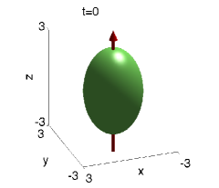
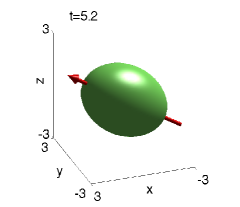
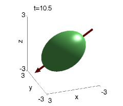
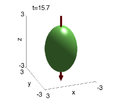
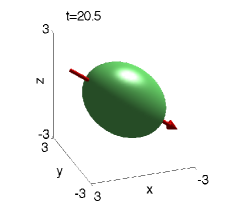
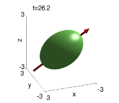
Figure 2: Isosurface plots of the density function $\rho(\mathbf{x},t)=|\psi(\mathbf{x},t)|^{2}=0.01$ and the dipole axis $\mathbf{n}(t)$ (red arrow) at different times for case 1 in the example 4.3.

  

  

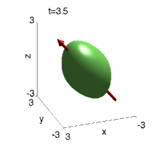
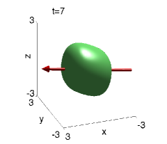
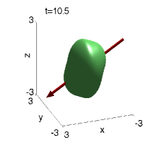
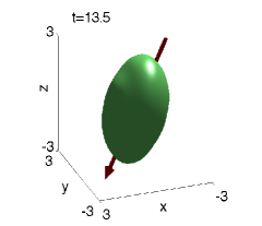
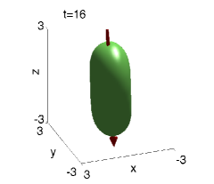
Figure 3: Isosurface plots of the density function $\rho(\mathbf{x},t)=|\psi(\mathbf{x},t)|^{2}=0.01$ and the dipole axis $\mathbf{n}(t)$ (red arrow) at different times for case 2 in the example 4.3.

Example 4.4.

Collapse and explosion of a dipolar BEC with damping effect in 3D.

In this case, the trapping potential $V(\mathbf{x})$ and the constants $\lambda$ and $\beta$ are set to be time dependent and are chosen according to the parameters used in the physical experiment [33, 32] (in dimensionless form) as follows:

$$V(\mathbf{x},t)=\left\{\begin{array}[]{ll}(\gamma_{x}^{2}x^{2}+\gamma_{y}^{2}y^{2}+\gamma_{z}^{2}z^{2})/2,&\quad t\in[0,\;4+t_{\rm hold}],\\[5.0pt] 0,&\quad{\rm otherwise,}\end{array}\right.$$ (4.57)

with $\gamma_{x}=1.65$, $\gamma_{y}=1$, $\gamma_{z}=1.325$,

$$\lambda(t)=\left\{\begin{array}[]{ll}82.864,&\quad t\in[0,\;5.6+t_{\rm hold}],\\[5.0pt] 0,&\quad{\rm otherwise},\end{array}\right.$$ (4.60)

$$\beta(t)=761.102\left\{\begin{array}[]{ll}1+\frac{28}{75t-280},&\quad t\in[0,\;3.2],\\[5.0pt] 0.3,&\quad t\in[3.2,\;3.6],\\[5.0pt] 1-\frac{1}{b(t-3.6)},&\quad t\in[3.6,\;4.8],\\[5.0pt] 38.8066,&\quad t\in[4.8,\;5.6+t_{\rm hold}],\\[5.0pt] 0,&\quad{\rm otherwise},\end{array}\right.$$ (4.66)

where

$$b(t)=\frac{1}{133}\left\{\begin{array}[]{ll}-125t-25e^{-5t}+215,&\quad t\in[0,\;0.4],\\[5.0pt] 25(1-e^{-2})e^{-6.25t+2.5}+140,&\quad t\in[0.4,\;1.2].\end{array}\right.$$ (4.69)

Here, $t_{\rm hold}$ is the hold time for the collapse, which is chosen as $t_{\rm hold}=0.2$. Moreover, we let $\mathbf{n}=(0,0,1)^{T}$, $\sigma=1$ and chose the damping term as $f(\rho)=\delta\rho^{2}$ with $\delta=3.512$, i.e., we chose the cubic nonlinearity and study the case of three-body loss of the particles. The initial data in (4.36) is chosen as $\psi_{0}(\mathbf{x})=\phi_{\rm gs}(\mathbf{x})$, where $\phi_{\rm gs}(\mathbf{x})$ is the ground state of the GPE (4.34) with $f(\rho)\equiv 0$, $\mathbf{n}=\mathbf{m}=\mathbf{n}(0)$, $\beta=\beta(0)$ $\lambda=\lambda(0)$ and $V(\mathbf{x})=V(\mathbf{x},0)$, which is computed numerically via the numerical method presented in the previous section. The computational domain and mesh size are chosen as $\mathcal{D}=[-24,24]^{3}$ and $h_{x}=h_{y}=h_{z}=\frac{3}{16}$, respectively. Figures 4 and 5 show the contour plot of the column density

$$\rho_{c}^{x}(y,z,t)=\int_{L_{x}}^{R_{x}}|\psi(\mathbf{x},t)|^{2}dx,$$

and the evolution of the total mass, respectively.

       

       

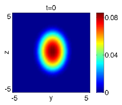
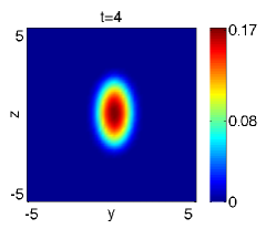
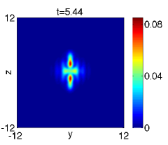
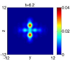
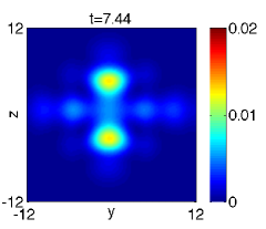
Figure 4: Contour plots of the column density $\rho_{c}^{x}(y,z,t)$ at different times for the example 4.4.

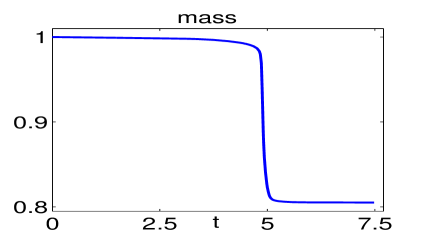
Figure 5: Evolution of the mass for the example 4.4.

From Figs. 4 and 5, we can conclude that: (i). The total mass is lost during the dynamics, especially during a very short period near $t=5$ (cf. Fig. 5). (ii). Although the BEC is released from the trap (i.e., the trapping potential is turned off) at time $t=4.2$, the atoms in the BEC still move inward in the $x$-$y$ plane. (iii). The density is first enlongated along the dipole orientation, then the collapse of the BEC happens very quickly, and “clover” pattern of the density profile is created. (iv). The “Leafs” are then ejected outward. All these results agree with those in the experiments [33, 32].

5 Conclusion

We proposed efficient and accurate numerical methods for computing the ground state and dynamics of the dipolar Bose-Einstein condensates by integrating a newly developed dipole-dipole interaction (DDI) solver via the non-uniform fast Fourier transform (NUFFT) algorithm [28] with existing numerical methods. The NUFFT based DDI solver removes naturally the singularity of the DDI at the origin by adopting the spherical/polar coordinates in the Fourier space, thus achieves spectral accuracy and simultaneously maintains high efficiency by appropriately combining the advantages of the NUFFT and FFT. Efficient and accurate numerical methods were then presented to compute the ground state and dynamics of the dipolar BEC with a DDI by integrating the normalized gradient flow with the backward Euler Fourier pseudospectral discretization and time-splitting Fourier pseudospectral method, respectively, together with NUFFT based DDI solver. Extensive numerical comparisons with existing methods were carried out to compute the DDI, ground states and dynamics of the dipolar BEC. Numerical results showed that our new methods outperformed other existing methods in terms of both accuracy and efficiency, especially when the computational domain is chosen smaller and/or the solution is anisotropic.

References

- [1] M. Abramowitz and I. A. Stegun, Handbook of Mathematical Functions, Dover, 1965.
- [2] K. Aikawa, A. Frisch, M. Mark, S. Baier, A. Rietzler, R. Grimm, F. Ferlaino, Bose-Einstein condensation of Erbium, Phys. Rev. Lett., 108 (2012), 210401.
- [3] J. O. Andersen, Theory of the weakly interacting Bose gas, Rev. Mod. Phys., 76 (2004), 599–639.
- [4] M. H. Anderson, J. R. Ensher, M. R. Matthewa, C. E. Wieman and E. A. Cornell, Observation of Bose-Einstein condensation in a dilute atomic vapor, Science, 269 (1995), 198–201.
- [5] X. Antoine, W. Bao and C. Besse, Computational methods for the dynamics of the nonlinear Schrodinger/Gross-Pitaevskii equations, Comput. Phys. Commun., 184 (2013), 2621-2633.
- [6] W. Bao, N. Ben Abdallah and Y. Cai, Gross-Pitaevskii-Poisson equations for dipolar Bose-Einstein condensate with anisotropic confinement, SIAM J. Math. Anal., 44 (2012), pp. 1713-1741.
- [7] W. Bao and Y. Cai, Mathematical theory and numerical methods for Bose-Einstein condensation, Kinet. Relat. Models, 6 (2013), pp. 1-135.
- [8] W. Bao, Y. Cai and H. Wang, Efficient numerical methods for computing ground states and dynamics of dipolar Bose-Einstein condensates, J. Comput. Phys., 229 (2010), pp. 7874–7892.
- [9] W. Bao, I-L. Chern and F. Lim, Efficient and spectrally accurate numerical methods for computing ground and first excited states in Bose-Einstein condensates, J. Comput. Phys., 219 (2006), 836–854.
- [10] W. Bao and Q. Du, Computing the ground state solution of Bose-Einstein condensates by a normalized gradient flow, SIAM J. Sci. Comput., 25 (2004), 1674–1697.
- [11] W. Bao and D. Jaksch, An explicit unconditionally stable numerical method for solving damped nonlinear Schrödinger equation with a focusing nonlinearity, SIAM J. Numer. Anal., 41 (2003), 1406–1426.
- [12] W. Bao, D. Jaksch and P. A. Markowich, Numerical solution of the Gross-Pitaevskii equation for Bose-Einstein condensation, J. Comput. Phys., 187 (2003), 318 - 342.
- [13] W. Bao, D. Jaksch and P. A. Markowich, Three dimensional simulation of jet formation in collapsing condensates, J. Phys. B: At. Mol. Opt. Phys., 37 (2004), 329–343.
- [14] W. Bao, D. Marahrens, Q. Tang and Y. Zhang, A simple and efficient numerical method for computing dynamics of rotating dipolar Bose–Einstein condensation via a rotating Lagrange coordinate, SIAM J. Sci. Comput., 35 (2013), A2671–A2695.
- [15] W. Bao, H. Jian, N. Mauser and Y. Zhang, Dimension reduction of the Schrödinger equation with Coulomb and anisotropic confining potentials, SIAM J. Appl. Math. 73 (6) (2013) 2100–2123.
- [16] W. Bao, S. Jiang, Q. Tang and Y. Zhang, Computing the ground state and dynamics of the nonlinear Schrödinger equation with nonlocal interactions via the nonuniform FFT, preprint, arXiv:1410.3584.
- [17] M. A. Baranov, Theoretical progress in many body physics of dipolar gases, Phys. Rep., 464 (2008), 71–111.
- [18] P. B. Blakie, C. Ticknor, A. S. Bradley, A. M. Martin, M. J. Davis, Y. Kawaguchi, Numerical method for evolving the dipolar projected Gross-Pitaevskii equation, Phys. Rev. E, 80 (2009), aritcle 016703.
- [19] I. Bloch, J. Dalibard and W. Zwerger, Many body physics with ultracold gases, Rev. Mod. Phys., 80 (2008), 885–965.
- [20] C. C. Bradley, C. A. Sackett, J. J. Tollett and R. G. Hulet, Evidence of Bose-Einstein condensation in an atomic gas with attractive interaction, Phys. Rev. Lett., 75 (1995), 1687–1690.
- [21] Y. Cai, M. Rosenkranz, Z. Lei and W. Bao, Mean-field regime of trapped dipolar Bose-Einstein condensates in one and two dimensions, Phys. Rev. A, 82 (2010), article 043623.
- [22] R. Carles, P. A. Markowich and C. Sparber, On the Gross-Pitaevskii equation for trapped dipolar quantum gases, Nonlinearity, 21 (2008), 2569–2590.
- [23] K. B. Davis, M. O. Mewes, M. R. Andrews, N. J. van Druten, D. S. Durfee, D. M. Kurn and W. Ketterle, Bose-Einstein condensation in a gas of sodium atoms, Phys. Rev. Lett., 75 (1995), 3969–3973.
- [24] A. L. Fetter, Rotating trapped Bose-Einstein condensates, Rev. Mod. Phys., 81 (2009), 647–691.
- [25] K. Góral, K. Rzayewski and T. Pfau, Bose–Einstein condensation with magnetic dipole-dipole forces, Phys. Rev. A, 61 (2000), article 051601(R).
- [26] A. Griesmaier, J. Werner, S. Hensler, J. Stuhler and T. Pfau, Bose–Einstein condensation of Chromium, Phys. Rev. Lett., 94 (2005), article 160401.
- [27] Z. Huang, P. A. Markowich and C. Sparber, Numerical simulation of trapped dipolar quantum gases: collapse studies and vortex dynamics, Kinetic and Related Models, 3 (2010), 181–194.
- [28] S. Jiang, L. Greengard and W. Bao, Fast and Accurate Evaluation of Nonlocal Coulomb and Dipole-Dipole Interactions via the Nonuniform FFT, SIAM J. Sci. Comput., 36 (2014), B777–B794.
- [29] T. F. Jiang, W. C. Su, Ground state of the dipolar Bose-Einstein condensate, Phys. Rev. A, 74 (2006), article 063602.
- [30] Y. Kawaguchi and M. Ueda, Spinor Bose-Einstein condensates, Phys. Rep., 520 (2012), 253–381.
- [31] T. Lahaye, T. Koch, B. Fröhlich, M. Fattori, J. Metz, A. Griesmaier, S. Giovanazzi, T. Pfau, Strong dipolar effects in a quantum ferrofluid, Nature, 448 (2007), 672–675.
- [32] T. Lahaye, C. Menotti, L. Santos, M. Lewenstein and T. Pfau, The physics of dipolar bosonic quantum gases, Rep. Prog. Phys., 72 (2009), 126401.
- [33] T. Lahaye, J. Metz, B. Fröhlich, T. Koch, M. Meister, A. Griesmaier, T. Pfau, H. Saito, Y. Kawaguchi, M. Ueda, D-wave collapse and explosion of a dipolar Bose-Einstein condensate, Phys. Rev. Lett., 101 (2008), article 080401.
- [34] A. J. Leggett, Bose-Einstein condensation in the alkali gases: Some fundamental concepts, Rev. Mod. Phys., 73 (2001), 307–356.
- [35] M. Lu, N. Q. Burdick, S. H. Youn and B. L. Lev, Strongly dipolar Bose–Einstein condensate of Dysprosium, Phys. Rev. Lett., 107 (2011), article 190401.
- [36] N. Mauser and Y. Zhang, Exact artificial boundary condition for the Poisson equation in the simulation of the 2D Schrödinger-Poisson system, Commun. Comput. Phys., 16 (3) (2014), 764–780.
- [37] O. Morsch and M. Oberthaler, Dynamics of Bose-Einstein condensates in optical lattices, Rev. Mod. Phys., 78 (2006), 179–215.
- [38] K.-K. Ni, S. Ospelkaus, M. H. G. de Miranda, A. Pe’er, B. Neyenhuis, J. J. Zirbel, S. Kotochigova, P. S. Julienne, D. S. Jin, J. Ye, A high phase-space-density gas of polar molecules, Science, 322 (2008), 231–235.
- [39] D. H. J. O’Dell, S. Giovanazzi and C. Eberlein, Exact hydrodynamics of a trapped dipolar Bose-Einstein condensate, Phys. Rev. Lett., 92 (2004), article 250401.
- [40] N. G. Parker, C. Ticknor, A. M. Martin, D. H. J. O’Dell, Structure formation during the collapse of a dipolar atomic Bose-Einstein condensate, Phys. Rev. A, 79 (2009), article 013617.
- [41] L. P. Pitaevskii and S. Stringari, “Bose-Einstein Condensation”, Clarendon Press, Oxford, 2003.
- [42] S. E.Pollack, D. Dries, M. Junker, Y. P. Chen, T. A. Corcovilos, R. G. Hulet, Extreme tunability of interactions in a Bose-Einstein condensate, Phys. Rev. Lett., 102 (2009), 090402.
- [43] L. Santos, G. Shlyapnikov, P. Zoller, M. Lewenstein, Bose-Einstein condensation in trapped dipolar gases, Phys. Rev. Lett., 85 (2000), 1791–1797.
- [44] E. S. Shuman, J. F. Barry, D. Demille, Laser cooling of a diatomic molecule, Nature, 467 (2010), 820–823.
- [45] G. Strang, On the construction and comparision of difference schemes, SIAM J. Numer. Anal., 5 (1968), 505-517.
- [46] C. Ticknor, N.G. Parker, A. Melatos, S.L. Cornish, D.H.J. O’Dell, A.M. Martin, Collapse times of dipolar Bose-Einstein condensates, Phys. Rev. A, 78 (2008), article 061607.
- [47] M. Vengalattore, S. R. Leslie, J. Guzman, D. M. Stamper-Kurn, Spontaneously modulated spin textures in a dipolar spinor Bose-Einstein condensate, Phys. Rev. Lett., 100 (2008), 170403.
- [48] S. Yi, L. You, Trapped condensates of atoms with dipole interactions, Phys. Rev. A, 63 (2001), article 053607.
- [49] Y. Zhang and X. Dong, On the computation of ground state and dynamics of Schrödinger-Poisson-Slater system, J. Comput. Phys., 230 (2011), 2660–2676.