Pricing and Risk Management
with High-Dimensional Quasi Monte Carlo
and Global Sensitivity Analysis

Abstract

We review and apply Quasi Monte Carlo (QMC) and Global Sensitivity Analysis (GSA) techniques to pricing and risk management (greeks) of representative financial instruments of increasing complexity. We compare QMC vs standard Monte Carlo (MC) results in great detail, using high-dimensional Sobol’ low discrepancy sequences, different discretization methods, and specific analyses of convergence, performance, speed up, stability, and error optimisation for finite differences greeks. We find that our QMC outperforms MC in most cases, including the highest-dimensional simulations and greeks calculations, showing faster and more stable convergence to exact or almost exact results. Using GSA, we are able to fully explain our findings in terms of reduced effective dimension of our QMC simulation, allowed in most cases, but not always, by Brownian bridge discretization. We conclude that, beyond pricing, QMC is a very promising technique also for computing risk figures, greeks in particular, as it allows to reduce the computational effort of high-dimensional Monte Carlo simulations typical of modern risk management.

JEL classifications: C63, G12, G13.

Keywords: derivative, option, European, Asian, barrier, knock-out, cliquet, greeks, Brownian bridge, global sensitivity analysis, Monte Carlo, Quasi Monte Carlo, random, pseudo random, quasi random, low discrepancy, Sobol’, convergence, speed-up

Acknowledgements: M.B. acknowledges fruitful discussions with many colleagues at international conferences, in Risk Management of Intesa Sanpaolo, and in Financial Engineering and Trading Desks of Banca IMI.

Disclaimer: the views expressed here are those of the authors and do not represent the opinions of their employers. They are not responsible for any use that may be made of these contents.

1 Introduction

Nowadays market and counterparty risk measures, based on multi-dimensional, multi-step Monte Carlo simulations, are very important tools for managing risk, both on the front office side, for sensitivities (greeks) and credit, funding, capital valuation adjustments (CVA, FVA, KVA, generically called XVAs) and on the risk management side, for risk measures and capital allocation. Furthermore, they are typically required for regulatory risk internal models and validated by regulators. The daily production of prices and risk measures for large portfolios with multiple counterparties is a computationally intensive task, which requires a complex framework and an industrial approach. It is a typical high budget, high effort project in banks.

In the past decades, much effort was devoted to the application of Monte Carlo techniques to derivatives pricing [Boy77, BBG97, Jac01, Gla03]. The main reason is that complex financial instruments usually cannot be priced through analytical formulas, and the computation of high-dimensional integrals is required. Monte Carlo simulation is, then, a common way to tackle such problems, since it reduces integration to function evaluations at many random points and to averaging on such values. As a result, virtually any product can be easily priced in any dimension. However, this method is rather time consuming and the convergence rate is slow, since the root mean square error decays as $N^{-1/2}$, where $N$ is the number of sampled points. Various “variance reduction” techniques exist, which can improve the efficiency of the simulation, but they don’t modify the convergence rate [Jac01, Gla03].

Quasi Monte Carlo represents a very efficient alternative to standard Monte Carlo, capable to achieve, in many cases, a faster convergence rate and, hence, higher accuracy [Jac01, Gla03, MF99, SK05b, SK05a, Wan09, KFSM11, SAKK12]. The idea behind Quasi Monte Carlo methods is to use, instead of pseudo-random numbers (PRN), low discrepancy sequences (LDS, also known as quasi-random numbers) for sampling points. Such LDS are designed in such a way that the integration domain is covered as uniformly as possible, while PRN are known to form clusters of points and always leave some empty areas. Indeed, the very random nature of PRN generators implies that there is a chance that newly added points end up near to previously sampled ones, thus they are wasted in already probed regions which results in rather low convergence. On the contrary, LDS “know” about the positions of previously sampled points and fill the gaps between them. Among several known LDS, Sobol’ sequences have been proven to show better perfomance than others and for this reason they are widely used in Finance [Jac01, Gla03]. However, it is also known that construction of efficient Sobol’ sequences heavily depends on the so-called initial numbers and therefore very few Sobol’ sequence generators show good efficiency in practical tests [SAKK12].

Compared to Monte Carlo, Quasi Monte Carlo techniques also have some disadvantages. Firstly, there is no “in sample” estimation of errors: since LDS are deterministic, there is not a notion of probabilistic error. There have been developed some techniques, known under the name of randomized Quasi Monte Carlo, which introduce appropriate randomizations in the construction of LDS, opening up the possibility of measuring errors through a confidence interval while preserving the convergence rate of Quasi Monte Carlo [Gla03]. The drawback is the sacrifice of computational speed and, often, of some precision. Secondly, effectiveness of Quasi Monte Carlo depends on the integrand function, and, most importantly, the convergence rate can depend on the dimensionality of the problem. The latter can be seen as a big obstacle, since many problems in financial engineering (especially in risk management) are known to be high-dimensional. However, many financial applications have been reported where Quasi Monte Carlo outperforms standard Monte Carlo even in the presence of very high dimensions [PT95, PP99, CMO97, KMRZ98a, KMRZ98b, KS07, SAKK12]. This fact is usually explained by a reduced effective dimension of the problem, with respect to its nominal dimension. The concept of effective dimensions was introduced in [CMO97]. It was suggested that QMC is superior to MC if the effective dimension of an integrand is not too large. The notion is based on the ANalysis Of VAriances (ANOVA). In [LO00] it was shown how the ANOVA components are linked to the effectiveness of QMC integration methods. It is important to measure the effective dimension in order to predict the efficiency of a Quasi Monte Carlo algorithm. Moreover, various techniques can be used to reduce effective dimension and, thus, improve efficiency: this is possible because the effective dimension can vary by changing the order in which the variables are sampled. The optimal way to achieve this can be a hard task, it could depend on the specific model and a general solution is not known at present. One popular choice in the financial literature on path-dependent option pricing [CMO97, KS07] is to apply the Brownian bridge discretization to the simulation of the underlying stochastic process, which is based on the use of conditional distributions. Unlike the standard discretization, which generates values of the Brownian motion sequentially along the time horizon, the Brownian bridge discretization first generates the Brownian motion value at the terminal point, then it fills a midpoint using the value already found at the terminal point and then subsequent values at the successive midpoints using points already simulated at previous steps. In terms of QMC sampling, this simulation scheme means that the first coordinate of the QMC vector is used to simulate the terminal value of the Brownian motion, while subsequent coordinates are used to generate intermediate points. There are many studies which show that superior performance of the QMC approach with the Brownian bridge discretization in comparison with the standard discretization using MC or QMC sampling, in application e.g. to Asian options [CMO97, KS07]. However, it was pointed in [Pap01] that, in some cases, the Brownian bridge can perform worse than the standard discretization in QMC simulation. The big question is how to know with certainty which numerical scheme will provide superior efficiency in QMC simulation. Global Sensitivity Analysis (GSA) is the answer.

GSA is a very powerful tool in the analysis of complex models as it offers a comprehensive approach to model analysis. Traditional sensitivity analysis, called local within the present context, applied to a function $f(x)$ is based on specifying a point $x_{0}$ in the function domain and then computing a derivative $\frac{\partial f}{\partial x}$ at $x=x_{0}$. GSA instead does not require to specify a particular point $x_{0}$ in the domain, since it explores the whole domain (hence the name global). It also quantifies the effect of varying a given input (or set of inputs) while all other inputs are varied as well, providing a measure of interactions among variables. GSA is used to identify key parameters whose uncertainty most affects the output. This information can be used to rank variables, fix unessential variables and decrease problem dimensionality. Reviews of GSA can be found in [SK05a] and [SAA⁺10]. The variance-based method of global sensitivity indices developed by Sobol’ [Sob01] became very popular among practitioners due to its efficiency and easiness of interpretation. There are two types of Sobol’ sensitivity indices: the main effect indices, which estimate the individual contribution of each input parameter to the output variance, and the total sensitivity indices, which measure the total contribution of a single input factor or a group of inputs.

For modelling and complexity reduction purposes, it is important to distinguish between the model nominal dimension and its effective dimension. The notions of effective dimension in the truncation and superposition sense were introduced in [CMO97]. Further, Owen added the notion of “average dimension” which is more practical from the computational point of view [LO06]. Definitions and evaluations of effective dimensions are based on the knowledge of Sobol’ sensitivity indices. Quite often complex mathematical models have effective dimensions much lower than their nominal dimensions. The knowledge of model effective dimensions is very important since it allows to apply various complexity reduction techniques. In the context of quantitative Finance, GSA can be used to estimate effective dimensions of a given problem. In particular, it can assess the efficiency of a particular numerical scheme (such as the Brownian bridge or standard discretizations).

The paper is organized as follows: Section 2 contains a brief review on Quasi Monte Carlo methodology and on Low Discrepancy Sequences, with particular emphasis on financial applications. Section 3 introduces GSA and the notions of effective dimensions, establishing a link with QMC efficiency. In Section 4 we present the results of prices and sensitivities (greeks) computation for selected payoffs: both GSA and convergence analysis are performed, with the purpose to compare MC and QMC efficiencies via a thorough error analysis. Finally, conclusions and directions of future work are given in Section 5. In particular we propose to apply our methodology to risk management issues, where a faster and smoother convergence would represent a great advantage in terms of both computational effort and budget. Some technical details are discussed in the Appendices.

2 Monte Carlo and Quasi Monte Carlo Methods in Finance

2.1 General motivation

In Finance, many quantities of interest, such as prices and greeks, are defined as expectation values under a given probability measure, so their evaluation requires the computation of multidimensional integrals of a (generally complicated) function.

Let’s consider a generic financial instrument written on a single asset $S$ with a single payment date $T$. We denote the instrument’s payoff at time $T$ as $\mathcal{P}(S_{t},\bm{\theta})$, where $S_{t}$ is the underlying asset value at time $t\in[0,T]$, and $\bm{\theta}$ is a set of relevant parameters, including instrument parameters, such as strikes, barriers, fixing dates of the underlying $S$, callable dates, payment dates, etc., described in the contract, and pricing parameters, such as interest rates, volatilities, correlations, etc., associated with the pricing model.

Using standard no-arbitrage pricing theory, see e.g. [Duf01], the price of the instrument at time $t=0$ is given by

$$V_{0}(\bm{\theta})=\mathbb{E}^{Q}[D(0,T)\mathcal{P}(S_{t},\bm{\theta})|\mathcal{F}_{0}],$$ (2.1)

$$D(0,T)=\exp{\left(-\int_{0}^{T}r(t)dt\right)},$$ (2.2)

where $\left(\Omega,\mathcal{F},Q\right)$ is a probability space with risk-neutral probability measure $Q$ and filtration $\mathcal{F}_{t}$ at time $t$, $\mathbb{E}^{Q}[\,\cdot\,]$ is the expectation with respect to $Q$, $D(0,T)$ is the stochastic discount factor, and $r(t)$ is the risk-neutral short spot interest rate. Notice that the values of $S$ at intermediate times $t$ before final payment date $T$ may enter into the definition of the payoff $\mathcal{P}$.

In order to price the financial instrument, we assume a generic Wiener diffusion model for the dynamics of the underlying asset $S$,

$$dS_{t}=\mu\left(t,S_{t}\right)dt+\sigma\left(t,S_{t}\right)dW^{P}_{t},$$ (2.3)

with initial condition $S_{0}$, where $P$ is the real-world probability measure, $\mu$ is the real-world drift, $\sigma$ is the volatility, and $W^{P}_{t}$ is a Brownian motion under $P$, such that $dW_{t}\sim Z\sqrt{dt}$, where $Z\sim N(0,1)$ is a standard normal random variable. The solution to eq. (2.3) is given by

$$S_{t}=S_{0}+\int_{0}^{t}\mu\left(u,S_{u}\right)du+\int_{0}^{t}\sigma\left(u,S_{u}\right)dW^{P}_{u}\,,$$ (2.4)

see e.g. [Oks92]. In particular, in the Black-Scholes model the underlying asset $S_{t}$ follows a simple log-normal stochastic process

$$dS_{t}=\mu\,S_{t}\,dt+\sigma\,S_{t}\,dW^{P}_{t},$$ (2.5)

with constant $\mu$ and $\sigma$. The solution to equation (2.5) in a risk-neutral world (under the risk-neutral probability measure $Q$) is given by

$$S_{t}=S_{0}\exp{\left[\left(r-\frac{1}{2}\sigma^{2}\right)t+\sigma W^{Q}_{t}\right]}.$$ (2.6)

“Greeks” are derivatives of the price $V_{0}(\bm{\theta})$ w.r.t. specific parameters $\bm{\theta}$. They are very important quantities which need to be computed for hedging and risk management purposes. In the present work, we will consider in particular the following greeks:

$$\Delta =\frac{\partial V_{0}}{\partial S_{0}},$$ (2.7)

$$\Gamma =\frac{\partial^{2}V_{0}}{\partial S^{2}_{0}},$$ (2.8)

$$\mathcal{V} =\frac{\partial V_{0}}{\partial\sigma},$$ (2.9)

called delta, gamma and vega, respectively. Notice that, in the Black-Scholes model, delta is exactly the hedge of the financial instrument w.r.t. the risky underlying $S$, and vega is a derivative w.r.t. a model parameter (the constant volatility $\sigma$ in the Black-Scholes SDE (2.5)).

The solution to the pricing equation (2.1) requires the knowledge of the values of the underlying asset $S$ at the relevant contract dates $\left\{T_{1},\ldots,T_{n}\right\}$. Such values may be obtained by solving the SDE (2.4). If the SDE cannot be solved explicitly, we must resort to a discretization scheme, computing the values of $S$ on a time grid $\left\{t_{1},\ldots,t_{D}\right\}$, where $t_{1}<t_{2}<\cdots<t_{D}$, and $D$ is the number of time steps. Notice that the contract dates must be included in the time grid, $\left\{T_{1},\ldots,T_{n}\right\}\subset\left\{t_{1},\ldots,t_{D}\right\}$. For example, the Euler discretization scheme consists of approximating the integral equation (2.4) by

$$S_{j}=S_{j-1}+\mu\left(t_{j-1},S_{j-1}\right)\Delta t_{j}+\sigma\left(t_{j-1},S_{j-1}\right)\Delta W_{j},\quad j=1,\ldots,D,$$ (2.10)

where $\Delta t_{j}=t_{j}-t_{j-1}$, $\Delta W_{j}=W_{j}-W_{j-1}$, and $t_{0}=0$. In particular, the discretization of the Black-Scholes solution (2.6) leads to

$$S_{j}=S_{j-1}\exp{\left[\left(r-\frac{\sigma^{2}}{2}\right)\Delta t_{j}+\sigma\Delta W_{j}\right]},\quad j=1,\ldots,D.$$ (2.11)

Clearly, the price in eq. (2.1) will depend on the discretization scheme adopted. See [KP95] for the order of convergence of Euler and other discretization schemes.

We consider two discretization schemes in eq. (2.11): standard discretization (SD) and Brownian bridge discretization (BBD). In the SD scheme the Brownian motion is discretized as follows:

$$\Delta W_{j}=\sqrt{\Delta t_{j}}Z_{j},\quad j=1,\ldots,D.$$ (2.12)

In the BBD scheme the first variate is used to generate the terminal value of the Brownian motion, while subsequent variates are used to generate intermediate points, conditioned to points already simulated at earlier and later time steps, according to the following formula,

$$\begin{split}&W_{0}=0,\\ &W_{D}=\sqrt{\Delta t_{D0}}Z_{1},\\ &W_{j}=\frac{\Delta t_{kj}}{\Delta t_{ki}}\,W_{i}+\frac{\Delta t_{ji}}{\Delta t_{ki}}\,W_{k}+\sqrt{\frac{\Delta t_{kj}\Delta t_{ji}}{\Delta t_{ki}}}Z_{l},\quad t_{i}<t_{j}<t_{k}\,,\;\;\;l=2,\ldots,D,\end{split}$$ (2.13)

where $\Delta t_{ab}=t_{a}-t_{b}$. Unlike the SD scheme, which generates the Brownian motion sequentially across time steps, the BBD scheme uses different orderings: as a result, the variance in the stochastic part of (2.13) is smaller than that in (2.12) for the same time steps, so that the first few points contain most of the variance. Both schemes have the same variance, hence their MC convergence rates are the same, but QMC sampling shows different efficiencies for SD and BBD, which will be discussed in the following sections.

The number $D$ of time steps required in the discretization of the SDE (2.10) is the nominal dimension of the computational problem: indeed, the expectation value in (2.1) is formally an integral of the payoff, regarded as a function of $Z_{1},\ldots,Z_{D}$. In general, financial instruments may depend on multiple underlying assets $S^{1},\ldots,S^{M}$: in this case, the dimension of the problem is given by $D\times M$. In conclusion, the pricing problem (2.1) is reduced to the evaluation of high-dimensional integrals. This motivates the use of Monte Carlo techniques.

Throughout this work, we will focus on the relative effects of the dimension $D$ and of the discretization schemes on the MC and QMC simulations. Thus, we will assume a simple Black-Scholes underlying dynamics for simplicity. This choice will be also useful as a reference case to interpret further results based on more complex dynamics. We stress that using simple and solvable dynamics is an approximation often used in risk management practice for risk measures calculation on large portfolios with multiple underlying risk factors, because of computational bottlenecks.

2.2 Pseudo Random Numbers and Low Discrepancy Sequences

Standard gaussian numbers ${Z_{j}}$ are computed using transformation of uniform variates $x_{j}\sim\ i.i.d.\;U(0,1)$,

$$Z_{j}=\Phi^{-1}(x_{j}),\quad j=1,\ldots,D,$$ (2.14)

where $\Phi^{-1}$ is the inverse cumulative distribution function of the standard normal distribution. Hence the pricing problem (2.1) can be reduced to the evaluation of integrals of the following generic form

$$V=\int_{H^{D}}f(\bm{x})d^{D}\bm{x},$$ (2.15)

where $H^{D}=[0,1]^{D}$ is the $D-$dimensional unit hypercube. The standard Monte Carlo estimator of (2.15) has the form

$$V_{N}\simeq\frac{1}{N}\sum_{k=1}^{N}f(\bm{x}_{k}),$$ (2.16)

where $\left\{\bm{x}_{k}\right\}_{k=1}^{N}$ is a sequence of $N$ random points in $H^{D}$. Sequences $\left\{\bm{x}_{k}\right\}_{k=1}^{N}$ are produced by appropriate Random Number Generators (RNGs). In particular, Pseudo Random Number Generators (PRNGs) are computer algorithms that produce deterministic sequences of pseudo random numbers (PRNs) mimicking the properties of true random sequences. Such sequences are completely determined by a set of initial values, called the PRNG’s state. Thus, pseudo random sequences are reproducible, using the same set of state variables. PRNGs are characterized by the seed, i.e. a random number used to initialize the PRNG, the period, i.e. the maximum length, over all possible state variables, of the sequence without repetition, and the distribution of the generated random numbers, which is generally uniform $[0,1)$. The most famous PRNG is the Mersenne Twister [MN98], with the longest period of $2^{19937}-1$ and good equidistribution properties guaranteed up to, at least, 623 dimensions. Pseudo random sequences are known to be plagued by clustering: since new points are added randomly, they don’t necessarily fill the gaps among previously sampled points. This fact causes a rather slow convergence rate. Consider an integration error

$$\varepsilon=|V-V_{N}|.$$ (2.17)

By the Central Limit Theorem the root mean square error of the Monte Carlo method is

$$\varepsilon_{MC}=\left[\mathbb{E}(\varepsilon^{2})\right]^{1/2}=\frac{\sigma_{f}}{\sqrt{N}}\,,$$ (2.18)

where $\sigma_{f}$ is the standard deviation of $f(x)$. Although $\varepsilon_{MC}$ does not depend on the dimension $D$, as in the case of lattice integration on a regular grid, it decreases slowly with increasing $N$. Variance reduction techniques, such as antithetic variables [Jac01, Gla03], only affect the numerator in (2.18).

In order to increase the rate of convergence, that is to increase the power of $N$ in the denominator of (2.18), one has to resort to Low Discrepancy Sequences (LDS), also called Quasi Random Numbers (QRNs), instead of PRNs. The discrepancy of a sequence $\left\{\bm{x}_{k}\right\}_{k=1}^{N}$ is a measure of how inhomogeneously the sequence is distributed inside the unit hypercube $H^{D}$. Formally, it is defined by [Jac01]

$$\begin{split}&\mathcal{D}^{D}_{N}(\bm{x}_{1},\ldots,\bm{x}_{N})=\underset{\bm{\xi}\in H^{D}}{\sup}\left|\frac{n\left[\mathcal{S}^{D}(\bm{\xi}),\bm{x}_{1},\ldots,\bm{x}_{N}\right]}{N}-m(\bm{\xi})\right|,\\ &\mathcal{S}^{D}(\bm{\xi})=[0,\xi_{1})\times\cdots\times[0,\xi_{D})\subset H^{D},\quad m(\bm{\xi})=\prod_{j=1}^{D}\xi_{j},\\ \end{split}$$ (2.19)

where

$$\begin{split}&n\left[\mathcal{S}^{D}(\bm{\xi}),\bm{x}_{1},\ldots,\bm{x}_{N}\right]=\sum_{k=1}^{N}\mathds{1}_{\left\{\bm{x}_{k}\in\mathcal{S}^{D}(\bm{\xi})\right\}}=\sum_{k=1}^{N}\prod_{j=1}^{D}\mathds{1}_{\left\{x_{k,j}\leq\xi_{j}\right\}}\,\end{split}$$ (2.20)

is the number of sampled points that are contained in hyper-rectangle $\mathcal{S}^{D}\subset H^{D}$. It can be shown that the expected discrepancy of a pseudo random sequence is of the order of $\ln(\ln N)/\sqrt{N}$. A Low Discrepancy Sequence is a sequence $\left\{\bm{x}_{k}\right\}_{k=1}^{N}$ in $H^{D}$ such that, for any $N>1$, the first $N$ points ${\bm{x}_{1},\ldots,\bm{x}_{N}}$ satisfy inequality

$$\mathcal{D}^{D}_{N}(\bm{x}_{1},\ldots,\bm{x}_{N})\leq c(D)\frac{\ln^{D}N}{N}\,,$$ (2.21)

for some constant $c(D)$ depending only on $D$ [Nie88]. Unlike PRNGs, Low Discrepancy Sequences are deterministic sets of points. They are typically constructed using number theoretical methods. They are designed to cover the unit hypercube as uniformly as possible. In the case of sequential sampling, new points take into account the positions of already sampled points and fill the gaps between them. Notice that a regular grid of points in $H^{D}$ does not ensure low discrepancy, since projecting adjacent dimensions easily produces overlapping points.

A Quasi Monte Carlo (QMC) estimator of the integral (2.15) is of the form (2.16) with the only difference that the sequence $\left\{\bm{x}_{k}\right\}_{k=1}^{N}$ is sampled using LDS instead of PRNs. An upper bound for the QMC integration error is given by the Koksma-Hlawka inequality

$$\varepsilon_{QMC}\leq V(f)\mathcal{D}^{D}_{N}=\mathcal{O}\left(\frac{\ln^{D}N}{N}\right)\,,$$ (2.22)

where $V(f)$ is the variation of the integrand function in the sense of Hardy and Krause, which is finite for functions of bounded variation [KFSM11]. The convergence rate of (2.22) is asymptotically faster than (2.18), but it is rather slow for feasible $N$. Moreover, it depends on the dimensionality $D$. However, eq. (2.22) is just an upper bound: what is observed in most numerical tests [KFSM11, CMO97] is a power law

$$\varepsilon_{QMC}\sim\frac{c}{N^{\alpha}}\,,$$ (2.23)

where the value of $\alpha$ depends on the model function and, therefore, is not a priori determined as for MC. When $\alpha>0.5$ the QMC method outperforms standard MC: this situation turns out to be quite common in financial problems. We will measure $\alpha$ for some representative financial instruments, showing that its value can be very close to 1 when the effective dimension of $f$ is low, irrespective of the nominal dimension $D$. The concept of effective dimension, and the methodology to compute it, will be introduced in the following sections.

We stress that, since LDS are deterministic, there are no statistical measures like variances associated with them. Hence, the constant $c$ in (2.23) is not a variance and (2.23) does not have a probabilistic interpretation as for standard MC. To overcome this limitation, Owen suggested to introduce randomization into LDS at the same time preserving their superiority to PRN uniformity properties [Owe93]. Such LDS became known as scrambled (see also [Gla03]). In practice, the integration error for both MC and QMC methods for any fixed $N$ can be estimated by computing the following error averaged over $L$ independent runs:

$$\varepsilon_{N}=\sqrt{\frac{1}{L}\,\sum_{\ell=1}^{L}\left(V-V_{N}^{(\ell)}\right)^{2}},$$ (2.24)

where $V$ is the exact, or estimated at a very large extreme value of $N\rightarrow\infty$, value of the integral and $V_{N}^{(\ell)}$ is the simulated value for the $\ell$th run, performed using $N$ PRNs, LDS, or scrambled LDS. For MC and QMC based on scrambled LDS, runs based on different seed points are statistically independent. In the case of QMC, different runs are obtained using non overlapping sections of the LDS. Actually, scrambling LDSs weakens the smoothness and stability properties of the Monte Carlo convergence, as we will see in Section 4.5. Hence, in this paper we will use the approach based on non-overlapping LDSs, as in [SK05b].

The most known LDS are Halton, Faure, Niederreiter and Sobol’ sequences. Sobol’ sequences, also called $LP\tau$ sequences or $(t,s)$ sequences in base 2 [Nie88], became the most known and widely used LDS in finance due to their efficiency [Jac01, Gla03]. Sobol’ sequences were constructed under the following requirements [Sob67]:

1. Best uniformity of distribution as $N\to\infty$.

2. Good distribution for fairly small initial sets.

3. A very fast computational algorithm.

The efficiency of Sobol’ LDS depend on the so-called initialisation numbers. In this work we used SobolSeq8192 generator provided by BRODA [BRO]. SobolSeq is an implementation of the 8192 dimensional Sobol’ sequences with modified initialisation numbers. Sobol’ sequences produced by SobolSeq8192 can be up to and including dimension $2^{13}$, and satisfy additional uniformity properties: Property A for all dimensions and Property A’ for adjacent dimensions (see [SAKK12] for details). It has been found in [SAKK12] that SobolSeq generator outperforms all other known LDS generators both in speed and accuracy.

3 Global Sensitivity Analysis and Effective Dimensions

As we mentioned in the Introduction and Section 2.2, effective dimension is the key to explain the superior efficiency of QMC w.r.t. MC. Hence, it is crucial to develop techniques to estimate the effective dimension and to find the most important variables in a MC simulation.

The variance-based method of global sensitivity indices developed by Sobol’ became very popular among practitioners due to its efficiency and easiness of interpretation [SK05a, SAA⁺10]. There are two types of Sobol’ sensitivity indices: the main effect indices, which estimate the individual contribution of each input parameter to the output variance, and the total sensitivity indices, which measure the total contribution of a single input factor or a group of inputs. Sobol’ indices can be used to rank variables in order of importance, to identify non-important variables, which can then be fixed at their nominal values to reduce model complexity, and to analyze the efficiency of various numerical schemes.

Consider a mathematical model described by an integrable function $f(x)$, where the input $x=(x_{1},\ldots,x_{D})$ is taken in a $D$-dimensional domain $\Omega$ and the output is a scalar. Without loss of generality, we choose $\Omega$ to be the unit hypercube $H^{D}$. The input variables $x_{1},\ldots,x_{D}$ can, then, be regarded as independent uniform random variables each defined in the unit interval $[0,1]$. The starting point of global sensitivity analysis (GSA) is the analysis of variance (ANOVA) decomposition of the model function,

$$f(x)=f_{0}+\sum_{i}f_{i}(x_{i})+\sum_{i<j}f_{ij}(x_{i},x_{j})+\ldots+f_{1\,2\cdots D}(x_{1},\ldots,x_{D})\,.$$ (3.1)

The expansion (3.1) is unique, provided that

$$\int_{0}^{1}f_{i_{1}\cdots i_{s}}(x_{i_{1}},\ldots,x_{i_{s}})dx_{i_{k}}=0\,,\;\;\;\forall k=1,\ldots,s\,.$$ (3.2)

The ANOVA decomposition expands the function $f$ into a sum of terms, each depending on an increasing number of variables: a generic component $f_{i_{1}\cdots i_{s}}(x_{i_{1}},\ldots,x_{i_{s}})$, depending on $s$ variables, is called an $s$-order term. It follows from (3.2) that the ANOVA decomposition is orthogonal and that its terms can be explicitly found as follows,

$$\begin{split}f_{0}=&\int_{H^{D}}f(x)d^{D}x,\\ f_{i}(x_{i})=&\int_{H^{D-1}}f(x)\prod_{k\neq i}dx_{k}\,-f_{0},\\ f_{ij}(x_{i},x_{j})=&\int_{H^{D-2}}f(x)\prod_{k\neq i,j}dx_{k}\,-f_{0}-f_{i}(x_{i})-f_{j}(x_{j}),\end{split}$$ (3.3)

and so on. If $f$ is square-integrable, its variance decomposes into a sum of partial variances:

$$\sigma^{2}=\sum_{i}\sigma^{2}_{i}+\sum_{i<j}\sigma^{2}_{ij}+\ldots+\sigma^{2}_{12\cdots D},$$ (3.4)

where

$$\sigma^{2}_{i_{1}\cdots i_{s}}=\int_{0}^{1}f^{2}_{i_{1}\cdots i_{s}}(x_{i_{1}},\ldots,x_{i_{s}})dx_{i_{1}}\cdots dx_{i_{s}}.$$ (3.5)

Sobol’ sensitivity indices are defined as

$$S_{i_{1}\cdots i_{s}}=\frac{\sigma^{2}_{i_{1}\cdots i_{s}}}{\sigma^{2}}$$ (3.6)

and measure the fraction of total variance accounted by each $f_{i_{1}\cdots i_{s}}$ term of the ANOVA decomposition. From (3.4) it follows that all Sobol’ indices are non negative and normalized to 1. First order Sobol’ indices $S_{i}$ measure the effect of single variables $x_{i}$ on the output function; second order Sobol’ indices $S_{ij}$ measure the interactions between pairs of variables, i.e. the fraction of total variance due to variables $x_{i}$ and $x_{j}$ which cannot be explained by a sum of effects of single variables; higher order Sobol’ indices $S_{i_{1}\cdots i_{s}}$, with $s>2$, measure the interactions among multiple variables, i.e. the fraction of total variance due to variables $x_{i_{1}},\ldots,x_{i_{s}}$ which cannot be explained by a sum of effects of single variables or lower order interactions.

The calculation of Sobol’ sensitivity indices in eq. (3.6) requires, in principle, $2^{D}$ valuations of the multi-dimensional integrals in eq. (3.5), which is a very cumbersome, or even impossible, computational task. Furthermore, for practical purposes, and in particular when the function $f$ has low order interactions, it is not actually necessary to know all the possible Sobol’ indices, but just an appropriate selection of them. Thus, it is very useful to introduce Sobol’ indices for subsets of variables and total Sobol’ indices. Let $y=\left\{x_{i_{1}},\ldots,x_{i_{m}}\right\}\subseteq x,1\leq i_{1}\leq\ldots,\leq i_{m}\leq D$, be a subset of $x$, and $z=y^{\complement}\subseteq x$ its complementary subset, and define

$$\begin{split}&S_{y}=\sum_{s=1}^{D}\,\sum_{(i_{1}<\cdots<i_{s})\in K}S_{i_{1}\cdots i_{s}},\\ &S_{y}^{tot}=\,1-S_{z}\,,\end{split}$$ (3.7)

where $K=\{i_{1},\ldots,i_{m}\}$. Notice that $0\leq S_{y}\leq S_{y}^{tot}\leq 1$. The quantity $S_{y}^{tot}-S_{y}$ accounts for all the interactions between the variables in subsets $y$ and $z$. It turns out that there exist efficient formulas which allow to avoid the knowledge of ANOVA components and to compute Sobol’ indices directly from the values of function $f$ [Sob01]. These formulas are based on the following integrals,

$$\begin{split}S_{y}=&\frac{1}{\sigma^{2}}\,\int_{0}^{1}[f(y^{\prime},z^{\prime})-f_{0}][f(y^{\prime},z)-f(y,z)]dy\,dz\,dy^{\prime}dz^{\prime}\,,\\ S_{y}^{tot}=&\frac{1}{2\sigma^{2}}\,\int_{0}^{1}[f(y,z)-f(y^{\prime},z)]^{2}dy\,dz\,dy^{\prime}\,,\\ \sigma^{2}=&\int_{0}^{1}f^{2}(y,z)dy\,dz\,-f_{0}^{2}\,,\\ f_{0}=&\int_{0}^{1}f(y,z)dy\,dz\,,\end{split}$$ (3.8)

where the integration variables are the components of the vectors $y,z,y^{\prime},z^{\prime}$, such that $x=y\cup z$, and the first two integrals depend on the choice of $y$. Such integrals can be evaluated, in general, via MC/QMC techniques [KFSM11, Sal02].

Furthermore, usually enough information is already given by the first order indices $S_{i}$ and by corresponding total effect indices $S_{i}^{tot}$, linked to a single variable $y=\left\{x_{i}\right\}$. For these Sobol’ indices, it’s easy to see that

• $S_{i}^{tot}=0$: the output function does not depend on $x_{i}$,

• $S_{i}=1$: the output function depends only on $x_{i}$,

• $S_{i}=S_{i}^{tot}$: there is no interaction between $x_{i}$ and other variables.

Notice that just $D+2$ function evaluations for each MC trial are necessary to compute all $S_{i}$ and $S_{i}^{tot}$ indices in eqs. (3.8): one function evaluation at point $x=\left\{y,z\right\}$, one at point $x^{\prime}=\left\{y^{\prime},z^{\prime}\right\}$, and $D$ evaluations at points $x^{\prime\prime}=\left\{y^{\prime},z\right\},\forall\;y^{\prime}=\left\{x_{i}\right\},\;i=1,\ldots,D$.

We stress that the approach presented above is applicable only to the case of independent input variables, which admits a unique ANOVA decomposition. In the case of dependent (correlated) input variables, the computation of variance-based global sensitivity indices is more involved. A generalization of GSA to dependent variables can be found in [KTA12].

We finally come to the notion of effective dimensions, firstly introduced in [CMO97]. Let $|y|$ be the cardinality of a subset of variables $y$. The effective dimension in the superposition sense, for a function $f$ of $D$ variables, is the smallest integer $d_{S}$ such that

$$\sum_{0<|y|<d_{S}}S_{y}\geq 1-\varepsilon$$ (3.9)

for some threshold $\varepsilon$ (arbitrary and usually chosen to be less than $5\%$). If a function has an effective dimension $d_{S}$ in the superposition sense, it can be approximated by a sum of $d_{S}$-dimensional terms, with an approximation error below $\varepsilon$.

The effective dimension in the truncation sense is the smallest integer $d_{T}$ such that

$$\sum_{y\subseteq\{1,2,\ldots,d_{T}\}}S_{y}\geq 1-\varepsilon.$$ (3.10)

The effective dimension $d_{S}$ does not depend on the order of sampling of variables, while $d_{T}$ does. In general, the following inequality holds,

$$d_{S}\leq d_{T}\leq D.$$ (3.11)

Effective dimensions can be estimated solely from indices $S_{i}$ and $S_{i}^{tot}$ using eqs. (3.8) with $y=i$, as described in [KFSM11], where relationships among such indices are used to classify functions in three categories according to their dependence on variables. For the so-called type A functions, variables are not all equally important and the effective dimension in the truncation sense $d_{T}$ is small, such that $d_{S}\leq d_{T}\ll D$. They are characterized by the following relationship

$$\frac{S^{tot}_{y}}{|y|}\gg\frac{S_{z}^{tot}}{|z|},$$ (3.12)

where $y\subseteq x$ is a leading subset of variables, $z=y^{\complement}\subseteq x$ its complementary subset. Functions with equally important variables have $d_{T}\simeq D$ and they can be further divided in two groups: type B and C functions. Type B functions have dominant low-order interactions and small effective dimension in the superposition sense $d_{S}$, such that $d_{S}\ll d_{T}\simeq D$. For such functions, Sobol’ indices satisfy the following relationships:

$$S_{i}\simeq S_{i}^{tot},\quad\forall\;i=1,\ldots,D,\quad\sum_{i=1}^{D}S_{i}\simeq 1.$$ (3.13)

Type C functions have dominant higher-order interactions

$$S_{i}\ll S_{i}^{tot}\,,\;\sum_{i=1}^{D}S_{i}\ll 1$$ (3.14)

and effective dimensions $d_{S}\simeq d_{T}\simeq D$. This classification is summarized in Table 1.

Type	Description	Relationship between SI	Eff. dimensions
A	Few important variables	$S_{y}^{tot}/|y|\gg S_{z}^{tot}/|z|$	$d_{S}\leq d_{T}\ll D$
B	Low-order interactions	$S_{i}\simeq S_{j},S_{i}\simeq S_{i}^{tot}\,,\forall\;i,j$	$d_{S}\ll d_{T}\simeq D$
C	High-order interactions	$S_{i}\simeq S_{j},S_{i}\ll S_{i}^{tot}\,,\forall\;i,j$	$d_{S}\simeq d_{T}\simeq D$

Table 1: Classification of functions w.r.t. their dependence on variables, based on GSA.

Owen introduced in [Owe03] the notion of the average dimension $d_{A}$, which can assume fractional values, defined as

$$d_{A}:=\sum_{0<|y|<D}|y|\,S_{y}\,,$$ (3.15)

and showed that it can be rather straightforwardly computed as

$$d_{A}=\sum_{i=1}^{D}S_{i}^{tot}\,.$$ (3.16)

It has been suggested in [SS14] that QMC should outperform MC when $d_{A}\lesssim 3$. This is confirmed in our findings, see Section 4.2.

It has been proved in many works [KFSM11, CMO97, Owe03] that QMC outperforms MC regardless of the nominal dimension whenever the effective dimension is low in one or more senses. Hence, in the case of type A and type B functions (we assume that functions are sufficiently smooth), QMC always outperform MC, while for type C functions the two methods are expected to have similar efficiency. Actually, type A and B functions are very common in financial problems. We also note that the performance of the QMC method for Type A functions sometimes, but not always, can be greatly improved by using effective dimension reduction techniques, such as Brownian bridge, which will be demonstrated in the following section.

4 Test Cases and Numerical Results

In this section we apply MC and QMC techniques to high-dimensional pricing problems. Our aim is to test the efficiency of QMC with respect to standard MC in computing prices and greeks (delta, gamma, vega) for selected payoffs $\mathcal{P}$ with increasing degree of complexity and path-dependency.

4.1 Selected Payoffs and Test Set-Up

We selected the following instruments as test cases.

1. European call:

   $$\mathcal{P}=\max(S_{D}-K,0).$$ (4.1)

2. Asian call:

   $$\mathcal{P}=\max(\bar{S}-K,0),\quad\bar{S}=\left(\prod_{j=1}^{D}S_{j}\right)^{1/D}.$$ (4.2)

3. Double knock-out:

   $$\mathcal{P}=\max(S_{D}-K,0)\,\mathds{1}_{\{B_{l}<S_{j}<B_{u}\}},\quad\forall j=1,\ldots,D.$$ (4.3)

4. Cliquet:

   $$\mathcal{P}=\max\left\{\sum_{j=1}^{D}\max\left[0,\min\left(C,\frac{S_{j}-S_{j-1}}{S_{j-1}}\right)\right],F\right\}.$$ (4.4)

In the above definitions, $K$ denotes the strike price, $B_{l}$ and $B_{u}$ are the values of the lower and upper barrier, respectively, $C$ is a local cap and $F$ is a global floor. In all test cases we use the following payoff parameters:

• maturity: $T=1$,

• strike: $K=100$,

• lower barrier: $B_{l}=0.5\,S_{0}$,

• upper barrier: $B_{u}=1.5\,S_{0}$,

• global floor: $F=0.16$,

• local cap: $C=0.08$.

Such selection guarantees an increasing level of complexity and path-dependency. The European call is included just as a simple reference case, for which analytical formulas are available for price and greeks, see e.g. [Wil06]. The Asian call with arithmetic average is the simplest and most diffused non-European payoff; we choose geometric average payoff such that analytical formulas are available. The double barrier is another very diffused payoff with stronger path-dependency. Finally, the Cliquet option is a typical strongly path-dependent payoff based on the performance of the underlying stock. Clearly, many other possible payoffs could be added to the test (e.g. autocallable), but we think that such selection should be complete enough to cover most of the path-dependency characteristics relevant in the Monte Carlo simulation. We assume that the underlying process $S_{t}$ follows a geometric Brownian motion as described in Section 2.1, with the following model parameters:

• spot: $S_{0}=100$,

• volatility: $\sigma=0.3$,

• number of time steps: $D=32$.

The process $S_{t}$ is discretized across $D$ time steps $\left\{t_{1}<\cdots<t_{j}<\cdots<t_{D}\right\}$, so that $S_{D}$ is its value at maturity. Recall that, in the single asset case, the number of time simulation steps is equal to the dimension of the path-dependent simulation. As discussed at the end of Section 2, we choose a simple dynamics for $S_{t}$ because our main goal to compare MC and QMC simulations w.r.t. the effect of the dimension $D$ and of the discretization schemes.

The numerical computations are performed in Matlab using three different sampling techniques:

• MC+SD + antithetic variables + Mersenne Twister generator,

• QMC+SD + SobolSeq8192 generator,

• QMC+BBD + SobolSeq8192 generator.

The notations for the simulation parameters are:

• $N$: number of simulated paths for the underlying,

• $D$: number of time steps used to discretize each underlying’s path,

• $L$: number of independent runs.

Notice that, using the Black-Scholes model, the number $D$ of time steps is also the nominal dimension of the MC simulation. Following the specifics of Sobol’ sequences, we take $N=2^{p}$, where $p$ is an integer, since this guarantees the lowest discrepancy properties.

Simulation errors $\varepsilon_{N}$ are analyzed by computing the root mean square error (RMSE) as defined by (2.24), where $V$ is a reference value of prices or greeks given by analytical formulas (for European and geometric Asian options) or simulated with a large number of scenarios ($N=2^{23}$) (for Double Knock-out and Cliquet options). To assess and compare performance of MC and QMC methods with different discretization schemes, we compute the scaling of the RMSE as a function of $N$ by fitting the function $\varepsilon_{N}$ with a power law $c\,N^{-\alpha}$ (2.23). In the MC case, the value of $\alpha$ is expected to be $0.5$ in all situations, while in the QMC case it is expected to be higher than $0.5$ for Type A and B functions.

Finally, greeks for the payoffs above are computed via finite differences, using central difference formulas for delta, gamma and vega, with shift parameter $\epsilon$,

$$\Delta_{\mathcal{P}} =\frac{\partial V_{0}^{\mathcal{P}}}{\partial S_{0}}\simeq\frac{V^{\mathcal{P}}_{0}(S_{0}+h)-V^{\mathcal{P}}_{0}(S_{0}-h)}{2h},$$

$$\Gamma_{\mathcal{P}} =\frac{\partial^{2}V_{0}^{\mathcal{P}}}{\partial S^{2}_{0}}\simeq\frac{V^{\mathcal{P}}_{0}(S_{0}+h)-2V^{\mathcal{P}}_{0}(S_{0})+V^{\mathcal{P}}_{0}(S_{0}-h)}{h^{2}},$$

$$\mathcal{V}_{\mathcal{P}} =\frac{\partial V_{0}^{\mathcal{P}}}{\partial\sigma}\simeq\frac{V^{\mathcal{P}}_{0}(\sigma+h)-V^{\mathcal{P}}_{0}(\sigma-h)}{2h},$$ (4.5)

where the increment $h$ is chosen to be $h=\epsilon S_{0}$, for delta and gamma, and $h=\epsilon$, for vega, for a given “shift parameter” $\epsilon$. Notice that the calculation of price and three greeks using eqs. (4.1) and payoffs (4.1-4.4) above requires $N_{p}=5+5+5+3=18$ functions evaluations (the Cliquet has null delta and gamma). In the MC simulations for greeks we use path recycling of both pseudo random and LDS sequences to minimize the variance of the greeks, as suggested in [Jac01] and [Gla03]. Notice that the analysis of the RMSE for greeks is, in general, more complex than that for prices, since the variance of the MC simulation mixes with the bias due to the approximation of derivatives with finite differences with shift $\epsilon$. We discuss how to deal with this issue in Appendix A.

4.2 Global Sensitivity Analysis for Prices and Greeks

Sobol’ indices $S_{i}$ and $S_{i}^{tot}$ are computed for both the standard and Brownian bridge discretizations using eqs. (3.8), where $f$ is the relevant model function (the instrument payoff or a greek with finite differences) and $y=\left\{x_{i}\right\}$, $y^{\prime}=\left\{x^{\prime}_{i}\right\}$, $z=\left\{x_{1},\ldots,x_{i-1},x_{i+1},\ldots,x_{D}\right\}$, $z^{\prime}=\left\{x^{\prime}_{1},\ldots,x^{\prime}_{i-1},x^{\prime}_{i+1},\ldots,x^{\prime}_{D}\right\}$. Here ${x_{i}}$ are the uniform variates $x_{i}\sim i.i.d.\ U[0,1]$ used in eq. (2.14). The integrals in eqs. (3.8) are computed using QMC simulation with the following parameters:

• number of simulations: $N=2^{17}$,

• shift parameter for finite difference: $\epsilon=10^{-4},10^{-3},10^{-2}$.

Effective dimensions are estimated in the following way:

• The effective dimension in the truncation sense $d_{T}$ is computed using inequality (3.12), looking for a minimal set of variables $y=\left\{x_{1},\ldots,x_{d_{T}}\right\}$ such that the quantity $S_{z}^{tot}|y|/S_{y}^{tot}|z|$ is smaller than 1%. Since the calculation of $d_{T}$ depends on the order of sampling variables, the result depends on the discretization scheme used, that is SD or BBD.

• The effective dimension in the superposition sense $d_{S}$ is estimated using dimension $d_{T}$ as an upper bound according to inequality (3.11). In order to distinguish between Type B and Type C functions, we look at ratios $S_{i}/S_{i}^{tot}$ and $\sum_{i}S_{i}$ according to eqs. (3.13), (3.14).

• The effective average dimension $d_{A}$ is computed according to eq. (3.16).

The results of GSA for the SD are shown in Figures 1-4. Measures based on Sobol’ indices are provided in Table 2. These measures are used to compute effective dimensions and to classify integrands in (2.15) corresponding to prices and greeks according to Table 1.

Payoff	Function	$\mathbf{S_{i}/S_{i}^{tot}}$	$\mathbf{\sum_{i}S_{i}}$	$\mathbf{d_{T}}$	$\mathbf{d_{S}}$	$\mathbf{d_{A}}$	Effect of $\mathbf{\epsilon}$
European	Price	0.49	0.68	32	$<32$	1.40	-
	Delta	0.26$\to$0.23	0.77	32	$<32$	3.2	small
	Gamma	$10^{-4}\to 10^{-2}$	$10^{-4}\to 10^{-2}$	32	$32$	32	high
	Vega	0.33	0.543	32	$<32$	1.64	no
Asian	Price	0.54$\to$0.43	0.714	$<32$	$<32$	1.38	-
	Delta	0.32$\to 10^{-2}$	0.71$\to$0.74	32	$<32$	3.5	small
	Gamma	$10^{-4}\to 10^{-2}$	$10^{-4}\to 10^{-2}$	32	$32$	$31\to 25$	high
	Vega	0.42$\to$0.01	0.611	$<32$	$<32$	1.57	no
Double KO	Price	0.01$\to$0.15	0.22	32	$<32$	8.5	-
	Delta	0.01$\to 0.12$	0.22	32	$<32$	7.6	no
	Gamma	$10^{-5}\to 10^{-7}$	$10^{-4}\to 10^{-2}$	32	$32$	$31.2\to 29.8$	high
	Vega	$10^{-5}\to 10^{-8}$	$10^{-4}\to 10^{-2}$	32	$32$	28	high
Cliquet	Price	1	1	32	1	1	-
	Vega	1	1	32	1	1	no

Table 2: Summary of GSA metrics and effective dimensions of prices and greeks for SD scheme. Arrow “$\to$” in the column for ${S_{i}/S_{i}^{tot}}$ denotes the change in the value with the increase of index $i$ and/or with the increase of shift parameter $\epsilon$; in the column for ${\sum_{i}S_{i}}$ it denotes the change in the value with the increase of shift parameter $\epsilon$. The numerical computation of the figures in this table required $N_{p}\times(D+2)\times N_{\epsilon}\times N=18\times 34\times 3\times 2^{17}=240,648,192$ function evaluations. We show significant digits only, we do not show MC errors because of limited space.

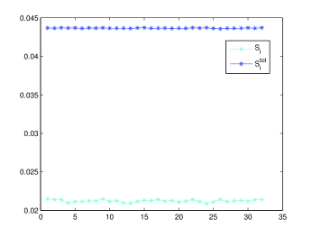
(a) Price

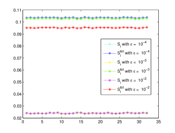
(b) Delta

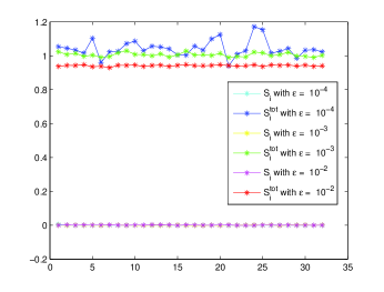
(c) Gamma

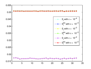
(d) Vega

Figure 1: European call option price $(a)$ and greeks $(b),(c),(d)$, SD, $D=32$. First order Sobol’ indices $S_{i}$ and total sensitivity indices $S_{i}^{tot}$ versus time step $i$.

(a) Price

(b) Delta

(c) Gamma

(d) Vega

Figure 2: Asian call option. Parameters as in Figure 1.

(a) Price

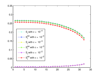
(b) Delta

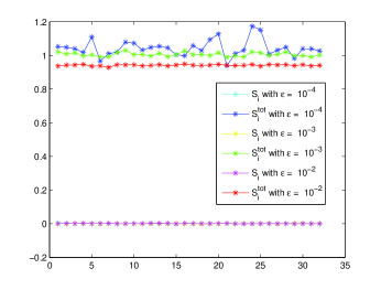
(c) Gamma

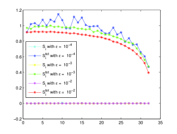
(d) Vega

Figure 3: Double Knock-out call option. Parameters as in Figure 1.

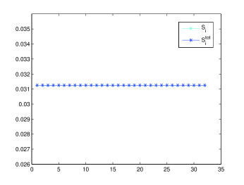
(a) Price

(b) Vega

Figure 4: Cliquet option. Parameters as in Figure 1. Delta and gamma are null for Cliquet options.

From these results we draw the following conclusions.

1. European option (Figure 1): price, delta and vega are type B functions, while gamma is type C function.

2. Asian option (Figure 2): price, and vega are type B functions, while delta and gamma are type C function.

3. Double KO option (Figure 3): price and all greeks are type C functions.

4. Cliquet option (Figure 4): price and vega are type B functions with $d_{S}=1$ (delta and gamma for a Cliquet option are null). We recall that $d_{S}=1$ means that there are no interactions among variables.

The analogous results of GSA for BBD are shown in Figures 5-8 and in Table 3.

Payoff	Function	$\mathbf{S_{i}/S_{i}^{tot}}$	$\mathbf{\sum_{i}S_{i}}$	$\mathbf{d_{T}}$	$\mathbf{d_{S}}$	$\mathbf{d_{A}}$	Effect of $\mathbf{\epsilon}$
European	Price	1	1	1	1	1	-
	Delta	1	1	1	1	1	no
	Gamma	1	1	1	1	1	no
	Vega	1	1	1	1	1	no
Asian	Price	0.853$\to$0.4	0.875	2	$\leq$2	1.13	-
	Delta	0.733$\to$0.01	0.778	4	$\leq$4	$1.68\to 1.43$	small
	Gamma	$10^{-2}\to 10^{-4}$	$0.022\to 10^{-4}$	32	32	$31\to 8$	high
	Vega	0.802$\to$0.03	0.827	2	$\leq$2	1.20	no
Double KO	Price	0.70$\to$0.01	0.70	$\simeq 2$	$\leq$2	1.63	-
	Delta	0.83$\to$0.01	0.83	2	$\leq$2	1.37	no
	Gamma	1	$1\to 0.95$	1	1	1.0	small
	Vega	$10^{-4}\to 0.2$	$10^{-6}\to 10^{-4}$	32	32	$4.8\to 3.9$	high
Cliquet	Price	0.978$\to$0.2	0.892	$\simeq 2$	$\leq 2$	1.19	-
	Vega	0.595$\to$0.001	0.32	$\simeq 32$	$\leq 32$	2.6	no

Table 3: Summary of GSA metrics and effective dimensions of prices and greeks for BBD scheme. Details as in Table 2.

(a) Price

(b) Delta

(c) Gamma

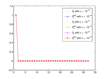
(d) Vega

Figure 5: European call option price $(a)$ and greeks $(b),(c),(d)$, BBD, $D=32$. First order Sobol’ indices $S_{i}$ and total sensitivity indices $S_{i}^{tot}$ versus time step $i$.

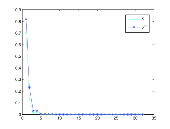
(a) Price

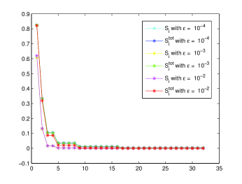
(b) Delta

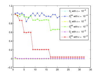
(c) Gamma

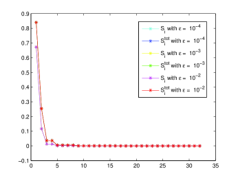
(d) Vega

Figure 6: Asian call option. Details as in Figure 5.

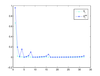
(a) Price

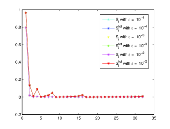
(b) Delta

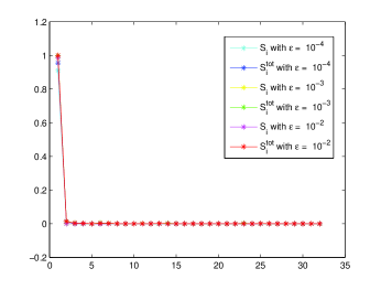
(c) Gamma

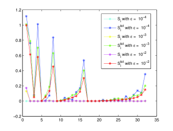
(d) Vega

Figure 7: Double Knock-out call option. Details as in Figure 5.

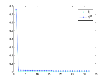
(a) Price

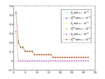
(b) Vega

Figure 8: Cliquet option. Details as in Figure 5.

From these results we draw the following conclusions.

1. European option (Figure 5): price and all greeks are type A functions with $d_{S}=1$. The value of sensitivity indexes for the first input, corresponding to the terminal value $t=T$, is $\simeq 1$, while the following variables have sensitivity indexes $\simeq 0$. Clearly, BBD is much more efficient than SD.

2. Asian option (Figure 6): price, delta and vega are type A functions. Comments as for the European option above. Gamma remains a type C function as for SD.

3. Double KO option (Figure 7): price, delta and gamma are type A functions. Comments as for the Asian option above. Vega remains a type C function as for SD.

4. Cliquet option (Figure 8): price is a type A function. Similarly to the European option, the value of sensitivity indexes for the first input, corresponding to the terminal value $t=T$, is $\simeq 1$, while the following values of $S_{i}$ are $\simeq 0$. Vega is a type C function, since the ratio $S_{i}/S_{i}^{tot}$ reaches small values revealing interacting variables. Thus in this case BBD is much less efficient than SD.

In conclusion, prices and greeks are always Type B or C functions for QMC+SD (Table 2), while they are predominantly Type A functions, with a few exceptions, for QMC+BBD (Table 3). In most cases switching from SD to BBD reduces the effective dimension in the truncation sense $d_{T}$.

The different efficiency of QMC+BBD vs QMC+SD is completely explained by the properties of Sobol’ low discrepancy sequences. The initial coordinates of Sobol’ LDS are much better distributed than the later high dimensional coordinates [Gla03, CMO97]. The BBD changes the order in which inputs (linked with time steps) are sampled. As follows from GSA, in most cases for BBD the low index variables (terminal values of time steps, mid-values and so on) are much more important than higher index variables. The BBD uses lower index, well distributed coordinates from each $D$-dimensional LDS vector to determine most of the structure of a path, and reserves other coordinates to fill in finer details. That is, well distributed coordinates are used for important variables and other not so well distributed coordinates are used for far less important variables. This results in a significantly improved accuracy of QMC integration. However, this technique does not always improve the efficiency of the QMC method as e.g. for Cliquet options: in this case GSA reveals that for SD all inputs are equally important and, moreover, there are no interactions among them, which is an ideal case for application of Sobol’ low discrepancy sequences; the BBD, on the other hand, favoring higher index variables destroys independence of inputs introducing interactions, which leads to higher values of $d_{S}$ and $d_{A}$. As a result, we observe degradation in performance of the QMC method.

4.3 Performance Analysis

In this section we compare the relative performances of MC and QMC techniques. This analysis is crucial to establish if QMC outperforms MC, and in what sense.

Firstly, following the suggestion of [Jac01], Section 14.4, we analyze convergence diagrams for prices and greeks, showing the dependence of the MC simulation error upon the number of MC paths. The results for the four payoffs are shown in Figures 9-12 .

(a) Price

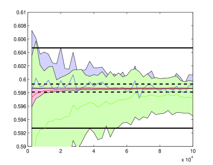
(b) Delta

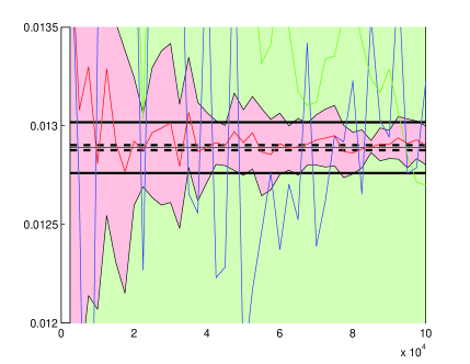
(c) Gamma

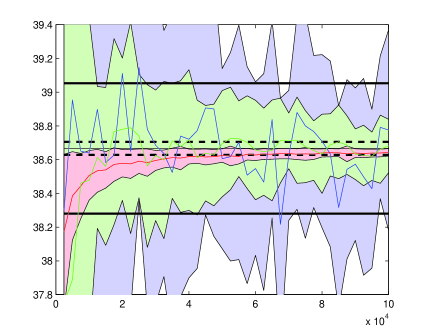
(d) Vega

Figure 9: European call option price $(a)$ and greeks $(b),(c),(d)$ convergence diagrams versus number of simulated paths for MC+SD with antithetic variables (solid blue line), QMC+SD (solid green line) and QMC+BBD (solid red line). Shaded areas represent 3-sigma errors around the corresponding run (solid line). 1% and 0.1% accuracy regions are marked by horizontal black solid and dashed lines, respectively. Number of dimensions is $D=32$. Shift parameter is $\epsilon=10^{-3}$.

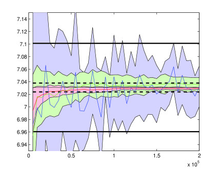
(a) Price

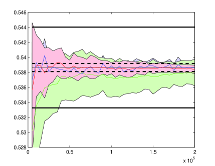
(b) Delta

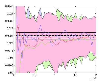
(c) Gamma

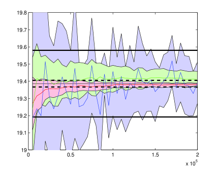
(d) Vega

Figure 10: Asian call option. $\epsilon=5\times 10^{-3}$. Other details as in Figure 9.

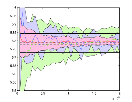
(a) Price

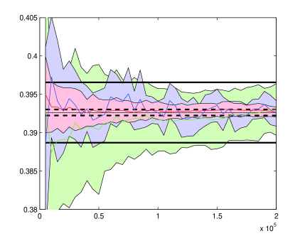
(b) Delta

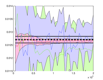
(c) Gamma

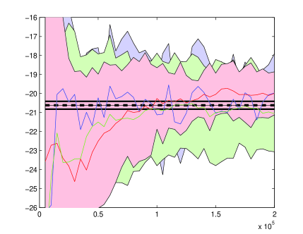
(d) Vega

Figure 11: Double Knock-out call option. Details as in Figure 10.

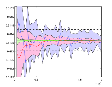
(a) Price

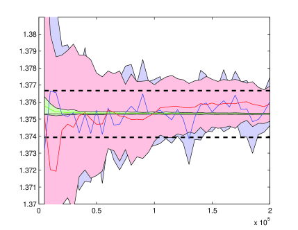
(b) Vega

Figure 12: Cliquet option. Details as in Figure 10.

We observe what follows.

1. European option (Figure 9): QMC+BBD outperforms both QMC+SD and MC+SD in all cases (the 3-sigma regions for QMC+BBD are systematically smaller). We also note that for price, delta and vega, the QMC+BBD convergence is practically monotonic, which makes on-line error approximation possible. For gamma, the QMC+BBD convergence is much less oscillating than for MC+SD.

2. Asian option (Figure 10): QMC+BBD outperforms both QMC+SD and MC+SD for price and vega. For delta, QMC with both SD and BBD is marginally better than MC+SD. For gamma, QMC with both SD and BBD has nearly the same efficiency as MC+SD. The QMC+BBD convergence is also smoother for price, delta and vega.

3. Double KO option (Figure 11): QMC+BBD outperforms both QMC+SD and MC+SD in all cases.

4. Cliquet option (Figure 12): QMC+SD outperforms QMC+BBD and MC+SD in all cases. QMC+BBD outperforms MC+SD only for price.

Next, we analyze the relative performance of QMC vs MC in terms of convergence rate. We plot in Figures 13-16 the root mean square error, eq. (2.24), versus the number of MC scenarios $N$ in Log-Log scale. In all our tests we have chosen an appropriate range for $N$ such that, in the computation of greeks, the bias term is negligible with respect to the variance term (see Appendix A for details). Hence, the observed relations are, with good accuracy, linear, therefore the power law (2.23) is confirmed, and the convergence rates $\alpha$ can be extracted as the slopes of the regression lines. Furthermore, also the intercepts of regression lines provide useful information about the efficiency of the QMC and MC methods: in fact, lower intercepts mean that the simulated value starts closer to the exact value. The resulting slopes and intercepts from linear regression are presented in tabs. 4 and 5 for all test cases.

Payoff	Function	MC+SD	QMC+SD	QMC+BBD
European	Price	-0.3 $\pm$ 0.1	-0.2 $\pm$ 0.1	-0.84 $\pm$ 0.01
	Delta	-2.0 $\pm$ 0.1	-1.6 $\pm$ 0.1	-2.64 $\pm$ 0.01
	Gamma	-2.0 $\pm$ 0.1	-2.1 $\pm$ 0.1	-2.8 $\pm$ 0.2
	Vega	0.4 $\pm$ 0.1	0.4 $\pm$ 0.1	-0.13 $\pm$ 0.01
Asian	Price	-0.5 $\pm$ 0.1	-0.5 $\pm$ 0.1	-1.0 $\pm$ 0.1
	Delta	-2.2 $\pm$ 0.1	-1.7 $\pm$ 0.1	-1.9 $\pm$ 0.1
	Gamma	-2.1 $\pm$ 0.2	-2.1 $\pm$ 0.1	-2.0 $\pm$ 0.1
	Vega	0.1 $\pm$ 0.1	-0.1 $\pm$ 0.1	-0.4 $\pm$ 0.1
Double KO	Price	-0.4 $\pm$ 0.1	-0.3 $\pm$ 0.1	-0.7 $\pm$ 0.1
	Delta	-1.8 $\pm$ 0.1	-1.6 $\pm$ 0.1	-2.1 $\pm$ 0.1
	Gamma	-2.4 $\pm$ 0.1	2.1 $\pm$ 0.1	-2.9 $\pm$ 0.1
	Vega	1.1 $\pm$ 0.1	1.3 $\pm$ 0.1	1.3 $\pm$ 0.2
Cliquet	Price	-2.4 $\pm$ 0.1	-3.2 $\pm$ 0.1	-2.5 $\pm$ 0.3
	Vega	-2.0 $\pm$ 0.1	-2.7 $\pm$ 0.1	-1.7 $\pm$ 0.2

Table 4: Intercepts from linear regression with their errors, for MC+SD with antithetic variables, QMC+SD and QMC+BBD, $L=30$ runs. Results are shown for $N=10^{2.5}$ paths.

Payoff	Function	MC+SD	QMC+SD	QMC+BBD
European	Price	-0.46 $\pm$ 0.03	-0.71 $\pm$ 0.03	-0.901 $\pm$ 0.003
	Delta	-0.49 $\pm$ 0.03	-0.56 $\pm$ 0.02	-0.926 $\pm$ 0.004
	Gamma	-0.51 $\pm$ 0.02	-0.51 $\pm$ 0.01	-0.98 $\pm$ 0.04
	Vega	-0.45 $\pm$ 0.03	-0.69 $\pm$ 0.03	-0.869 $\pm$ 0.003
Asian	Price	-0.50 $\pm$ 0.02	-0.70 $\pm$ 0.03	-0.85 $\pm$ 0.01
	Delta	-0.49 $\pm$ 0.03	-0.59 $\pm$ 0.02	-0.61 $\pm$ 0.03
	Gamma	-0.53 $\pm$ 0.05	-0.49 $\pm$ 0.03	-0.50 $\pm$ 0.03
	Vega	-0.51 $\pm$ 0.02	-0.64 $\pm$ 0.04	-0.75 $\pm$ 0.01
Double KO	Price	-0.49 $\pm$ 0.03	-0.49 $\pm$ 0.02	-0.56 $\pm$ 0.03
	Delta	-0.49 $\pm$ 0.02	-0.52 $\pm$ 0.03	-0.55 $\pm$ 0.02
	Gamma	-0.45 $\pm$ 0.03	-0.51 $\pm$ 0.02	-0.61 $\pm$ 0.02
	Vega	-0.50 $\pm$ 0.03	-0.53 $\pm$ 0.02	-0.57 $\pm$ 0.04
Cliquet	Price	-0.51 $\pm$ 0.02	-1.00 $\pm$ 0.03	-0.72 $\pm$ 0.09
	Vega	-0.48 $\pm$ 0.02	-0.86 $\pm$ 0.04	-0.62 $\pm$ 0.04

Table 5: Slopes from linear regression with their errors, as in Table 4. In a few cases we show three decimals since the MC error is lower.

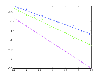
(a) Price

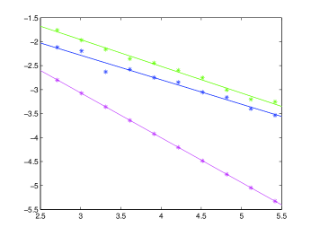
(b) Delta

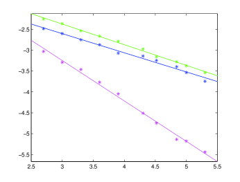
(c) Gamma

(d) Vega

Figure 13: European call option price $(a)$ and greeks $(b),(c),(d)$, Log-Log plots of error $\varepsilon_{N}$ versus number of simulated paths $N=2^{p},\;p=9,\ldots,18$, $D=32$, $\epsilon=10^{-3}$, $L=30$ runs: MC+SD with antithetic variables (blue), QMC+SD (green), QMC+BBD (magenta). Linear regression lines are also shown.

(a) Price

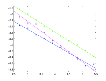
(b) Delta

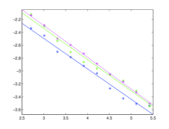
(c) Gamma

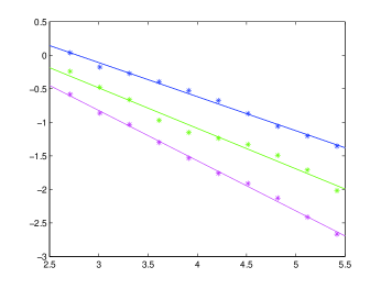
(d) Vega

Figure 14: Asian call option. $\epsilon=5\times 10^{-3}$. Other details as in Figure 13.

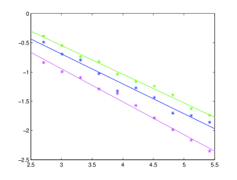
(a) Price

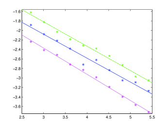
(b) Delta

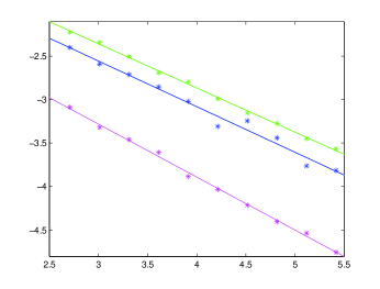
(c) Gamma

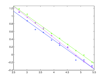
(d) Vega

Figure 15: Double Knock-out call option. Details as in Figure 14.

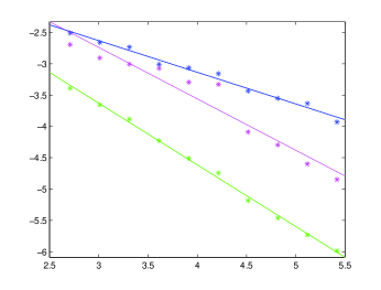
(a) Price

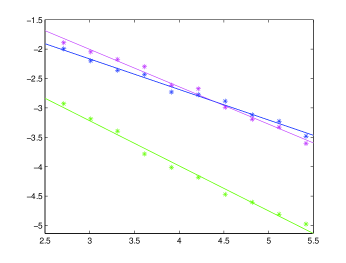
(b) Vega

Figure 16: Cliquet option. Details as in Figure 14.

We observe what follows.

1. European option (Figure 13): QMC+BBD outperforms other methods, having the highest rate of convergence $\alpha$ and the smallest intercept. QMC+SD for price and vega has higher rate of convergence $\alpha$ but also somewhat higher intercepts than MC+SD. It performs marginally better for delta and as good as MC+SD for gamma in terms of $\alpha$ values.

2. Asian option (Figure 14): for price and vega QMC+BBD and QMC+SD have higher $\alpha$ than MC+ SD, with QMC+BBD being the most efficient. They also have slightly higher $\alpha$ for delta, but both have lower intercepts than MC. For gamma all methods show similar convergence.

3. Double KO option (Figure 15): QMC+BBD has the highest $\alpha$ although its highest value $\alpha=0.61$ (for gamma) is lower than $\alpha$ for European and Asian options (with an exception of gamma of Asian option). Its intercepts for price, delta and gamma also have the lowest values among all methods. The QMC+SD is as efficient as MC.

4. Cliquet option (Figure 16): QMC+SD has the highest $\alpha$, close to 1.0. It also has the lowest intercepts among all methods. QMC+BBD has higher $\alpha$ but similar intercepts in comparison with MC+SD.

We stress that slopes and intercepts shown in the previous figures 13-16 do not depend on the details of the simulations, in particular the MC seed or the LDS starting point, since we are averaging over $L=30$ runs.

In conclusion, QMC+BBD generally outperforms the other methods, except for asian gamma where all methods show similar convergence properties and Cliquet option for which QMC+SD is the most efficient method.

4.4 Speed-Up Analysis

A typical question with Monte Carlo simulation is “how many scenarios are necessary to achieve a given precision?”. When comparing two numerical simulation methods, the typical question becomes “how many scenarios may I save using method B instead of method A, preserving the same precision?”.

A useful measure of the relative computational performance of two numerical methods is the so called speed-up $S_{*}(a)$ [KMRZ98a, PT96]. It is defined as

$$S_{*}^{(i,j)}(a)=\frac{N_{*}^{(j)}(a)}{N_{*}^{(i)}(a)}\,,$$ (4.6)

where, in our context, $N_{*}^{(i)}(a)$ is the number of scenarios using the i-th computational method (MC+SD, QMC+SD, or QMC+BBD) needed to reach and maintain a given accuracy $a$ w.r.t. exact or almost exact results. Thus, the speed-up $S_{*}(a)$ quantifies the computational gain of method $i$ w.r.t. method $j$.

The speed-up $N_{*}$ could be evaluated through direct simulation, but this would be extremely computationally expensive. Thus we resort to the much simpler algorithm described in Appendix B.

Payoff	Function	QMC+SD		QMC+BBD		QMC+BBD
		vs MC+SD		vs MC+SD		vs QMC+SD
		$a=1\%$	$a=0.1\%$	$a=1\%$	$a=0.1\%$	$a=1\%$	$a=0.1\%$
European	Price	3	6	30	140	10	20
	Delta	0.3	0.5	20	100	60	200
	Gamma	0.5	0.5	200	1000	600	5000
	Vega	5	6	50	140	10	20
Asian	Price	5	10	30	100	5	10
	Delta	0.2	0.5	0.4	2	2	5
	Gamma	0.5	-	0.5	-	1	-
	Vega	6	10	30	100	5	10
Double KO	Price	0.5	0.8	5	10	10	15
	Delta	0.5	1	5	20	10	20
	Gamma	0.7	1.3	110	650	150	500
	Vega	0.5	0.5	1.5	1.5	3	3
Cliquet	Price	10	100	1	10	0.1	0.1
	Vega	20	100	0.5	1	0.02	0.01

Table 6: Speed-up $S_{*}(a)$ of the various numerical methods w.r.t. each other (see columns), for different option types. The shift $\epsilon$ for finite differences is the same as used in the previous sections. Missing values of $S_{*}$ mean that the required accuracy cannot be reached since it is smaller than the bias.

We show in Table 6 the results of the speed-up analysis obtained for all methods and for all option types described in the previous sections. The speed-up measure clearly shows the relative efficiencies of the methods considered for each case. In general, QMC+BBD largely outperforms the other methods, with a speed-up factor up to $10^{3}$ (European and Barrier gamma) and a few exceptions (Asian delta and gamma, Cliquet). QMC+SD is the best method for Cliquet. We notice in particular that, in most cases, a ten-fold increase of the accuracy $a$ results in a two-fold increase of speed-up $S_{*}(a)$. However, in a few cases (gamma for European and Cliquet options), such an increase can result in up to ten-folds increase of $S_{*}(a)$.

The difficulty with speed-up is the possible non-monotonicity of the convergence plot for a given numerical methods. Unfortunately, our algorithm to estimate speed-up in Appendix B cannot capture unexpected fluctuations of the convergence plot, which could lead to underestimate $N_{*}(a)$. However, we believe that the choice of the 3-sigma confidence interval in eq. (B.1) makes our speed-up analysis reliable, at least when coupled with the stability analysis described in the next Section 4.5.

4.5 Stability Analysis

We have already observed that QMC convergence is often smoother than MC (see Figures 9-12): such monotonicity and stability guarantee better convergence for a given number of paths $N$. In order to quantify monotonicity and stability of the various numerical techniques, the following strategy is used: we divide the range of path simulations $N$ in 10 windows of equal length, and we compute the sample mean $m_{i}$ and the sample standard deviation (“volatility”) $s_{i}$ for each window $i$. Then, log-returns $\log(m_{i}/m_{i-1})$ and volatilities $s_{i}$, for $i=2,\ldots,10$, are used as measures of, respectively, monotonicity and stability: “monotonic” convergence will show non oscillating log-returns converging to zero, “stable” convergence will show low and almost flat volatility. We performed stability analysis for MC and QMC methods. For QMC we used two different generators: pure QMC with Broda generator and randomized Quasi Monte Carlo (rQMC) with Matlab generator. The results are shown in Figures 17-20.

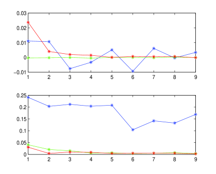
(a) Price

(b) Delta

(c) Gamma

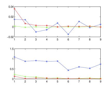
(d) Vega

Figure 17: Log-returns (upper plots) and volatilities (lower plots) of European call option price $(a)$ and greeks $(b),(c),(d)$, for $D=32$, $\epsilon=10^{-3}$, MC+SD (blue), rQMC+BBD (green) and pure QMC+BBD (red). The number of simulation paths ranges from 100 to 10,000 grouped in 10 windows each containing 10 samples (x-axis).

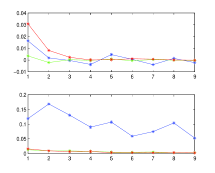
(a) Price

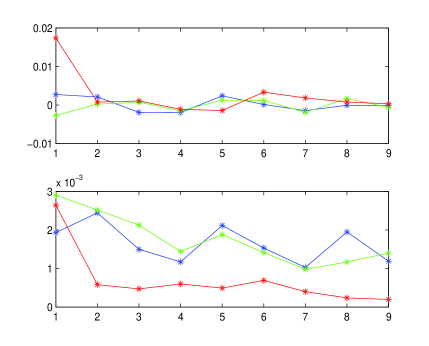
(b) Delta

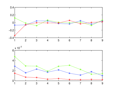
(c) Gamma

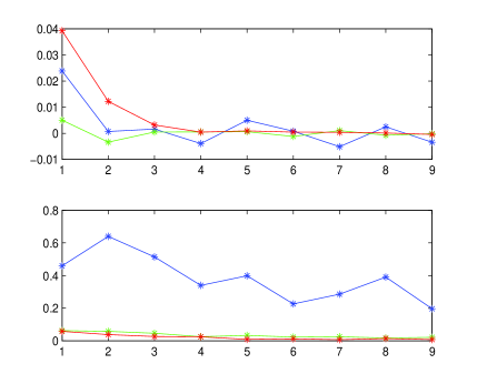
(d) Vega

Figure 18: Asian call option. $\epsilon=5\times 10^{-3}$. Other details as in Figure 17.

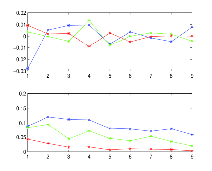
(a) Price

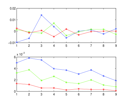
(b) Delta

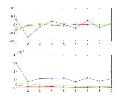
(c) Gamma

(d) Vega

Figure 19: Double Knock-out call option. Details as in Figure 18.

(a) Price

(b) Vega

Figure 20: Cliquet option. QMC and rQMC with SD were used here. Other details as in Figure 18.

(a) Price

(b) Delta

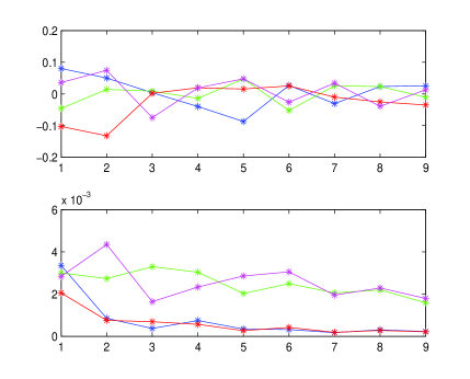
(c) Gamma

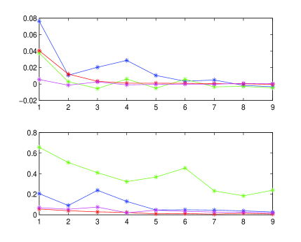
(d) Vega

Figure 21: Asian call option with $D=252$, $\epsilon=5\times 10^{-3}$. Results are shown for rQMC+SD+Matlab (green) and rQMC+BBD+Matlab (magenta), and QMC+SD+Broda (blue) and QMC+BBD+Broda (red).

We observe that, in general, QMC+Broda and rQMC+Matlab are more monotonic and stable than MC+SD. However, this fact is less evident for Asian delta and gamma, where QMC lacks monotonicity and stability w.r.t. MC, with QMC+BRODA being slightly more stable than rQMC+Matlab. As we know from the results of GSA for this case, higher order interactions are present and the effective dimensions are large (see Table 3).

In order to understand also the effect of dimension $D$ on monotonicity and stability, we run a similar experiment for an Asian option with $D=252$ fixing dates using both QMC and rQMC with SD and BBD. The results are shown in Figure 21. We observe that pure QMC with Broda generator preserves monotonicity and stability much more than randomized QMC based on Matlab generator for all cases including delta and gamma, with QMC+BBD+Broda showing the best stability. It is also interesting to note that the increase in dimension resulted in the decrease in the effective dimensions for the case of the BBD (but not for the SD).

We conclude that good high-dimensional LDS generators are crucial to obtain a smooth monotonic and stable convergence of the Monte Carlo Simulation in high effective dimensional problems.

5 Conclusions

In this work we presented an updated overview of the application of Quasi Monte Carlo (QMC) and Global Sensitivity Analysis (GSA) methods in Finance, w.r.t. standard Monte Carlo (MC) methods. In particular, we considered prices and greeks (delta, gamma, vega) for selected payoffs with increasing degree of complexity and path-dependency (European Call, Geometric Asian Call, Double Barrier Knock-Out, Cliquet options). We compared standard discretization (SD) vs Brownian bridge discretization (BBD) schemes of the underlying stochastic diffusion process, and different sampling of the underlying distribution using pseudo random vs high dimensional Sobol’ low discrepancy sequences. We applied GSA and we performed detailed and systematic analysis of convergence diagrams, error estimation, performance, speed-up and stability of the different MC and QMC simulations.

The GSA results in Section 4.2 revealed that effective dimensions associated to QMC+BBD simulations are generally lower than those associated to MC+SD simulations, and how much such dimension reduction acts for different payoffs and greeks (Figures 1-8 and Tables 2-3). Effective dimensions, being linked with the structure of ANOVA decompositions (the number of important inputs, importance of high order interactions) fully explained the superior efficiency of QMC+BBD due to the specifics of Sobol’ sequences and BBD. The BBD is generally more efficient than SD, but with some exceptions, Cliquet options in particular.

The performance analysis results in Section 4.3 showed that QMC+BBD outperforms MC+SD in most cases, showing faster and more stable convergence to exact or almost exact results (Figures 9-12, 13-16, and Tables 4-5), with some exceptions such as Asian option gamma where all methods showed similar convergence properties.

The speed-up analysis results in Section 4.4 confirmed that the superior performance of QMC+BBD allows significative reduction of the number of scenarios to achieve a given accuracy, leading to significative reduction of computational effort (Table 6). The size of the reduction scales up to $10^{3}$ (European and Double KO gamma), with a few exceptions (Asian delta and gamma, Cliquet).

Finally, the stability analysis results in 4.5 confirmed that QMC+BBD simulations are generally more stable and monotonic than MC+SD, with the exception of Asian delta and gamma (Figures 17-21).

We conclude that the methodology presented in this paper, based on Quasi Monte Carlo, high dimensional Sobol’ low discrepancy generators, efficient discretization schemes, global sensitivity analysis, detailed convergence diagrams, error estimation, performance, speed-up and stability analysis, is a very promising technique for more complex problems in finance, in particular, credit/debt/funding/capital valuation adjustments (CVA/DVA/FVA/KVA) and market and counterparty risk measures, based on multi-dimensional, multi-step Monte Carlo simulations of large portfolios of trades. Such simulations can run, in typical real cases, $\sim 10^{2}$ time simulation steps, $\sim 10^{3}$ (possibly correlated) risk factors, $\sim 10^{3}-10^{4}$ MC scenarios, $\sim 10^{4}-10^{5}$ trades, $60$ years maturity, leading to a nominal dimensionality of the order $D\sim 10^{5}$, and to a total of $10^{9}-10^{11}$ evaluations. Unfortunately, a fraction $\sim 1\%$ of exotic trades may require distinct MC simulations for their evaluation, nesting another set of $\sim 10^{3}-10^{5}$ MC scenarios, thus leading up to $10^{14}$ evaluations. Finally, hedging CVA/DVA/FVA/KVA valuation adjustments w.r.t. to their underlying risk factors (typically credit/funding curves) also requires the computation of their corresponding greeks w.r.t. each term structure node, adding another $\sim 10^{2}$ simulations. This is the reason why the industry is continuously looking for advanced techniques to reduce computational times: grid computing, GPU computing, adjoint algorithmic differentiation (AAD), etc. (see e.g. [She15]).

We argue that, using QMC sampling (instead of MC) to generate the scenarios of the underlying risk factors and to price exotic trades may significantly improve the accuracy, the performance and the stability of such monster-simulations, as shown by preliminary results on real portfolios [BKS14]. Furthermore, GSA should suggest how to order the risk factors according to their relative importance, thus reducing the effective dimensionality. Such applications will need further research.

Appendix A Error Optimization in Finite Difference Approximation

There are two contributions to the root mean square error when greeks are computed by MC/QMC simulation via finite differences: variance and bias [Gla03]. The first source of uncertainty comes from the fact that we are computing prices through simulation over a finite number of scenarios, while the latter is due to the approximation of a derivative with a finite difference. In order to minimize the variance, we use the same set of (quasi)random numbers for the computation of $V(\theta)$, $V(\theta+h)$ and $V(\theta-h)$, where $V$ is the option price, the parameter $\theta$ is the spot for delta and gamma or the volatility for vega and $h$ is the increment on $\theta$. In order to minimize the bias of the finite differences we use central differences, so that it is of the order $h^{2}$. The increments $h$ are chosen to be $h=\epsilon S_{0}$, for $\Delta$ and $\Gamma$, and $h=\epsilon$, for $\mathcal{V}$, for a given “shift parameter” $\epsilon$. The choice of the appropriate $\epsilon$ is guided by the following considerations. The MC/QMC root mean square error estimate of finite differences is given by [Gla03]:

$$\varepsilon=\sqrt{\frac{c}{N^{2\alpha}h^{\beta}}+b^{2}h^{4}}\,.$$ (A.1)

The first term in the square root is a “statistical” error related to the variance $c$. It depends on $N$ as well as on $\epsilon$. $\alpha=0.5$ for MC and, usually, $0.5<\alpha<1$ for QMC, while $\beta=1$ for first derivatives and $\beta=3$ for second derivatives. The second term is the systematic error due to the bias of finite differences: it is independent of $N$ but it depends on $\epsilon$. The constant $b$ is given by $b=\frac{1}{6}\frac{\partial^{3}V}{\partial\theta^{3}}(\theta)$ for central differences of the first order (delta and vega) and $b=\frac{1}{12}\frac{\partial^{4}V}{\partial\theta^{4}}(\theta)$ for central differences of the second order (gamma). One can see that, when $h$ is decreasing, the bias term decreases as well while the variance term increases, therefore we fine tune $h$ in such a way that the variance term is not too high in the relevant range for $N$, while the bias term remains negligible so that (A.1) follows approximately a power law. We note that the optimal value of $h$ is not observed to vary too much with $N$ in the range used for our tests. Indeed, it can be computed analytically from (A.1) as the minimum of $\varepsilon$:

$$h_{N}=\left(\frac{\beta c}{4b^{2}N^{2\alpha}}\right)^{\frac{1}{\beta+4}}\,.$$ (A.2)

We see that the powers $\frac{1}{5}$ and $\frac{1}{7}$ (corresponding to $\beta=1$ and $\beta=3$ respectively) largely flatten $h_{N}$ as a function of $N$.

Appendix B Speed-Up Computation

We identify the number of scenarios $N_{*}^{(i)}(a)$ in eq. (4.6) using the i-th computational method needed to reach and maintain a given accuracy $a$ as the first number of simulated paths such that, for any $N>N_{*}$

$$V-a\leq V_{N}\pm 3\,\varepsilon\leq V+a\,,$$ (B.1)

where $V$ and $V_{N}$ are respectively the exact and simulated values of prices or greeks and $\varepsilon$ is the standard error. The threshold $N_{*}$ could be evaluated through direct simulation, but this would be extremely computationally expensive. Extracting $N_{*}$ from plots defined by (2.23) can’t be applied directly because, in the case of greeks, such plots are correct only for a limited range of values of $N$, i.e. as long as the bias term in (A.1) does not become dominant. Extrapolating $N_{*}$ from plots to high values of $N$ is necessary to compute speed-up, but the relation between RMSE and $N$ would not be linear anymore. We therefore follow a different procedure to determine $N_{*}$. Equation (A.1) can be rewritten as

$$\log\varepsilon=k-\alpha\log N,$$ (B.2)

where $k=\frac{1}{2}\log\frac{c}{h^{\beta}}$ and $\alpha$ are, respectively, the intercept and the slope computed from linear regressions on $\varepsilon_{N}$ given by (2.24). Therefore, $N_{*}$ is found by imposing

$$a=3\,\sqrt{\frac{e^{2k}}{N_{*}^{2\alpha}}+b^{2}h^{4}},$$ (B.3)

and is given by

$$N_{*}(h,a)=\left(\frac{9\,e^{2k_{h}}}{a^{2}-9b^{2}h^{4}}\right)^{\frac{1}{2\alpha_{h}}}.$$ (B.4)

We have written $k_{h}$ and $\alpha_{h}$ in order to stress that they also depend on the choice of $h$ made while carrying out the tests in Section 4: this dependence on $h$ can be stronger than the explicit dependence in (B.4). Constant $b$ is computed from derivatives of $V$ (see discussion after presenting equation (A.1) ); $k$ and $\alpha$ are the intercepts and slopes correspondingly taken from plots (Figures 13-16): this is possible, since these plots are obtained for a range of $N$ such that the second term in (A.1) is negligible. It is clear that the domain of $N_{*}$ is limited to $a>3bh^{2}$. In the case of prices, equation (B.4) simplifies to

$$N_{*}(a)=\left(\frac{3e^{k_{h}}}{a}\right)^{\frac{1}{\alpha_{h}}}\,.$$ (B.5)

References

- [BBG97] Phelim P. Boyle, Mark Broadie, and Paul Glasserman. Simulation Methods for Security Pricing. Journal of Economic Dynamics and Control, 21:1267–1321, 1997.
- [BKS14] Marco Bianchetti, Sergei Kucherenko, and Stefano Scoleri. Better Pricing and Risk Management with High Dimensional Quasi Monte Carlo. WBS 10th Fixed Income Conference, September 2014.
- [BM06] Damiano Brigo and Fabio Mercurio. Interest-Rate Models - Theory and Practice. Springer, 2nd edition, 2006.
- [Boy77] Phelim P. Boyle. Options: a Monte Carlo Approach. Journal of Financial Economics, 4:323–338, 1977.
- [BRO] BRODA Ltd., High-dimensional Sobol’ sequence generators.
- [CMO97] R. E. Caflish, W. Morokoff, and A. Owen. Valuation of mortgage-backed securities using Brownian bridges to reduce effective dimension. The Journal of Computational Finance, 1(1):27–46, 1997.
- [Duf01] Darrel Duffie. Dynamic Asset Pricing Theory. Princeton University Press, 3rd edition, 2001.
- [Gla03] Paul Glasserman. Monte Carlo Methods in Financial Engineering. Springer, 2003.
- [Jac01] Peter Jackel. Monte Carlo Methods in Finance. Wiley, 2001.
- [KFSM11] Sergei Kucherenko, Balazs Feil, Nilay Shah, and Wolfgang Mauntz. The identification of model effective dimensions using global sensitivity analysis. Reliability Engineering and System Safety, 96:440–449, 2011.
- [KMRZ98a] Alexander Kreinin, Leonid Merkoulovitch, Dan Rosen, and Michael Zerbs. Measuring Portfolio Risk Using Quasi Monte Carlo Methods. Algo Research Quarterly, 1(1), September 1998.
- [KMRZ98b] Alexander Kreinin, Leonid Merkoulovitch, Dan Rosen, and Michael Zerbs. Principal Component Analysis in Quasi Monte Carlo Simulation. Algo Research Quarterly, 1(2), December 1998.
- [KP95] P.E. Kloden and E. Platen. Numerical Solutions of Stochastic Differential Equations. Springer, Berlin, Heidelberg, New York, 1995.
- [KS07] Sergei Kucherenko and Nilay Shah. The Importance of being Global. Application of Global Sensitivity Analysis in Monte Carlo option Pricing. Wilmott Magazine, 4, 2007.
- [KTA12] S. Kucherenko, S. Tarantola, and P. Annoni. Estimation of global sensitivity indices for models with dependent variables. Computer Physics Communications, 183:937–946, 2012.
- [Lab66] Los Alamos Scientific Laboratory. Fermi invention rediscovered at LASL. The Atom, pages 7–11, October 1966.
- [LO00] C. Lemieux and A. Owen. Quasi-regression and the relative importance of the anova component of a function. In: Fang K-T, Hickernell FJ, Niederreiter H, editors. Monte Carlo and quasi-Monte Carlo., 2000.
- [LO06] R. Liu and A.B. Owen. Estimating mean dimensionality of analysis of variance decompositions. Journal of the American Statistical Association, 101(474):712–721, 2006.
- [Met87] Nicholas Metropolis. The beginning of the Monte Carlo Method. Los Alamos Science, pages 125–130, 1987. Special Issue dedicated to Stanislaw Ulam.
- [MF99] Maurizio Mondello and Maurizio Ferconi. Quasi Monte Carlo Methods in Financial Risk Management. Tech Hackers, Inc., 1999.
- [MN98] M. Matsumoto and T. Nishimura. Mersenne twister: a 623-dimensionally equidistributed uniform pseudo-random number generator. ACM Transactions on Modeling and Computer Simulation, 8(1):3–30, 1998.
- [Nie88] H. Niederreiter. Low-discrepancy and low-dispersion sequences. Journal of Number Theory, 30:51?70, 1988.
- [Oks92] B. Oksendal. Stochastic Differential Equations: An Introduction with Applications. Springer, Berlin, 1992.
- [Owe93] A.B. Owen. Variance and discrepancy with alternative scramblings. ACM Transactions on Modeling and Computer Simulation, 13:363–378, 1993.
- [Owe03] A. Owen. The dimension distribution and quadrature test functions. Stat Sinica, 13:1–17, 2003.
- [Pap01] A. Papageorgiou. The Brownian Brisge does not offer a Consistent Advantage in Quasi-Monte Carlo Integration. Journal of complexity, 2001.
- [PP99] A. Papageorgiou and S. Paskov. Deterministic Simulation for Risk Management. Journal of Portfolio Management, pages 122–127, May 1999.
- [PT95] S. H. Paskov and J. F. Traub. Faster Valuation of Financial Derivatives. The Journal of Portfolio Management, pages 113–120, Fall 1995.
- [PT96] A. Papageorgiou and J. F. Traub. New Results on Deterministic Pricing of Financial Derivatives. presented at “Mathematical Problems in Finance”, Institute for Advanced Study, Princeton, New Jersey, April 1996.
- [SAA+10] A. Saltelli, P. Annoni, I. Azzini, F. Campolongo, M. Ratto, and S. Tarantola. Variance based sensitivity analysis of model output. Design and estimator for the total sensitivity index. Computer Physics Communication, 181:259–270, 2010.
- [SAKK12] Ilya M. Sobol’, Danil Asotsky, Alexander Kreinin, and Sergei Kucherenko. Construction and Comparison of High-Dimensional Sobol’ Generators. Wilmott Magazine, Nov:64–79, 2012.
- [Sal02] A. Saltelli. Making best use of model evaluations to compute sensitivity indices. Comput. Phys. Commun., 145:280–297, 2002.
- [She15] Nazneen Sherif. AAD vs GPUs: banks turn to maths trick as chips lose appeal. Risk, January 2015.
- [SK05a] Ilya M. Sobol’ and Sergei Kucherenko. Global Sensitivity Indices for Nonlinear Mathematical Models. Review. Wilmott Magazine, 1:56–61, 2005.
- [SK05b] Ilya M. Sobol’ and Sergei Kucherenko. On the Global Sensitivity Analysis of Quasi Monte Carlo Algorithms. Monte Carlo Methods and Applications, 11(1):1–9, 2005.
- [Sob67] Ilya M. Sobol’. On the distribution of points in a cube and the approximate evaluation of integrals. Comp Math Math Phys, 7:86–112, 1967.
- [Sob01] Ilya M. Sobol’. Global Sensitivity Indices for Nonlinear Mathematical Models and their Monte Carlo Estimates. Mathematics and Computers in Simulation, 55:271–280, 2001.
- [SS14] Ilya M. Sobol’ and Boris V. Shukhman. Quasi-Monte Carlo: A high-dimensional experiment. Monte Carlo Methods and Applications, May:167–171, 2014.
- [VN51] John Von Neumann. Monte Carlo Method, volume 12 of Applied Mathematics Series, chapter 13: Various Techniques Used in Connection With Random Digits, pages 36–38. U.S. Department of Commerce, National Bureau of Standards, June 1951.
- [Wan09] Xiaoqun Wang. Dimension Reduction Techniques in Quasi-Monte Carlo Methods for Option Pricing. INFORMS Journal on Computing, 21(3):488–504, Summer 2009.
- [Wil06] Paul Wilmott. Paul Wilmott on Quantitative Finance. John Wiley & Sons, Ltd, 2 edition, 2006.