KCL-PH-TH/2015-17, LCTS/2015-08, CERN-PH-TH/2015-072

We develop a universal approach to the one-loop effective field theory (EFT) using the Covariant Derivative Expansion (CDE) method. We generalise previous results to include broader classes of UV models, showing how expressions previously obtained assuming degenerate heavy-particle masses can be extended to non-degenerate cases. We apply our method to the general MSSM with non-degenerate stop squarks, illustrating our approach with calculations of the coefficients of dimension-6 operators contributing to the $hgg$ and $h\gamma\gamma$ couplings, and comparing with exact calculations of one-loop Feynman diagrams. We then use present and projected future sensitivities to these operator coefficients to obtain present and possible future indirect constraints on stop masses. The current sensitivity is already comparable to that of direct LHC searches, and future FCC-ee measurements could be sensitive to stop masses above a TeV. The universality of our one-loop EFT approach facilitates extending these constraints to a broader class of UV models.

April 2015

1 Introduction

In view of the overall consistency between the current measurements of particle properties and predictions in the Standard Model (SM), a common approach to the analysis of present and prospective future data is to describe them via an effective field theory (EFT) in which the renormalizable SM $d=4$ Lagrangian is supplemented with higher-dimensional terms composed from SM fields [1, 2]. To the extent that this new physics has a mass scale that is substantially higher than the energy scale of the available measurements [3], the EFT approach is a powerful way to constrain possible new physics beyond the SM (BSM) that is model-independent [4, 5, 6]. The $d=6$ operators in this Effective SM (ESM) were first classified in [1], with a complete basis using equations of motion to eliminate redundancies [2] being first presented in [9]. There have been many studies of various aspects of these dimension-6 operators , and a short review can be found in [16].

The EFT approach may well be a good approximation if the new physics affects precision observables at the tree level, or if it is strongly-interacting. In these cases the new physics mass scale is likely to be relatively high, and considering the lowest-dimensional EFT operators may well be sufficient. However, the EFT approach may have limitations if the new physics has effects only at the loop level, or is weakly interacting. In these cases, the EFT approach may be sensitive only to new physics at some relatively low mass scale, and the new physics effects may not be characterised well by considering simply the lowest-dimensional EFT operators.

Examples in the first, ‘safer’ category may include certain models with extended Higgs sectors [15], such as two-Higgs-doublet models, or some composite models. Examples in the second category may include the loop effects of supersymmetric models. However, even in this case it is possible that precision electroweak and Higgs data may provide interesting constraints on the possible masses of stop squarks, which have relatively large Yukawa couplings to the SM Higgs field. In particular, the EFT approach may be useful in the framework of ‘natural’ supersymmetric models with stops that have masses above 100 GeV but still relatively light compared to other supersymmetric particles.

Important steps towards the calculation of loop effects and the simplification of their matching with EFT coefficients have been taken recently by Henning, Lu and Murayama (HLM) [12, 13]. In particular, they use a covariant-derivative expansion (CDE) [17, 18] to characterise new-physics effects via the evaluation of the one-loop effective action. They apply these techniques to derive universal results and also study some explicit models including electroweak triplet scalars, an extra electroweak scalar doublet, and light stops within the minimal supersymmetric extension of the SM (MSSM), as well as some other models. They also discuss electroweak precision observables, triple-gauge couplings and Higgs decay widths and production cross sections [13], and have used their results to derive indicative constraints on the basis of present and future data [12].

In this paper we discuss aspects of the applicability of the EFT approach to models with relatively light stops, exploring in more depth some issues arising from the work of HLM [12, 13]. As they discuss, using the CDE and the one-loop effective action is more elegant and less time-consuming than a complete one-loop Feynman diagram computation. On the other hand, they applied their approach to models with degenerate soft supersymmetry-breaking terms for the stop squarks, and we show how to extend their approach to the non-degenerate case, with specific applications to the dimension-6 operators that contribute to the $hgg$ and $h\gamma\gamma$ couplings. Our extension of the CDE approach would also permit applications to a wider class of ultra-violet (UV) extensions of the SM and other EFT operators.

Another important aspect of our work is a comparison of the EFT results with the corresponding full one-loop Feynman diagram calculations also in the non-degenerate case, so as to assess the accuracy of the EFT approach for analysing present and future data.

In a recent paper, together with Sanz, two of us (JE and TY) made a global fit to dimension-6 EFT operator coefficients including electroweak precision data, LHC measurements of triple-gauge couplings, Higgs rates and production kinematics [6]. Here we use this global fit to constrain the stop mass $m_{\tilde{t}}$ and the mixing parameter $X_{t}$, comparing results obtained using the EFT with those using the full one-loop diagrammatic calculation. The bounds on $m_{\tilde{t}}$ and $X_{t}$ are strongly correlated, and we find that the EFT approach may yield quite accurate constraints for the limits of larger $m_{\tilde{t}}$ and $X_{t}$. However, there are substantial differences from the full diagrammatic result for smaller $m_{\tilde{t}}$ and $X_{t}$. In this case the diagrammatic approach gives indirect constraints on the stop squark that are quite competitive with direct experimental searches at the LHC. We also explore the possible accuracy of the EFT for possible future data sets, including those obtainable from the LHC and possible $e^{+}e^{-}$ colliders . For example, possible FCC-ee measurements [22] may be sensitive indirectly to stop masses $\gtrsim 1$ TeV.

The layout of this paper is as follows. In Section 2 we introduce the covariant derivative expansion (CDE) and discuss its application to the one-loop effective action, highlighting how the HLM approach [12, 13] may be extended to the case of non-degenerate squarks. As we discuss, one way to achieve this is to use the Baker-Campbell-Hausdorff (BCH) theorem to rearrange the one-loop effective action, and another is to introduce an auxiliary expansion variable. Results obtained by these two methods agree, and are also consistent with the full one-loop Feynman diagram result presented in Section 3. Analyses of the current data in the frameworks of the EFT and the diagrammatic approach are presented in Section 4, and their results compared. Studies of the possible sensitivities of future measurements at the ILC and FCC-ee are presented in Section 5, and Section 6 discusses our conclusions and possible directions for future work.

2 The Covariant Derivative Expansion and the One-Loop Effective Action

The one-loop effective action may be obtained by integrating out directly the heavy particles in the path integral using the saddle-point approximation of the functional integral. The contributions to operators involving only light fields can be evaluated by various expansion methods for the application of the path integral. Here we follow the Covariant Derivative Expansion (CDE), a manifestly gauge-invariant method first introduced in the 1980s by Gaillard [17] and Cheyette [18], and recently applied to the Effective SM (ESM) by Henning, Lu and Murayama (HLM) [13] . The latter provide, in particular, universal results for operators up to dimension-6 in the form of a one-loop effective Lagrangian with coefficients evaluated via momentum integrals. This approach applies generally, and greatly simplifies the matching to UV models, since it avoids the necessity of recalculating one-loop Feynman diagrams for every model. However, HLM assume a degenerate mass matrix, which may not be the case in general, as for example in the ‘natural’ MSSM with light stops. We show here how their results may be extended to the non-degenerate case for the one-loop effective Lagrangian terms involved in the dimension-6 operators affecting the $hgg$ and $h\gamma\gamma$ couplings, with application to the case of non-degenerate stops and sbottoms.

2.1 The Non-Degenerate One-Loop Effective Lagrangian

We consider a generic Lagrangian consisting of the SM part with complex heavy scalar fields arranged in a multiplet $\Phi$,

$$\mathcal{L}_{\text{UV}}=\mathcal{L}_{\text{SM}}+(\Phi^{\dagger}F(x)+\text{h.c.})+\Phi^{\dagger}(P^{2}-M^{2}-U(x))\Phi+\mathcal{O}(\Phi^{3})\,,$$ (2.1)

where $P\equiv iD_{\mu}$, with $D_{\mu}$ the gauge-covariant derivative, $F(x)$ and $U(x)$ are combinations of SM fields coupling linearly and quadratically respectively to $\Phi$, and $M$ is a diagonal mass matrix. The path integral over $\Phi$ may be computed by expanding the action around the minimum with respect to $\Phi$, so that the linear terms give the tree-level effective Lagrangian upon substituting the equation of motion for $\Phi$:

$$\mathcal{L}^{\text{eff}}_{\text{tree}}=\sum_{n=0}F^{\dagger}M^{-2}[(P^{2}-U)M^{-2}]^{n}F+\mathcal{O}(\Phi^{3})\,,$$

whereas the quadratic terms are responsible for the one-loop part of the effective Lagrangian. After evaluating the functional integral and Fourier transforming to momentum space, this can be written in the form

$$\mathcal{L}^{\text{eff}}_{\text{1-loop}}=i\int\frac{d^{4}q}{(2\pi)^{4}}\text{Tr}\ln(-(P_{\mu}-q_{\mu})^{2}+M^{2}+U)\,.$$

It is convenient, before expanding the logarithm, to shift the momentum using the covariant derivative, by inserting factors of $e^{\pm P_{\mu}\partial/\partial q_{\mu}}$:

$$\mathcal{L}^{\text{eff}}_{\text{1-loop}}=i\int\frac{d^{4}q}{(2\pi)^{4}}\text{Tr}\ln[e^{P_{\mu}\partial/\partial q_{\mu}}(-(P_{\mu}-q_{\mu})^{2}+M^{2}+U)e^{-P_{\mu}\partial/\partial q_{\mu}}]\,.$$

This choice ensures a convergent expansion while the calculation of operators remains manifestly gauge-invariant throughout . The result is a series involving gauge field strengths, covariant derivatives and SM fields encoded in the matrix $U(x)$:

$$\mathcal{L}^{\text{eff}}_{\text{1-loop}}=i\int\frac{d^{4}q}{(2\pi)^{4}}\text{Tr}\ln[-(\tilde{G}_{\nu\mu}\partial/\partial q_{\mu}+q_{\mu})^{2}+M^{2}+\tilde{U}]\,,$$

where

$$\tilde{G}_{\nu\mu} \equiv\sum_{n=0}\frac{n+1}{(n+2)!}[P_{\alpha_{1}},[...[P_{\alpha_{n}},G^{\prime}_{\nu\mu}]]]\frac{\partial^{n}}{\partial q_{\alpha_{1}}...q_{\alpha_{n}}}\,,$$

$$\tilde{U} =\sum_{n=0}\frac{1}{n!}[P_{\alpha_{1}},[...[P_{\alpha_{n}},U]]]\,.$$

Here we defined $G^{\prime}_{\nu\mu}\equiv-iG_{\nu\mu}$ with the field strength given by $[P_{\nu},P_{\mu}]=-G^{\prime}_{\nu\mu}$. It is convenient to group together the terms involving momentum derivatives:

$$\mathcal{L}^{\text{eff}}_{\text{1-loop}}=i\int\frac{d^{4}q}{(2\pi)^{4}}\text{Tr}\ln(A+B)\,,$$

where

$$A \equiv-\{q_{\mu},\tilde{G}_{\nu\mu}\}\frac{\partial}{\partial q_{\nu}}-\tilde{G}_{\nu\mu}\tilde{G}_{\alpha\mu}\frac{\partial^{2}}{\partial q_{\nu}q_{\alpha}}+\delta\tilde{U}\,,$$ (2.2)

$$B \equiv-q^{2}+M^{2}+U\,,$$

and we have separated $\tilde{U}=U+\delta\tilde{U}$.

Expanding the logarithm using the Baker-Campbell-Hausdorff (BCH) formula gives

$$\ln(A+B)=\ln(B)+\ln(1+B^{-1}A)+\frac{1}{2}[\ln B,\ln(1+B^{-1}A)]+\frac{1}{12}[\ln B,[\ln B,\ln(1+B^{-1}A)]]+...$$

and, using the identity $[\ln X,Y]=\sum_{n=1}\frac{1}{n}X^{-n}L^{n}_{X}Y$, where $L_{X}Y\equiv[X,Y]$, we see that all possible gauge-invariant operators are obtained by evaluating commutators of $A$ and $B$.

As an example, we compute the term contributing to the dimension-6 operator affecting Higgs production by gluon fusion:

$$\mathcal{O}_{g}=g_{3}^{2}|H^{2}|G^{a}_{\mu\nu}{G^{a}}^{\mu\nu}\,.$$

The calculation can be organised by writing $A$ as a series in momentum derivatives,

$$A=\sum_{n=1}A^{\alpha_{1}...\alpha_{n}}_{n}\frac{\partial^{n}}{\partial q_{\alpha_{1}}...\partial q_{\alpha_{n}}}=A_{1}^{\alpha_{1}}\frac{\partial}{\partial q_{\alpha_{1}}}+A_{2}^{\alpha_{1}\alpha_{2}}\frac{\partial^{2}}{\partial q_{\alpha_{1}q_{\alpha_{2}}}}+\text{...}\,,$$

where each term is obtained by substituting $\tilde{G}$ and $\tilde{U}$ in Eq. 2.2. Here we require only the part $A_{2}^{\alpha_{1}\alpha_{2}}\supset-\frac{1}{4}G^{\prime}_{\alpha_{1}\mu}G^{\prime}_{\alpha_{2}\mu}$, together with the following commutators:

$$i\int\frac{d^{4}q}{(2\pi)^{4}}\text{Tr}\ln(A+B)\supset i\int\frac{d^{4}q}{(2\pi)^{4}}\text{Tr}\left(\frac{1}{2}B^{-2}[B,A]+\frac{1}{3}B^{-3}[B,[B,A]]\right)\,.$$

We note that $M$ and $U$ are $n\times n$ matrices that do not commute in general, which motivates the use of the BCH expansion, first applied to the CDE in [18]. Evaluating the commutators we find

$$\mathcal{L}^{\text{eff}}_{\text{1-loop}}\supset i\int\frac{d^{4}q}{(2\pi)^{4}}\text{Tr}\left\{B^{-2}\left(-\frac{1}{4}G^{\prime}_{\nu\mu}{G^{\prime}}^{\nu\mu}\right)-\frac{8}{3}q_{\alpha}q_{\nu}B^{-3}\left(-\frac{1}{4}{G^{\prime}}^{\alpha}{}_{\mu}{G^{\prime}}^{\nu\mu}\right)\right\}$$

and using $B^{-1}=-\Delta\sum_{n=0}(\Delta U)^{n}$, where $\Delta\equiv 1/(q^{2}-M^{2})$, we see that to obtain operators up to dimension 6 requires retaining up to two powers of $U$, so that we have traces of the form

$$\text{Tr}(\Delta^{a}U{G^{\prime}}^{\alpha}{}_{\mu}{G^{\prime}}^{\nu\mu}) =\sum_{i=1}^{n}\left(\Delta_{i}^{a}U_{ii}{G^{\prime}_{i}}^{\alpha}{}_{\mu}{G^{\prime}_{i}}^{\nu\mu}\right)\,,$$

$$\text{Tr}(\Delta^{a}U\Delta^{b}U\Delta^{c}{G^{\prime}}^{\alpha}{}_{\mu}{G^{\prime}}^{\nu\mu}) =\sum_{i=1}^{n}\sum_{j=1}^{n}\left(\Delta^{a+c}_{i}\Delta^{b}_{j}U_{ij}U_{ji}{G^{\prime}_{i}}^{\alpha}{}_{\mu}{G^{\prime}_{i}}^{\nu\mu}\right)\,.$$

Here we assume $G^{\prime}=\text{diag}(G^{\prime}_{1},...,G^{\prime}_{n})$ and $\Delta=\text{diag}(\Delta_{1},...,\Delta_{n})$, where $\Delta_{i}\equiv 1/(q^{2}-m_{i}^{2})$, and $U$ is a general $n\times n$ matrix. To evaluate the momentum integrals of arbitrary powers of mixed propagators we need to combine them using Feynman parameters:

$$\int\frac{d^{4}q}{(2\pi)^{4}}q^{l}\Delta^{a}_{i}\Delta^{b}_{j}=\frac{(a+b+1)!}{(a-1)!(b-1)!}\int_{0}^{1}dz_{i}dz_{j}\left[z_{i}^{a-1}z_{j}^{b-1}\left(\int\frac{d^{4}q}{(2\pi)^{4}}q^{l}\Delta^{a+b}_{ij}\right)\delta(1-z_{i}-z_{j})\right]\,,$$

where $\Delta_{ij}\equiv 1/(q^{2}-m_{i}^{2}z_{i}-m_{j}^{2}z_{j})$. Taking care in applying the $\delta-$function in the summation over the matrix indices, we finally obtain the following expression valid in the case of a non-degenerate mass matrix:

$$\mathcal{L}^{\text{eff}}_{\text{1-loop}}\supset\frac{1}{(4\pi)^{2}}\left[-\frac{1}{12}\sum_{i=1}^{n}\left(\frac{U_{ii}}{m_{i}^{2}}{G^{\prime}_{i}}_{\mu\nu}{G^{\prime}_{i}}^{\mu\nu}\right)+\frac{1}{24}\sum_{i=1}^{n}\sum_{j=1}^{n}\left(\frac{U_{ij}U_{ji}}{m_{i}^{2}m_{j}^{2}}{G^{\prime}_{i}}_{\mu\nu}{G^{\prime}_{i}}^{\mu\nu}\right)\right]\,.$$ (2.3)

We have checked this result by extending the log-expansion method of [13] to the non-degenerate case by introducing an auxiliary parameter $\xi$ and then differentiating under the integral sign:

$$\mathcal{L}^{\text{eff}}_{\text{1-loop}} =i\int\frac{d^{4}q}{(2\pi)^{4}}\text{Tr}\ln[-(\tilde{G}_{\nu\mu}\partial/\partial q_{\mu}+q_{\mu})^{2}+\xi M^{2}+\tilde{U}]$$

$$=i\int\frac{d^{4}q}{(2\pi)^{4}}\int d\xi\text{Tr}\left(\frac{1}{A+U-\Delta^{-1}_{\xi}}M^{2}\right)\,,$$

where $\Delta^{\xi}\equiv 1/(q^{2}-\xi M^{2})$ and $\xi$ is set to 1 at the end of the calculation. The expansion then reads

$$\mathcal{L}^{\text{eff}}_{\text{1-loop}}=i\int\frac{d^{4}q}{(2\pi)^{4}}\int d\xi\text{Tr}\left\{\sum_{n=0}^{\infty}\left[-\Delta^{\xi}(A+U)\right]^{n}\Delta^{\xi}M^{2}\right\}\,,$$

and yields the same result as in (2.3), demonstrating the consistency of our approach.

In general the field strength matrix $G_{\mu\nu}$ may not be diagonal, as for example when the $\Phi$ multiplet contains an $SU(2)_{L}$ doublet and singlet, so that we have a $2\times 2$ non-diagonal sub-matrix $W_{\mu\nu}^{a}\tau^{a}$ involving the weak gauge bosons $W^{a}_{\mu}$. The relevant non-degenerate one-loop effective Lagrangian terms then generalise to the universal expression that can be found in [23] .

2.2 A Light Stop in the $hgg$ and $h\gamma\gamma$ Couplings

The result of the CDE expansion is universal in the sense that all the UV information is encapsulated in the $U,M$ matrices and the $P_{\mu}$ covariant derivative, while the operator coefficients are determined by integrals over momenta that are performed once and for all. The simplicity of this approach is illustrated by integrating out stops in the MSSM, whose leading-order contribution necessarily appears at one-loop due to R-parity. Since gluon fusion in the SM also occurs at one-loop and currently provides the strongest constraint on any dimension-6 operator in the Higgs sector, we first calculate its Wilson coefficient within the EFT framework. Later we extend the calculation to the the dimension-6 operators contributing to the $h\gamma\gamma$ coupling, and comment on the extension to other dimension-6 operators.

The $M$ and $U$ matrices are given by the quadratic stop term in the MSSM Lagrangian,

$$\mathcal{L}_{\text{MSSM}}\supset\Phi^{\dagger}(M^{2}+U(x))\Phi\,,$$

where $\Phi=(\tilde{Q}\,,\tilde{t}_{R}^{*})$, and

$$M^{2}=\left(\begin{array}[]{cc}m^{2}_{\tilde{Q}}&0\\ 0&m^{2}_{\tilde{t}_{R}}\end{array}\right)\,,$$

$$U=\left(\begin{array}[]{cc}(h_{t}^{2}+\frac{1}{2}g_{2}^{2}c^{2}_{\beta})\tilde{H}\tilde{H}^{\dagger}+\frac{1}{2}g_{2}^{2}s^{2}_{\beta}HH^{\dagger}-\frac{1}{2}(g_{1}^{2}Y_{\tilde{Q}}c_{2\beta}+\frac{1}{2}g_{2}^{2})|H|^{2}&h_{t}X_{t}\tilde{H}\\ h_{t}X_{t}\tilde{H}^{\dagger}&(h_{t}^{2}-\frac{1}{2}g_{1}^{2}Y_{\tilde{t}_{R}}c_{2\beta})|H|^{2}\end{array}\right)\,.$$

Here we have defined $\tilde{H}\equiv i\sigma^{2}H^{*}$, $h_{t}\equiv y_{t}s_{\beta}$, $X_{t}\equiv A_{t}-\mu\cot\beta$, and the hypercharges are $Y_{\tilde{Q}}=1/6,Y_{\tilde{t}_{R}}=-2/3$. The mass matrix entries $m_{\tilde{Q}}$ and $m_{\tilde{t}_{R}}$ are the soft supersymmetry-breaking masses in the MSSM Lagrangian. We note that $\tilde{Q}=(\tilde{t}_{L}\,,\tilde{b}_{L})$ is an $SU(2)_{L}$ doublet, so $U$ is implicitly a $3\times 3$ matrix, and there will be an additional trace over color. Substituting this into the CDE expansion with $G_{\mu\nu}$ the gluon field strength, we extract from the universal one-loop effective action the term

$$\mathcal{L}_{\text{1-loop}}^{\text{eff}}\supset\frac{1}{(4\pi)^{2}}\frac{1}{24}\left(\frac{h_{t}^{2}-\frac{1}{6}g_{1}^{2}c_{2\beta}}{m^{2}_{\tilde{Q}}}+\frac{h_{t}^{2}+\frac{1}{3}g_{1}^{2}c_{2\beta}}{m^{2}_{\tilde{t}_{R}}}-\frac{h_{t}^{2}X_{t}^{2}}{m^{2}_{\tilde{Q}}m^{2}_{\tilde{t}_{R}}}\right)g_{3}^{2}|H|^{2}G^{a}_{\mu\nu}{G^{a}}^{\mu\nu}\,.$$

This yields the dimension-6 operator $\mathcal{O}_{g}$ in the ESM:

$$\mathcal{L}_{\text{dim-6}}\supset\frac{\bar{c}_{g}}{m_{W}^{2}}\mathcal{O}_{g}\,,$$

with the Wilson coefficient given in this normalisation  by

$$\bar{c}_{g}=\frac{m_{W}^{2}}{(4\pi)^{2}}\frac{1}{24}\left(\frac{h_{t}^{2}-\frac{1}{6}g_{1}^{2}c_{2\beta}}{m^{2}_{\tilde{Q}}}+\frac{h_{t}^{2}+\frac{1}{3}g_{1}^{2}c_{2\beta}}{m^{2}_{\tilde{t}_{R}}}-\frac{h_{t}^{2}X_{t}^{2}}{m^{2}_{\tilde{Q}}m^{2}_{\tilde{t}_{R}}}\right)\,.$$

This example demonstrates the relative ease with which one may obtain a Wilson coefficient at the one-loop level without having to compute Feynman diagrams in both the UV model and the EFT that then have to be matched, a process that must be redone every time one adds a new particle to integrate out. Here we may add a right-handed sbottom simply by enlarging the $U$ matrix for $\Phi=(\tilde{Q}\,,\tilde{t}^{*}_{R}\,,\tilde{b}^{*}_{R})$ and plugging it back into (2.3), giving the result

$$\bar{c}_{g}=\frac{m_{W}^{2}}{(4\pi)^{2}}\frac{1}{24}\left(\frac{h_{b}^{2}+h_{t}^{2}-\frac{1}{6}g_{1}^{2}c_{2\beta}}{m_{\tilde{Q}^{2}}}+\frac{h_{t}^{2}+\frac{1}{3}g_{1}^{2}c_{2\beta}}{m_{\tilde{t}_{R}^{2}}}+\frac{h_{b}^{2}-\frac{1}{6}g_{1}^{2}c_{2\beta}}{m_{\tilde{b}_{R}^{2}}}-\frac{h_{t}^{2}X_{t}^{2}}{m_{\tilde{Q}^{2}}m_{\tilde{t}_{R}^{2}}}-\frac{h_{b}^{2}X_{b}^{2}}{m_{\tilde{Q}^{2}}m_{\tilde{b}_{R}^{2}}}\right)\,.$$ (2.4)

We compute similarly the dimension-6 operators affecting the $h\gamma\gamma$ coupling, with the field strength matrix given in this case by

$$G^{\prime}_{\mu\nu}=\left(\begin{array}[]{cc}{W^{\prime}}^{a}_{\mu\nu}\tau^{a}+Y_{\tilde{Q}}B^{\prime}_{\mu\nu}\mathds{1}&0\\ 0&-Y_{\tilde{t}_{R}}B^{\prime}_{\mu\nu}\end{array}\right)\,.$$

Evaluating this in the CDE method then yields directly

$$\mathcal{L}_{\text{dim-6}}\supset\frac{\bar{c}_{BB}}{m_{W}^{2}}\mathcal{O}_{BB}+\frac{\bar{c}_{WW}}{m_{W}^{2}}\mathcal{O}_{WW}+\frac{\bar{c}_{WB}}{m_{W}^{2}}\mathcal{O}_{WB}\,,$$

where

$$\mathcal{O}_{BB}=g_{1}^{2}|H|^{2}B_{\mu\nu}B^{\mu\nu}\quad,\quad\mathcal{O}_{WW}=g_{2}^{2}|H|^{2}W^{a}_{\mu\nu}{W^{a}}^{\mu\nu}\quad,\quad\mathcal{O}_{WB}=2g_{1}g_{2}H^{\dagger}\tau^{a}HW^{a}_{\mu\nu}B^{\mu\nu}\,,$$

and

$$\frac{(4\pi)^{2}}{m_{W}^{2}}\bar{c}_{BB}=\frac{1}{864}\left(\frac{6h_{t}^{2}-g_{1}^{2}c_{2\beta}}{m_{\tilde{Q}}^{2}}+\frac{32\left(g_{1}^{2}c_{2\beta}+3h_{t}^{2}\right)}{m_{\tilde{t}_{R}}^{2}}\right)$$

$$+h_{t}^{2}X_{t}^{2}\left(-\frac{-103m_{\tilde{Q}}^{6}m_{\tilde{t}_{R}}^{2}-39m_{\tilde{Q}}^{4}m_{\tilde{t}_{R}}^{4}+17m_{\tilde{Q}}^{2}m_{\tilde{t}_{R}}^{6}+16m_{\tilde{Q}}^{8}+m_{\tilde{t}_{R}}^{8}}{144m_{\tilde{Q}}^{2}m_{\tilde{t}_{R}}^{2}\left(m_{\tilde{Q}}^{2}-m_{\tilde{t}_{R}}^{2}\right){}^{4}}+\frac{\left(m_{\tilde{Q}}^{2}m_{\tilde{t}_{R}}^{4}-4m_{\tilde{Q}}^{4}m_{\tilde{t}_{R}}^{2}\right)\ln\left(\frac{m_{\tilde{Q}}^{2}}{m_{\tilde{t}_{R}}^{2}}\right)}{4\left(m_{\tilde{Q}}^{2}-m_{\tilde{t}_{R}}^{2}\right){}^{5}}\right)\,,$$ (2.5)

$$\frac{(4\pi)^{2}}{m_{W}^{2}}\bar{c}_{WW}=\frac{6h_{t}^{2}-g_{1}^{2}c_{2\beta}}{96m_{\tilde{Q}}^{2}}+h_{t}^{2}X_{t}^{2}\left(-\frac{\left(m_{\tilde{Q}}^{2}+m_{\tilde{t}_{R}}^{2}\right)\left(-8m_{\tilde{Q}}^{2}m_{\tilde{t}_{R}}^{2}+m_{\tilde{Q}}^{4}+m_{\tilde{t}_{R}}^{4}\right)}{16m_{\tilde{Q}}^{2}\left(m_{\tilde{Q}}^{2}-m_{\tilde{t}_{R}}^{2}\right){}^{4}}-\frac{3m_{\tilde{Q}}^{2}m_{\tilde{t}_{R}}^{4}\ln\left(\frac{m_{\tilde{Q}}^{2}}{m_{\tilde{t}_{R}}^{2}}\right)}{4\left(m_{\tilde{Q}}^{2}-m_{\tilde{t}_{R}}^{2}\right){}^{5}}\right)\,,$$ (2.6)

$$\frac{(4\pi)^{2}}{m_{W}^{2}}\bar{c}_{WB}=-\frac{g_{2}^{2}c_{2\beta}+2h_{t}^{2}}{48m_{\tilde{Q}}^{2}}+h_{t}^{2}X_{t}^{2}\left(\frac{33m_{\tilde{Q}}^{4}m_{\tilde{t}_{R}}^{2}-3m_{\tilde{Q}}^{2}m_{\tilde{t}_{R}}^{4}+5m_{\tilde{Q}}^{6}+m_{\tilde{t}_{R}}^{6}}{24m_{\tilde{Q}}^{2}\left(m_{\tilde{Q}}^{2}-m_{\tilde{t}_{R}}^{2}\right){}^{4}}-\frac{m_{\tilde{Q}}^{2}m_{\tilde{t}_{R}}^{2}\left(2m_{\tilde{Q}}^{2}+m_{\tilde{t}_{R}}^{2}\right)\ln\left(\frac{m_{\tilde{Q}}^{2}}{m_{\tilde{t}_{R}}^{2}}\right)}{2\left(m_{\tilde{Q}}^{2}-m_{\tilde{t}_{R}}^{2}\right){}^{5}}\right)\,.$$ (2.7)

In the basis used in [6], the operators $\mathcal{O}_{WW}$ and $\mathcal{O}_{WB}$ are eliminated and constraints are placed on $\mathcal{O}_{\gamma}\equiv\mathcal{O}_{BB}$. The coefficients are related by $\bar{c}_{\gamma}=\bar{c}_{BB}+\bar{c}_{WW}-\bar{c}_{WB}$ .

To summarise, one may calculate $\bar{c}_{g}$ and $\bar{c}_{\gamma}$ from integrating out a heavy complex scalar $\Phi$ in an arbitrary UV model by substituting the SM field matrix, $U(x)$, and field strength matrix, $G_{\mu\nu}$, into the CDE expansion. The computation of one-loop Wilson coefficients is thus reduced to evaluating the trace of a few matrices. These universal results are extendable to all dimension-6 operators and apply also when integrating out heavy fermions and massive or massless gauge bosons [13, 23].

3 Feynman Diagram Calculations and Comparison

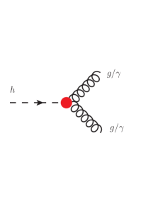
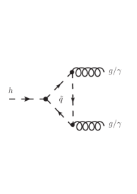
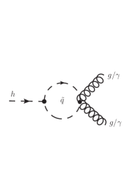
Figure 1: Leading order tree-level Feynman diagram for the EFT (left) and one-loop diagrams for the squark contributions (middle and right) to the $h\to gg/\gamma\gamma$ amplitude.

To estimate quantitatively the validity of the dimension-6 EFT we compare the coefficients obtained above with results from an exact one-loop calculation in the MSSM. This is achieved by calculating the Feynman diagrams in Fig. 1 then matching the $h\to gg$ and $h\to\gamma\gamma$ amplitudes in the EFT with the equivalent MSSM amplitude. In the EFT the operators $\mathcal{O}_{g}$ and $\mathcal{O}_{\gamma}$ can be expanded after electroweak symmetry breaking (EWSB) around the vacuum expectation value $v\sim 174$ GeV in order to get the Lagrangian

$$\mathcal{L}_{hVV}=g_{3}^{2}\sqrt{2}v\frac{\bar{c}_{g}}{m_{W}^{2}}hG^{a}_{\mu\nu}G^{a,\mu\nu}+g_{1}^{2}\sqrt{2}v\frac{\bar{c}_{\gamma}}{m_{W}^{2}}hB_{\mu\nu}B^{\mu\nu}\,,$$

corresponding to the following Feynman rules for the $hgg$ and $h\gamma\gamma$ vertices:

$$iV_{hgg}^{\mu\nu}(p_{2},p_{3}) =-4ig_{3}^{2}\sqrt{2}v\frac{\bar{c}_{g}}{m_{W}^{2}}\big{(}p_{2}p_{3}g^{\mu\nu}-p_{2}^{\nu}p_{3}^{\mu}\big{)}\,,$$

$$iV_{h\gamma\gamma}^{\mu\nu}(p_{2},p_{3}) =-4ie^{2}\sqrt{2}v\frac{\bar{c}_{\gamma}}{m_{W}^{2}}\big{(}p_{2}p_{3}g^{\mu\nu}-p_{2}^{\nu}p_{3}^{\mu}\big{)}\,.$$

Thus the $h\to gg$ and $h\to\gamma\gamma$ amplitudes for on-shell external particles are

$${\cal A}_{EFT}^{hgg} =-16g_{s}^{2}\sqrt{2}v\frac{\bar{c}_{g}}{m_{W}^{2}}\left(\xi_{2}^{*}.\xi_{3}^{*}M_{h}^{2}-2(\xi_{2}^{*}.p_{1})(\xi_{3}^{*}.p_{1})\right)\,,$$ (3.1)

$${\cal A}_{EFT}^{h\gamma\gamma} =-2g_{1}^{2}\cos^{2}\theta_{W}\sqrt{2}v\frac{\bar{c}_{\gamma}}{m_{W}^{2}}\left(\xi_{2}^{*}.\xi_{3}^{*}M_{h}^{2}-2(\xi_{2}^{*}.p_{1})(\xi_{3}^{*}.p_{1})\right)\,,$$ (3.2)

where the $\xi_{i}$ are the polarization vectors of the gauge bosons.

We computed the one-loop diagrams in Fig. 1 in the MSSM and checked our results using the FeynArts package [27]. The CP-even Higgs bosons are rotated to their physical basis by a mixing angle $\alpha$ which we set to be $\alpha=\beta-\pi/2$ corresponding to the decoupling limit when the pseudo-scalar Higgs mass is much heavier than the mass of the Z gauge boson, as indicated by the experimental data [25] and appropriate to our scenario of light stops .

When comparing the EFT and MSSM amplitudes we may choose the momenta of the external particles to be on-shell for convenience. The result of this procedure for the $h\to gg$ amplitude yields the same expression as (3.1) with the replacement $\bar{c}_{g}\to\bar{c}^{\text{MSSM}}_{g}$, where

$$\bar{c}^{\text{MSSM}}_{g}=(\bar{c}^{\text{MSSM}}_{g})^{\tilde{t}}+(\bar{c}^{\text{MSSM}}_{g})^{\tilde{b}}\,,$$ (3.3)

where the part due to stops is given by

$$\quad\quad(\bar{c}^{\text{MSSM}}_{g})^{\tilde{t}}=\frac{m_{W}^{2}}{6(4\pi)^{2}}\frac{N^{\tilde{t}}_{g}}{D^{\tilde{t}}_{g}}\,,$$

$$N^{\tilde{t}}_{g}=\frac{c_{2\beta}g_{1}^{2}}{s^{2}_{W}}\left[v^{2}c_{2\beta}g_{1}^{2}\left(2c_{2W}+1\right)+3\left(3v^{2}h_{t}^{2}+2\left(m_{\tilde{t}_{R}}^{2}-m_{\tilde{Q}}^{2}\right)c_{2W}+2m_{\tilde{Q}}^{2}+m_{\tilde{t}_{R}}^{2}\right)\right]$$

$$\quad\quad+36h_{t}^{2}\left(v^{2}h_{t}^{2}+m_{\tilde{Q}}^{2}+m_{\tilde{t}_{R}}^{2}-X_{t}^{2}\right)\,,$$

$$D^{\tilde{t}}_{g}=\frac{v^{2}c_{2\beta}g_{1}^{2}}{s^{2}_{W}}\left[v^{2}c_{2\beta}g_{1}^{2}\left(2c_{2W}+1\right)+3\left(3v^{2}h_{t}^{2}+4\left(m_{\tilde{t}_{R}}^{2}-m_{\tilde{Q}}^{2}\right)c_{2W}+4m_{\tilde{Q}}^{2}+2m_{\tilde{t}_{R}}^{2}\right)\right]$$

$$\quad\quad+36\left(v^{2}h_{t}^{2}+2m_{\tilde{Q}}^{2}\right)\left(v^{2}h_{t}^{2}+2m_{\tilde{t}_{R}}^{2}\right)-72v^{2}h_{t}^{2}X_{t}^{2}\,,$$

and the sbottom contribution reads,

$$(\bar{c}^{\text{MSSM}}_{g})^{\tilde{b}}=\frac{m_{W}^{2}}{6(4\pi)^{2}}\frac{c_{2\beta}g_{1}^{2}\left\{6\left[\left(m_{\tilde{b}_{R}}^{2}-m_{\tilde{Q}}^{2}\right)c_{2W}+m_{\tilde{Q}}^{2}+2m_{\tilde{b}_{R}}^{2}\right]-v^{2}c_{2\beta}g_{1}^{2}\left(c_{2W}+2\right)\right\}}{\left(12m_{\tilde{b}_{R}}^{2}-v^{2}c_{2\beta}g_{1}^{2}\right)\left[v^{2}c_{2\beta}g_{1}^{2}\left(c_{2W}+2\right)-24m_{\tilde{Q}}^{2}s^{2}_{W}\right]}\,.$$

For $\bar{c}_{\gamma}$ we simply have

$$\bar{c}^{\text{MSSM}}_{\gamma}=\frac{8}{3}(\bar{c}^{\text{MSSM}}_{g})^{\tilde{t}}+\frac{3}{2}(\bar{c}^{\text{MSSM}}_{g})^{\tilde{b}}\,.$$ (3.4)

In the limit $v\to 0$ we obtain the same expressions as $\bar{c}_{g}$ and $\bar{c}_{\gamma}$ in (2.4) and (2.7), respectively. Since $\bar{c}_{g}$ and $\bar{c}_{\gamma}$ correspond to a truncation of the full theory at the dimension-6 level, they contain only the leading-order terms in an expansion in inverse powers of the stop mass, whereas the MSSM result is exact and include higher-order terms in $v/m_{\tilde{t},\tilde{b}}$ that would be generated by higher-dimensional operators in the EFT approach. Therefore, we expect the discrepancy between the two approaches to scale with the ratio $v/m_{\tilde{t},\tilde{b}}$ for $m_{\tilde{t},\tilde{b}}$, and the differences between the EFT and exact MSSM results gives insight into the potential importance of such higher-dimensional operators. We note that a large value of $X_{t}$ in terms like $v^{2}m_{W}^{2}X_{t}^{2}/m^{6}_{\tilde{t}}$ could potentially affect the validity of the EFT even for large stop masses, but the positivity of the lightest physical mass eigenvalue imposes an upper limit $X_{t}\simeq m_{\tilde{t}}^{2}/m_{t}$.

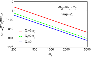
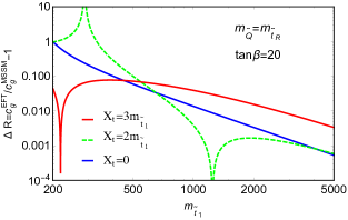
Figure 2: Values of $\Delta R$, defined in (3.13), in the degenerate case $m_{\tilde{Q}}=m_{\tilde{t}_{R}}\equiv m_{\tilde{t}}$ for $\tan\beta=20$ and the indicated values of $X_{t}$, as a function of $m_{\tilde{t}}$ (left panel), and as functions of $m_{\tilde{t}_{1}}$ (right panel).

The physical mass eigenstates are obtained by diagonalizing the squark mass matrices [24]

$${\cal M}^{2}_{\tilde{q}}=\left(\begin{array}[]{cc}m_{q}^{2}+m_{LL}^{2}&m_{q}\,X_{q}\\ m_{q}\,X_{q}&m_{q}^{2}+m_{RR}^{2}\end{array}\right)$$ (3.7)

with the various entries defined by

$$m_{LL}^{2} =m_{\tilde{Q}}^{2}+(I^{3L}_{q}-Q_{q}s_{W}^{2})\,M_{Z}^{2}\,c_{2\beta}\,,$$ (3.8)

$$m_{RR}^{2} =m_{\tilde{q}_{R}}^{2}+Q_{q}s_{W}^{2}\,M_{Z}^{2}\,c_{2\beta}\,,$$ (3.9)

$$X_{q} =A_{q}-\mu(\tan\beta)^{-2I_{q}^{3L}}\,.$$ (3.10)

$Q_{q}$ and $I^{3L}_{q}$ is the electromagnetic charge and the weak doublet isospin respectively. After rotating the $2\times 2$ matrices by an angle $\theta_{q}$, which transforms the interaction eigenstates $\tilde{q}_{L}$ and $\tilde{q}_{R}$ into the mass eigenstates $\tilde{q}_{1}$ and $\tilde{q}_{2}$, the mixing angle and physical squark masses are given by

$$s_{2\theta_{q}}=\frac{2m_{q}X_{q}}{m_{\tilde{q}_{1}}^{2}-m_{\tilde{q}_{2}}^{2}}\ \ ,\ \ c_{2\theta_{q}}=\frac{m_{LL}^{2}-m_{RR}^{2}}{m_{\tilde{q}_{1}}^{2}-m_{\tilde{q}_{2}}^{2}}\hskip 51.21504pt$$ (3.11)

$$m_{\tilde{q}_{1,2}}^{2}=m_{q}^{2}+\frac{1}{2}\left[m_{LL}^{2}+m_{RR}^{2}\mp\sqrt{(m_{LL}^{2}-m_{RR}^{2})^{2}+4m_{q}^{2}X_{q}^{2}}\ \right]\,.$$ (3.12)

We see that in the stop sector the mixing is strong for large values of the parameter $X_{t}=A_{t}-\mu\cot\beta$, which generates a large mass splitting between the two physical mass eigenstates and makes $\tilde{q}_{1}$ much lighter than the other sparticle $\tilde{q}_{2}$.

We now compare the values of the $\bar{c}_{g}$ coefficients calculated in the MSSM and the EFT :

$$\Delta R\;\equiv\;\frac{\bar{c}^{\text{EFT}}_{g}}{\bar{c}^{\text{MSSM}}_{g}}-1\,.$$ (3.13)

Fig. 2 displays values of $\Delta R$ for the degenerate case $m_{\tilde{Q}}=m_{\tilde{t}_{R}}\equiv m_{\tilde{t}}$, three different values of $X_{t}$ and the representative choice $\tan\beta=20$. In the left panel we plot $\Delta R$ as functions of $m_{\tilde{t}}$, and the right panel shows $\Delta R$ as functions of the lighter stop mass, $m_{\tilde{t}_{1}}$. We see that in both cases $\Delta R\lesssim 0.1$ for $m_{\tilde{t}}(m_{\tilde{t}_{1}})\gtrsim 500$ GeV, with a couple of exceptions. One is for the relatively large value $X_{t}=3m_{\tilde{t}}$ in the left panel, for which $\Delta R\gtrsim 0.1$ for $m_{\tilde{t}}\lesssim 1000$ GeV, and the other is for $X_{t}=2m_{\tilde{t}_{1}}$ and $m_{\tilde{t}_{1}}\sim 290$ GeV in the right panel, which is due to a node in $\bar{c}^{\text{MSSM}}_{g}$. These results serve as a warning that, although the EFT approach is in general quite reliable for stop mass parameters $\gtrsim 500$ GeV, care should always be exercised for masses $\lesssim 1000$ GeV.

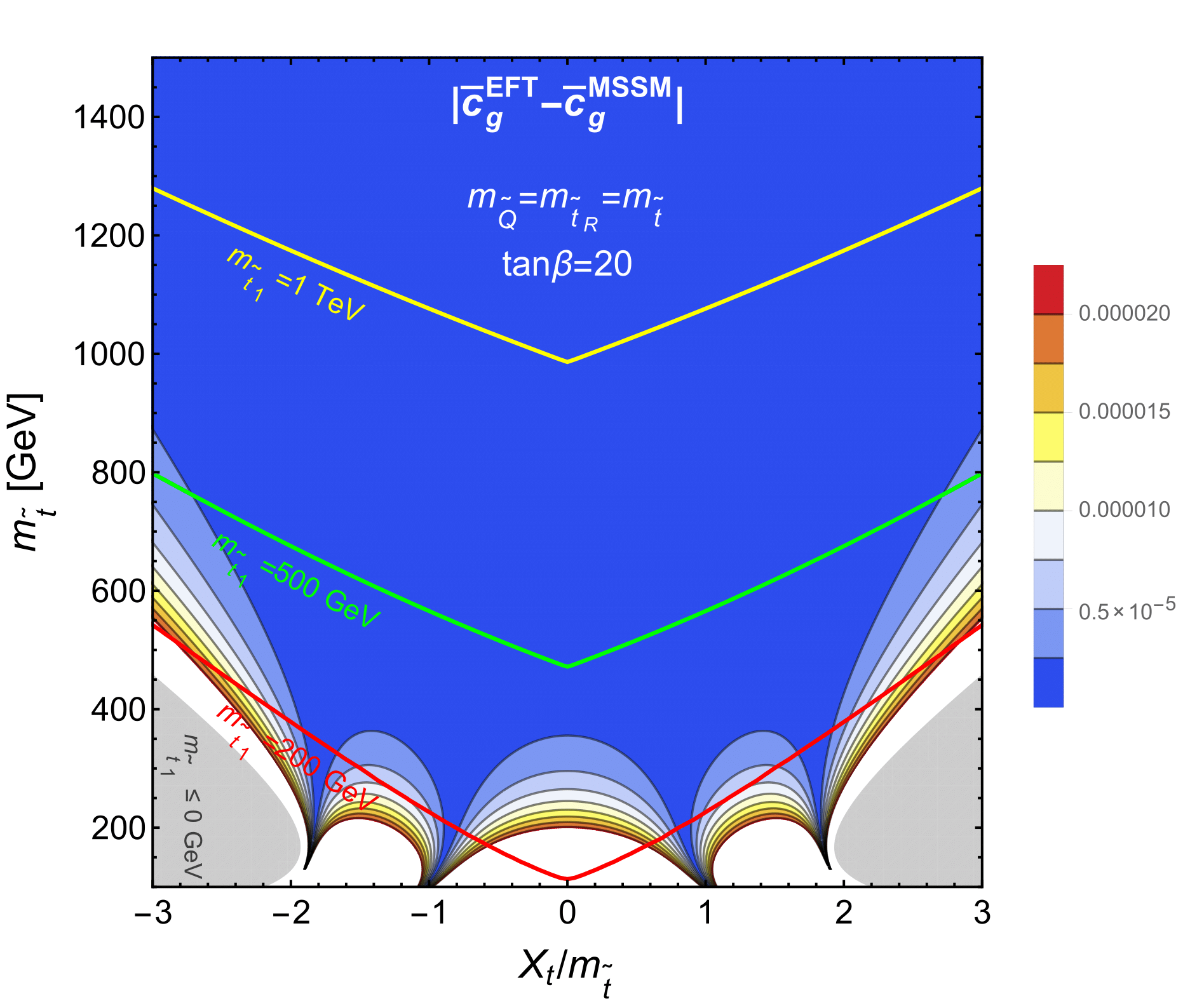
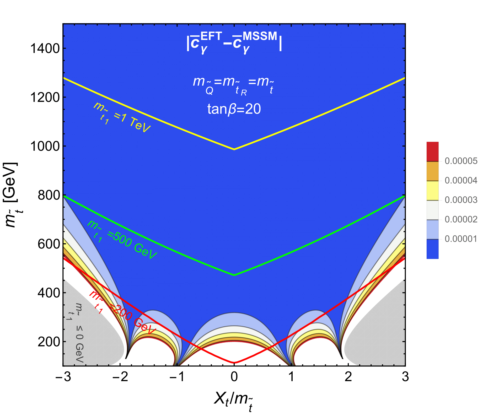
Figure 3: Contours of the differences $|\bar{c}_{g}^{\rm EFT}-\bar{c}_{g}^{\rm MSSM}|$ (left panel) and $|\bar{c}_{\gamma}^{\rm EFT}-\bar{c}_{\gamma}^{\rm MSSM}|$ (right panel) in $(X_{t}/m_{\tilde{t}},m_{\tilde{t}})$ planes for the degenerate case $m_{\tilde{Q}}=m_{\tilde{t}_{R}}\equiv m_{\tilde{t}}$ with $\tan\beta=20$. Also shown are contours of $m_{\tilde{t}_{1}}=200$ GeV, $500$ GeV and $1$ TeV and regions where the ${\tilde{t}_{1}}$ becomes tachyonic.

A similar message is conveyed by Fig. 3, which uses colour-coding to display values of the differences $|\bar{c}_{g}^{\rm EFT}-\bar{c}_{g}^{\rm MSSM}|$ (left panel) and $|\bar{c}_{\gamma}^{\rm EFT}-\bar{c}_{\gamma}^{\rm MSSM}|$ (right panel) in $(X_{t}/m_{\tilde{t}},m_{\tilde{t}})$ planes for the degenerate case $m_{\tilde{Q}}=m_{\tilde{t}_{R}}\equiv m_{\tilde{t}}$ with $\tan\beta=20$. Also shown are contours of $m_{\tilde{t}_{1}}=200$ GeV (red), 500 GeV (green) and 1 TeV (yellow) and regions where the ${\tilde{t}_{1}}$ becomes tachyonic (shaded grey). We see that the differences are generally $<2.5\times 10^{-6}$ for $|\bar{c}_{g}^{\rm EFT}-\bar{c}_{g}^{\rm MSSM}|$ and $<10^{-5}$ for $|\bar{c}_{\gamma}^{\rm EFT}-\bar{c}_{\gamma}^{\rm MSSM}|$ when $m_{\tilde{t}_{1}}>500$ GeV, even for large values of $X_{t}$, but that much larger differences are possible for $m_{\tilde{t}_{1}}<200$ GeV, even for small values of $X_{t}$.

4 Constraints on Light Stops from a Global Fit

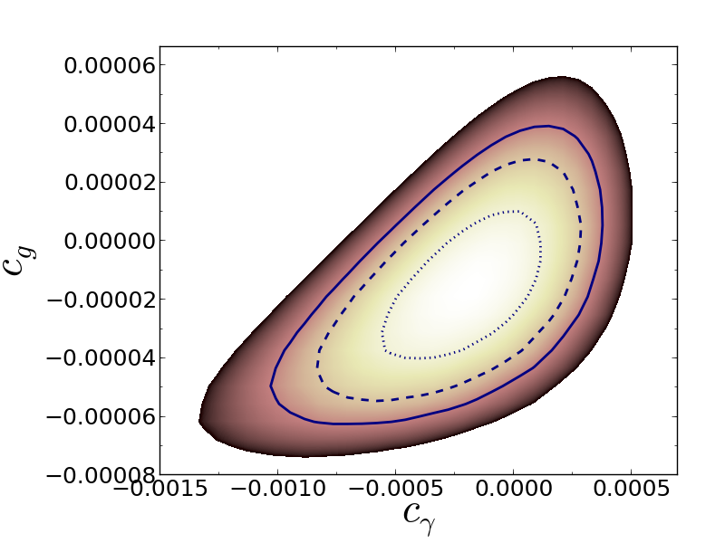
Figure 4: Results based on the global fit in [6], varying $\bar{c}_{g}$ and $\bar{c}_{\gamma}$ simultaneously but setting to zero the coefficients of the other dimension-6 operators contributing to the Higgs sector. The dotted, dashed and solid contours on the left denote the allowed 68%, 95% and 99% CL regions respectively. The middle and right figures show the marginalized $\chi^{2}$ functions for $\bar{c}_{\gamma}$ and $\bar{c}_{g}$ respectively.

We now discuss the constraints on the lighter stop mass that are imposed by the current experimental constraints on the coefficients $\bar{c}_{g}$ and $\bar{c}_{\gamma}$, comparing them with the constraints imposed by electroweak precision observables via the oblique parameters $S$ and $T$ [31], as well as the ranges favoured by measurements of the Higgs mass $M_{h}$ and direct searches at the LHC. We note that the $S$ and $T$ parameters are related to the dimension-6 operator coefficients $\bar{c}_{W}$, $\bar{c}_{B}$ and $\bar{c}_{T}$, as defined in the basis of [6] , through

$$S =\frac{4\sin^{2}{\theta_{W}}}{\alpha(m_{Z})}(\bar{c}_{W}+\bar{c}_{B})\approx 119(\bar{c}_{W}+\bar{c}_{B})\,,$$

$$T =\frac{1}{\alpha(m_{Z})}\bar{c}_{T}\approx 129\bar{c}_{T}\,.$$

We shall quote the electroweak precision constraints on $\bar{c}_{W}+\bar{c}_{B}$ and $\bar{c}_{T}$ instead of $S$ and $T$, in keeping with the EFT approach. The stop contributions to these coefficients were given in [12, 13], and Table 1 displays the current experimental constraints on $\bar{c}_{g},\bar{c}_{\gamma},\bar{c}_{T}$ and $\bar{c}_{W}+\bar{c}_{B}$ that we apply.

Coeff.	Experimental constraints		95 % CL limit	deg. $m_{\tilde{t}_{1}}$,
				$X_{t}=0$
$\bar{c}_{g}$	LHC	marginalized	$[-4.5,2.2]\times 10^{-5}$	$\sim 410$ GeV
		individual	$[-3.0,2.5]\times 10^{-5}$	$\sim 390$ GeV
$\bar{c}_{\gamma}$	LHC	marginalized	$[-6.5,2.7]\times 10^{-4}$	$\sim 215$ GeV
		individual	$[-4.0,2.3]\times 10^{-4}$	$\sim 230$ GeV
$\bar{c}_{T}$	LEP	marginalized	$[-10,10]\times 10^{-4}$	$\sim 290$ GeV
		individual	$[-5,5]\times 10^{-4}$	$\sim 380$ GeV
$\bar{c}_{W}+\bar{c}_{B}$	LEP	marginalized	$[-7,7]\times 10^{-4}$	$\sim 185$ GeV
		individual	$[-5,5]\times 10^{-4}$	$\sim 195$ GeV

Table 1: List of the experimental $95\%$ CL bounds on coefficients used in setting current limits on stops, which are taken from [6]. The marginalized LHC limits are for a two-parameter fit allowing $\bar{c}_{g}$ and $\bar{c}_{\gamma}$ to vary, and the marginalized LEP limits are for a two-parameter fit of $\bar{c}_{T}$ and $\bar{c}_{W}+\bar{c}_{B}$. The corresponding lightest stop mass limits shown are for degenerate soft-supersymmetry breaking masses $m_{\tilde{Q}}=m_{\tilde{t}_{R}}=m_{\tilde{t}}$ with $X_{t}=0$.

The constraints on the coefficients in the penultimate column of Table 1 are taken from a recent global analysis [6] of LEP, LHC and Tevatron data on Higgs production and triple-gauge couplings. For $\bar{c}_{g}$ and $\bar{c}_{\gamma}$ we list the current 95% CL ranges after marginalising a two-parameter fit in which both $\bar{c}_{g}$ and $\bar{c}_{\gamma}$ are allowed to vary , as well as considering the more restrictive ranges found when only $\bar{c}_{g}$ or $\bar{c}_{\gamma}\neq 0$ individually, with the other operator coefficients set to zero. Similar marginalized and individual 95% CL limits on $\bar{c}_{T}$ and $\bar{c}_{W}+\bar{c}_{B}$ are displayed, where the two-parameter fit varying $\bar{c}_{T}$ and $\bar{c}_{W}+\bar{c}_{B}$ simultaneously is equivalent to the $S,T$ ellipse, as reproduced in [6]. We note that the stop contributions to the coefficients of the other relevant operators are far smaller than the ranges of these coefficients that were found in the global fit. This indicates that one is justified in setting these other operator coefficients to zero when considering bounds on the stop sector, if one assumes that there are no important contributions from other possible new physics.

4.1 Degenerate Stop Masses

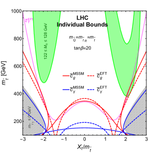
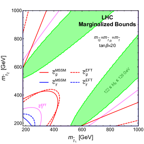
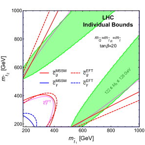
Figure 5: Compilation of the constraints in (upper panels) the $(X_{t}/m_{\tilde{t}_{1}},m_{\tilde{t}})$ plane and (lower panels) the $(m_{\tilde{t}},m_{\tilde{t}_{2}})$ plane from (left panels) the marginalized bounds on $\bar{c}_{g}$ (red lines) and $\bar{c}_{\gamma}$ (blue lines), and from (right panels) the individual bounds on $\bar{c}_{g}$ and $\bar{c}_{\gamma}$. Also shown are the EFT bounds on $\bar{c}_{T}$ (purple lines), the constraint that the lighter stop should not be tachyonic (grey shading) and the region where $M_{h}\in(122,128)$ GeV according to a FeynHiggs 2.10.3 [29] calculation assuming no other significant contributions from outside the stop sector (green shading).

Fig. 5 displays the current constraints in the case of degenerate soft masses $m_{\tilde{Q}}=m_{\tilde{t}_{R}}\equiv m_{\tilde{t}}$ with decoupled sbottoms, in the upper panels for $m_{\tilde{t}}$ as functions of $X_{t}/m_{\tilde{t}}$ and in the lower panels for $m_{\tilde{t}_{2}}$ as functions of $m_{\tilde{t}_{1}}$, in both cases for $\tan\beta=20$. The left panels show the stop constraints from the current marginalized 95% bounds on $\bar{c}_{g}$ (red lines) and $\bar{c}_{\gamma}$ (blue lines), and the right panels show the corresponding bounds from the current marginalized 95% bounds. The solid (dashed) lines are obtained from an exact one-loop MSSM analysis and the EFT approach, respectively. The purple lines show the individual bound from $\bar{c}_{T}$ in the EFT approach. The bounds from $\bar{c}_{W}+\bar{c}_{B}$ corresponding to the $S$ parameter are negligible and omitted here. The grey shaded regions are excluded because the lighter stop becomes tachyonic, and the green shaded regions correspond to 122 GeV$<M_{h}<$128 GeV, as calculated using FeynHiggs 2.10.3 [29], allowing for a theoretical uncertainty of $\pm 3$ GeV and assuming that there are no other important MSSM contributions to $M_{h}$.

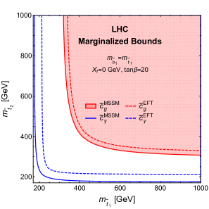
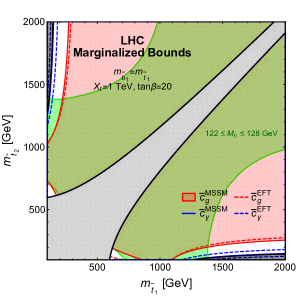
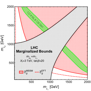
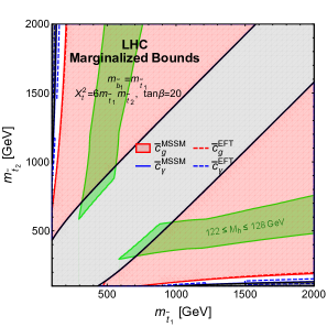
Figure 6: Compilation of the constraints in the case of non-degenerate soft mass parameters, including also sbottom squarks and assuming $m_{\tilde{b}_{1}}=m_{\tilde{t}_{1}}$ under the hypotheses $\tan\beta=20$ and $X_{t}=0$ (upper left panel), $X_{t}=1$ TeV (upper right panel), $X_{t}=3$ TeV (lower left panel) and $X_{t}=\sqrt{6m_{\tilde{t}_{1}}m_{\tilde{t}_{2}}}$ (lower right panel). The red (blue) lines show the current individual 95% CL constraints from $\bar{c}_{g}$ ($\bar{c}_{\gamma}$) as evaluated exactly in the MSSM (solid lines) and in the EFT approach. Additionally, the region compatible with $\bar{c}_{g}$ is shaded pink, the band compatible with $M_{h}$ is shaded green, and regions disallowed by the mixing hypothesis or the appearance of a tachyonic stop are shaded grey.

We see in the upper panels of Fig. 5 that the $\bar{c}_{g}$ constraints on $m_{\tilde{t}_{1}}$ are generally the strongest, except for large $|X_{t}/m_{\tilde{t}}|$. We also observe that the MSSM and EFT evaluations give rather similar bounds on $m_{\tilde{t}_{1}}$ for $|X_{t}/m_{\tilde{t}}|\lesssim 1$ and $\gtrsim 2$. However, there are significant differences for $1\lesssim|X_{t}/m_{\tilde{t}}|\lesssim 2$, due to the fact that the two evaluations have zeroes at different values of $X_{t}/m_{\tilde{t}}$. The next most sensitive constraints are those from $T$, parametrised here by the coefficient $\bar{c}_{T}$, which become competitive with the $\bar{c}_{g}$ constraints at large $|X_{t}/m_{\tilde{t}}|$, but are significantly weaker for small values of $X_{t}/m_{\tilde{t}}$. The constraints from $\bar{c}_{\gamma}$ are weaker still for all values of $X_{t}/m_{\tilde{t}}$, as might have been expected because the global fit in [6] gave constraints on $\bar{c}_{\gamma}$ that are weaker than those on $\bar{c}_{g}$. Indeed, the $\bar{c}_{\gamma}$ constraint is not significantly stronger than the constraint that the ${\tilde{t}_{1}}$ not be tachyonic, as shown by the grey shading in the upper panels of Fig. 5. We also note that the LHC measurement of $M_{h}$ favours $|X_{t}/m_{\tilde{t}}|\gtrsim 2$ and values of $m_{\tilde{t}}$ that are consistent with the EFT bounds.

These results are reflected in the lower panels of Fig. 5, where we present the $(m_{\tilde{t}_{1}},m_{\tilde{t}_{2}})$ planes with the marginalized constraints (left panel) and the individual constraints (right panel). The MSSM and EFT implementations of the $\bar{c}_{g}$ constraint give qualitatively similar results, and (except for extreme values of $m_{\tilde{t}_{1}}/m_{\tilde{t}_{2}}$) are generally stronger than the constraints from $\bar{c}_{T}$, which are in turn stronger than the $\bar{c}_{\gamma}$ constraint. We also note that the LHC measurement of $M_{h}$ favours moderate values of $m_{\tilde{t}_{1}}/m_{\tilde{t}_{2}}$ and values of $m_{\tilde{t}_{1}}$ or $m_{\tilde{t}_{2}}\gtrsim 520$ GeV.

The limits on the lightest stop mass for degenerate soft-supersymmetry breaking masses $m_{\tilde{Q}}=m_{\tilde{t}_{R}}=m_{\tilde{t}}$ with $X_{t}=0$ are shown in the last column of Table 1.

4.2 Non-Degenerate Stop Masses

We consider now cases with non-degenerate stop soft mass parameters, allowing also for the possibility that the lighter sbottom squark plays a rôle. We show in Fig. 6 various planes under the hypotheses $m_{\tilde{b}_{1}}=m_{\tilde{t}_{1}}$ and $\tan\beta=20$, considering several possibilities for $X_{t}$. In all panels, the constraints from the individual 95% bound on $\bar{c}_{g}$ are indicated by red lines and those from $\bar{c}_{\gamma}$ are indicated by blue lines (solid for the exact MSSM evaluation and dashed for the EFT approach), and the region allowed by the exact calculation is shaded pink.

The upper left panel is for $X_{t}=0$: we see that in the limit $m_{\tilde{t}_{2}}\gg m_{\tilde{t}_{1}}$ the $\bar{c}_{g}$ constraint imposes $m_{\tilde{t}_{1}}\gtrsim 300$ GeV, with a difference of $\sim 20$ GeV between the exact and EFT calculations. On the other hand, if $m_{\tilde{t}_{2}}=m_{\tilde{t}_{1}}$ we find $m_{\tilde{t}_{1}}\gtrsim 380$ GeV, again with the EFT calculation giving a bound $\sim 20$ GeV stronger than the exact MSSM calculation. The corresponding bounds from the individual 95% constraint on $\bar{c}_{\gamma}$ are $\simeq 100$ GeV weaker. However, we note that the LHC constraint on $M_{h}$ is not respected anywhere in this plane.

Turning now to the case $X_{t}=1$ TeV shown in the upper right panel of Fig. 6, we see a grey shaded band around the $m_{\tilde{t}_{1}}=m_{\tilde{t}_{2}}$ line that is disallowed by ${\tilde{t}_{1}}-{\tilde{t}_{2}}$ mixing, and other grey shaded regions where $m_{\tilde{t}_{1}}\ll m_{\tilde{t}_{2}}$ (or vice versa) and the lighter stop is tachyonic. In this case the $M_{h}$ constraint (green shaded band) can be satisfied, with small strips of the parameter space ruled out by the $\bar{c}_{g}$ constraint. The $\bar{c}_{\gamma}$ constraint is unimportant in this case.

When $X_{t}$ is increased to 3 TeV, as shown in the lower left panel of Fig. 6, the diagonal band forbidden by mixing expands considerably, and the $\bar{c}_{\gamma}$ constraint disappears. In this case the $\bar{c}_{g}$ constraint would allow $(m_{\tilde{t}_{1}},m_{\tilde{t}_{2}})\gtrsim(400,1100)$ GeV on the boundary of the band forbidden by the mixing hypothesis, but the $M_{h}$ constraint is stronger, enforcing $(m_{\tilde{t}_{1}},m_{\tilde{t}_{2}})\gtrsim(800,1300)$ GeV along this boundary.

Finally, we consider in the lower right panel of Fig. 6 the so-called maximal-mixing hypothesis $X_{t}=\sqrt{6m_{\tilde{t}_{1}}m_{\tilde{t}_{2}}}$. In this case, almost the entire $(m_{\tilde{t}_{1}},m_{\tilde{t}_{2}})$ plane is allowed by the $\bar{c}_{g}$ constraint, whereas a triangular region at small $m_{\tilde{t}_{1}}$ and/or $m_{\tilde{t}_{2}}$ is forbidden by the $M_{h}$ constraint.

It is interesting to compare the limits on $m_{\tilde{t}_{1}}$ that we find with those found in a recent global fit to the pMSSM [30] in which universal third-generation squark masses were assumed at the renormalisation scale $\sqrt{m_{\tilde{t}_{1}}m_{\tilde{t}_{2}}}$, the first- and second-generation squark masses were assumed to be equal, but allowed to differ from the third-generation mass as were the slepton masses, arbitrary non-universal gaugino masses $M_{1,2,3}$ were allowed, and the trilinear soft supersymmetry-breaking parameter $A$ was assumed to be universal but otherwise free. That analysis included LHC, dark matter and flavour constraints, as well as electroweak precision observables and Higgs measurements, and found $m_{\tilde{t}_{1}}\gtrsim 400$ GeV. The analysis of this paper uses somewhat different assumptions and hence is not directly comparable, but it is interesting that the one-loop sensitivity of $\bar{c}_{g}$ to the stop mass parameters is quite comparable.

5 Sensitivities of Possible Future Precision Measurements

Coeff.	Experimental constraints		95 % CL limit	deg. $m_{\tilde{t}_{1}}$
				$X_{t}=0$	$X_{t}=m_{\tilde{t}}/2$
$\bar{c}_{g}$	$\text{ILC}_{250\text{GeV}}^{1150\text{fb}^{-1}}$	marginalized	$[-7.7,7.7]\times 10^{-6}$	$\sim 675$ GeV	$\sim 520$ GeV
		individual	$[-7.5,7.5]\times 10^{-6}$	$\sim 680$ GeV	$\sim 545$ GeV
	FCC-ee	marginalized	$[-3.0,3.0]\times 10^{-6}$	$\sim 1065$ GeV	$\sim 920$ GeV
		individual	$[-3.0,3.0]\times 10^{-6}$	$\sim 1065$ GeV	$\sim 915$ GeV
$\bar{c}_{\gamma}$	$\text{ILC}_{250\text{GeV}}^{1150\text{fb}^{-1}}$	marginalized	$[-3.4,3.4]\times 10^{-4}$	$\sim 200$ GeV	$\sim 40$ GeV
		individual	$[-3.3,3.3]\times 10^{-4}$	$\sim 200$ GeV	$\sim 35$ GeV
	FCC-ee	marginalized	$[-6.4,6.4]\times 10^{-5}$	$\sim 385$ GeV	$\sim 250$ GeV
		individual	$[-6.3,6.3]\times 10^{-5}$	$\sim 390$ GeV	$\sim 260$ GeV
$\bar{c}_{T}$	$\text{ILC}_{250\text{GeV}}^{1150\text{fb}^{-1}}$	marginalized	$[-3,3]\times 10^{-4}$	$\sim 480$ GeV	$\sim 285$ GeV
		individual	$[-7,7]\times 10^{-5}$	$\sim 930$ GeV	$\sim 780$ GeV
	FCC-ee	marginalized	$[-3,3]\times 10^{-5}$	$\sim 1410$ GeV	$\sim 1285$ GeV
		individual	$[-0.9,0.9]\times 10^{-5}$	$\sim 2555$ GeV	$\sim 2460$ GeV
$\bar{c}_{W}+\bar{c}_{B}$	$\text{ILC}_{250\text{GeV}}^{1150\text{fb}^{-1}}$	marginalized	$[-2,2]\times 10^{-4}$	$\sim 230$ GeV	$\sim 170$ GeV
		individual	$[-6,6]\times 10^{-5}$	$\sim 340$ GeV	$\sim 470$ GeV
	FCC-ee	marginalized	$[-2,2]\times 10^{-5}$	$\sim 545$ GeV	$\sim 960$ GeV
		individual	$[-0.8,0.8]\times 10^{-5}$	$\sim 830$ GeV	$\sim 1590$ GeV

Table 2: List of the $95\%$ CL bounds on EFT operator coefficients from projected constraints on Higgs couplings and electroweak precision observables at the future $e^{+}e^{-}$ colliders ILC and FCC-ee. The marginalized limits on $\bar{c}_{g}$ or $\bar{c}_{\gamma}$ ($\bar{c}_{T}$ or $\bar{c}_{W}+\bar{c}_{B}$) are for a two-parameter fit allowing $\bar{c}_{g}$ and $\bar{c}_{\gamma}$ ($\bar{c}_{T}$ and $\bar{c}_{W}+\bar{c}_{B}$) to vary simultaneously but setting other operator coefficients to zero. The corresponding lightest stop mass limits shown are for degenerate soft-supersymmetry breaking masses $m_{\tilde{Q}}=m_{\tilde{t}_{R}}=m_{\tilde{t}}$ with $X_{t}=0$ and $X_{t}/m_{\tilde{t}}=2$.

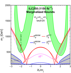
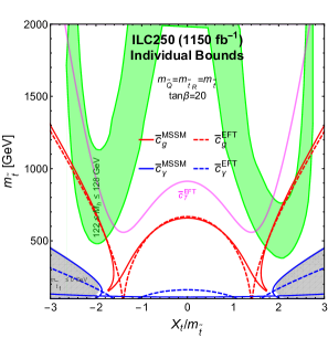
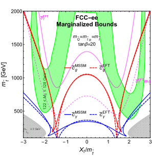
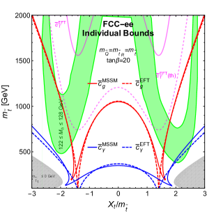
Figure 7: The $(X_{t}/m_{\tilde{t}},m_{\tilde{t}})$ planes, analogous to those in the upper panels of Fig. 5, showing prospective marginalized bounds (left panels) and individual bounds (right panels) from the ILC [33] with $1150~{}\text{fb}^{-1}$ of luminosity at $250$ GeV (upper panels) and from FCC-ee [32] with $10^{4}~{}\text{fb}^{-1}$ of luminosity at $240$ GeV (lower panels). In the latter case, the solid purple lines are the 95% CL contours for electroweak precision measurements from FCC-ee incorporating the projected statistical and systematic experimental errors alone, and the dashed purple lines also include theory errors from [35].

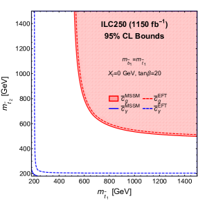
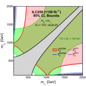
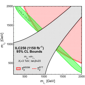
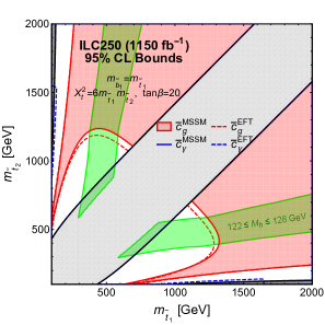
Figure 8: Compilation of projected ILC 95 % CL bounds from $\bar{c}_{g}$ ($\bar{c}_{\gamma}$) given by red (blue) lines in the $m_{\tilde{t}_{1}}$ vs $m_{\tilde{t}_{2}}$ plane, analogous to Fig. 6, with $m_{\tilde{b}_{1}}=m_{\tilde{t}_{1}}$ and $\tan{\beta}=20$. Values of $X_{t}=0,1,3,\sqrt{6m_{\tilde{t}_{1}}m_{\tilde{t}_{2}}}$ TeV are shown clockwise from top left. The marginalized limits are displayed and the individual bounds are very similar.

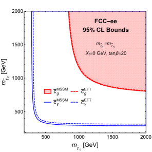
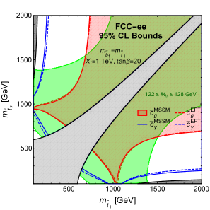
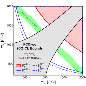
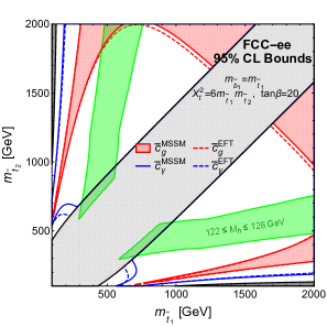
Figure 9: Compilation of projected FCC-ee 95 % CL bounds from $\bar{c}_{g}$ ($\bar{c}_{\gamma}$) given by red (blue) lines in the $m_{\tilde{t}_{1}}$ vs $m_{\tilde{t}_{2}}$ plane, analogous to Fig. 6, with $m_{\tilde{b}_{1}}=m_{\tilde{t}_{1}}$ and $\tan{\beta}=20$. Values of $X_{t}=0,1,3,\sqrt{6m_{\tilde{t}_{1}}m_{\tilde{t}_{2}}}$ TeV is shown clockwise from top left. The marginalized limits are displayed and the individual bounds are very similar.

We saw in the previous Section that the precision of current measurements does not exclude in a model-independent way most of the parameter space for a stop below the TeV scale, and barely reaches into the region required for a 125 GeV Higgs mass in the MSSM. However, future colliders will increase significantly the precision of electroweak and Higgs measurements to the level required to challenge seriously the naturalness paradigm and test the MSSM calculations of $M_{h}$.

In this Section we assess the potential improvements for constraints on a light stop possible with future $e^{+}e^{-}$ colliders. As previously, we perform an analysis in the EFT framework via the corresponding bounds on the relevant dimension-6 coefficients, and compare it with the exact one-loop MSSM calculation. As representative examples of future $e^{+}e^{-}$ colliders, we focus on the ILC [33] and FCC-ee [32] (formerly known as TLEP) proposals. The scenarios considered here for the ILC and FCC-ee postulate centre-of-mass energies of 250 and 240 GeV with luminosities of 1150 $\text{fb}^{-1}$ and 10000 $\text{fb}^{-1}$, respectively.

Table 2 lists the prospective 95% CL limits obtained on $\bar{c}_{g},\bar{c}_{\gamma},\bar{c}_{T},$ and $\bar{c}_{W}+\bar{c}_{B}$ from a $\chi^{2}$ analysis, with the marginalized constraints on $\bar{c}_{g}$ and $\bar{c}_{\gamma}$ obtained in a two-parameter fit to just these coefficients, and similarly for $\bar{c}_{T}$ and $\bar{c}_{W}+\bar{c}_{B}$, corresponding to the $T$ and $S$ parameters respectively, as well as the constraints obtained when each operator coefficient is allowed individually to be non-zero. The target precisions on experimental errors for the electroweak precision observables $m_{W},\Gamma_{Z},R_{l}$ and $A_{l}$ at the ILC are given in [33], and those at FCC-ee were taken from [32], and include important systematic uncertainties. The errors on the Higgs associated production cross-section times branching ratio are from [34] for the ILC and from [22] for FCC-ee. The numbers quoted in Table 2 neglect theoretical uncertainties, in order to reflect the possible performances of the experiments . The treatment of the dimension-6 coefficients in the observables follows a procedure similar to that of the global fit performed in [6], and we use the results of [14] to rescale the constraint from associated Higgs production.

5.1 Degenerate Stop Masses

Contours from possible future constraints on $\bar{c}_{g}$, $\bar{c}_{\gamma}$ and $\bar{c}_{T}$ for the case of degenerate soft masses $m_{\tilde{Q}}=m_{\tilde{t}_{R}}\equiv m_{\tilde{t}}$ are plotted in Fig. 7, using again the value $\tan{\beta}=20$. The upper panels show results for the ILC, the lower panels for FCC-ee, the left panels show the marginalized constraints and the right panels show the individual constraints. The grey and green shaded regions are the same as in Fig. 7. We see that the marginal and individual sensitivities to $m_{\tilde{t}}$ from $\bar{c}_{g}$ and $\bar{c}_{\gamma}$ are very similar, whereas the individual sensitivity of $\bar{c}_{T}$ are much stronger, particularly at FCC-ee. We see that ILC is indirectly sensitive to $m_{\tilde{t}}\sim 600$ GeV, and that FCC-ee is indirectly sensitive to stops in the TeV range. The measurement of the $\bar{c}_{T}$ coefficient at FCC-ee has the highest potential reach, though this will be highly dependent on future improvements in reducing theory uncertainties [22, 35].

The limits on the lightest stop mass for degenerate soft-supersymmetry breaking masses $m_{\tilde{Q}}=m_{\tilde{t}_{R}}=m_{\tilde{t}}$ with $X_{t}=0$ and $X_{t}/m_{\tilde{t}}=2$ are shown in the two last columns of Table 2.

5.2 Non-Degenerate Stop Masses

Moving on to the non-degenerate case, the $\bar{c}_{g}$ and $\bar{c}_{\gamma}$ 95% CL limits for ILC and FCC-ee are plotted in the $m_{\tilde{t}_{1}}$ vs $m_{\tilde{t}_{2}}$ plane for various $X_{t}$ values in Fig. 8 and 9 respectively. The top left, top right, and bottom left plots correspond to $X_{t}=0,1$ and 3 TeV respectively, while the bottom right plot is for the maximal-mixing hypothesis $X_{t}=\sqrt{6m_{\tilde{t}_{1}}m_{\tilde{t}_{2}}}$. We see that the ILC sensitivity to $\bar{c}_{g}$ begins to probe and potentially exclude parts of the green shaded region compatible with the measured $M_{h}$, while FCC-ee would push the sensitivity of $\bar{c}_{g}$ constraints into the TeV scale. In particular, it could eliminate the entire allowed $M_{h}$ region for $X_{t}=3$ TeV.

6 Conclusions and Prospects

In light of the SM-like Higgs sector and the current lack of direct evidence for additional degrees of freedom beyond the SM, the framework of the Effective SM (ESM) is gaining increasing attention as a general framework for characterising the indirect effects of possible new physics in a model-independent way. The ESM is simply the SM extended in the way it has always been regarded: as an effective field theory supplemented by higher-dimensional operators suppressed by the scale of new physics. The leading lepton-number-conserving effects are parametrised by dimension-6 operators, whose coefficients are determined by matching to a UV model and constrained through their effects on experimental observables. In this paper we have illustrated all these steps in the EFT approach for light stops in the MSSM.

In particular, we employed the CDE method to compute the one-loop effective Lagrangian, showing how certain results derived previously under the assumption of a degenerate mass matrix can be generalised to the non-degenerate case. The universal one-loop effective Lagrangian can then be used without caveats to obtain directly one-loop Wilson coefficients. The advantage of this was demonstrated here in the calculation of the $\bar{c}_{g}$ and $\bar{c}_{\gamma}$ coefficients. One simply takes the mass and $U$ matrices from the quadratic term of the heavy field being integrated out, as defined in (2.1), and substitutes it with the corresponding field strength matrix into the universal expression obtained from the CDE expansion [23] to get the desired operators, without having to evaluate any loop integrals or match separate calculations in the UV and EFT.

Since the $hgg$ and $h\gamma\gamma$ couplings are loop-induced in the SM, the $\bar{c}_{g}$ and $\bar{c}_{\gamma}$ coefficients are currently the most sensitive to light stops. The stop contribution to these coefficients is also loop-suppressed, thus lowering the EFT cut-off scale, and it is natural to ask at what point the EFT breaks down and the effects of higher-dimensional operators are no longer negligible. We addressed this question by comparing the EFT coefficients with a full calculation in the MSSM, finding that the disagreement is generally $\lesssim 10\%$ for a lightest stop mass $m_{\tilde{t}_{1}}\gtrsim 500$ GeV, with the exception of a large $|X_{t}|\geq 3m_{\tilde{t}_{1}}$ or accidental cancellations in the Higgs-stop couplings.

The constraints on $\bar{c}_{g}$ and $\bar{c}_{\gamma}$ from a global fit to the current LHC and Tevatron data, and the constraints on $\bar{c}_{T}$ and $\bar{c}_{W}+\bar{c}_{B}$ from LEP electroweak precision observables, were then translated into the corresponding constraints on the stop masses and $X_{t}$. The coefficient $\bar{c}_{g}$ is the most sensitive, followed by $\bar{c}_{T}$, which is equivalent to the oblique $T$ parameter. In the case of degenerate soft masses, this analysis requires $m_{\tilde{t}_{1}}\gtrsim 410$ GeV for $X_{t}=0$, and $m_{\tilde{t}_{1}}\gtrsim 200$ GeV if we also apply the Higgs mass constraint. This is competitive with direct searches and is complimentary in the sense that it does not depend on how the stop decays. The limits in the non-degenerate case are generally weaker than the Higgs mass requirement, though a few strips in the parameter space compatible with $M_{H}$ can still be excluded.

The sensitivity of future colliders can greatly improve the reach of indirect constraints into the region of parameter space compatible with the observed Higgs mass. The most promising measurements will be the $hgg$ coupling and the $T$ parameter, with FCC-ee capable of reaching a sensitivity to stop masses above 1 TeV. Thus, FCC-ee measurements will be able to challenge the naturalness paradigm in a rather model-independent way.

As LHC Run 2 gets under way, the question how to interpret any new physics or lack thereof will be aided by the systematic approach of the ESM. We have demonstrated this for the case of light stops in the MSSM, showing how the EFT framework can simplify both the calculation of relevant observables and the application of experimental constraints on these observables, giving results similar to exact one-loop calculations in the MSSM.

References

- [1] W. Buchmuller and D. Wyler, Nucl. Phys. B 268 (1986) 621.
- [2] H. D. Politzer, Nucl. Phys. B 172 (1980) 349; H. Kluberg-Stern and J. B. Zuber, Phys. Rev. D 12 (1975) 3159; C. Grosse-Knetter, Phys. Rev. D 49 (1994) 6709 [hep-ph/9306321]; C. Arzt, Phys. Lett. B 342 (1995) 189 [hep-ph/9304230]; H. Simma, Z. Phys. C 61 (1994) 67 [hep-ph/9307274]; J. Wudka, Int. J. Mod. Phys. A 9 (1994) 2301 [hep-ph/9406205].
- [3] T. Appelquist and J. Carazzone, Phys. Rev. D 11 (1975) 285
- [4] Z. Han and W. Skiba, Phys. Rev. D 71 (2005) 075009 [hep-ph/0412166]. T. Corbett, O. J. P. Ebol, J. Gonzalez-Fraile and M. C. Gonzalez-Garcia, arXiv:1211.4580 [hep-ph]; B. Dumont, S. Fichet and G. von Gersdorff, JHEP 1307, 065 (2013) [arXiv:1304.3369 [hep-ph]]; M. Ciuchini, E. Franco, S. Mishima and L. Silvestrini, JHEP 1308 (2013) 106 [arXiv:1306.4644 [hep-ph]]; A. Pomarol and F. Riva, JHEP 1401 (2014) 151 [arXiv:1308.2803 [hep-ph]]; J. de Blas, M. Ciuchini, E. Franco, D. Ghosh, S. Mishima, M. Pierini, L. Reina and L. Silvestrini, arXiv:1410.4204 [hep-ph]. A. Falkowski and F. Riva, JHEP 1502, 039 (2015) [arXiv:1411.0669 [hep-ph]]; A. Efrati, A. Falkowski and Y. Soreq, arXiv:1503.07872 [hep-ph].
- [5] J. Ellis, V. Sanz and T. You, JHEP 1407, 036 (2014) [arXiv:1404.3667 [hep-ph]].
- [6] J. Ellis, V. Sanz and T. You, arXiv:1410.7703 [hep-ph].
- [7] G. Buchalla, O. Cata, A. Celis and C. Krause, arXiv:1504.01707 [hep-ph].
- [8] P. Artoisenet, P. de Aquino, F. Demartin, R. Frederix, S. Frixione, F. Maltoni, M. K. Mandal and P. Mathews et al., JHEP 1311, 043 (2013) [arXiv:1306.6464 [hep-ph]].
- [9] B. Grzadkowski, M. Iskrzynski, M. Misiak and J. Rosiek, JHEP 1010, 085 (2010) [arXiv:1008.4884 [hep-ph]].
- [10] K. Hagiwara, S. Ishihara, R. Szalapski and D. Zeppenfeld, Phys. Rev. D 48, 2182 (1993). K. Hagiwara, R. Szalapski and D. Zeppenfeld, Phys. Lett. B 318, 155 (1993) [hep-ph/9308347]. G. J. Gounaris, J. Layssac, J. E. Paschalis and F. M. Renard, Z. Phys. C 66 (1995) 619 [hep-ph/9409260]. S. Alam, S. Dawson and R. Szalapski, Phys. Rev. D 57 (1998) 1577 [hep-ph/9706542]. R. Barbieri and A. Strumia, Phys. Lett. B 462 (1999) 144 [hep-ph/9905281]. V. Barger, T. Han, P. Langacker, B. McElrath and P. Zerwas, Phys. Rev. D 67 (2003) 115001 [hep-ph/0301097].
- [11] G. F. Giudice, C. Grojean, A. Pomarol and R. Rattazzi, JHEP 0706, 045 (2007) [hep-ph/0703164]. F. Bonnet, M. B. Gavela, T. Ota and W. Winter, Phys. Rev. D 85 (2012) 035016 [arXiv:1105.5140 [hep-ph]]. T. Corbett, O. J. P. Eboli, J. Gonzalez-Fraile and M. C. Gonzalez-Garcia, arXiv:1207.1344 [hep-ph]. R. Contino, M. Ghezzi, C. Grojean, M. Muhlleitner and M. Spira, JHEP 1307 (2013) 035 [arXiv:1303.3876 [hep-ph]]. W. -F. Chang, W. -P. Pan and F. Xu, Phys. Rev. D 88 (2013) 3, 033004 [arXiv:1303.7035 [hep-ph]]. J. Ellis, V. Sanz and T. You, Eur. Phys. J. C 73, 2507 (2013) [arXiv:1303.0208 [hep-ph]]. . Corbett, O. J. P. Éboli, J. Gonzalez-Fraile and M. C. Gonzalez-Garcia, Phys. Rev. Lett. 111 (2013) 1, 011801 [arXiv:1304.1151 [hep-ph]]. A. Hayreter and G. Valencia, Phys. Rev. D 88 (2013) 034033 [arXiv:1304.6976 [hep-ph]]. H. Mebane, N. Greiner, C. Zhang and S. Willenbrock, Phys. Rev. D 88, no. 1, 015028 (2013) [arXiv:1306.3380 [hep-ph]]. M. B. Einhorn and J. Wudka, Nucl. Phys. B 876 (2013) 556 [arXiv:1307.0478 [hep-ph]]. J. Elias-Miro, J. R. Espinosa, E. Masso and A. Pomarol, JHEP 1311 (2013) 066 [arXiv:1308.1879 [hep-ph]]. S. Banerjee, S. Mukhopadhyay and B. Mukhopadhyaya, Phys. Rev. D 89 (2014) 053010 [arXiv:1308.4860 [hep-ph]]. E. Boos, V. Bunichev, M. Dubinin and Y. Kurihara, Phys. Rev. D 89 (2014) 035001 [arXiv:1309.5410 [hep-ph]]. B. Gripaios and D. Sutherland, Phys. Rev. D 89 (2014) 076004 [arXiv:1309.7822 [hep-ph]]. A. Alloul, B. Fuks and V. Sanz, arXiv:1310.5150 [hep-ph]. C. -Y. Chen, S. Dawson and C. Zhang, Phys. Rev. D 89, 015016 (2014) [arXiv:1311.3107 [hep-ph]]. M. Dahiya, S. Dutta and R. Islam, arXiv:1311.4523 [hep-ph]. C. Grojean, E. Salvioni, M. Schlaffer and A. Weiler, JHEP 1405 (2014) 022 [arXiv:1312.3317 [hep-ph], arXiv:1312.3317]. J. Bramante, A. Delgado and A. Martin, Phys. Rev. D 89 (2014) 093006 [arXiv:1402.5985 [hep-ph]]. R. S. Gupta, A. Pomarol and F. Riva, arXiv:1405.0181 [hep-ph]. J. S. Gainer, J. Lykken, K. T. Matchev, S. Mrenna and M. Park, arXiv:1403.4951 [hep-ph]. S. Bar-Shalom, A. Soni and J. Wudka, arXiv:1405.2924 [hep-ph]. G. Amar, S. Banerjee, S. von Buddenbrock, A. S. Cornell, T. Mandal, B. Mellado and B. Mukhopadhyaya, arXiv:1405.3957 [hep-ph]. A. Azatov, C. Grojean, A. Paul and E. Salvioni, arXiv:1406.6338 [hep-ph]. E. Masso, arXiv:1406.6376 [hep-ph]. A. Biekoetter, A. Knochel, M. Kraemer, D. Liu and F. Riva, arXiv:1406.7320 [hep-ph]. C. Englert and M. Spannowsky, Phys. Lett. B 740, 8 (2015) [arXiv:1408.5147 [hep-ph]]. R. Alonso, E. E. Jenkins and A. V. Manohar, arXiv:1409.0868 [hep-ph]. R. M. Godbole, D. J. Miller, K. A. Mohan and C. D. White, arXiv:1409.5449 [hep-ph]. M. Trott, arXiv:1409.7605 [hep-ph]. F. Goertz, A. Papaefstathiou, L. L. Yang and J. Zurita, arXiv:1410.3471 [hep-ph]. L. Lehman, arXiv:1410.4193 [hep-ph]. C. Englert, Y. Soreq and M. Spannowsky, arXiv:1410.5440 [hep-ph]. A. Devastato, F. Lizzi, C. V. Flores and D. Vassilevich, Int. J. Mod. Phys. A 30, 1550033 (2015) [arXiv:1410.6624 [hep-ph]]. D. Ghosh and M. Wiebusch, Phys. Rev. D 91, no. 3, 031701 (2015) [arXiv:1411.2029 [hep-ph]]. T. Corbett, O. J. P. Éboli and M. C. Gonzalez-Garcia, Phys. Rev. D 91, no. 3, 035014 (2015) [arXiv:1411.5026 [hep-ph]]. M. Gonzalez-Alonso, A. Greljo, G. Isidori and D. Marzocca, Eur. Phys. J. C 75, no. 3, 128 (2015) [arXiv:1412.6038 [hep-ph]]. R. Edezhath, arXiv:1501.00992 [hep-ph]. A. Eichhorn, H. Gies, J. Jaeckel, T. Plehn, M. M. Scherer and R. Sondenheimer, arXiv:1501.02812 [hep-ph]. S. Dawson, I. M. Lewis and M. Zeng, arXiv:1501.04103 [hep-ph]. A. Azatov, R. Contino, G. Panico and M. Son, arXiv:1502.00539 [hep-ph]. L. Berthier and M. Trott, arXiv:1502.02570 [hep-ph]. C. Bobeth and U. Haisch, arXiv:1503.04829 [hep-ph]. T. Han, Z. Liu, Z. Qian and J. Sayre, arXiv:1504.01399 [hep-ph].
- [12] B. Henning, X. Lu and H. Murayama, arXiv:1404.1058 [hep-ph].
- [13] B. Henning, X. Lu and H. Murayama, arXiv:1412.1837 [hep-ph].
- [14] N. Craig, M. Farina, M. McCullough and M. Perelstein, JHEP 1503, 146 (2015) [arXiv:1411.0676 [hep-ph]].
- [15] M. Gorbahn, J. M. No and V. Sanz, arXiv:1502.07352 [hep-ph].
- [16] S. Willenbrock and C. Zhang, arXiv:1401.0470 [hep-ph].
- [17] M. K. Gaillard, Nucl. Phys. B 268 (1986) 669.
- [18] O. Cheyette, Nucl. Phys. B 297 (1988) 183.
- [19] J. Fan and M. Reece, JHEP 1406 (2014) 031 [arXiv:1401.7671 [hep-ph]].
- [20] J. Fan, M. Reece and L. T. Wang, arXiv:1411.1054 [hep-ph], arXiv:1412.3107 [hep-ph].
- [21] N. Haba, K. Kaneta, S. Matsumoto and T. Nabeshima, Acta Phys. Polon. B 43, 405 (2012) [arXiv:1106.6106 [hep-ph]].
- [22] M. Bicer et al. [TLEP Design Study Working Group Collaboration], JHEP 1401 (2014) 164 [arXiv:1308.6176 [hep-ex]].
- [23] A. Drozd, J. Ellis, J. Quevillon and T. You, JHEP 1506 (2015) 028 [arXiv:1504.02409 [hep-ph]].
- [24] A. Djouadi, Phys. Rept. 459, 1 (2008) [hep-ph/0503173].
- [25] A. Djouadi, L. Maiani, G. Moreau, A. Polosa, J. Quevillon and V. Riquer, Eur. Phys. J. C 73 (2013) 2650 [arXiv:1307.5205 [hep-ph]]. A. Djouadi, L. Maiani, A. Polosa, J. Quevillon and V. Riquer, arXiv:1502.05653 [hep-ph].
- [26] J. R. Espinosa, C. Grojean, V. Sanz and M. Trott, JHEP 1212 (2012) 077 [arXiv:1207.7355 [hep-ph]].
- [27] T. Hahn, Comput. Phys. Commun. 140, 418 (2001) [hep-ph/0012260].
- [28] C. Grojean, E. E. Jenkins, A. V. Manohar and M. Trott, JHEP 1304 (2013) 016 [arXiv:1301.2588 [hep-ph]]. J. Elias-Miró, J. R. Espinosa, E. Masso and A. Pomarol, JHEP 1308 (2013) 033 [arXiv:1302.5661 [hep-ph]]. J. Elias-Miro, J. R. Espinosa, E. Masso and A. Pomarol, JHEP 1311 (2013) 066 [arXiv:1308.1879 [hep-ph]]. E. E. Jenkins, A. V. Manohar and M. Trott, JHEP 1310 (2013) 087 [arXiv:1308.2627 [hep-ph]]. E. E. Jenkins, A. V. Manohar and M. Trott, JHEP 1401 (2014) 035 [arXiv:1310.4838 [hep-ph]]. R. Alonso, E. E. Jenkins, A. V. Manohar and M. Trott, arXiv:1312.2014 [hep-ph]. J. Elias-Miro, C. Grojean, R. S. Gupta and D. Marzocca, arXiv:1312.2928 [hep-ph]. R. Alonso, H. M. Chang, E. E. Jenkins, A. V. Manohar and B. Shotwell, Phys. Lett. B 734 (2014) 302 [arXiv:1405.0486 [hep-ph]].
- [29] G. Degrassi, S. Heinemeyer, W. Hollik, P. Slavich and G. Weiglein, Eur. Phys. J. C 28 (2003) 133 [arXiv:hep-ph/0212020]; S. Heinemeyer, W. Hollik and G. Weiglein, Eur. Phys. J. C 9 (1999) 343 [arXiv:hep-ph/9812472]; S. Heinemeyer, W. Hollik and G. Weiglein, Comput. Phys. Commun. 124 (2000) 76 [arXiv:hep-ph/9812320]; M. Frank et al., JHEP 0702 (2007) 047 [arXiv:hep-ph/0611326]; See http://www.feynhiggs.de .
- [30] K.J. de Vries et al. [MasterCode Collaboration], KCL-PH-TH/2015-15, LCTS/2015-07, CERN-PH-TH/2015-066, in preparation.
- [31] M. E. Peskin and T. Takeuchi, Phys. Rev. Lett. 65 (1990) 964 and Phys. Rev. D 46 (1992) 381; G. Altarelli and R. Barbieri, Phys. Lett. B 253 (1991) 161; G. Altarelli, R. Barbieri and S. Jadach, Nucl. Phys. B 369 (1992) 3 [Erratum-ibid. B 376 (1992) 444].
- [32] M. Bicer et al. [TLEP Design Study Working Group Collaboration], JHEP 1401 (2014) 164 [arXiv:1308.6176 [hep-ex]]; A. Blondel, Exploring the Physics Frontier with Circular Colliders, Aspen, Colorado (USA), Jan. 31, 2015: http://http://indico.cern.ch/event/336571/.
- [33] A. Freitas, K. Hagiwara, S. Heinemeyer, P. Langacker, K. Moenig, M. Tanabashi and G. W. Wilson, arXiv:1307.3962.
- [34] D. M. Asner, T. Barklow, C. Calancha, K. Fujii, N. Graf, H. E. Haber, A. Ishikawa and S. Kanemura et al., arXiv:1310.0763 [hep-ph].
- [35] S. Mishima, 6th TLEP workshop, CERN, Oct. 16, 2013: http://indico.cern.ch/event/257713/session/1/contribution/30.