Latitudinal Distribution of Photospheric Magnetic Fields of Different Magnitudes

1 Introduction

intro The distribution of solar activity over the surface of the Sun and its change in the course of the 11-year solar cycle represents one of the crucial points for the development of solar dynamo models. The latitudinal distribution of sunspots has a long history of investigation; it is one of the most frequently studied features of the solar cycle (see Hathaway, 2015, and references therein). Spörer was one of the first researchers who discovered the existence of the sunspot-generating zones and described the regularity of their development. According to Spörer’s law, discovered by R.C. Carrington (Carrington, 1858), the mean latitude of sunspot groups gradually decreases from the beginning to the end of the 11-year cycle of solar activity, i.e., the sunspot-generating zone moves from mid-heliolatitudes toward the solar equator.

The characteristics of the latitude migration of sunspot groups in the northern and southern hemispheres were investigated from 1874 to 1999 (Li, Yun, and Gu, 2001). It was found that the latitude migration-velocity of sunspot groups is highest at the beginning of a solar cycle, and as the solar cycle progresses, it decreases with time, with an average of about $1.6^{\circ}\rm{yr}^{-1}$ during a solar cycle. Near minimum the centroid position of the sunspot areas is about $28^{\circ}$ from the equator. The equatorward drift ceases late in the cycle at about $7^{\circ}$ from the Equator (Hathaway, 2015). The sunspot zone latitudes and equatorward drift measured relative to the starting time (near solar minima) follow a standard path for all cycles that does not depend upon the cycle strength or hemispheric dominance.

The width of the sunspot zone and its connection to the solar cycle was studied in Ivanov, Miletskii, and Nagovitsyn (2011), and Miletsky, Ivanov, and Nagovitsyn (2015). The active latitude bands are narrow at minimum, expand to a greatest width at the time of maximum, and then narrow again during the declining phase of the cycle. The latitude extension of the sunspot-generating zone is closely related to the current level of solar activity. The latitude distribution of solar activity from 1874 to 2004 was studied by Solanki, Wenzler, and Schmitt (2008), who calculated the latitudinal moments of the sunspot group areas. Close relationships between the total strength of the sunspot cycle, the mean latitudes of the sunspots and the width of the sunspot zones were found. A clear asymmetry was seen between the two hemispheres: the range of variability from cycle to cycle in total area, mean latitude, and width was less in the southern hemisphere and the correlations between total area and mean latitude and total area and width were stronger in the southern hemisphere. According to Hathaway (2015), large-amplitude cycles reach their maxima sooner than medium- or small-amplitude cycles (the Waldmeier Effect; Waldmeier, 1935, 1939). Thus, the sunspot zone latitude at the maximum of a large cycle will be higher simply because the maximum occurs earlier and the sunspot zones are still at higher latitudes.

Polar faculae present one more example of solar activity concentrating around a certain range of heliolatitudes. Polar faculae are visible on white-light images that have been obtained daily at the Mount Wilson Observatory since 1906. Estimates of the number of faculae in the vicinity of the north and south poles were obtained for the interval 1906–1964 (Sheeley, 1964), and then updated twice, first through 1975 and then through 1990 (Sheeley, 1976, 1991). The third update with an extensive review of measurement techniques and observed results includes observations through the Spring of 2007 (see Sheeley, 2008). The number of faculae at the north pole was counted for images obtained during the interval of 15 August – 15 September, when the north pole is most visible (for the south pole the corresponding interval was 15 February – 15 March). Another procedure, which was adopted to determine the number of the polar faculae, was used by Makarov and Makarova (1996) for images selected from the Kislovodsk Solar Station collections (1960–1994). The observed number of polar faculae was corrected depending on the distance from the center of the disk and on the season by means of empirical visibility functions. The visibility functions for the north and south hemispheres were derived by assuming that there is no seasonal variation in the distribution of the polar-facula number for 1960–1994. The zone of the emergence of polar faculae migrates poleward during the period between the two successive polarity reversals of the solar magnetic field (Makarov and Makarova, 1986). During the period from 1970 to 1978 the mean latitude of the zone where polar faculae emerge increased from $55^{\circ}$ (1970) to $75^{\circ}$ (1978) in each hemisphere. The last polar faculae were observed in the second half of 1978 at latitudes from $70^{\circ}$ to $80^{\circ}$.

Polar faculae appear at higher latitudes than sunspots and precede sunspots in their development by approximately six years (Makarov and Makarova, 1996). Another study (Deng et al., 2013) showed that polar faculae lead the sunspot number by 52 months. Polar facular measurements are in excellent agreement with polar magnetic flux estimates and allow studying the evolution of the polar magnetic field (Muñoz-Jaramillo et al., 2012). A strong correlation between the heliospheric magnetic field (HMF) and the polar flux at solar minimum was found, whereas during periods of activity the HMF showed a good correlation with the square root of the sunspot area.

All manifestations of solar activity are closely connected to the magnetic field of the Sun and its cyclic changes. Butterfly diagrams of the magnetic flux are a common way of studying the large-scale evolution of the Sun’s magnetism. In such a diagram, the flux is averaged over a full rotation and plotted as a function of the mid-time of the rotation and latitude. Ulrich (1993) averaged the magnetic field as a function of latitude over each solar rotation for 24 years of magnetic observations from Mt. Wilson. The obtained diagram was used for comparison with the dynamo model of Wang, Sheeley, and Nash (1991). The agreement between the model and the observations was quite striking, although some deficiencies of the model were found.

The evolution of the zonal solar magnetic field from mid-1976 to mid-1990 was studied by Hoeksema (1991) using the Wilcox Solar Observatory (WSO) magnetograms. The absolute value of the flux at each latitude was averaged for each Carrington Rotation. The total flux is closely related to the level of activity and resembles the butterfly diagram of the sunspot location. At the solar minima the total flux at all latitudes was low. About a year after minimum the flux level rose at mid-latitudes and expanded rapidly. The peak-flux latitude gradually moved toward the equator in each hemisphere. The polar flux was strongest near solar minimum (Hoeksema, 1991). The features of variations over time, latitude, and height of magnetic fields in $10^{\circ}$ latitudinal zones of the Sun from the photosphere to the source surface were studied by Akhtemov et al. (2015). A strong difference between variations of the low- and high-latitude total fields was found. At latitudes lower than $\pm 45^{\circ}$ in the large-scale field, the contribution comes from magnetic fields of active regions, plages and sunspots, in addition to the contribution of the background fields. Variations over time of the total magnetic field in the photosphere at low latitudes are similar to variations of the Wolf numbers. In the polar regions the contribution of strong fields is negligible. At latitudes of $55^{\circ}$ and higher, the cyclical character of the variation of the total field is small.

Magnetic fields of different magnitudes correspond to different manifestations of the activity of the Sun. The following problems are of interest: the study of the latitudinal distribution of the solar magnetic fields for the whole range of magnetic field strengths, the selection of magnetic field groups connected to certain ranges of heliolatitude, and the comparison of these field groups with different manifestations of the solar activity. A novel feature of the present work is that we study the latitudinal distribution of the photospheric magnetic fields obtained by averaging the data over $1976-2003$. Thus, we do not consider the time-dependency of the latitudinal distribution and study only those characteristics that persist even after averaging over three solar cycles.

In Section 2 we describe the data and discuss the method applied in this article. Section 3 is devoted to the study of the latitudinal distribution for groups of magnetic fields of different strength. The connection of these groups to certain manifestations of the solar activity is considered. In Section 4 the main conclusions are drawn.

2 Data and Method

secdatameth

For this study we used synoptic maps of the photospheric magnetic field produced at the NSO/KP (available at http://nsokp.nso.edu). These data cover the period from 1975 to 2003 (Carrington Rotations $1625-2006$). Because the data have many gaps during the initial observation periods, we included the data starting from Carrington Rotation 1646 in our analysis. Synoptic maps have the following spatial resolution: $1^{\circ}$ in longitude (360 steps), 180 equal steps in the sine of the latitude from $-1$ (south pole) to $+1$ (north pole). Thus, every map consists of $360\times 180$ pixels of magnetic-flux values.

On the assumption that the fields are radial to the solar surface, the average line-of-sight component from the original observations was divided by the cosine of the heliocentric angle (the angle between the line of sight and the vertical direction) and transformed into units of Gauss. Noisy values near the poles were detected and replaced by a cubic spline fit to valid values in the polar regions. Although the instrumental noise per resolution element is reduced by the map construction process, the maps tend to be noisy at the poles because of noisy measurements associated with the limb and the relatively small number of original measurements that cover the poles. Some of the issues related to the noise in the Kitt Peak measurements of the polar magnetic field are discussed in Murray (1992). Each year, for the period of 1986–1990, the noise increased toward the limb. The calculations of the noise level show that measurements in the region with a viewing angle larger than $80^{\circ}$ cannot be considered reliable. In the sine of the latitude representation of the Kitt Peak data, only one latitude zone corresponds to the range $80^{\circ}-90^{\circ}$. The NSO/KP data are complete in the sense that where observational data are missing, such as when the tilt of the Sun’s axis to the ecliptic causes one of the polar regions to be invisible, interpolated values are used (Durrant and Wilson, 2003).

Strong magnetic fields of both polarities occupy a relatively small part of the Sun’s surface. The magnetic-field strength for the period $1976-2003$ shows a nearly symmetric distribution with 60.3 % of the strength values in the $0-5$ G range, whereas pixels with a magnetic strength above $50$ G occupy only 3.3 % of the solar surface. Magnetic fields in the $5-15$ G and $15-50$ G strength ranges occupy 26.9 % and 9.5 %, respectively.

We used the summation of synoptic maps over the period of nearly three solar cycles (Cycles $21-23$) to obtain one averaged synoptic map for the whole period under consideration. In Figure summethod the scheme of the summation is presented. By averaging the resulting map over the longitude, we obtain the latitudinal profile of the magnetic flux for the period from 1976 to 2003. Our main goal is to compare the summary synoptic maps and the latitudinal profiles for different groups of magnetic fields.

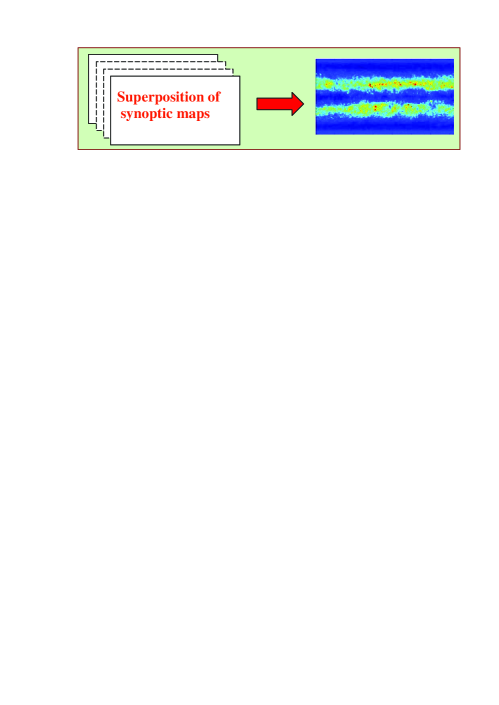
Figure 1.: Scheme of the method. Summing up synoptic maps of the photospheric magnetic field results in a synoptic map that represents the distribution of the photospheric magnetic field averaged over the entire period of $1976-2003$.summethod

To give an idea of the characteristics of the data we used and of the order of magnitude of the magnetic fluxes, we show the change of the magnetic flux for years $1976-2003$ in Figure totalflux, evaluated for each synoptic map and then averaged using running means over 20 rotations. The photospheric magnetic flux changes in phase with the solar activity. The maximum of the flux coincides with the second Gnevyshev maximum; the maximum fluxes occur in 1981.4, 1991.6, and 2002.2.

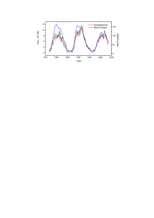
Figure 2.: Photospheric magnetic flux during Solar Cycles $21-23$ (thin black line). The red line represents smoothed moving averages over 20 Carrington Rotations. Wolf numbers are plotted with the blue line. The total magnetic flux approximately follows the evolution of the sunspot number.totalflux

The averaged latitudinal profile of the magnetic field (Figure totalprofile) shows two domains where the magnetic flux increases: at the latitudes of the sunspot zone and at the latitudes of the polar facular zone. The flux in the sunspot zone considerably exceeds the flux in the polar facular zone.

It should be mentioned that some very low (background) flux exists at each latitude (approximately $1.3\times 10^{21}$ G). The maximum in the sunspot zone exceeds the background flux by five times. One can note that the total flux averaged over three cycles for the southern hemisphere exceeds the flux in the northern hemisphere.

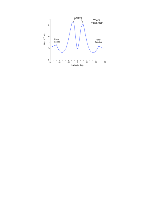
Figure 3.: Latitudinal profile of the magnetic field averaged over Solar Cycles $21-23$. The magnetic flux was normalized to the number of rotations included in the resulting map. Concentrations of the magnetic field are observed in the sunspot zone and at the latitudes characteristic of polar faculae.totalprofile

3 Results and Discussion

resdis

When studying the latitudinal distributions of magnetic fields of different magnitude, we discovered that there are four characteristic groups of fields. These are fields with strengths in ranges of $0-5$ G, $5-15$ G, $15-50$ G, and $B>50$ G. Magnetic fields in each of the groups have common latitudinal distribution features, while for different field groups these features change significantly. Each of the groups is closely related to a certain manifestation of the solar activity.

To study the latitudinal distribution of these groups we obtained separate summary magnetic field maps for each of the above field ranges. Before the summation, each synoptic map was transformed in such a way that only the pixels in the field strength range under consideration are taken into account. Namely, the value of $B$ for each pixel was replaced by 1 or 0 according to whether $B$ fell into the $B_{min}-B_{max}$ range or not. Thus, we obtained the summary map for the three solar cycles for the given range of magnetic field strength. This map shows the percentage of time when the fields of the given group at a given location were present on the solar surface.

We show the summary map for the group of the strongest magnetic fields over 50 G in Figure stronga. These fields occupy the sunspot zone and are obviously connected with the active regions on the Sun. On the right,we give the scale that shows the percentage of time when the fields from this group were observed at each location. The maximum of the scale is about $15\,\%$. Dark blue and blue correspond to rare appearance of the magnetic fields in the given strength range (less than $5\,\%$ of time), while yellow and red correspond to a frequent presence of the field strength range considered ($10-15\,\%$ of the observation time). By averaging the summary map over the longitude, we obtained the latitudinal profile of the magnetic flux (Figure strongb). The magnetic flux was normalized to the number of rotations included into the resulting map. The latitudinal profile for this group of field strengths shows that strong magnetic fields are only observed in the sunspot zones.

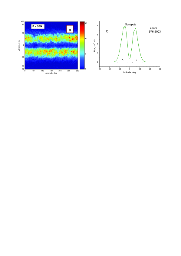
Figure 4.: Latitudinal distribution of strong magnetic fields ($B>50$ G). a) Summary magnetic field map for three solar cycles. To the right we show a color bar indicating the percentage of time for which the fields with strength $B>50$ G were observed (the maximum of the scale is $15\,\%$). b) The latitudinal profile for this group of fields shows that strong magnetic fields were only present in the sunspot zones (the latitudinal ranges are marked A and B).strong

In Figure medium the next group of magnitudes from 15 to 50 G is considered. The summary map shows that each hemisphere has two dominant regions corresponding to the sunspot zone and the polar facular zone. The sunspot zone occupies a wider strip of latitudes than in Figure stronga (yellow and red strips at latitudes below $40^{\circ}$) and exists up to $25\,\%$ of the time. The polar facular zone occupies a narrow strip (yellow and light blue strips at latitudes around $70^{\circ}$), but it is clearly visible. This zone is even more pronounced in the latitudinal profile (Figure mediumb), where the maxima of facular concentration appear around latitudes $+70^{\circ}$ and $-70^{\circ}$.

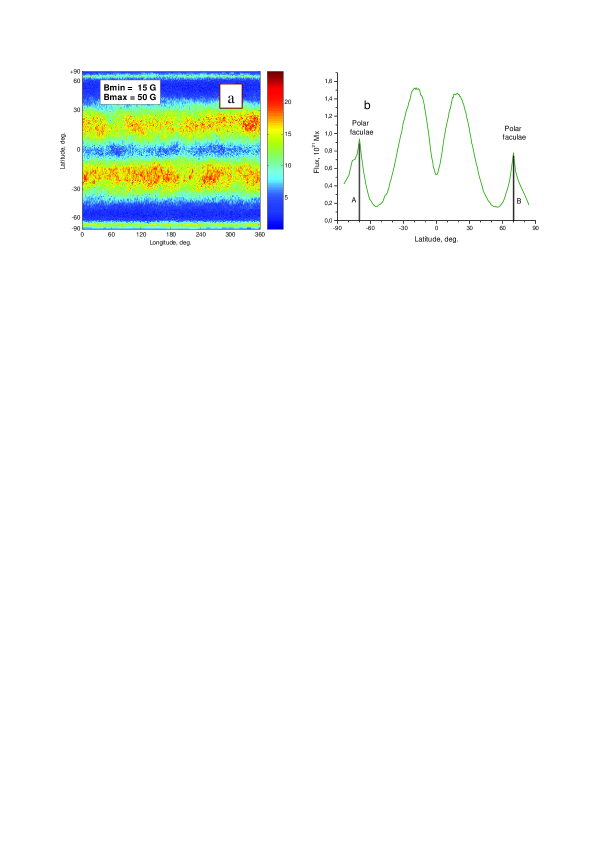
Figure 5.: Latitudinal distribution of magnetic fields in the $15-50$ G strength range. a) Summary map for three solar cycles. To the right we show a color bar indicating the percentage of time for which the fields with strength $B=15-50$ G were observed at a given location (the maximum of the scale is $25\,\%$). b) The latitudinal profile of the magnetic flux. Dominating regions: sunspot zone and zone of polar faculae (maxima of the polar faculae magnetic flux are marked A and B). medium

The group of fields with magnitudes from 5 to 15 G dominates in the summary map (Figure weaka) at the highest latitudes (yellow and red strips in the map) and exists up to $55\%$ of time. The lower limit of the color bar (dark blue color) in this map corresponds to $15\,\%$ of time. Thus the magnetic fields of this group appear over the whole solar disk for a significant part of the solar cycle. The latitudinal profile of the magnetic flux (Figure weakb) shows a sharp increase of the flux from latitudes around $60^{\circ}$ toward the poles. The strength and localization of these fields indicate their connection with the polar coronal holes.

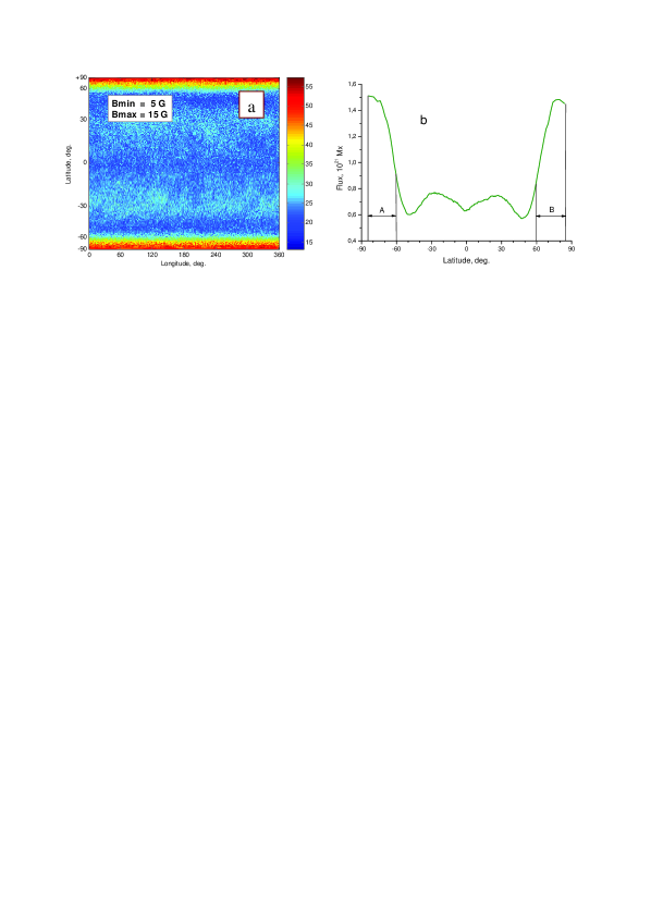
Figure 6.: Latitudinal distribution of magnetic fields in the $5-15$ G strength range. a) Summary map for three solar cycles. To the right we show a color bar indicating the percentage of time for which the fields with strength $B=5-15$ G were observed at a given location (the maximum of the scale is $55\,\%$). b) The latitudinal profile of the magnetic flux. The strength and localization of these fields indicate their connection with the polar coronal holes (the latitudinal ranges are marked A and B). weak

The weakest magnetic fields (lower than 5 G) occupy three regions in the summary map (Figure veryweaka): the equatorial region $\pm 5^{\circ}$, and latitudes from $60^{\circ}$ down to the sunspot zone in each of the hemispheres. As the color bar shows, weak fields are present more than $80\%$ of time. At other latitudes these fields appear at least for $35\,\%$ of time (dark blue strips near the solar poles). The latitudinal profile of the flux (Figure veryweakb) shows maxima at latitudes $0^{\circ}$ and $53^{\circ}$.

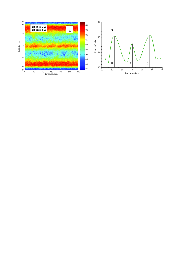
Figure 7.: Latitudinal distribution of magnetic fields in the $0-5$ G strength range. a) Summary map for three solar cycles. To the right we show a color bar indicating the percentage of time for which the fields with strength $B=0-5$ G were observed at a given location (the maximum of the scale is $80\,\%$). b) The latitudinal profile of the magnetic flux. The weakest fields are concentrated at the solar equator (the flux maximum is marked A) and within the latitude range $40^{\circ}-60^{\circ}$ (the flux maxima are marked B and C).veryweak

The latitudinal distribution in Figure strong shows that strong magnetic fields, $B>50$ G, are confined only within the sunspot zone. It is interesting to consider latitudinal distributions of magnetic fields with strengths below 50 G for 5 G strength bins. In Figure fivebin, we present the latitudinal profiles of the magnetic field for various strength ranges. The weakest (background) fields are concentrated near the equator and at latitudes around $50^{\circ}$. In these regions fields stronger than 10 G are almost absent.

The high-latitude measurements are less reliable because the magnetic field is radial in the photosphere and has only a small component in the line-of-sight direction where the instrument is sensitive. According to Harvey (1996), the instrumental noise level in the polar regions in NSO/KP maps is a function of latitude and is on the order of 2 G per map element. The influence of these measurement errors is diminished by the data treatment we used here. To obtain latitudinal profiles, synoptic maps were averaged in longitude and then averaged as a function of time for nearly three cycles. With this averaging the instrumental noise level near the poles is reduced significantly.

Latitudinal profiles for both $10-15$ G and $15-20$ G field groups change in antiphase with the weakest magnetic fields, $B=0-5$ G. Flux minima for the range $15-20$ G nearly coincide with the weak-field maxima. The fluxes of magnetic field in strength ranges of $B=0-5$ G and $B=15-20$ G, considered as functions of the latitude, display a strong anticorrelation (correlation coefficient $-0.94$).

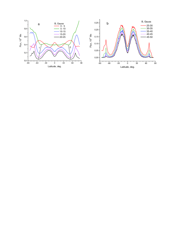
Figure 8.: Latitudinal profiles averaged over the period of $1976-2003$ for field groups from 0 to 25 G (panel a) and from 25 to 50 G (panel b). Straight lines 1 and 2 in panel a show the displacement of the profile minima.fivebin

In the polar regions the fields with strengths in the range $5-10$ G dominate; their concentration decreases sharply at latitudes $\pm 60^{\circ}$ when we move from the poles toward the equator. The magnetic flux in this range is nearly constant for all heliolatitudes except the highest ones, where it exceeds the flux values of all other field groups. For magnetic fields in the range $10-15$ G, the latitudinal profile has two maxima: in the sunspot zone and in the zone of polar faculae. This feature becomes more pronounced for higher magnetic strengths: $15-20$ G and $20-25$ G. It should be noted that the flux in the zone of polar faculae exceeds that of the sunspot zone for the weaker magnetic fields of $10-15$ G and $15-20$ G, whereas for the $20-25$ G group we observe a reversed relation.

In Figure fivebina the displacement of the minima toward higher latitudes can be seen for the magnetic fields with higher strengths. The minimum of the latitudinal distribution moves from $45^{\circ}$ for the $5-10$ G magnetic fields up to $55^{\circ}$ latitude for the $20-25$ G fields. In contrast, the distribution maxima in the sunspot zone move to the lower latitudes for greater strengths, although this displacement is rather small.

As the strength of the magnetic field increases, two concentration zones appear in the latitudinal distribution: the zone of polar faculae (maximum at $\sim 70^{\circ}$) and the sunspot region (maximum at $\sim 20^{\circ}$). This two-zone structure (sunspot region and polar facular zone) is seen especially clearly in Figure fivebinb for magnetic fields from $25-30$ G to $45-50$ G. The flux in the sunspot zone significantly exceeds that of the facular zone. Both fluxes decrease for greater magnetic field strengths. The last group ($45-50$ G) displays high flux in the sunspot zone along with a flux close to zero in the facular zone.

4 Conclusions

secconcl

The latitudinal distribution of photospheric magnetic fields was analyzed using synoptic maps of the NSO/KP ($1976-2003$). A close connection between the values of the magnetic field and their latitudinal localization was found, which persisted after averaging the magnetic fields over three solar cycles.

The following groups of field values were shown to dominate at different latitudes:

(a) from the equator to $5^{\circ}$, the weakest fields ($B=0-5$ G);

(b) within the latitude range $5^{\circ}-40^{\circ}$, the strong fields ($B>15$ G), sunspots and active regions;

(c) in the latitude range $40^{\circ}-60^{\circ}$, the weakest fields ($B=0-5$ G);

(d) in a narrow strip of latitudes around $70^{\circ}$, magnetic fields from 15 to 50 G, polar faculae;

(e) in high-latitude regions (latitudes higher than $60^{\circ}$), magnetic fields from 5 to 15 G, polar coronal holes.

The analysis of summary synoptic maps allowed us to distinguish four characteristic groups of field values: $B=0-5$ G, $B=5-15$ G, $B=15-50$ G, and $B>50$ G. Within each of these ranges, the magnetic fields have common latitudinal distribution features, while for different field groups these features are significantly different. For each of these field strength groups, their latitudinal localization persists when we average the magnetic fields over three solar cycles. Each of the considered groups of field values is closely related to a certain manifestation of the solar activity.

Acknowledgments

NSO/Kitt Peak data used here are produced cooperatively by NSF/NSO, NASA/GSFC, and NOAA/SEL. We thank the referee for many helpful comments.

References

- Akhtemov et al. (2015) Akhtemov, Z.S., Andreyeva, O.A., Rudenko, G.V., Stepanian, N.N., and Fainshtein, V.G.: 2015, Adv. Space Res. 55, 3, 968. ADS, DOI.
- Carrington (1858) Carrington, R.C.: 1858, Mon. Not. Roy. Astron. Soc. 19, 1, 1. ADS.
- Deng et al. (2013) Deng, L., Qu, Z., Dun, G., and Xu, C.: 2013, Pub. Astron. Soc. Japan 65, 1, 11. ADS, DOI.
- Durrant and Wilson (2003) Durrant, C.J., Wilson, P.R.: 2003, Solar Phys. 214, 23. ADS, DOI.
- Harvey (1996) Harvey, J.: 1996. http://www.noao.edu/noao/staff/jharvey/pole.ps.
- Hathaway (2015) Hathaway, D.H.: 2015, Living Rev. Solar Phys., 12, 4. http://www.livingreviews.org/lrsp-2015-4, DOI. ADS.
- Hoeksema (1991) Hoeksema, J.T.: 1991, J. Geomagn. Geoelectr. 43, Suppl., 59.
- Ivanov, Miletskii, and Nagovitsyn (2011) Ivanov, V.G., Miletskii, E.V., Nagovitsyn, Yu.A.: 2011, Astron. Reports 55, 10, 911. ADS, DOI.
- Li, Yun, and Gu (2001) Li, K.J., Yun, H.S., Gu, X.M.: 2011, Astron. J. 122, 4, 2115. ADS, DOI.
- Makarov and Makarova (1986) Makarov, V.I., Makarova, V.V.: 1986, J. Astrophys. Astr. 7, 113. ADS, DOI.
- Makarov and Makarova (1996) Makarov, V.I., Makarova, V.V.: 1996, Solar Phys. 163, 267. ADS, DOI.
- Miletsky, Ivanov, and Nagovitsyn (2015) Miletsky, E.V., Ivanov, V.G., Nagovitsyn, Yu.A.: 2015, Adv. Space Res. 55, 3, 780. ADS, DOI.
- Muñoz-Jaramillo et al. (2012) Muñoz-Jaramillo, A., Sheeley, N.R., Zhang, J., DeLuca, E.E.: 2012, Astrophys. J. 753, 2, 146. ADS, DOI.
- Murray (1992) Murray, N.: 1992, Solar Phys. 138, 419. ADS, DOI.
- Sheeley (1964) Sheeley, N.R., Jr.: 1964, Astrophys. J. 140, 731. ADS, DOI.
- Sheeley (1976) Sheeley, N.R., Jr.: 1976, J. Geophys. Res. 81, 3462. ADS, DOI.
- Sheeley (1991) Sheeley, N.R., Jr.: 1991, Astrophys. J. 374, 386. ADS, DOI.
- Sheeley (2008) Sheeley, N.R., Jr.: 2008, Astrophys. J. 680, 1553. ADS, DOI.
- Solanki, Wenzler, and Schmitt (2008) Solanki, S.K., Wenzler, T., Schmitt, D.: 2008, Astron. Astrophys. 483, 623. ADS, DOI.
- Ulrich (1993) Ulrich, R.K.: 1993, in Weiss, W.W., Baglin, A. (eds.), IAU Colloq. 137, Inside the Stars, Astron. Soc. Pac. CS 40, 25. ADS.
- Waldmeier (1935) Waldmeier, M.: 1935, Astron. Mitt. Zürich 14, 105. ADS.
- Waldmeier (1939) Waldmeier, M.: 1939, Astron. Mitt. Zürich 14, 470. ADS.
- Wang, Sheeley, and Nash (1991) Wang, Y.-M., Sheeley, N. R., Jr., Nash, A. G.: 1991, Astrophys. J. 383, 431. ADS, DOI.