Interpolating function and Stokes Phenomena

Abstract

When we have two expansions of physical quantity around two different points in parameter space, we can usually construct a family of functions, which interpolates the both expansions. In this paper we study analytic structures of such interpolating functions and discuss their physical implications. We propose that the analytic structures of the interpolating functions provide information on analytic property and Stokes phenomena of the physical quantity, which we approximate by the interpolating functions. We explicitly check our proposal for partition functions of zero-dimensional $\varphi^{4}$ theory and Sine-Gordon model. In the zero dimensional Sine-Gordon model, we compare our result with a recent result from resurgence analysis. We also comment on construction of interpolating function in Borel plane.

HRI/ST/1501

1 Introduction

In most non-exactly solvable problems, one tries to look for a small parameter or a large parameter so that we can set up a perturbative expansion. This perturbation series is typically an asymptotic series which is divergent and has zero radius of convergence. Often the perturbation series takes different forms depending on the argument of its expansion parameter. This behavior is known as the Stokes phenomenon [1]. For example, if we consider a physical quantity having an integral representation as in quantum field theory and string theory, then the integrand usually has multiple saddle points and its perturbative expansion with the parameter $g$ typically takes the form

$$\sum_{k}a_{0,k}g^{k}+e^{-S_{1}(g)}\sum_{k}a_{1,k}g^{k}+e^{-S_{2}(g)}\sum_{k}a_{2,k}g^{k}+\cdots,$$ (1.1)

where $S_{i}(g)$ is the “action” evaluated at each saddle point and each sum denotes the small-$g$ expansion around that saddle point. In standard situations, the weight $e^{-S_{i}(g)}$ is exponentially suppressed for real positive $g$ and vanishes as approaching $g\rightarrow+0$. In other words all the terms except the first one in (1.1) describe non-perturbative effects. However, if we change ${\rm arg}(g)$, then $S_{i}(g)$ might have negative real part. For this case, the weight $e^{-S_{i}(g)}$ is not exponentially suppressed but exponentially growing. This type of transition happens when we cross an anti-Stokes line given by ${\rm Re}(S_{i})=0$. On the other hand, the coefficients $a_{i,k}$ themselves might jump as we change ${\rm arg}(g)$. This happens when we cross a Stokes line defined by ${\rm Im}(S_{i})={\rm Im}(S_{j})$. Thus Stokes phenomena has deep connections to non-perturbative effects.

In most practical situations, we can access to only first few terms of a perturbation series around single saddle point for particular argument of expansion parameter. For this case, it is hard to find when Stokes phenomena occur and when contributions from other saddle points become important. In this paper we develop a tool to study Stokes phenomena in somewhat special situations.

Sometimes we can have two perturbative expansions of physical quantity around two different points in parameter space, for example, in theory with S-duality, field theory with gravity dual, lattice gauge theory with weak and strong coupling expansions, statistical system with high and low temperature expansions, and so on. One can then construct functions, which interpolate these two expansions. The most standard approach to this is (two-point) Padé approximant, which is a rational function having the two expansions up to some orders. Recently Sen has considered another type of interpolating function, which has the form of a Fractional Power of Polynomial (FPP) [2]. After a while, one of us has constructed a more general class of interpolating functions described by Fractional Powers of Rational function (FPR) [3], which includes the Padé approximant and FPP as special cases. It has turned out that these interpolating functions usually provide better approximations than each perturbative expansion in intermediate regime of the parameter, see [2, 3, 4, 5, 6, 7] for various applications. Although these are quite nice as first attempts, properties of interpolating functions themselves have not been extensively studied yet.

In this paper we propose new properties of the interpolating functions. We focus on analytic structure of the interpolating functions by treating them as complex functions and discuss their physical implications. The FPR is some power of a rational function and the rational function has poles and zeros. When the power is not integer, then the poles and zeros of the rational function give rise to branch cuts of the FPR. Here we propose that the branch cuts of the FPR encode information about the analytic property and Stokes phenomena of the physical quantity, which we try to approximate. More concretely we propose that each branch cut of the FPR has the following possible interpretations.

1. The branch cut is particular to the FPR and the artifact of the approximation. Namely, this type of branch cut is not useful to extract physical information.

2. The physical quantity, which we approximate by the FPR, has a branch cut near from the branch cut of the FPR. Namely, the branch cut of the FPR well approximates the “true” branch cut of the physical quantity.

3. Near the branch cut, one of perturbation series of the physical quantity changes its dominant part. This case is further separated into the following two possibilities.

   1. We have an anti-Stokes line of the perturbative expansion near the branch cut. Namely, although the perturbative series itself does not change its own form, contributions from other saddle points become dominant across the line. This possibility likely occurs for first branch cut measured from a specific axis where we construct interpolating functions.

   2. The perturbative series itself does change the form. Namely, we have a Stokes line near the branch cut, whose diagonal multiplier is different from 1. When we have a Stokes line across which sub-dominant parts of the perturbative series change, the FPR cannot detect this type of Stokes line.

We explicitly check our proposal in two examples: partition functions of the $\varphi^{4}$ theory and the Sine-Gordon model in zero dimensions. Similar features seem to appear also in other examples such as BPS Wilson loop in 4d $\mathcal{N}=4$ Super Yang-Mills theory, energy spectrum in 1d anharmonic oscillator etc [24]. We expect that our result is applicable in more practical problems, where we do not know exact solutions. One possible utility of such an analysis is that we can anticipate analytic property and Stokes phenomena of physical quantity by looking at analytic structures of interpolating functions.

This paper is organized as follows. In section 2 we introduce our interpolating functions described by the fractional power of rational functions (FPRs). In section 3 we study interpolating problem in the 0d $\varphi^{4}$ theory in great detail. We look at the analytic property of the interpolating function as a complex function and propose its physical interpretation. In section 4 we analyze the 0d Sine-Gordon model and check that our proposal is true also for this model. Section 5 is devoted to conclusion and discussions. In appendix A we compare our interpolating function with a recent result from resurgence analysis [20] in the 0d Sine-Gordon model. Our result implies that the FPR and resurgence play complementary role with each other. In appendix B we explain an attempt to construct interpolating function in Borel plane and test its utility in the 0d Sine-Gordon model. In appendix C we write down explicit forms for interpolating functions used in the main text.

2 Interpolating function

We introduce the interpolating functions in this section, which is essentially a review of [3]. Suppose that we wish to determine a function $F(g)$, which has the small-$g$ expansion $F_{s}^{(N_{s})}(g)$ and large-$g$ expansion $F_{l}^{(N_{l})}(g)$ taking the forms

$$F_{s}^{(N_{s})}(g)=g^{a}\sum_{k=0}^{N_{s}}s_{k}g^{k},\quad F_{l}^{(N_{l})}(g)=g^{b}\sum_{k=0}^{N_{l}}l_{k}g^{-k}.$$ (2.1)

We can then naively expect that these expansions approximate $F(g)$ as

$$F(g)=F_{s}^{(N_{s})}(g)+\mathcal{O}(g^{a+N_{s}-1})=F_{l}^{(N_{l})}(g)+\mathcal{O}(g^{b-N_{l}-1}).$$ (2.2)

Although this seems to be a somewhat limited case, this situation includes a large class of physical problems, e.g., theory with S-duality, field theory with gravity dual, lattice gauge theory with weak and strong coupling expansions, statistical system with high and low temperature expansions, and etc.

In terms of the two expansions, one can construct the following function [3]

$$F_{m,n}^{(\alpha)}(g)=s_{0}g^{a}\Biggl{[}\frac{1+\sum_{k=1}^{p}c_{k}g^{k}}{1+\sum_{k=1}^{q}d_{k}g^{k}}\Biggr{]}^{\alpha},$$ (2.3)

where

$$p=\frac{1}{2}\left(m+n+1-\frac{a-b}{\alpha}\right),\quad q=\frac{1}{2}\left(m+n+1+\frac{a-b}{\alpha}\right).$$ (2.4)

The coefficients $c_{k}$ and $d_{k}$ are determined such that series expansions of $F_{m,n}^{(\alpha)}(g)$ around $g=0$ and $g=\infty$ reproduce the small-$g$ and large-$g$ expansions (2.1) of $F(g)$ up to $\mathcal{O}(g^{a+m+1})$ and $\mathcal{O}(g^{b-n-1})$, respectively. Due to this property, the function $F_{m,n}^{(\alpha)}(g)$ interpolates the small-$g$ and large-$g$ expansions up to these orders. Since the interpolating function is usually described by the Fractional Power of Rational function, we call this type of the interpolating function “FPR”. Note that the rational function inside the square bracket in (2.3) is a ratio of polynomials, i.e.,

$$p,q\in\mathbb{Z}_{\geq 0},$$ (2.5)

which leads the following condition

$$\alpha=\left\{\begin{matrix}\frac{a-b}{2\ell+1}&{\rm for}&m+n:{\rm even}\cr\frac{a-b}{2\ell}&{\rm for}&m+n:{\rm odd}\end{matrix}\right.,\quad{\rm with}\ \ell\in\mathbb{Z}.$$ (2.6)

It is now easy to see that the FPR includes the Padé approximant and the Fractional Power of Polynomial (FPP) constructed in [2] as special cases. If we take $2\ell+1=a-b$ for $a-b\in\mathbb{Z}$ and $m+n$ to be even, then this becomes the Padé approximant while if we take $2\ell+1=m+n+1$ ($2\ell=m+n+1$) for even (odd) $m+n$ then we get the FPP. Therefore we below refer to also the Padé and FPP as FPR.

3 Partition function of zero-dimensional $\varphi^{4}$ theory

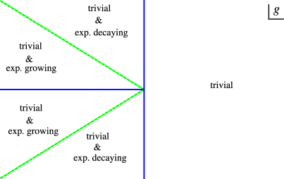
Figure 1: Summary of Stokes phenomena for the small-$g$ expansion in the partition function of the 0d $\varphi^{4}$ theory. The blue solid lines denote the Stokes lines while the green dashed lines denote the anti-Stokes lines.

In this section we study interpolation problem for the partition function of the 0d $\varphi^{4}$ theory. Although this example has been already studied well in [2, 3] for real non-negative coupling constant, here we consider general complex coupling. As mentioned above, we study analytic properties of interpolating functions and their physical implications. Let us consider the integral

$$F(g)=\frac{1}{\sqrt{g}}\int_{-\infty}^{\infty}dx\ e^{-\frac{x^{2}}{2g}-x^{4}},$$ (3.1)

which can be exactly performed as

$$F(g)=\left\{\ \begin{matrix}\frac{\pi e^{\frac{1}{32g^{2}}}}{4g}\left[I_{-\frac{1}{4}}\left(\frac{1}{32g^{2}}\right)-I_{\frac{1}{4}}\left(\frac{1}{32g^{2}}\right)\right]&{\rm for}\ {\rm Re}(g)>0\cr\cr\frac{\pi e^{\frac{1}{32g^{2}}}}{4\sqrt{-g^{2}}}\left[I_{-\frac{1}{4}}\left(\frac{1}{32g^{2}}\right)+I_{\frac{1}{4}}\left(\frac{1}{32g^{2}}\right)\right]&{\rm for}\ {\rm Re}(g)\leq 0\cr\end{matrix}\right.,$$ (3.2)

where $I(z)$ is the modified Bessel function of the first kind. The small-$g$ expansion of $F(g)$ depends on the argument of $g$, and its dependence is given by

$$F(g)=\left\{\begin{matrix}\sqrt{2\pi}-3\sqrt{2\pi}g^{2}+105\sqrt{\frac{\pi}{2}}g^{4}+\mathcal{O}(g^{6})&{\rm for}\ {\rm arg}(g)\in(-\frac{\pi}{2},\frac{\pi}{2})\cr\sqrt{\frac{\pi}{2}}\left(105g^{4}-6g^{2}+2+\mathcal{O}(g^{6})\right)-\sqrt{\pi}ie^{\frac{1}{16g^{2}}}\left(105g^{4}+6g^{2}+2+\mathcal{O}(g^{6})\right)&{\rm for}\ {\rm arg}(g)\in(\frac{\pi}{2},\pi)\cr\sqrt{\frac{\pi}{2}}\left(105g^{4}-6g^{2}+2+\mathcal{O}(g^{6})\right)+\sqrt{\pi}ie^{\frac{1}{16g^{2}}}\left(105g^{4}+6g^{2}+2+\mathcal{O}(g^{6})\right)&{\rm for}\ {\rm arg}(g)\in(-\pi,-\frac{\pi}{2})\cr\end{matrix}\right..$$ (3.3)

This dependence on ${\rm arg}(g)$ clearly reflects the fact that we have Stokes lines oriented along ${\rm arg}(g)=\pm\pi/2$ and $\pi$, across which the form of the small-$g$ expansion changes. Notice that across the ray $|{\rm arg}(g)|>3\pi/4$, the terms involving the exponential factor (in line 2 and 3 in eq. (3.3)) are dominant compared to those without the exponential factor. This indicates that we have the anti-Stokes lines oriented along ${\rm arg}(g)=\pm 3\pi/4$.

It is easy to understand this behavior from the standard saddle point analysis for $|g|\ll 1$. Saddle points $x_{\ast}$ of the integration are given by

$$x_{\ast}=0,x_{\pm},\quad{\rm with}\ x_{\pm}=\pm\frac{i}{2\sqrt{g}}.$$ (3.4)

Then, the “action” $S(x)=\frac{x^{2}}{2g}+x^{4}$ at the saddle points $x_{\ast}$ takes the values

$$S(x_{\ast}=0)=0,\quad S(x_{\ast}=x_{\pm})=-\frac{1}{16g^{2}}.$$ (3.5)

For $|{\rm arg}(g)|<\pi/2$, we can pick up only the trivial saddle point $x_{\ast}=0$ by deforming the original integral contour $(-\infty,\infty)$ to a steepest descent contour, while we can pick up all the saddle points otherwise. We have relative minus sign in the contributions from the non-trivial saddle points $x_{\ast}=x_{\pm}$ because directions of the steepest descent through $x_{\ast}=x_{\pm}$ are opposite between the cases for $\pi/2<{\rm arg}(g)<\pi$ and $-\pi<{\rm arg}(g)<-\pi/2$. Note that the real parts of the action at the non-trivial saddle points change their signs across ${\rm arg}(g)=\pm 3\pi/4$. This means that we have anti-Stokes lines of the small-$g$ expansion at ${\rm arg}(g)=\pm 3\pi/4$. This discussion is summarized in fig. 1. The large-$g$ expansion, on the other hand, is independent of ${\rm arg}(g)$:

$$F(g)=g^{-1/2}\left(\frac{1}{2}\Gamma(1/4)+\frac{1}{16}\Gamma(-1/4)g^{-1}+\frac{1}{64}\Gamma(1/4)g^{-2}+\mathcal{O}(g^{-3})\right).$$ (3.6)

3.1 Interpolation along positive real axis

Let us first take the coupling $g$ to be real and positive as usual. For this case, we have the following small-$g$ and large-$g$ expansions

$$F_{s}^{(N_{s})}(g)=\sum_{k=0}^{N_{s}}s_{k}g^{k},\quad s_{2k+1}=0,\quad s_{2k}=\frac{\sqrt{2}\Gamma(2k+1/2)}{k!}(-4)^{k},$$ (3.7)

$$F_{l}^{(N_{l})}(g)=g^{-1/2}\sum_{l=0}^{N_{l}}l_{k}g^{-k},\quad l_{k}=\frac{\Gamma\left(\frac{k}{2}+\frac{1}{4}\right)}{2k!}\left(-\frac{1}{2}\right)^{k},$$ (3.8)

which are compared with the exact result in fig. 2 [Left]. In terms of these expansions, we can construct FPR-type interpolating function $F_{m,n}^{(\alpha)}(g)$ (see app. C.1 for explicit forms). In fig. 2 [Right], we test validity of the FPRs by plotting

$$\frac{F_{m,n}^{(\alpha)}-F(g)}{F(g)},$$

against $g$ for some $(m,n,\alpha)$. We easily see that these interpolating functions provide good approximations to the original function $F(g)$. Especially $F_{6,6}^{(1/2)}(g)$ approximates the exact result $F(g)$ very well: the maximal value of the ratio $|(F_{6,6}^{(1/2)}(g)-F(g))/F(g)|$ is $\mathcal{O}(10^{-8})$. Thus we find that our interpolating scheme in this example works quite well at least along the positive real axis of $g$. Of course this result is not new and has been already seen in the previous studies [2, 3]. Here we ask another question. Suppose we perform naive analytic continuation of the interpolating function $F_{m,n}^{(\alpha)}(g)$ to the whole complex plane of $g$. Then, does the interpolating function $F_{6,6}^{(1/2)}(g)$, which is very precise along the positive real $g$, still gives a good approximation beyond the positive real axis?

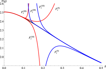
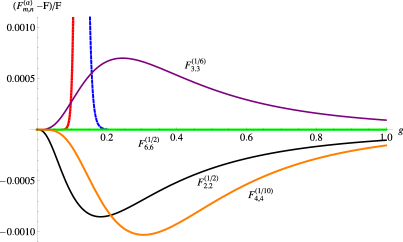
Figure 2: [Left] The partition function of the 0d $\varphi^{4}$ theory (black solid), its small-$g$ expansions $F_{s}^{(N_{s})}(g)$ (red dotted) and large-$g$ expansions $F_{l}^{(N_{l})}(g)$ (blue dashed) for ${\rm arg}(g)=0$. [Right] Comparison of the FPRs with some $(m,n,\alpha)$ on the non-negative real axis of $g$.

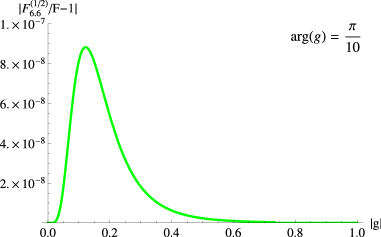
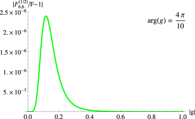
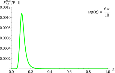
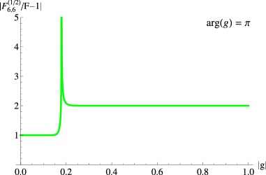
Figure 3: The quantity $|(F_{6,6}^{(1/2)}(g)-F(g))/F(g)|$ is plotted against $|g|$ for some ${\rm arg}(g)$.

In order to answer this question, we plot the quantity $|F_{6,6}^{(1/2)}(g)/F(g)-1|$ against $|g|$ for some ${\rm arg}(g)$ in fig. 3. First, we easily observe in fig. 3 [Left top] that the FPR gives very precise approximation for ${\rm arg}(g)=\pi/10$, whose relative error is $\mathcal{O}(10^{-7})$ at worst. Fig. 3 [Right top] shows that this is true also for ${\rm arg}(g)=4\pi/10$, albeit not as accurate as that for ${\rm arg}(g)=\pi/10$. We therefore conclude that the FPR can give good approximation of the exact function even beyond the real positive axis. However, as we further increase ${\rm arg}(g)$ to $\pi$, the approximation starts becoming worse. As seen in fig. 3 [Left bottom], the FPR still gives good approximation for ${\rm arg}(g)=6\pi/10$ but the relative error becomes $\mathcal{O}(0.1\%)$. Since we have the exponentially suppressed corrections in the weak coupling regime for $\pi/2<{\rm arg}(g)<3\pi/4$, which comes from the nontrivial saddle points, we recognize that the exponentially suppressed corrections are responsible for this error. For $3\pi/4<{\rm arg}(g)<5\pi/4$, the contributions from the nontrivial saddle points become exponentially growing. Since the FPR lacks this information, the FPR should show very large error for $3\pi/4<{\rm arg}(g)<5\pi/4$ in small-$|g|$ regime. Indeed we have $\mathcal{O}(100\%)$ error on the negative real axis as seen in fig. 3 [Right bottom]. In fig. 4, we summarize validity of approximation by the FPR. The shaded part shows the region where the FPR has more than $5\%$ relative error. We also draw the zeros and poles of the rational function $(F_{6,6}^{(\alpha)})^{2}$ associated with the FPR, which give branch cuts of the FPR.

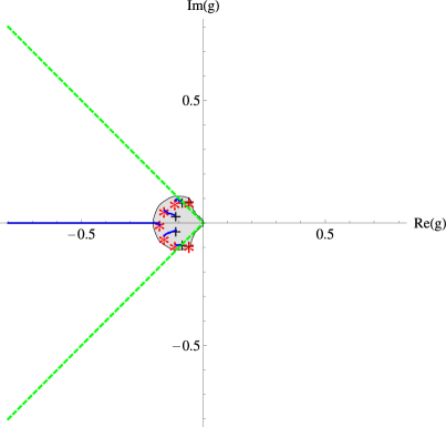
Figure 4: The region where the interpolating function $F_{6,6}^{(1/2)}(g)$ gives bad approximation. In the shaded region, the ratio $|F_{6,6}^{(1/2)}/F-1|$ is larger than $0.05$. We also plot “zeros” (the symbol “$+$”) and “poles” (the symbol “$\ast$”) of the rational function $(F_{6,6}^{(1/2)}(g))^{2}$ associated with the FPR. The blue solid lines denote the branch cuts of $F_{6,6}^{(1/2)}(g)$.

From this figure we observe some points:

• The shaded region looks like a fan, whose radial bounding lines are close to the anti-Stokes lines of the small-$g$ expansion. This is natural since the dominant part of the small-$g$ expansion changes across the anti-Stokes lines and the FPRs do not know this information in small-$|g|$ regime. The radius of the fan should be finite since the FPR gives the correct large-$g$ expansion by construction even across the anti-Stokes lines.

• The boundary of the (shaded) fan-like region is similar to the region surrounded by the origin, poles and zeros of the rational function $(F_{6,6}^{(1/2)}(g))^{2}$. Especially the anti-Stokes lines are close to the lines between the origin and the first poles measured from the positive real axis. This would be natural because when the exact function $F(g)$ does not have singularities around the poles of $(F_{6,6}^{(1/2)}(g))^{2}$, then the FPR differs from the exact function by a large amount in the neighborhood of its poles. Hence for this case, the FPR clearly gives bad approximation around the poles.

• There is a branch cut from the pole at the negative real axis to $g=-\infty$. Since the partition function $F(g)$ has the branch cut on $(0,-\infty)$, we interpret that the branch cut of the FPR approximates the “true” branch cut of the exact result.

• Although the small-$g$ expansion has the Stokes line at the imaginary axis, the FPR does not detect this Stokes line. This is because the dominant part of the small-$g$ expansion does not change across this Stokes line and only the sub-dominant part changes.

These results lead us to the conjecture about the general feature of FPR that each branch cut of the FPR has the following possible interpretations.

1. The branch cut is an artifact of the approximation by the FPR.

2. The physical quantity $F(g)$ has a branch cut near the branch cut of the FPR.

3. Near the branch cut, one of perturbation series of $F(g)$ changes its dominant part. This case implies the following two possibilities on Stokes phenomena.

   1. We have an anti-Stokes line of the perturbative expansion near the branch cut. This possibility occurs most likely for the first branch cut measured from the specific axis where the interpolating function is constructed.

   2. We have a Stokes line near the branch cut, whose diagonal multiplier is different from 1.

One of immediate questions here is if these features are particular for this problem or true also for other problems. We will explicitly check this in sec. 4 that this is true also for the partition functions of the 0d Sine-Gordon model. This seems to hold also in other examples such as BPS Wilson loop in 4d $\mathcal{N}=4$ Super Yang-Mills theory, energy spectrum in 1d anharmonic oscillator etc [24]. Another important question is if we can construct another interpolating function, which gives good approximation in the region, where the interpolating function along the positive real axis becomes bad. One natural way to do this is to construct interpolating functions along a specific axis with $|{\rm arg}(g)|>3\pi/4$, where dominant part of the small-$g$ expansion comes from the non-trivial saddle points, and then to extend these to the complex $g$. In next subsection, we will perform this by considering interpolating functions along the negative real axis.

Remarks

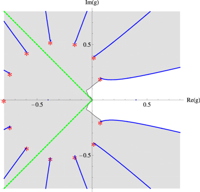
Figure 5: Similar plot as fig. 4 for the FPP $F_{6,6}^{(1/26)}(g)$.

One might ask if the FPRs $F_{m,n}^{(\alpha)}$ with the same $(m,n)$ but different $\alpha$ gave similar results. In this example we find that the results strongly depend on $\alpha$. For instance, let us look at fig. 5, which is similar to the plot in fig. 4 but for $F_{6,6}^{(1/26)}(g)$. Note that the FPR for this case becomes the FPP [2]. On the real positive axis, this interpolating function gives maximum error of about $0.6\%$. It is easy to see from fig. 5 that the analytic structure of $F_{6,6}^{(1/26)}(g)$ is very different from the one of $F_{6,6}^{(1/2)}(g)$. Especially, when we start from the real positive axis and go towards the anti-Stokes line at ${\rm arg}(g)=3\pi/4$, we encounter many branch cuts for this case. Another important difference is that the first branch cuts from the real positive axis are located at the pretty smaller angle ${\rm arg}(g)\simeq\pm 1.21$, which is quite far from the location of the anti-Stokes likes. This seems to be the reason why the FPP $F_{6,6}^{(1/26)}(g)$ gives the worse approximation than $F_{6,6}^{(1/2)}(g)$.

3.2 Interpolation along negative real axis

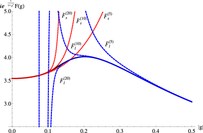
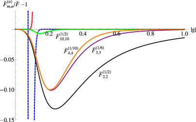
Figure 6: [Left] The function $\tilde{F}(g)=ie^{-\frac{1}{16g^{2}}}F(g)$ (black solid), its small-$g$ expansions $\tilde{F}_{s}^{(N_{s})}(g)$ (red dotted) and large-$g$ expansions $\tilde{F}_{l}^{(N_{l})}(g)$ (blue dashed) for ${\rm arg}(g)=\pi-\epsilon$. [Right] The quantity $(\tilde{F}_{m,n}^{(\alpha)}(t)/\tilde{F}(t)-1)=(F_{L+,m,n}^{(\alpha)}(-t)/F(-t)-1)$ is plotted to $t=|g|$.

In order to construct another interpolating function precise for $|{\rm arg}(g)|>3\pi/4$, let us consider interpolating function along the negative real axis of $g$ and then consider its naive analytic continuation to the whole complex plane. The function $F(g)$ has the following small-$g$ and large-$g$ expansions on $\epsilon$-neighborhood of the negative real axis:

$$F(-t+i\epsilon) = -\sqrt{\pi}ie^{\frac{1}{16t^{2}}}\left(2+6t^{2}+\mathcal{O}(t^{4})\right)+\sqrt{\frac{\pi}{2}}\left(2-6t^{2}+\mathcal{O}(t^{4})\right)+\mathcal{O}(\epsilon)\mbox{$$}$$

$$= -it^{-1/2}\left(\frac{1}{2}\Gamma(1/4)-\frac{1}{16}\Gamma(-1/4)t^{-1}+\frac{1}{64}\Gamma(1/4)t^{-2}+\mathcal{O}(t^{-3})\right)+\mathcal{O}(\epsilon),\mbox{$$}$$

$$F(-t-i\epsilon) = +\sqrt{\pi}ie^{\frac{1}{16t^{2}}}\left(2+6t^{2}+\mathcal{O}(t^{4})\right)+\sqrt{\frac{\pi}{2}}\left(2-6t^{2}+\mathcal{O}(t^{4})\right)+\mathcal{O}(\epsilon),\mbox{$$}$$

$$= +it^{-1/2}\left(\frac{1}{2}\Gamma(1/4)-\frac{1}{16}\Gamma(-1/4)t^{-1}+\frac{1}{64}\Gamma(1/4)t^{-2}+\mathcal{O}(t^{-3})\right)+\mathcal{O}(\epsilon),\mbox{$$}$$

with $t\in\mathbb{R}_{+}$. Namely, the dominant parts of the small-$g$ expansion and the large-$g$ expansion change their signs across the negative real axis. This reflects that the exact function $F(g)$ has the square root branch cut on the negative real axis. Instead of $F(g)$, let us consider interpolating functions of the quantity:

$$\tilde{F}(t)=\lim_{\epsilon\rightarrow+0}\left.ie^{-\frac{1}{16g^{2}}}F(g+i\epsilon)\right|_{g\rightarrow-t},\quad t\in\mathbb{R}_{+}.$$ (3.10)

The function $\tilde{F}(t)$ has the small-$t$ and large-$t$ expansions,

$$\tilde{F}(t) = 2\sqrt{\pi}+6\sqrt{\pi}t^{2}+105\sqrt{\pi}t^{4}+3465\sqrt{\pi}t^{6}+\frac{675675\sqrt{\pi}t^{8}}{4}+O\left(t^{10}\right)\mbox{$$}$$ (3.11)

$$= t^{-1/2}\left(\frac{\pi}{\sqrt{2}\Gamma\left(\frac{3}{4}\right)}+\frac{\pi t^{-1}}{8\sqrt{2}\Gamma\left(\frac{5}{4}\right)}-\frac{\pi t^{-2}}{32\sqrt{2}\Gamma\left(\frac{3}{4}\right)}-\frac{\pi t^{-3}}{256\sqrt{2}\Gamma\left(\frac{5}{4}\right)}+O\left(t^{-4}\right)\right),$$

where we have dropped the exponentially suppressed correction $\mathcal{O}(e^{-\frac{1}{16t^{2}}})$ coming from the trivial saddle point in the small-$t$ expansion. Denoting interpolating function of $\tilde{F}(t)$ as $\tilde{F}_{m,n}^{(\alpha)}(t)$, we can approximate the original function by using the function

$$F_{L\pm,m,n}^{(\alpha)}(g)=\mp ie^{+\frac{1}{16g^{2}}}\tilde{F}_{m,n}^{(\alpha)}(-g).$$ (3.12)

The interpolating function $F_{L\pm,m,n}^{(\alpha)}(g)$ reproduces the small-$g$ and large-$g$ expansions of $F(g)$ for $g\in\mathbb{R}_{-}\pm i\epsilon$ up to certain orders. Indeed $F_{L+,m,n}^{(\alpha)}(g)$ approximates $F(g)$ quite well along the negative real ($+i\epsilon$) axis as seen in fig. 6 [Right]. Especially $F_{L\pm,10,10}^{(\alpha)}(g)$ has about relative $0.8\%$ error at worst.

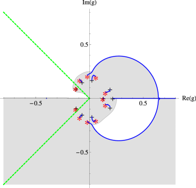
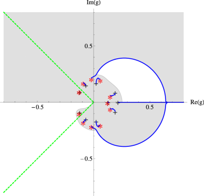
Figure 7: [Left] The region where the ratio $|F_{L+,10,10}^{(1/2)}/F-1|$ is larger than $0.05$. We also plot zeros ($+$) and poles ($\ast$) of the rational function $(\tilde{F}_{10,10}^{(1/2)})^{2}$. The blue solid lines denote the branch cuts of $F_{L+,10,10}^{(1/2)}$. [Right] Similar plot as the left for $F_{L-,10,10}^{(1/2)}$.

Let us consider general complex $g$ in the interpolating function $F_{L\pm,m,n}^{(\alpha)}(g)$ as in the last subsection. Then, unless we cross the anti-Stokes line or branch cuts, $F_{L\pm,m,n}^{(\alpha)}(g)$ gives the correct large-$g$ expansion and dominant part of small-$g$ expansion. If we cross the anti-Stokes line, then the small-$g$ expansion is dominated by the contribution from the trivial saddle point and $F_{L\pm,m,n}^{(\alpha)}(g)$ should fail to approximate $F(g)$ in small-$|g|$ regime. Also, if we cross the branch cut particular to the FPR, then the FPR will pick up an extra phase and also break the approximation. This extra phase could be trivial depending on the number of times, where we cross branch cuts.

The validity of the approximation by $F_{L\pm,10,10,}^{(-1/2)}(g)$ is summarized with its analytic property in fig. 7. One of important differences from the interpolation along the real positive axis is that the (semi-)circular branch cut of $F_{L\pm,10,10}^{(1/2)}(g)$ surrounds all the poles and zeros on the right plane. Therefore if we go across the circular branch cut on the right half plane, then $F_{L\pm,10,10}^{(1/2)}(g)$ undergoes a sign flip and hence it fails to approximate $F(g)$ across the circular branch cut. However, these FPRs also have a branch cut along the positive real axis and crossing this branch cut on the positive real axis leads to another flip in the sign. As a result $F_{L\pm,10,10}^{(1/2)}(g)$ recovers the correct sign and gives the good approximation to $F(g)$ again. That is why we see the disconnected unshaded regions in fig. 7.

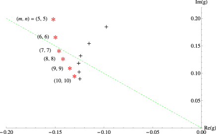
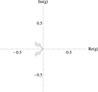
Figure 8: [Left] First poles and zeros of $(F_{m,n}^{(1/2)})^{2}$ from the negative real axis for various $(m,n)$. The symbol “+” denotes zeros and “*” denotes poles. [Right] The region where the patch $F^{\prime}(g)$ of the best FPRs gives more than relative $5\%$ error.

Another important difference is that the first branch cuts as measured from the negative real axis slightly deviate from the anti-Stokes lines. While the anti-stokes lines are oriented along ${\rm arg}(g)=\pm 3\pi/4\simeq\pm 2.356$, these first cuts are located at the angle ${\rm arg}(g)=\pm 2.504$. However, we expect that as increasing the values of $(m,n)$ in the FPR $F_{m,n}^{(1/2)}$, the first poles of $(F_{m,n}^{(1/2)})^{2}$ will approach to the first zeros from the negative real axis and the first cuts will finally vanish for sufficiently large $(m,n)$. Indeed we can easily observe in fig. 8 [Left] that the pair of first zeros and poles seem to converge to the same point as increasing $(m,n)$. Thus we conclude that the first pair of the branch cuts are the artifact of the approximation by the FPR with insufficiently large $(m,n)$. We call this type of singularities “fake singularities”. The above result would be natural because the FPR with larger $(m,n)$ tends to give better approximation in this problem and may improve the validity of the approximation near the anti-Stokes lines. In next section we will see that FPRs in the 0d Sine-Gordon model have similar features.

Finally let us find good approximation of $F(g)$ in region as wide as possible by patching the best interpolating functions along the positive and negative real axis. In fig, 8 [Right], we draw range of validity of approximation by

$$F^{\prime}(g)=\left\{\begin{matrix}F_{6,6}^{(1/2)}(g)&{\rm for}&|{\rm arg}(g)|<3\pi/4\cr F_{L+,10,10}^{(1/2)}(g)&{\rm for}&3\pi/4<{\rm arg}(g)<\pi\cr F_{L-,10,10}^{(1/2)}(g)&{\rm for}&-\pi<{\rm arg}(g)<-3\pi/4\cr\end{matrix}\right..$$ (3.13)

This indicates that the patching $F^{\prime}(g)$ has $5\%$ or better accuracy in the very wide region.

4 Partition function of zero-dimensional Sine-Gordon model

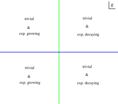
Figure 9: Summary of Stokes phenomena for the small-$g$ expansion in the partition function of the 0d Sine-Gordon model. The blue solid lines denote the Stokes lines while the green dashed lines denote the anti-Stokes lines.

Let us consider the partition function of the zero-dimensional Sine-Gordon model:

$$F(g)=\frac{1}{\sqrt{g}}\int_{-\pi/2}^{\pi/2}dx\ e^{-\frac{1}{2g}\sin^{2}{x}},$$ (4.1)

which was considered by Cherman-Koroteev-Unsal in the context of resurgence [20]. As in the last section, this integral can be evaluated exactly as

$$F(g)=\frac{\pi}{\sqrt{g}}e^{-\frac{1}{4g}}I_{0}\left(\frac{1}{4g}\right).$$ (4.2)

The function $F(g)$ has the following small-$g$ and large-$g$ expansions

$$F(g)=\left\{\begin{matrix}\sqrt{\frac{\pi}{32}}(8+4g+9g^{2}+\mathcal{O}(g^{3}))&{\rm for}\ {\rm arg}(g)=0\cr\sqrt{\frac{\pi}{32}}(8+4g+9g^{2}+\mathcal{O}(g^{3}))-i\sqrt{\frac{\pi}{32}}e^{-\frac{1}{2g}}(8-4g+9g^{2}+\mathcal{O}(g^{3}))&{\rm for}\ {\rm arg}(g)\in(0,\pi)\cr\sqrt{\frac{\pi}{32}}(8+4g+9g^{2}+\mathcal{O}(g^{3}))+i\sqrt{\frac{\pi}{32}}e^{-\frac{1}{2g}}(8-4g+9g^{2}+\mathcal{O}(g^{3}))&{\rm for}\ {\rm arg}(g)\in(-\pi,0)\cr\end{matrix}\right.,$$ (4.3)

while large-$g$ expansion is given by

$$F(g)=\pi g^{-1/2}\left(1-\frac{1}{4}g^{-1}+\frac{3}{64}g^{-2}-\frac{5}{768}g^{-3}+\mathcal{O}(g^{-4})\right).$$ (4.4)

Notice that the small-$g$ expansion has a Stokes line at arg$(g)=0,\ \pi$ and anti-Stokes lines at arg$(g)=\pm\pi/2$ as summarized in fig. 9. We can again understand this from the viewpoint of saddle points analysis. Saddle points of the integration are given by $x_{\ast}=0,\pm\pi/2$. At the saddle points, the action $S(x)=\frac{1}{2g}\sin^{2}{x}$ takes the values

$$S(x_{\ast}=0)=0,\quad S(x_{\ast}=\pm\pi/2)=\frac{1}{2g}.$$ (4.5)

We can pick up all the saddle points through steepest descent except for ${\rm arg}(g)=0$. We again have relative minus sign in the contributions from the non-trivial saddle points $x_{\ast}=\pm\pi/2$ because directions of the steepest descent through $x_{\ast}=\pm\pi/2$ are opposite between the cases for $0<{\rm arg}(g)<\pi$ and $-\pi<{\rm arg}(g)<0$. As in the 0d $\varphi^{4}$ theory, below we consider interpolating functions along the positive and negative real axis, and study their analytic properties as complex functions.

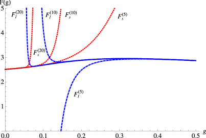
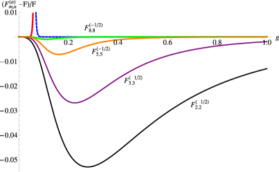
Figure 10: [Left] The partition function of the 0d Sine-Gordon model (black solid), its small-$g$ expansions $F_{s}^{(N_{s})}(g)$ (red dotted) and large-$g$ expansions $F_{l}^{(N_{l})}(g)$ (blue dashed) for ${\rm arg}(g)=0$. [Right] The function $(F_{m,n}^{(\alpha)}/F-1)$ is plotted to $g$ for some $(m,n,\alpha)$.

4.1 Interpolation along positive real axis

We start with interpolating functions along the non-negative real axis of $g$ and then analytically continue to complex coupling. For this case, we have the following small-$g$ and large-$g$ expansions

$$F_{s}^{(N_{s})}(g)=\sum_{k=0}^{N_{s}}s_{k}g^{k},\quad s_{k}=\sqrt{2\pi}\frac{2^{k}\Gamma^{2}(k+1/2)}{\Gamma(k+1)\Gamma^{2}(1/2)},\mbox{$$}$$

$$F_{l}^{(N_{l})}(g)=g^{-1/2}\sum_{l=0}^{N_{l}}l_{k}g^{-k},\quad l_{k}=\sqrt{\pi}\frac{\Gamma(k+1/2)}{\Gamma(k+1)},$$ (4.6)

which are compared with the exact result in fig. 10 [Left]. In terms of these expansions, we can construct interpolating function $F_{m,n}^{(\alpha)}(g)$ (see app. C.2 for explicit forms).

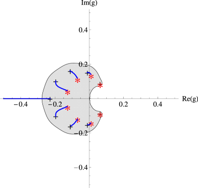
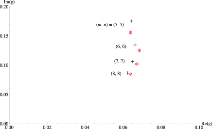
Figure 11: [Left] In the shaded region, the ratio $|F_{8,8}^{(-1/2)}/F-1|$ is larger than $0.05$. We also plot zeros ($+$) and poles ($\ast$) of $F_{8,8}^{(-1/2)}(g)$. The blue solid line denotes the branch cuts. [Right] First poles and zeros of $(F_{m,n}^{(-1/2)})^{2}$ from the positive real axis for various $(m,n)$.

In fig. 10 [Right], we compare some FPRs with the exact result for ${\rm arg}(g)=0$. As in the 0d $\varphi^{4}$ theory, we find that these interpolating functions well approximate the exact result for positive real $g$. For example, the best approximation $F_{8,8}^{(-1/2)}(g)$ among the FPRs has $\mathcal{O}(0.1\%)$ error at worst. Next let us consider complex $g$ in the best FPR $F_{8,8}^{(-1/2)}(g)$. We summarize the validity of the approximation with analytic structures of $F_{8,8}^{(-1/2)}(g)$ in fig. 11 [Left]. The shaded region again starts with the first branch cuts seen from the positive real axis, which are given by the first poles and zeros of the rational function $(F_{8,8}^{(-1/2)}(g))^{2}$. The first poles are located at ${\rm arg}(g)\simeq\pm 0.9348$, which is not near from the anti-Stokes lines at ${\rm arg}(g)=\pi/2\simeq\pm 1.571$. We again expect that the first branch cuts will vanish as increasing $(m,n)$ in $F_{m,n}^{(-1/2)}(g)$. Indeed fig. 11 [Right] implies that the first poles will collapse to the first zeros for large $(m,n)$ as in sec. 3.2. Hence we conclude that the branch cuts are the fake singularities and the FPR $F_{m,n}^{(-1/2)}(g)$ with sufficiently large $(m,n)$ would give good approximation in the right-half plane of $g$. In next subsection, we aim to construct interpolating functions approximating the exact result on the left-half plane by considering interpolating problem along the negative real axis.

4.2 Interpolation along negative real axis

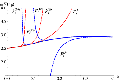
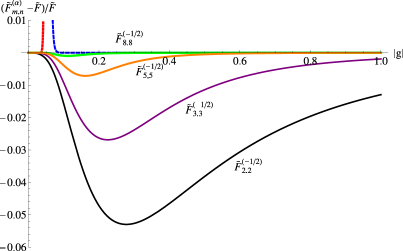
Figure 12: [Left] The function $\tilde{F}(g)=ie^{\frac{1}{2g}}F(g)$ (black solid), its small-$g$ expansions $\tilde{F}_{s}^{(N_{s})}(g)$ (red dotted) and large-$g$ expansions $\tilde{F}_{l}^{(N_{l})}(g)$ (blue dashed) for ${\rm arg}(g)=\pi-\epsilon$. [Right] The relative error $(\tilde{F}_{m,n}^{(\alpha)}/\tilde{F}-1)$ is plotted to $|g|$ for real negative $g$.

Let us consider interpolating problem along the negative real axis. The function $F(g)$ has the following expansions

$$F(-t+i\epsilon) = \sqrt{\frac{\pi}{32}}(8-4t+9t^{2}+\mathcal{O}(t^{3}))-i\sqrt{\frac{\pi}{32}}e^{\frac{1}{2t}}(8+4t-9t^{2}+\mathcal{O}(t^{3}))+\mathcal{O}(\epsilon)\mbox{$$}$$

$$= -it^{-1/2}\left(\pi+\frac{1}{4}\pi t^{-1}+\frac{3}{64}\pi t^{-2}+\frac{5}{768}\pi t^{-3}+\mathcal{O}(t^{-4})\right)+\mathcal{O}(\epsilon),\mbox{$$}$$

$$F(-t-i\epsilon) = \sqrt{\frac{\pi}{32}}(8-4t+9t^{2}+\mathcal{O}(t^{3}))+i\sqrt{\frac{\pi}{32}}e^{\frac{1}{2t}}(8+4t-9t^{2}+\mathcal{O}(t^{3}))+\mathcal{O}(\epsilon),\mbox{$$}$$ (4.7)

$$= +it^{-1/2}\left(\pi+\frac{1}{4}\pi t^{-1}+\frac{3}{64}\pi t^{-2}+\frac{5}{768}\pi t^{-3}+\mathcal{O}(t^{-4})\right)+\mathcal{O}(\epsilon),$$

with $t\in\mathbb{R}_{+}$. The dominant parts of the expansions change the signs across the negative real axis as in the $\varphi^{4}$ theory since $F(g)$ has the branch cut on the real negative axis. Hence it is more appropriate to consider the function

$$\tilde{F}(t)=\lim_{\epsilon\rightarrow+0}\left.ie^{\frac{1}{2g}}F(g+i\epsilon)\right|_{g\rightarrow-t},\quad t\in\mathbb{R}_{+}.$$ (4.8)

The function $\tilde{F}(t)$ has the expansions,

$$\tilde{F}(t) = \sqrt{2\pi}+\sqrt{\frac{\pi}{2}}t+\frac{9}{4}\sqrt{\frac{\pi}{2}}t^{2}+\frac{75}{8}\sqrt{\frac{\pi}{2}}t^{3}+\mathcal{O}(t^{4})\mbox{$$}$$ (4.9)

$$= t^{-1/2}\left(\pi-\frac{1}{4}\pi t^{-1}+\frac{3}{64}\pi t^{-2}-\frac{5}{768}\pi t^{-3}+\mathcal{O}(t^{-4})\right),$$

where we have dropped the exponentially suppressed correction $\mathcal{O}(e^{-\frac{1}{2t}})$ in the small-$g$ expansion (see fig. 12 [Left] for comparison of these expansions with the exact result of $\tilde{F}(t)$). Then we can construct the FPR $\tilde{F}_{m,n}^{(\alpha)}(t)$ to interpolate these expansions and approximate the original function $F(g)$ by

$$F_{L\pm,m,n}^{(\alpha)}(g)=\mp ie^{-\frac{1}{2g}}\tilde{F}_{m,n}^{(\alpha)}(-g).$$ (4.10)

The function $F_{L\pm,m,n}^{(\alpha)}(g)$ reproduces the small-$g$ and large-$g$ expansions of $F(g)$ for $g\in\mathbb{R}_{-}\pm i\epsilon$ up to certain orders.

In fig. 12 [Right] we check that the interpolating functions $\tilde{F}_{m,n}^{(\alpha)}(g)$ well approximate $\tilde{F}(g)$ on the negative real axis. We again summarize the validity of approximation by $F_{L\pm,9,9}^{(-1/2)}(g)$ and its analytic property in fig. 13. Starting with the negative real axis counterclockwise (clockwise), the approximation $F_{L+,9,9}^{(-1/2)}(g)(F_{L-,9,9}^{(-1/2)}(g))$ gets worse across the first branch cut as in last subsection, which is located around the line ${\rm arg}(g)\simeq(-)2.2578$ and deviates from the anti-Stokes lines. However, according to fig. 14 [Left], the first branch cuts seems to shrink as increasing $(m,n)$ in $(F_{L\pm m,n}^{(-1/2)}(g))^{2}$. Thus we expect that the branch cut is the fake singularity and the FPR $F_{L+,m,n}^{(-1/2)}(g)$ ($F_{L-,m,n}^{(-1/2)}(g)$) with sufficiently large $(m,n)$ well approximates $F(g)$ in the left-top-quarter (left-bottom-quarter) plane.

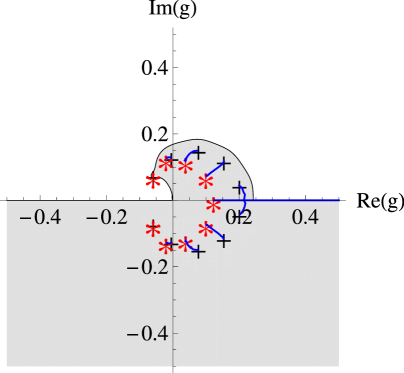
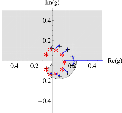
Figure 13: [Left] The region where the ratio $|F_{L+,9,9}^{(-1/2)}/F-1|$ is larger than $0.05$. We also plot zeros ($+$) and poles ($\ast$) of the rational function $(\tilde{F}_{10,10}^{(1/2)})^{2}$. The blue solid lines denote the branch cuts of $F_{L+,9,9}^{(-1/2)}$. [Right] Similar plot as the left for $F_{L-,9,9}^{(-1/2)}$.

Let us patch the best interpolating functions along the positive and negative real axis as in the $\varphi^{4}$ theory. In fig, 14 [Right], we draw range of validity of approximation by

$$F^{\prime}(g)=\left\{\begin{matrix}F_{8,8}^{(-1/2)}(g)&{\rm for}&|{\rm arg}(g)|<\pi/2\cr F_{L+,9,9}^{(-1/2)}(g)&{\rm for}&\pi/2<{\rm arg}(g)<\pi\cr F_{L-,9,9}^{(-1/2)}(g)&{\rm for}&-\pi<{\rm arg}(g)<-\pi/2\cr\end{matrix}\right..$$ (4.11)

This indicates that the patching $F^{\prime}(g)$ has $5\%$ or better accuracy in the fairly wide region.

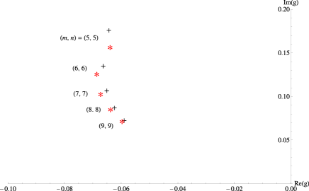
Figure 14: [Left] First poles and zeros of $(F_{L+,m,n}^{(-1/2)})^{2}$ from the positive real axis for various $(m,n)$. [Right] The region where the patch $F^{\prime}(g)$ of the best FPRs gives more than $5\%$ error.

5 Conclusion and Discussions

We have studied analytic structures of some interpolating functions and discussed their physical implications. We have proposed that the analytic structures of the interpolating functions provide information on analytic property and Stokes phenomena of the physical quantity, which we approximate by the interpolating functions. More concretely, we have mainly considered the roles of the first branch cuts measured from a specific axis where we construct the interpolating functions. If the first branch cuts are not “fake singularities”, then we expect that the cuts approximate those of the exact result or indicate locations of Stokes or anti-Stokes lines. When the cuts are fake singularities, we should consider next cuts in order to get physical implications. We have explicitly checked our proposal in the partition functions of the 0d $\varphi^{4}$ theory and the Sine-Gordon model. This seems to hold also in other examples such as BPS Wilson loop in 4d $\mathcal{N}=4$ Super Yang-Mills theory, energy spectrum in 1d anharmonic oscillator etc [24].

We expect that our result is applicable in more practical problems, where we do not know exact solutions. One possible application of our results is to use them to find Stokes behavior of the physical quantity by studying analytic structures of interpolating functions.

We have compared the result of the FPR with the recent result [20] of the resurgence in the 0d Sine-Gordon model. We have seen that the finite order approximation of the resurgence give better approximations than the FPR in the region where the FPR gives relatively imprecise approximation while the FPR is more precise in sufficiently strong coupling region. This implies that the FPR and resurgence play complementary roles. It will be interesting to compare them in more detail.

One of subtle points in our approach is concerned with the fake singularities. It is unclear how we should extend the definition of the fake singularities to more general problem. We have defined the fake singularity in our two examples as the branch cut shrinking for large $(m,n)$ with fixed $\alpha$. Since the relative errors seem to monotonically decrease as increasing $(m,n)$ in our examples, it would be reasonable to expect that the FPRs with sufficiently large $(m,n)$ have larger range of validity in the complex $g$-plane. However, in general problem, FPRs with larger $(m,n)$ do not necessarily give better approximations as seen in [3]. Natural extension of the definition would be to consider a family of FPRs $\{F_{m_{s},n_{s}}^{(\alpha_{s})}\}$ satisfying

$$\left|\frac{F_{m_{s},n_{s}}^{(\alpha_{s})}}{F(g)}-1\right|<\left|\frac{F_{m_{s+1},n_{s+1}}^{(\alpha_{s+1})}}{F(g)}-1\right|,$$ (5.1)

and define fake singularity as a cut, which shrinks as we increase $s$. It would be interesting to pursue this direction further.

In this paper we have focused on analytic properties of the best interpolating functions, which provide the best approximation among the given interpolating functions along a specific axis. However, when we do not know the exact results, it is nontrivial which interpolating functions give relatively better approximation as discussed in [3]. Although the work [3] has proposed a criterion to choose the best interpolating function in terms of two perturbative expansions, we need information on large order behavior of the expansions to use the criterion. It is nice if we use analytic properties of the interpolating functions to determine the relatively better interpolating functions without knowing exact results. In our examples, the exact results have the square-root type branch cuts. Interestingly the best interpolating functions are at $\alpha=\pm 1/2$ and hence also have the square-root type branch cuts. Thus the analytic properties of the interpolating functions would be helpful to improve such criterion.

We have seen that each FPR considered here has its own angular wedge of validity. By patching the best FPRs along the positive and negative real axis, we have obtained the approximation with larger range of validity than each FPR. It would be interesting if one can construct single interpolating function, which gives small-$g$ and large-$g$ expansions for all ${\rm arg}(g)$. One might think that this was conceptually similar to finding connection formula between different Stokes domains in exact JWKB method. However there are some important differences. One of such differences is that FPR often still gives good approximation even across Stokes line while approximation by FPR necessarily breaks down across the anti-Stokes line. For example, in the 0d $\varphi^{4}$ theory, the best FPR along the positive real axis gives precise approximation even across the Stokes line at ${\rm arg}(g)=\pi/2$ unless we approach to the anti-Stokes line at ${\rm arg}(g)=3\pi/4$. Thus the connection formula in JWKB does not seem to give useful hints. Let us see one of main difficulties to construct the single interpolating function valid for all ${\rm arg}(g)$ in the toy example:

$$F(g)=F_{0}(g)+e^{-\frac{1}{g}}F_{1}(g),\quad{\rm with}\ F_{0}(g)=\sum_{k=0}^{\infty}a_{0,k}g^{k},\ F_{1}(g)=\sum_{k=0}^{\infty}a_{1,k}g^{k},$$

where the summations $F_{0}(g)$ and $F_{1}(g)$ are convergent, and the exact result of $F(g)$ is given by their analytic continuations. Let us consider FPR to interpolate small-$g$ and large-$g$ expansions of $F(g)$. If we construct FPR along the positive real axis, then the FPR interpolates $F_{0}(g)$ and the large-$g$ expansion of $F(g)$. Some part of the information about the large-$g$ expansion is encoded in $F_{1}(g)$, but the FPR does not have this information in small-$g$ regime. This missing information gives exponentially suppressed error on the right plane of $g$ and exponentially growing error on the left plane for small $|g|$. Similarly if we construct FPR along the negative real axis, then that FPR does not have the information that a part of the large-$g$ expansion comes from $F_{0}(g)$. Of course we can find much better approximation in this example by separately constructing FPRs to interpolate $F_{0,1}(g)$ and large-$g$ expansion of analytic continuation of $F_{0,1}(g)$. However this information is almost equivalent to have the exact result and there is no motivation to perform this procedure.

Acknowledgments

We would like to thank Ashoke Sen for discussions and useful suggestions. DPJ would like to thank IMSc, Chennai and CHEP, Bengaluru for hospitality during the course of this work. This work was supported in parts by the DAE project 12-R& D-HRI-5.02.-0303.

Appendix A Comparison with resurgence result

As mentioned in the main text, the authors in [20] have performed resurgence analysis in the 0d Sine-Gordon model. It is interesting to compare their result with our interpolating functions. Their result is

$$F(g)=\left\{\begin{matrix}\mathcal{S}_{{\rm arg}(g)}\Phi_{0}(g)-ie^{-\frac{1}{2g}}\mathcal{S}_{{\rm arg}(g)}\Phi_{1}(g)&{\rm for}\ {\rm arg}(g)\in(0,\pi)\cr\mathcal{S}_{{\rm arg}(g)}\Phi_{0}(g)+ie^{-\frac{1}{2g}}\mathcal{S}_{{\rm arg}(g)}\Phi_{1}(g)&{\rm for}\ {\rm arg}(g)\in(-\pi,0)\cr\end{matrix}\right.,$$ (A.1)

where

$$\mathcal{S}_{\theta}\Phi_{0,1}(g)=\frac{1}{g}\int_{0}^{+\infty e^{i\theta}}dt\ e^{-\frac{t}{g}}\tilde{\mathcal{B}}\Phi_{0,1}(t).$$ (A.2)

The function $\tilde{\mathcal{B}}\Phi_{0}(t)$ ($\tilde{\mathcal{B}}\Phi_{1}(t)$) denotes analytic continuation of Borel transformation of the small-$g$ expansion coming from the saddle point $x_{\ast}=0$ ($x_{\ast}=\pm\pi/2$), which is explicitly given by

$$\tilde{\mathcal{B}}\Phi_{0}(t)=\sqrt{2\pi}\ _{2}F_{1}\left(\frac{1}{2},\frac{1}{2};1;2t\right),\quad\tilde{\mathcal{B}}\Phi_{1}(t)=\sqrt{2\pi}\ _{2}F_{1}\left(\frac{1}{2},\frac{1}{2};1;-2t\right).$$ (A.3)

Although we know all the coefficients of the small-$t$ expansions, let us consider finite order approximation of the resurgence result as in [20] and compare this with the FPRs. Namely, instead of using $\tilde{\mathcal{B}}\Phi_{0,1}(t)$, we terminate its small-$t$ expansion up to $\mathcal{O}(t^{2N+1})$ and use its one-point Padé approximant:

$$P^{(2N+1)}(t)=\frac{\sum_{k=0}^{N}c_{k}t^{k}}{1+\sum_{k=1}^{N}d_{k}t^{k}},$$ (A.4)

in the integration (A.2), which reproduces the small-$t$ expansion up to $\mathcal{O}(t^{2N+1})$. This procedure is often called (one-point) Borel-Padé approximation.

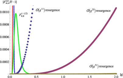
Figure 15: [Left] $|F_{8,8}^{(-1/2)}/F-1|$ for ${\rm arg}(g)=\frac{\pi}{100}$ [Right] The same plot as the left in a different scale.

In fig. 15, we compare the result of the resurgence with the FPR $F_{8,8}^{(-1/2)}$ for ${\rm arg}(g)=\frac{\pi}{100}$. By “$\mathcal{O}(g^{M})$ resurgence”, we mean the result obtained by the replacement $\tilde{\mathcal{B}}\Phi_{0,1}(t)\rightarrow P^{(M)}(t)$ in (A.2) and (A.1). We first find that the resurgence result gives very precise approximation in weak coupling regime. Furthermore all the results of the resurgence give better approximations in the region where the FPR gives relatively imprecise approximation. As we go to the large-$|g|$ regime, the approximation by the resurgence becomes monotonically worse but the $\mathcal{O}(g^{51})$ resurgence still gives reasonable approximation at $|g|=2$. However, if we further go to very large-$|g|$ regime, the approximation will breakdown. For example, the $\mathcal{O}(g^{51})$ resurgence has about $15\%$ error at $|g|=100$ and $140\%$ error at $|g|=1000$. Hence in sufficiently strong coupling regime, the FPR always gives the better approximation than the finite order approximation of the resurgence. This result implies that the FPR and resurgence play complementary roles in describing the exact function at least in this example. It will be interesting to compare them in more detail and other examples.

Appendix B Comments on interpolation in Borel plane

When small-$g$ (large-$g$) expansion of the function $F(g)$ is convergent, we expect that $F(g)$ is very precisely approximated by the FPRs $F_{m,n}^{(\alpha)}$ with large $m(n)$. How about the case where small-$g$ expansion is asymptotic but Borel summable? For this case, Borel transformation of the small-$g$ expansion is convergent. If we construct FPR-type interpolating function in the Borel plane, then one might expect that the “Borel-FPR” approximates the exact result of $F(g)$ very well. However, in this appendix, we discuss that the Borel-FPR gives slightly worse approximation than the usual FPR at least for the partition function of the 0d Sine-Gordon model. We have not understood any clear reasons behind this observation.

B.1 Method

Let us construct interpolating function for $F(g)$ in Borel plane. For this purpose, it is convenient to introduce following quantities:

$$\tilde{F}_{s}^{(N_{s})}(g)=g^{M}F_{s}^{(N_{s})}(g)=g^{\tilde{a}}\sum_{k=0}^{N_{s}}s_{k}g^{k},\quad\tilde{F}_{l}^{(N_{l})}(g)=g^{M}F_{l}^{(N_{l})}(g)=g^{\tilde{b}}\sum_{k=0}^{N_{l}}l_{k}g^{-k},$$ (B.1)

where

$$\tilde{a}=M+a,\quad\tilde{b}=M+b.$$ (B.2)

The parameter $M$ is a real number satisfying

$$\tilde{a}\geq 1,\quad\tilde{b}\geq N_{s}+1.$$ (B.3)

The Borel transformation of the small-$g$ expansion is

$$\mathcal{B}\tilde{F}_{s}^{(N_{s})}(t)=\sum_{k=0}^{N_{s}}\frac{s_{k}}{\Gamma(\tilde{a}+k)}t^{\tilde{a}+k-1}.$$ (B.4)

We also define action of $\mathcal{B}$ to the large-$g$ expansion as

$$\mathcal{B}\tilde{F}_{l}^{(N_{l})}(t)=\sum_{k=0}^{N_{l}}\frac{l_{k}}{\Gamma(\tilde{b}-k)}t^{\tilde{b}-k-1}.$$ (B.5)

Then we can construct the FPR-type interpolating function $\mathcal{B}F_{m,n}^{(\alpha)}(t)$ in Borel plane, which interpolate $\mathcal{B}\tilde{F}_{s}^{(N_{s})}(t)$ and $\mathcal{B}\tilde{F}_{l}^{(N_{l})}(t)$ up to $\mathcal{O}(t^{\tilde{a}+N_{s}})$ and $\mathcal{O}(t^{\tilde{b}-N_{l}-2})$, respectively:

$$\mathcal{B}F_{m,n}^{(\alpha)}(t)-\mathcal{B}\tilde{F}_{s}^{(N_{s})}(t)=\mathcal{O}(t^{\tilde{a}+N_{s}}),\quad\mathcal{B}F_{m,n}^{(\alpha)}(t)-\mathcal{B}\tilde{F}_{l}^{(N_{l})}(t)=\mathcal{O}(t^{\tilde{b}-N_{l}-2}).$$ (B.6)

This implies that the original function $F(g)$ is approximated by

$$F_{m,n}^{B(\alpha)}=g^{-M}\int_{0}^{\infty}dt\ e^{-\frac{t}{g}}\mathcal{B}F_{m,n}^{(\alpha)}(t),$$ (B.7)

which we call “Borel FPR”. Indeed one can show that the function $F_{m,n}^{B(\alpha)}$ gives $F_{s}^{(N_{s})}(g)$ in small-$g$ regime and $F_{l}^{(N_{l})}(g)$ in large-$g$ regime up to some orders. One of subtle points in this approach is that different values of $M$ give different $F_{m,n}^{B(\alpha)}$ even if we consider the same $(m,n,\alpha)$. In this paper, we will not study $M$-dependence and fix as $M=10$.

B.2 Comparison with usual interpolating function in 0d Sine-Gordon model

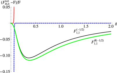
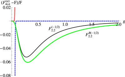
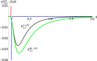
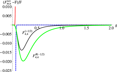
Figure 16: Comparison of the Borel FPR $F_{m,n}^{B(\alpha)}$ and usual FPR $F_{m,n}^{(\alpha)}$ for $(m,n)=(1,1),(2,2),(3,3),(4,4)$ with $(\alpha,M)=(-1/2,10)$.

Let us compare the Borel FPR with the usual FPR in the 0d Sine-Gordon model for ${\rm arg}(g)=0$. In fig. 16 we plot

$$\frac{F_{s}^{(20)}-F}{F},\quad\frac{F_{l}^{(20)}-F}{F},\quad\frac{F_{m,n}^{(-1/2)}-F}{F},\quad\frac{F_{m,n}^{B(-1/2)}-F}{F},$$

against $g$ for some values of $(m,n)$. We find that the Borel FPRs give slightly worse approximations than the usual FPRs with the same $(m,n,\alpha)$ at least for these four cases. This differs from our naive expectation and we have not found any clear reasons for that. We will not address this issue further, but it would be interesting to find some good interpretation or modification of our construction to get better approximation than the usual FPR.

Appendix C Explicit forms of interpolating functions

In this appendix, we write down explicit forms for interpolating functions used in the main text.

C.1 Partition function of 0d $\varphi^{4}$ theory

C.1.1 Interpolation along positive real axis of $g$

$$\scriptscriptstyle F_{0,0}^{(1/2)}(g)=\sqrt{2\pi}\left(\frac{8\pi g}{\Gamma\left(1/4\right)^{2}}+1\right)^{-1/2},\quad F_{1,1}^{(1/2)}(g)=\sqrt{2\pi\Gamma\left(1/4\right)}\left(\frac{8\pi g\Gamma\left(1/4\right)+\Gamma\left(1/4\right)^{3}+2\pi\Gamma\left(-1/4\right)}{64\pi^{2}g^{2}+8\pi g\Gamma\left(1/4\right)^{2}+\Gamma\left(1/4\right)^{4}+2\pi\Gamma\left(-1/4\right)\Gamma\left(1/4\right)}\right)^{1/2},\mbox{$$}$$

$$\scriptscriptstyle F_{1,1}^{(1/6)}(g)=2.50663\left(\frac{1}{6.98929g^{3}+7.08691g^{2}+1}\right)^{1/6},\quad F_{2,2}^{(1/2)}(g)=2.50663\sqrt{\frac{37.9117g^{2}+10.1532g+1}{72.4854g^{3}+43.9117g^{2}+10.1532g+1}},\mbox{$$}$$

$$\scriptscriptstyle F_{2,2}^{(1/10)}(g)=2.50663\left(25.5499g^{5}+43.1779g^{4}+32.1482g^{3}+30g^{2}+1\right)^{-1/10},\mbox{$$}$$

$$\scriptscriptstyle F_{3,3}^{(1/2)}(g)=2.50663\sqrt{\frac{324.019g^{3}+110.261g^{2}+16.0304g+1}{619.509g^{4}+420.201g^{3}+116.261g^{2}+16.0304g+1}},\mbox{$$}$$

$$\scriptscriptstyle F_{3,3}^{(1/6)}(g)=2.50663\left(\frac{28.2525g^{2}+8.0997g+1}{197.465g^{5}+256.834g^{4}+145.795g^{3}+46.2525g^{2}+8.0997g+1}\right)^{1/6},$$ (C.1)

$$\scriptscriptstyle F_{3,3}^{(1/14)}(g)=2.50663\left(93.3994g^{7}+220.976g^{6}+239.216g^{5}+155.758g^{4}+42g^{2}+1\right)^{-1/14},\mbox{$$}$$

$$\scriptscriptstyle F_{4,4}^{(1/2)}(g)=2.50663\sqrt{\frac{3224.56g^{4}+1303.49g^{3}+238.239g^{2}+22.8745g+1}{6165.22g^{5}+4576.g^{4}+1440.74g^{3}+244.239g^{2}+22.8745g+1}},\mbox{$$}$$

$$\scriptscriptstyle F_{4,4}^{(1/10)}(g)=2.50663\left[\frac{14.4369g^{2}+5.07251g+1}{368.86g^{7}+752.954g^{6}+708.689g^{5}+403.106g^{4}+152.175g^{3}+44.4369g^{2}+5.07251g+1}\right]^{1/10},\mbox{$$}$$

$$\scriptscriptstyle F_{4,4}^{(1/18)}(g)=2.50663\left(341.428g^{9}+1038.59g^{8}+1475.35g^{7}+1294.34g^{6}+780.788g^{5}+594g^{4}+54g^{2}+1\right)^{-1/18},\mbox{$$}$$

$$\scriptscriptstyle F_{5,5}^{(1/2)}(g)=1.8128\sqrt{\frac{(g+0.124648)(g^{2}+0.133925g+0.01439)(g^{2}+0.203814g+0.0156882)}{(g^{2}+0.144222g+0.0144064)(g^{2}+0.280251g+0.0278064)(g^{2}+0.375905g+0.0367401)}},\mbox{$$}$$

$$\scriptscriptstyle F_{6,6}^{(1/2)}(g)=1.8128\sqrt{\frac{(g^{2}+0.118257g+0.0116795)(g^{2}+0.172869g+0.0148819)(g^{2}+0.225907g+0.0137177)}{(g+0.179694)(g^{2}+0.118058g+0.011219)(g^{2}+0.234356g+0.0211961)(g^{2}+0.322914g+0.0291839)}},\mbox{$$}$$

$$\scriptscriptstyle F_{6,6}^{(1/26)}(g)=2.50663\bigl{(}4562.58g^{13}+20047.3g^{12}+42029.4g^{11}+55850.9g^{10}+52692.4g^{9}+37452.1g^{8}+20758.6g^{7}+9156.7g^{6}\mbox{$$}$$

$$\scriptscriptstyle\ \ \ \ \ \ \ \ \ \ \ +3248.63g^{5}+929.314g^{4}+213.078g^{3}+38.4914g^{2}+5.28292g+1\bigr{)}^{-\frac{1}{26}}.$$ (C.2)

C.1.2 Interpolation along negative real axis of $g$

$$\scriptscriptstyle\tilde{F}_{0,0}^{(1/2)}(t)=2\pi\sqrt{\frac{1}{8t\Gamma\left(\frac{3}{4}\right)^{2}+\pi}},\quad\tilde{F}_{1,1}^{(1/2)}(t)=2\pi\left(\frac{\Gamma\left(\frac{5}{4}\right)\left(8t\Gamma\left(\frac{3}{4}\right)^{2}+\pi\right)+2\Gamma\left(\frac{3}{4}\right)^{3}}{\Gamma\left(\frac{5}{4}\right)\left(64t^{2}\Gamma\left(\frac{3}{4}\right)^{4}+8\pi t\Gamma\left(\frac{3}{4}\right)^{2}+\pi^{2}\right)+2\pi\Gamma\left(\frac{3}{4}\right)^{3}}\right)^{1/2},\mbox{$$}$$

$$\scriptscriptstyle\tilde{F}_{2,2}^{(1/2)}(t)=6.28319\sqrt{\frac{0.0832t^{2}+0.0357t+0.00906}{t^{3}+0.0907t^{2}+0.1121t+0.0285}},\quad\tilde{F}_{3,3}^{(1/2)}(t)=1.81\sqrt{\frac{(t+0.398)\left(t^{2}+0.0631t+0.0634\right)}{\left(t^{2}-0.240t+0.105\right)\left(t^{2}+0.363t+0.0626\right)}},\mbox{$$}$$

$$\scriptscriptstyle\tilde{F}_{4,4}^{(1/2)}(t)=1.81\sqrt{\frac{t^{4}+0.40t^{3}+0.069t^{2}+0.015t+0.0044}{t^{5}+0.06t^{4}+0.081t^{3}+0.011t^{2}+0.0040t+0.00116}},\mbox{$$}$$

$$\scriptscriptstyle\tilde{F}_{5,5}^{(1/2)}(t)=1.81\sqrt{\frac{(t+0.30)\left(t^{2}-0.19t+0.044\right)\left(t^{2}+0.31t+0.050\right)}{\left(t^{2}-0.30t+0.063\right)\left(t^{2}+0.050t+0.076\right)\left(t^{2}+0.34t+0.037\right)}},\mbox{$$}$$

$$\scriptscriptstyle\tilde{F}_{6,6}^{(1/2)}(t)=1.8\sqrt{\frac{(t^{2}-0.23t+0.037)(t^{2}+0.10t+0.036)(t^{2}+0.51t+0.07)}{(t+0.18)(t^{2}-0.30t+0.050)(t^{2}-0.042t+0.07)(t^{2}+0.20t+0.042)}},\mbox{$$}$$

$$\scriptscriptstyle\tilde{F}_{7,7}^{(1/2)}(t)=2.\sqrt{\frac{(t+0.3)\left(t^{2}+0.003t+0.04\right)\left(t^{2}+0.4t+0.05\right)}{\left(t^{2}-0.1t+0.06\right)\left(t^{2}+0.1t+0.05\right)\left(t^{2}+0.4t+0.03\right)}},\mbox{$$}$$

$$\scriptscriptstyle\tilde{F}_{8,8}^{(1/2)}(t)=1.8\sqrt{\frac{\left(t^{2}-0.3t+0.03\right)\left(t^{2}-0.04t+0.03\right)\left(t^{2}+0.2t+0.02\right)\left(t^{2}+0.5t+0.06\right)}{(t+0.16)\left(t^{2}-0.3t+0.04\right)\left(t^{2}-0.14t+0.05\right)\left(t^{2}+0.09t+0.05\right)\left(t^{2}+0.2t+0.02\right)}},\mbox{$$}$$

$$\scriptscriptstyle\tilde{F}_{9,9}^{(1/2)}(t)=1.8\sqrt{\frac{(t+0.25)\left(t^{2}-0.25t+0.026\right)\left(t^{2}-0.1t+0.028\right)\left(t^{2}+0.09t+0.026\right)\left(t^{2}+0.4t+0.05\right)}{\left(t^{2}-0.27t+0.031\right)\left(t^{2}-0.16t+0.04\right)\left(t^{2}+0.019t+0.05\right)\left(t^{2}+0.13t+0.034\right)\left(t^{2}+0.35t+0.033\right)}},$$ (C.3)

C.2 Partition function of 0d Sine-Gordon model

C.2.1 Interpolation along positive real axis of $g$

$$\scriptscriptstyle F_{1,1}^{(-1/2)}(g)=\sqrt{2}\pi\left(\frac{2(2+\pi)g^{2}+3\pi g+(\pi-1)\pi}{(2+\pi)g+\pi-1}\right)^{-1/2},\quad F_{2,2}^{(-1/2)}(g)=\sqrt{2}\pi\left(\frac{32(8+5\pi+5\pi^{2})g^{3}+18\pi(9+8\pi)g^{2}+3\pi(37\pi-28)g+2\pi(10-35\pi+16\pi^{2})}{16\left(8+5\pi+5\pi^{2}\right)g^{2}+\left(-64+41\pi+32\pi^{2}\right)g+32\pi^{2}-70\pi+20}\right)^{-1/2},\mbox{$$}$$

$$\scriptscriptstyle F_{3,3}^{(-1/2)}(g)=3.14159\left(\frac{(g^{2}-0.0395594g+0.111122)(g^{2}+0.828493g+0.228908)}{(g+0.26163)(g^{2}+0.0273041g+0.0618949)}\right)^{-1/2},\mbox{$$}$$

$$\scriptscriptstyle F_{4,4}^{(-1/2)}(g)=3.14159\left(\frac{(g+0.403343)(g^{2}-0.10802g+0.0594072)(g^{2}+0.474071g+0.13076)}{\left(g^{2}-0.0879523g+0.0413742\right)\left(g^{2}+0.357346g+0.0482101\right)}\right)^{-1/2},\mbox{$$}$$

$$\scriptscriptstyle F_{5,5}^{(-1/2)}(g)=3.14159\left(\frac{(g^{2}-0.128645g+0.0352297)(g^{2}+0.262647g+0.079582)(g^{2}+0.623363g+0.110622)}{(g+0.189845)\left(g^{2}-0.127772g+0.0289318\right)\left(g^{2}+0.195292g+0.0359479\right)}\right)^{-1/2},\mbox{$$}$$

$$\scriptscriptstyle F_{6,6}^{(-1/2)}(g)=3.14159\left(\frac{(g+0.292344)(g^{2}-0.132606g+0.0227078)(g^{2}+0.139599g+0.0510561)(g^{2}+0.449886g+0.0759508)}{\left(g^{2}-0.137182g+0.0208248\right)\left(g^{2}+0.0850484g+0.0282403\right)\left(g^{2}+0.301356g+0.0278662\right)}\right)^{-1/2},\mbox{$$}$$

$$\scriptscriptstyle F_{7,7}^{(-1/2)}(g)=3.14159\left(\frac{(g^{2}-0.130139g+0.0157197)(g^{2}+0.0668157g+0.0339803)(g^{2}+0.317179g+0.0532544)(g^{2}+0.489499g+0.0644541)}{(g+0.148792)\left(g^{2}-0.134487g+0.0153154\right)\left(g^{2}+0.0170188g+0.0230983\right)\left(g^{2}+0.212031g+0.0221752\right)}\right)^{-1/2},\mbox{$$}$$

$$\scriptscriptstyle F_{8,8}^{(-1/2)}(g)=3.14159\left(\frac{(g+0.228889)(g^{2}-0.124723g+0.0115314)(g^{2}+0.0217909g+0.0231509)(g^{2}+0.221648g+0.0382247)(g^{2}+0.391352g+0.0486489)}{\left(g^{2}-0.127496g+0.0115172\right)\left(g^{2}-0.0219033g+0.0192889\right)\left(g^{2}+0.136123g+0.0181046\right)\left(g^{2}+0.252233g+0.0179858\right)}\right)^{-1/2}.\mbox{$$}$$

C.2.2 Interpolation along negative real axis of $g$

$$\scriptscriptstyle\tilde{F}_{1,1}^{(-1/2)}(t)=\sqrt{2}\pi\left(\frac{2(2+\pi)t^{2}+3\pi t+(\pi-1)\pi}{(2+\pi)t+\pi-1}\right)^{-1/2},\quad\tilde{F}_{2,2}^{(-1/2)}(t)=\sqrt{2}\pi\left(\frac{32(8+5\pi+5\pi^{2})t^{3}+18\pi(9+8\pi)t^{2}+3\pi(37\pi-28)t+2\pi(10-35\pi+16\pi^{2})}{16\left(8+5\pi+5\pi^{2}\right)t^{2}+\left(-64+41\pi+32\pi^{2}\right)t+32\pi^{2}-70\pi+20}\right)^{-1/2},\mbox{$$}$$

$$\scriptscriptstyle\tilde{F}_{3,3}^{(-1/2)}(t)=3.14159\left(\frac{(t^{2}-0.0395594t+0.111122)(t^{2}+0.828493t+0.228908)}{(t+0.26163)\left(t^{2}+0.0273041t+0.0618949\right)}\right)^{-1/2},\mbox{$$}$$

$$\scriptscriptstyle\tilde{F}_{4,4}^{(-1/2)}(t)=3.14159\left(\frac{(t+0.403343)(t^{2}-0.10802t+0.0594072)(t^{2}+0.474071t+0.13076)}{\left(t^{2}-0.0879523t+0.0413742\right)\left(t^{2}+0.357346t+0.0482101\right)}\right)^{-1/2},$$ (C.5)

$$\scriptscriptstyle\tilde{F}_{5,5}^{(-1/2)}(t)=3.14159\left(\frac{(t^{2}-0.128645t+0.0352297)(t^{2}+0.262647t+0.079582)(t^{2}+0.623363t+0.110622)}{(t+0.189845)\left(t^{2}-0.127772t+0.0289318\right)\left(t^{2}+0.195292t+0.0359479\right)}\right)^{-1/2},\mbox{$$}$$

$$\scriptscriptstyle\tilde{F}_{6,6}^{(-1/2)}(t)=3.14159\left(\frac{(t+0.292344)(t^{2}-0.132606t+0.0227078)(t^{2}+0.139599t+0.0510561)(t^{2}+0.449886t+0.0759508)}{\left(t^{2}-0.137182t+0.0208248\right)\left(t^{2}+0.0850484t+0.0282403\right)\left(t^{2}+0.301356t+0.0278662\right)}\right)^{-1/2},\mbox{$$}$$

$$\scriptscriptstyle\tilde{F}_{7,7}^{(-1/2)}(t)=3.14159\left(\frac{(t^{2}-0.130139t+0.0157197)(t^{2}+0.0668157t+0.0339803)(t^{2}+0.317179t+0.0532544)(t^{2}+0.489499t+0.0644541)}{(t+0.148792)\left(t^{2}-0.134487t+0.0153154\right)\left(t^{2}+0.0170188t+0.0230983\right)\left(t^{2}+0.212031t+0.0221752\right)}\right)^{-1/2},\mbox{$$}$$

$$\scriptscriptstyle\tilde{F}_{8,8}^{(-1/2)}(t)=3.14159\left(\frac{(t+0.228889)(t^{2}-0.124723t+0.0115314)(t^{2}+0.0217909t+0.0231509)(t^{2}+0.221648t+0.0382247)(t^{2}+0.391352t+0.0486489)}{\left(t^{2}-0.127496t+0.0115172\right)\left(t^{2}-0.0219033t+0.0192889\right)\left(t^{2}+0.136123t+0.0181046\right)\left(t^{2}+0.252233t+0.0179858\right)}\right)^{-1/2}.\mbox{$$}$$

C.2.3 Borel-FPR

$$\scriptscriptstyle\mathcal{B}\tilde{F}_{1,1}^{(-1/2)}(t)=\frac{256\sqrt{\pi}}{2835}\left(\frac{89260141168201575t^{2}+753534959720857600t+5438758396457123840}{t^{18}(2416615932t+10130476945)}\right)^{-1/2},\mbox{$$}$$

$$\scriptscriptstyle\mathcal{B}\tilde{F}_{2,2}^{(-1/2)}(t)=\frac{32\sqrt{\frac{2\pi}{11}}}{14175}\left(\frac{2851044659369509411363841t^{3}+21670208776151763289899008t^{2}+93435202549341387371839488t+454231296657756731387936768}{t^{18}(679261120778364683648t^{2}+2276065430590939023520t+7445431147866433926325)}\right)^{-\frac{1}{2}},\mbox{$$}$$

$$\scriptscriptstyle\mathcal{B}\tilde{F}_{3,3}^{(-1/2)}(t)=0.0000263352\left(\frac{(t^{2}-1.0468t+13.0556)(t^{2}+8.30711t+23.8912)}{t^{18}(t+2.86868)(t^{2}+0.141631t+7.48056)}\right)^{-1/2},\mbox{$$}$$

$$\scriptscriptstyle\mathcal{B}\tilde{F}_{4,4}^{(-1/2)}(t)=0.0000263352\left(\frac{(t+4.2183)(t^{2}-1.833t+7.96513)(t^{2}+4.69262t+14.8922)}{t^{18}(t^{2}-1.23764t+5.48437)(t^{2}+4.06556t+6.27685)}\right)^{-1/2}.$$ (C.7)

References

- [1] G. G. Stokes, On the discontinuity of arbitrary constants which appear in divergent developments, Trans. Camb. Phil. Soc. 10 (1864) 106–128.
- [2] A. Sen, S-duality Improved Superstring Perturbation Theory, JHEP 1311 (2013) 029, [arXiv:1304.0458].
- [3] M. Honda, On Perturbation theory improved by Strong coupling expansion, JHEP 1412 (2014) 019, [arXiv:1408.2960].
- [4] V. Asnin, D. Gorbonos, S. Hadar, B. Kol, M. Levi, and U. Miyamoto, High and Low Dimensions in The Black Hole Negative Mode, Class.Quant.Grav. 24 (2007) 5527–5540, [arXiv:0706.1555].
- [5] T. Banks and T. Torres, Two Point Pade Approximants and Duality, arXiv:1307.3689.
- [6] R. Pius and A. Sen, S-duality improved perturbation theory in compactified type I/heterotic string theory, JHEP 1406 (2014) 068, [arXiv:1310.4593].
- [7] L. F. Alday and A. Bissi, Modular interpolating functions for N=4 SYM, JHEP 1407 (2014) 007, [arXiv:1311.3215].
- [8] H. Kleinert and V. Schulte-Frohlinde, Critical properties of phi**4-theories, River Edge, USA: World Scientific (2001).
- [9] P. C. Argyres and M. Unsal, The semi-classical expansion and resurgence in gauge theories: new perturbative, instanton, bion, and renormalon effects, JHEP 1208 (2012) 063, [arXiv:1206.1890].
- [10] P. Argyres and M. Unsal, A semiclassical realization of infrared renormalons, Phys.Rev.Lett. 109 (2012) 121601, [arXiv:1204.1661].
- [11] G. V. Dunne and M. Unsal, Continuity and Resurgence: towards a continuum definition of the CP(N-1) model, Phys.Rev. D87 (2013) 025015, [arXiv:1210.3646].
- [12] G. V. Dunne and M. Unsal, Resurgence and Trans-series in Quantum Field Theory: The CP(N-1) Model, JHEP 1211 (2012) 170, [arXiv:1210.2423].
- [13] G. V. Dunne and M. Unsal, Generating Non-perturbative Physics from Perturbation Theory, Phys.Rev. D89 (2014) 041701, [arXiv:1306.4405].
- [14] R. Schiappa and R. Vaz, The Resurgence of Instantons: Multi-Cut Stokes Phases and the Painleve II Equation, Commun.Math.Phys. 330 (2014) 655–721, [arXiv:1302.5138].
- [15] A. Cherman, D. Dorigoni, G. V. Dunne, and M. Unsal, Resurgence in QFT: Unitons, Fractons and Renormalons in the Principal Chiral Model, Phys.Rev.Lett. 112 (2014) 021601, [arXiv:1308.0127].
- [16] I. Aniceto and R. Schiappa, Nonperturbative Ambiguities and the Reality of Resurgent Transseries, Commun.Math.Phys. 335 (2015), no. 1 183–245, [arXiv:1308.1115].
- [17] G. Basar, G. V. Dunne, and M. Unsal, Resurgence theory, ghost-instantons, and analytic continuation of path integrals, JHEP 1310 (2013) 041, [arXiv:1308.1108].
- [18] G. V. Dunne and M. Unsal, Uniform WKB, Multi-instantons, and Resurgent Trans-Series, Phys.Rev. D89 (2014), no. 10 105009, [arXiv:1401.5202].
- [19] A. Cherman, D. Dorigoni, and M. Unsal, Decoding perturbation theory using resurgence: Stokes phenomena, new saddle points and Lefschetz thimbles, arXiv:1403.1277.
- [20] A. Cherman, P. Koroteev, and M. Unsal, Resurgence and Holomorphy: From Weak to Strong Coupling, arXiv:1410.0388.
- [21] I. Aniceto, J. G. Russo, and R. Schiappa, Resurgent Analysis of Localizable Observables in Supersymmetric Gauge Theories, arXiv:1410.5834.
- [22] R. Couso-Santamaria, R. Schiappa, and R. Vaz, Finite N from Resurgent Large N, Annals Phys. 356 (2015) 1–28, [arXiv:1501.01007].
- [23] G. Basar and G. V. Dunne, Resurgence and the Nekrasov-Shatashvili limit: connecting weak and strong coupling in the Mathieu and Lame systems, JHEP 1502 (2015) 160, [arXiv:1501.05671].
- [24] M. Honda, work in progress.