Frustrated Heisenberg antiferromagnet on the honeycomb lattice: Spin gap and low-energy parameters

Abstract

We use the coupled cluster method implemented to high orders of approximation to investigate the frustrated spin-$\frac{1}{2}$ $J_{1}$–$J_{2}$–$J_{3}$ antiferromagnet on the honeycomb lattice with isotropic Heisenberg interactions of strength $J_{1}>0$ between nearest-neighbor pairs, $J_{2}>0$ between next-nearest neighbor pairs, and $J_{3}>0$ between next-next-neareast-neighbor pairs of spins. In particular, we study both the ground-state (GS) and lowest-lying triplet excited-state properties in the case $J_{3}=J_{2}\equiv\kappa J_{1}$, in the window $0\leq\kappa\leq 1$ of the frustration parameter, which includes the (tricritical) point of maximum classical frustration at $\kappa_{{\rm cl}}=\frac{1}{2}$. We present GS results for the spin stiffness, $\rho_{s}$, and the zero-field uniform magnetic susceptibility, $\chi$, which complement our earlier results for the GS energy per spin, $E/N$, and staggered magnetization, $M$, to yield a complete set of accurate low-energy parameters for the model. Our results all point towards a phase diagram containing two quasiclassical antiferromagnetic phases, one with Néel order for $\kappa<\kappa_{c_{1}}$, and the other with collinear striped order for $\kappa>\kappa_{c_{2}}$. The results for both $\chi$ and the spin gap $\Delta$ provide compelling evidence for a disordered quantum paramagnetic phase that is gapped over a considerable portion of the intermediate region $\kappa_{c_{1}}<\kappa<\kappa_{c_{2}}$, especially close to the two quantum critical points at $\kappa_{c_{1}}$ and $\kappa_{c_{2}}$. Each of our fully independent sets of results for the low-energy parameters is consistent with the values $\kappa_{c_{1}}=0.45\pm 0.02$ and $\kappa_{c_{2}}=0.60\pm 0.02$, and with the transition at $\kappa_{c_{1}}$ being of continuous (and hence probably of the deconfined) type and that at $\kappa_{c_{2}}$ being of first-order type.

I INTRODUCTION

The roles played by quantum fluctuations and frustration on the ordering properties of the ground-state (GS) phases of Heisenberg systems of interacting spins placed on the sites of a regular periodic lattice continue to be the subject of intense study. Other things being equal, quantum fluctuations tend to be larger for lower spatial dimensionality $D$, lower values of the spin quantum number $s$, and lower values of the lattice coordination number $z$. The Mermin-Wagner theorem Mermin and Wagner (1966) rules out the possibility of magnetic order in an isotropic Heisenberg system when $D=1$ even at zero temperature ($T=0$), since it is not possible to break a continuous symmetry in a 1D system even at $T=0$. Similarly, the Mermin-Wagner theorem also implies the absence of magnetic order in any isotropic 2D Heisenberg model at all nonzero temperatures ($T>0$). Thus, the study of 2D spin-lattice systems at $T=0$ occupies a very special role for the study of quantum phase transitions. In order to maximize the role of quantum fluctuations it is then natural to focus special attention on spin-$\frac{1}{2}$ systems on the honeycomb lattice, which have the lowest values of both $s$ and $z$ ($=3$ in this case).

The simplest archetypal such model is perhaps then the pure isotropic Heisenberg model, which comprises antiferromagnetic Heisenberg bonds only between nearest-neighbor (NN) pairs on the lattice, all with identical exchange coupling strength $J_{1}>0$. This model has been studied many times in the past, using a variety of theoretical tools, including, for example, the exact diagonalization (ED) of small finite-sized lattices Oitmaa and Betts (1978); Richter et al. (2004), spin-wave theory (SWT) Weihong et al. (1991), Schwinger-boson mean-field theory (SBMFT) Mattsson et al. (1994), a linked-cluster series expansion (SE) around the Ising limit Oitmaa et al. (1992), quantum Monte Carlo (QMC) simulations Reger et al. (1989); Castro et al. (2006); Jiang et al. (2008); Löw (2009); Jiang (2012), and the coupled cluster method (CCM) Bishop and Rosenfeld (1998); Farnell et al. (2014). From many such studies there is now a broad consensus that the Néel order of the classical ($s\rightarrow\infty$) Heisenberg antiferromagnet (HAF) on a bipartite lattice at $T=0$ is not destroyed by quantum fluctuations in the $s=\frac{1}{2}$ case for the honeycomb lattice, albeit with a much reduced value for the Néel order parameter. Thus, the staggered (or sublattice) magnetization $M$ for the spin-$\frac{1}{2}$ honeycomb-lattice HAF is generally agreed to take a value of about 54% of the classical value. The role of reducing the lattice coordination number, for example, from $z=4$ for the square lattice to $z=3$ for the honeycomb lattice can be seen from the corresponding value for $M$ for the spin-$\frac{1}{2}$ square-lattice HAF, which is generally agreed to be about 62% of the classical value.

Another fundamental difference between the square and honeycomb lattices is that, although both are bipartite, whereas the former is a Bravais lattice, the latter is not. Instead, the honeycomb lattice has two sites per unit cell and comprises two interlocking triangular Bravais lattices. Thus, the translational invariance of the full honeycomb lattice is broken for any type of state in general. This has the consequence, for example, that the transition from magnetic disorder at $T>0$ to Néel antiferromagnetic (AFM) order at $T=0$ is not accompanied by a reduction in the spatial symmetry for the honeycomb lattice, whereas it is for the square lattice. For the spin-$\frac{1}{2}$ square-lattice HAF, with one site per unit cell, the Lieb-Schultz-Mattis-Hastings theorem Lieb et al. (1961); Hastings (2004) then applies. The theorem broadly asserts that a system with half-odd-integer spin in the unit cell cannot have a gap and a unique ground state. Thus, for the square lattice, any gapped state must be accompanied by a symmetry breaking. By contrast, for a lattice, such as the honeycomb lattice, with an even number of sites per unit cell, the generalization by Hastings Hastings (2004) of the Lieb-Schultz-Mattis theorem Lieb et al. (1961) does not apply. In the case of spin-$\frac{1}{2}$ models on the honeycomb lattice, unlike on the square lattice, one can in principle have a gapped magnetically disordered GS phase that does not break any symmetry, and which has only trivial topological properties.

It is also interesting to note that several spin-$\frac{1}{2}$ honeycomb-lattice systems have been realized experimentally. For example, recent calculations Tsirlin et al. (2010) of the low-dimensional magnetic material $\beta$-Cu₂V₂O₇ have shown that its magnetic properties can be described by a spin-$\frac{1}{2}$ anisotropic honeycomb HAF model, albeit with two inequivalent NN bonds arising from the anisotropic exchange interactions. Another example is the compound Na₃Cu₂SbO₆ in which the apparently hexagonal arrangement of the spin-$\frac{1}{2}$ Cu²⁺ ions in the copper oxide layers has been taken as evidence of honeycomb-lattice magnetism Miura et al. (2006). However, it has also been pointed out Tsirlin et al. (2010) that the structural distortion of the lattice and the orbital states of the Cu ions again conspire to make different NN AFM bonds on the lattice sufficiently inequivalent as to induce 1D-type magnetic behavior. Another compound with spin-$\frac{1}{2}$ Cu²⁺ ions arranged in a honeycomb lattice in the copper oxide layers is InCu_2/3V_1/3O₃ Kataev et al. (2005); Okubo et al. (2011). This is probably the only known substance described by a spin-$\frac{1}{2}$ HAF on the honeycomb lattice with equivalent NN exchange interactions. Nevertheless, even here decisive comparison between experiment and theory is made difficult by the tendency of the material to disorder structurally, due to the mixing of the magnetic spin-$\frac{1}{2}$ Cu²⁺ ions with the nonmagnetic V⁵⁺ ions Möller et al. (2008); Yehia et al. (2010).

Although the Néel order in the spin-$\frac{1}{2}$ HAF on the honeycomb lattice with AFM bonds on NN sites only, all with the same strength $J_{1}$, is stable against quantum fluctuations, the much reduced value of the staggered magnetization order parameter from its classical value suggests that it is likely to be rather fragile against the onset of frustrating interactions. In recent years, therefore, it has become of great interest to investigate the corresponding model where the NN bonds with strength $J_{1}>0$ are augmented by frustrating next-nearest-neighbor (NNN) bonds with strength $J_{2}>0$, possibly also in conjunction with next-next-nearest-neighbor (NNNN) bonds of strength $J_{3}$. The resulting spin-$\frac{1}{2}$ $J_{1}$–$J_{2}$–$J_{3}$ model on the honeycomb lattice, or special cases of it (e.g., when $J_{3}=0$, or $J_{3}=J_{2}$), have been intensively investigated by many authors (see, e.g., Refs. Rastelli et al. (1979); Mattsson et al. (1994); Fouet et al. (2001); Mulder et al. (2010); Wang (2010); Cabra et al. (2011); Ganesh et al. (2011); Clark et al. (2011); Farnell et al. (2011); Reuther et al. (2011); Albuquerque et al. (2011); Mosadeq et al. (2011); Oitmaa and Singh (2011); Mezzacapo and Boninsegni (2012); Li et al. (2012a); Bishop et al. (2012); Bishop and Li (2012); Li et al. (2012b); Bishop et al. (2013); Ganesh et al. (2013); Zhu et al. (2013); Zhang and Lamas (2013); Gong et al. (2013); Yu et al. (2014) and references cited therein). In particular, the CCM has been used extensively to study the GS phase structure of the model Farnell et al. (2011); Li et al. (2012a); Bishop et al. (2012); Bishop and Li (2012); Li et al. (2012b); Bishop et al. (2013). In these earlier studies the system was mainly investigated via accurate calculations of the ground-state energy per spin $E/N$, the staggered magnetization $M$, and the coefficients of susceptibility against the formation of various forms of valence-bond crystalline order. In the current paper we wish to extend the work to calculate both the spin gap and the complete set of fundamental parameters that determines the low-energy physics of this magnetic system.

The low-energy properties of any strongly correlated system with a spontaneous symmetry breaking are governed by the properties and dynamics of the corresponding emergent massless Goldstone bosons. For such 2D HAFs as are studied here, these are simply the spin-wave (or magnon) excitations. The interactions between such massless Goldstone modes, the existence of which in this case is due to the spontaneous breaking of the SU(2) spin symmetry down to its U(1) subgroup, are strongly constrained by symmetry considerations. A consistent description of the physics of the ensuing low-energy magnons in terms of an effective theory was pioneered by Chakravarty et al. Chakravarty et al. (1989).

After the advent of the chiral perturbation theory ($\chi$PT) for the (pseudo-)Goldstone pions in quantum chromodynamics, a systematic low-energy effective field theory for magnons was quickly developed in complete analogy Neuberger and Ziman (1989); Fisher (1989); Hasenfratz and Leutwyler (1990); Hasenfratz and Niedermayer (1991, 1993). The results obtained by $\chi$PT are exact, order by order, in a consistent and systematic low-energy expansion. They are universally applicable to models in the same underlying symmetry class, and where the symmetry is broken in the same way. The corresponding low-energy properties of such classes of systems are thus determined in terms of a (small) set of low-energy physical parameters that enter the effective Lagrangian or effective action, for example. These low-energy parameters are not themselves determined by the generic effective field theory, but depend instead on the specific model.

   

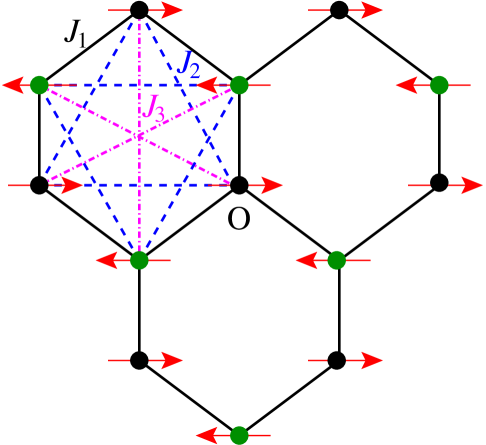
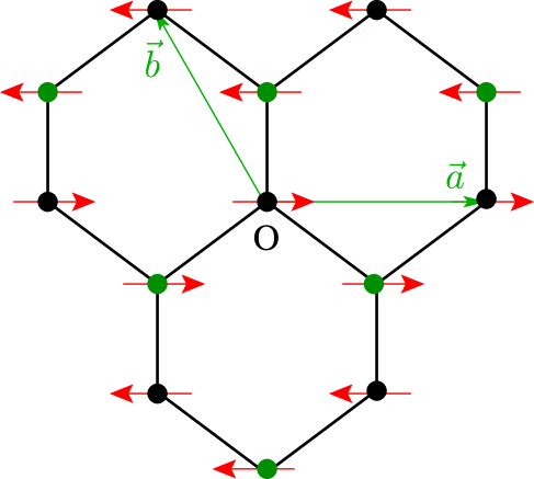
Figure 1: (Color online) The $J_{1}$–$J_{2}$–$J_{3}$ honeycomb model with $J_{1}>0;J_{2}>0;J_{3}>0$, showing (a) the bonds ($J_{1}=$ —– ; $J_{2}=---$ ; $J_{3}=-\cdot-$) and the Néel state, and (b) triangular Bravais lattice vectors $\mathbf{a}$ and $\mathbf{b}$ and one of the three equivalent striped states. Sites on sublattices ${\cal A}$ and ${\cal B}$ are shown by filled black and green circles respectively, and spins on the lattice are represented by the (red) arrows.

The fundamental low-energy parameter set that completely determines in this way the low-energy physics of magnetic systems comprises the GS energy per particle $E/N$, the average local on-site magnetization (viz., here the staggered magnetization) $M$ that plays the role of the order parameter, the zero-field (uniform, transverse) magnetic susceptibility $\chi$, the spin stiffness $\rho_{s}$, and the spin-wave velocity $c$. In previous studies Farnell et al. (2011); Li et al. (2012a); Bishop and Li (2012) of the spin-$\frac{1}{2}$ $J_{1}$–$J_{2}$–$J_{3}$ model on the honeycomb lattice along the particularly interesting line $J_{3}=J_{2}$, we have used the CCM implemented to high orders to give very accurate calculations for the quantities $E/N$ and $M$ in the magnetically ordered phases, and used them to investigate in detail the $T=0$ phase diagram of the model.

One of our aims here is to use the CCM now to directly calculate also the remaining low-energy parameters $\chi$ and $\rho_{s}$ (and hence also $\hbar c=\sqrt{\rho_{s}/\chi}$, with standard AFM hydrodynamics, and in units for $\chi$ where the gyromagnetic ratio $g\mu_{B}/\hbar=1$). Together with our earlier work, a knowledge of these quantities will provide a complete and consistent description of the model via low-energy $\chi$PT. Furthermore, as we shall see, the parameters $\chi$ and $\rho_{s}$ themselves provide further information on the $T=0$ phase structure of the model, both for the quantum critical points (QCPs) at which quasiclassical ordering melts, and also for the paramagnetic phases with no magnetic order into which the system passes. Finally, we also calculate the spin gap for the model, using the same CCM methodology, in an attempt to provide even more information about the model.

The plan of the remainder of the paper is as follows. In Sec. II we first describe the model itself, including its classical ($s\rightarrow\infty$) counterpart. The CCM technique is then briefly reviewed in Sec. III, where we concentrate on its key features, before presenting our detailed numerical results in Sec. IV. We end in Sec. V with a summary and conclusions.

II THE MODEL

The $J_{1}$–$J_{2}$–$J_{3}$ model on the honeycomb lattice is described by the Hamiltonian

$$H=J_{1}\sum_{\langle i,j\rangle}\mathbf{s}_{i}\cdot\mathbf{s}_{j}+J_{2}\sum_{\langle\langle i,k\rangle\rangle}\mathbf{s}_{i}\cdot\mathbf{s}_{k}+J_{3}\sum_{\langle\langle\langle i,l\rangle\rangle\rangle}\mathbf{s}_{i}\cdot\mathbf{s}_{l}\,,$$ (1)

in which the index $i$ runs over all $N$ lattice sites, and the indices $j$, $k$, and $l$ run respectively over all NN, NNN, and NNNN sites to $i$, and where in each sum each bond is counted once and once only. Each site $i$ of the lattice carries a spin-$\frac{1}{2}$ particle described by the spin operator ${\bf s}_{i}\equiv(s^{x}_{i},s^{y}_{i},s^{z}_{i})$. The lattice and the Heisenberg exchange bonds are illustrated in Fig. 1. In the present paper we will be interested in the case where each of the three types of bonds is AFM in nature, i.e., $J_{n}>0$; $n=1,2,3$.

The honeycomb lattice is bipartite with two triangular Bravais sublattices ${\cal A}$ and ${\cal B}$. If the lattice spacing on the honeycomb lattice (i.e., the distance between NN sites) is $d$, then sites on sublattice ${\cal A}$ are at positions $\mathbf{R}_{i}=m\mathbf{a}+n\mathbf{b}=\sqrt{3}(m-\frac{1}{2}n)d\hat{x}+\frac{3}{2}nd\hat{z}$, in terms of real-space basis vectors $\mathbf{a}=\sqrt{3}d\hat{x}$ and $\mathbf{b}=\frac{1}{2}d(-\sqrt{3}\hat{x}+3\hat{z})$ for the honeycomb lattice, which is defined to lie in the $xz$ plane, as shown in Fig. 1. Each unit cell $i$ at position vector $\mathbf{R}_{i}$ comprises a pair of sites, situated at $\mathbf{R}_{i}\in{\cal A}$ and $(\mathbf{R}_{i}+d\hat{z})\in{\cal B}$. The parallelogram formed by $\mathbf{a}$ and $\mathbf{b}$ defines the honeycomb Wigner-Seitz unit cell. The Wigner-Seitz cell may itself equivalently be taken as being centered on a point of sixfold symmetry so that it is bounded by the sides of a primitive hexagon of side $d$. The first Brillouin zone is then itself also a hexagon, which is rotated by 90^∘ with respect to the Wigner-Seitz hexagon, and which has a side of length $4\pi/(3\sqrt{3}d)$.

The classical version of the honeycomb model of Eq. (1) (i.e., when $s\rightarrow\infty$) has been studied by several authors Rastelli et al. (1979); Fouet et al. (2001); Mulder et al. (2010). For example, Rastelli et al. Rastelli et al. (1979) searched for coplanar or uniformly canted spin configurations that minimize the classical energy and found the former to be energetically favored. Generally they correspond to spiral configurations described by a wave vector Q, plus an angle $\theta$ that describes the relative orientation of the two spins in the same unit cell $i$, both of which are now characterized by the same triangular Bravais lattice vector $\mathbf{R}_{i}$. The classical spins (of length $s$) in unit cell $i$ are thus given by

$$\mathbf{s}_{i,\tau}=s[\cos(\mathbf{Q}\cdot\mathbf{R}_{i}+\theta_{\tau})\hat{x}_{s}+\sin(\mathbf{Q}\cdot\mathbf{R}_{i}+\theta_{\tau})\hat{z}_{s}]\,,$$ (2)

where $\hat{x}_{s}$ and $\hat{z}_{s}$ are two orthogonal unit vectors that define the plane of the spins in spin space, as shown in Fig. 1. The index $\tau$ labels the two sites in the unit cell. Clearly we may choose the angles $\theta_{\tau}$ so that $\theta_{A}=0$ for spins on sublattice ${\cal A}$ and $\theta_{B}=\theta$, say, for spins on sublattice ${\cal B}$.

In our regime of interest (i.e., when $J_{n}>0$; $n=1,2,3$) the classical model has a $(T=0)$ GS phase diagram comprising three distinct phases Fouet et al. (2001); Mulder et al. (2010). One value of the spiral wave vector that minimizes the classical GS energy is

$$\mathbf{Q}=\frac{2}{\sqrt{3}d}\cos^{-1}\left[\frac{J_{1}-2J_{2}}{4(J_{2}-J_{3})}\right]\hat{x}\,,$$ (3)

together with $\theta=\pi$. Clearly, the wave vector $\mathbf{Q}$ of Eq. (3) is only properly defined when

$$-1\leq\frac{J_{1}-2J_{2}}{4(J_{2}-J_{3})}\leq 1\,,$$ (4)

or, equivalently, when

$$y\leq\frac{3}{2}x-\frac{1}{4}\,;\quad y\leq\frac{1}{2}x+\frac{1}{4}\,,$$ (5)

where $x\equiv J_{2}/J_{1}$ and $y\equiv J_{3}/J_{1}$. The region in the positive quadrant (i.e., $x\geq 0$, $y\geq 0$) of the $xy$ plane that satisfies both inequalities of Eq. (5) is where the classical $J_{1}$–$J_{2}$–$J_{3}$ model on the honeycomb lattice has the spiral phase described by the wave vector $\mathbf{Q}$ of Eq. (3), and $\theta=\pi$, as the stable GS phase. Along the line $y=\frac{3}{2}x-\frac{1}{4}$, $\mathbf{Q}=\mathbf{\Gamma}\equiv(0,0)$, and the phase described by Eq. (2) simply becomes (continuously) the collinear Néel AFM phase illustrated in Fig. 1(a). The phase transition between the Néel and spiral phases is thus a continuous one. Similarly, along the line $y=\frac{1}{2}x+\frac{1}{4}$, $\mathbf{Q}=2\pi/(\sqrt{3}d)\hat{x}$, and the phase described by Eq. (2) becomes (continuously) the collinear striped AFM phase illustrated in Fig. 1(b). The phase transition between the striped and spiral phases is thus also a continuous one. The above two phase boundaries meet at the point $(x,y)=(\frac{1}{2},\frac{1}{2})$ which is the classical tricritical point. There is a first-order phase transition between the two collinear states (i.e., the Néel and striped states) along the boundary line $x=\frac{1}{2}$, for $y>\frac{1}{2}$. In summary, when $J_{1}>0$ and $x>0$, $y>0$, the classical $J_{1}$–$J_{2}$–$J_{3}$ model on the honeycomb lattice has three stable GS phases (at $T=0$): a Néel AFM phase for $y>\frac{3}{2}x-\frac{1}{4}$, $\frac{1}{6}<x<\frac{1}{2}$ and $y>0$, $0<x<\frac{1}{6}$; a striped AFM phase for $y>\frac{1}{2}x+\frac{1}{4}$, $x>\frac{1}{2}$; and a spiral phase for $0<y<\frac{3}{2}x-\frac{1}{4}$, $\frac{1}{6}<x<\frac{1}{2}$ and $0<y<\frac{1}{2}x+\frac{1}{4}$, $x>\frac{1}{2}$.

We note that the spiral and the striped states described by Eq. (3) and $\theta=\pi$ have two other similar states rotated by $\pm\frac{2\pi}{3}$ in the honeycomb plane. When $x\rightarrow\infty$ for a fixed finite value of $y$ (i.e., when the $J_{2}$ bond dominates), the spiral pitch angle $\phi=\cos^{-1}[\frac{1}{4}(J_{1}-2J_{2})/(J_{2}-J_{3})]\rightarrow\frac{2}{3}\pi$. In this limiting case the classical model thus becomes two HAFs on disconnected interpenetrating triangular lattices with the classical 3-sublattice Néel ordering of NN spins oriented at angle $\frac{2}{3}\pi$ to each other on each sublattice. In this limiting case the wave vector $\mathbf{Q}$ of Eq. (3) becomes one of the six corners of the first Brillouin zone, $\mathbf{K}^{(1)}=4\pi/(3\sqrt{3}d)\hat{x}$. Clearly, there are only two distinct such corner vectors, and these describe the two inequivalent 3-sublattice Néel orderings for a classical triangular HAF.

We also note that when the spiral pitch angle $\phi$ takes a value in the range $\frac{2}{3}\pi<\phi\leq\pi$ the wave vector $\mathbf{Q}$ of Eq. (3) lies outside the first Brillouin zone. It can equivalently be mapped back into the first Brillouin zone in this case, when $\mathbf{Q}$ moves continuously from a corner $\mathbf{K}^{(3)}=-2\pi/(3\sqrt{3}d)\hat{x}+2\pi/(3d)\hat{z}$ of the Brillouin zone along one of its edges to the midpoint $\mathbf{M}^{(2)}=2\pi/(3d)\hat{z}$. The striped state shown in Fig. 1(b) may thus be equivalently described by the ordering wave vector $\mathbf{Q}=\mathbf{M}^{(2)}$ (with the relative angle between sublattices ${\cal A}$ and ${\cal B}$ given by $\theta=\pi$). The other two striped states are thus given by the wave vectors of the two other inequivalent midpoints of edges of the first Brillouin zone, $\mathbf{M}^{(1)}=\pi/(\sqrt{3}d)\hat{x}+\pi/(3d)\hat{z}$ and $\mathbf{M}^{(3)}=-\pi/(\sqrt{3}d)\hat{x}+\pi/(3d)\hat{z}$ (and in both of these cases with $\theta=0$).

Although the spin ordering of Eq. (2) usually suffices to find all classical GS configurations Villain (1977), there is an assumption that the GS order is either unique (up to the trivial degeneracy associated with a global spin rotation) or exhibits, at most, a discrete degeneracy. However, exceptions can arise for special sets $\{\mathbf{Q}\}$ of wave vectors Fouet et al. (2001); Villain (1977). These include the case when $\mathbf{Q}$ is equal to one half or one quarter of a reciprocal lattice vector $\mathbf{G}$. This is precisely the case for the striped states where the wave vectors $\mathbf{Q}=\mathbf{M}^{(i)}$, $i=1,2,3$ are just one half of corresponding reciprocal lattice vectors. As explained by Fouet et al. Fouet et al. (2001) the GS ordering in this case spans a 2D manifold of non-planar GS configurations, all degenerate in energy.

It is well known that classical models that exhibit such an infinitely degenerate family (IDF) of GS phases in some region of the $T=0$ phase space often lead to the emergence of novel quantum phases in the corresponding quantum-mechanical model. A typical scenario then finds that quantum fluctuations lift this (accidental) GS degeneracy, either completely or in part by the well-known order by disorder mechanism Villain (1977); Villain et al. (1980); Shender (1982), so that just one or several members of the classical IDF are favored. Indeed, thermal or quantum fluctuations do select the collinear striped states out of the 2D IDF manifold, according to Ref. Fouet et al. (2001), wherein it is also explicitly shown in an ED study of the finite-lattice spectra that the degeneracy is lifted in favor of the collinear ordering.

In the extreme $s=\frac{1}{2}$ quantum limit one may also expect that quantum fluctuations might be strong enough to destroy any quasiclassical magnetic long-range order (LRO) completely in some region of the $T=0$ GS phase space. The goal of finding any such novel quantum phases with no magnetic LRO, and delimiting their region of stability in the $T=0$ phase space, has provided the impetus for much recent work Rastelli et al. (1979); Mattsson et al. (1994); Fouet et al. (2001); Mulder et al. (2010); Wang (2010); Cabra et al. (2011); Ganesh et al. (2011); Clark et al. (2011); Farnell et al. (2011); Reuther et al. (2011); Albuquerque et al. (2011); Mosadeq et al. (2011); Oitmaa and Singh (2011); Mezzacapo and Boninsegni (2012); Li et al. (2012a); Bishop et al. (2012); Bishop and Li (2012); Li et al. (2012b); Bishop et al. (2013); Ganesh et al. (2013); Zhu et al. (2013); Zhang and Lamas (2013); Gong et al. (2013); Yu et al. (2014) on the spin-$\frac{1}{2}$ $J_{1}$–$J_{2}$–$J_{3}$ model on the honeycomb lattice. A particularly challenging, yet potentially fruitful, regime is to consider the case $J_{3}=J_{2}\equiv\kappa J_{1}$ since it includes the point of maximum classical frustration, viz., the tricritical point at $\kappa=\kappa_{{\rm cl}}\equiv\frac{1}{2}$. Henceforth, therefore, we restrict ourselves to this regime.

In our earlier paper Farnell et al. (2011) we presented results for the GS energy and magnetic order parameter of the spin-$\frac{1}{2}$ $J_{1}$–$J_{2}$–$J_{3}$ model on the honeycomb lattice along the line $J_{3}=J_{2}\equiv\kappa J_{1}$, with $J_{1}>0$ and $\kappa>0$, using the CCM implemented in high orders. We found that the first-order transition in the classical ($s\rightarrow\infty$) model at $\kappa=\kappa_{{\rm cl}}\equiv\frac{1}{2}$ between the Néel and collinear striped AFM phases is split into two transitions for the $s=\frac{1}{2}$ model. The Néel phase was found to survive for $\kappa<\kappa_{c_{1}}\approx 0.47$, and the striped phase for $\kappa>\kappa_{c_{2}}\approx 0.60$. In the region $\kappa_{c_{1}}<\kappa<\kappa_{c_{2}}$ between the two quasiclassical phases we found a paramagnetic phase with no discernible magnetic order. By further calculating within the same CCM methodology, the susceptibilities of the two AFM phases against the formation of a state with plaquette valence-bond crystalline (PVBC) order, we concluded that the intermediate state was one with PVBC order. The evidence from those calculations was that the quantum phase transition (QPT) at $\kappa_{c_{2}}$ appears to be a first-order one, while that at $\kappa_{c_{1}}$ is of continuous type. Since the Néel and PVBC phases break different symmetries, we concluded that the quantum transition at $\kappa_{c_{1}}$ between these two phases is of the deconfined type Senthil et al. (2004a); *Senthil:2004_PRB_deconfinedQC.

Our aim in the present paper is to shed further light on the model by calculating other physical properties within the same CCM methodology as used previously. Firstly, in order to gain more evidence about the nature of the intermediate phase we calculate the spin gap, i.e., the energy gap between the ground state and the lowest-lying (magnon) triplet excitation. Secondly, as discussed previously, we also calculate for both quasiclassical phases the spin stiffness, $\rho_{s}$, and the zero-field (uniform, transverse) magnetic susceptibility, $\chi$, in order both to provide a complete set of low-energy parameters for both phases of the model and to use these parameters to provide more numerical evidence for the two QPTs at $\kappa_{c_{1}}$ and $\kappa_{c_{2}}$.

The spin stiffness (or helicity modulus) of a spin-lattice system is a measure of the energy required to rotate the order parameter of a magnetically ordered thermodynamic system by an (infinitesimal) angle $\theta$ per unit length in a given direction. Thus, if $E(\theta)$ is the GS energy as a function of the imposed twist and $N$ is the number of lattice sites, we have

$$\frac{E(\theta)}{N}=\frac{E(\theta=0)}{N}+\frac{1}{2}\rho_{s}\theta^{2}+O(\theta^{4})\,.$$ (6)

Note that $\theta$ has the dimensions of an inverse length. In the thermodynamic limit ($N\rightarrow\infty$) a nonzero (positive) value of $\rho_{s}$ implies that the system has magnetic long-range order (LRO), while the magnetic LRO melts at the point where $\rho_{s}\rightarrow 0$. Clearly, for the Néel AFM state of Fig. 1(a), for which the ordering wave vector $\mathbf{Q}=\mathbf{\Gamma}=(0,0)$, the quantity $\rho_{s}$ is independent of the direction of the applied twist, whereas for the particular striped AFM state shown in Fig. 1(b), for which $\mathbf{Q}=2\pi/(\sqrt{3}d)\hat{x}$, the physically relevant direction in which to apply the twist is the $x$ direction. Figure 2 thus illustrates the two twisted AFM states (i.e., the Néel and striped states) used in our calculations for the spin stiffness coefficient.

 

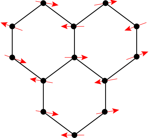
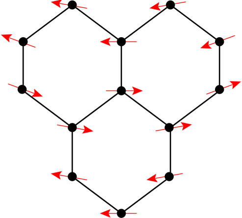
Figure 2: (Color online) The twisted reference states for the calculation of the spin stiffness coefficient, $\rho_{s}$, for the $J_{1}$–$J_{2}$–$J_{3}$ honeycomb model, showing the twist applied in the $x$ direction to the (a) Néel and (b) striped states. The spins on lattice sites •  are represented by the (red) arrows.

The definition of Eq. (6) easily leads to the corresponding values of $\rho_{s}$ for the classical $(s\rightarrow\infty)$ $J_{1}$–$J_{2}$–$J_{3}$ model on the honeycomb lattice,

$$\rho^{{\rm N\acute{e}el}}_{s;\,{\rm cl}}=\frac{3}{4}(J_{1}-6J_{2}+4J_{3})d^{2}s^{2}\,,$$ (7)

and

$$\rho^{{\rm striped}}_{s;\,{\rm cl}}=\frac{3}{4}(-J_{1}-2J_{2}+4J_{3})d^{2}s^{2}\,.$$ (8)

The lines along which the spin stiffness coefficients given by Eqs. (7) and (8) vanish are, as expected, just the classical phase boundaries for the two AFM states with the spiral state.

It is also interesting to note that in the limiting case $J_{3}\rightarrow\infty$, for fixed values of $J_{1}$ and $J_{2}$, the $J_{1}$–$J_{2}$–$J_{3}$ model reduces to four decoupled honeycomb-lattice HAFs, each with NN coupling $J_{3}$ and lattice spacing 2$d$. Thus, the GS energy in the case $\{J_{1}=0,\,J_{2}=0,\,J_{3}=1\}$ should be equal to that of the case when $\{J_{1}=1,\,J_{2}=0,\,J_{3}=0\}$. Similarly, the spin stiffness in the former limit should equal four times that in the latter limit, due to the doubling of the lattice size of each of the four decoupled honeycomb sublattices. Just, as this result holds for the classical model ($s\rightarrow\infty$), from Eq. (7), so it should also hold for general values of the spin quantum number $s$.

In order to calculate the zero-field magnetic susceptibility, $\chi$, we now place our system in an external transverse magnetic field $\mathbf{h}$. For the two collinear AFM states shown in Fig. 1, both with spins aligned along the $x_{s}$ direction, we apply the field in the $z_{s}$ direction, $\mathbf{h}=h\hat{z_{s}}$. The Hamiltonian $H=H(h=0)$ of Eq. (1) thus becomes

$$H(h)=H(h=0)+h\sum_{l}s^{z}_{l}\,,$$ (9)

in units where the gyromagnetic ratio $g\mu_{B}/\hbar=1$. In the presence of the field, the spins will now cant at an angle $\alpha$ to the $x_{s}$ axis with respect to their zero-field configurations, as shown in Fig. 3 for the two classical AFM states illustrated in Fig.1.

 

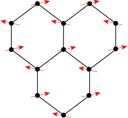
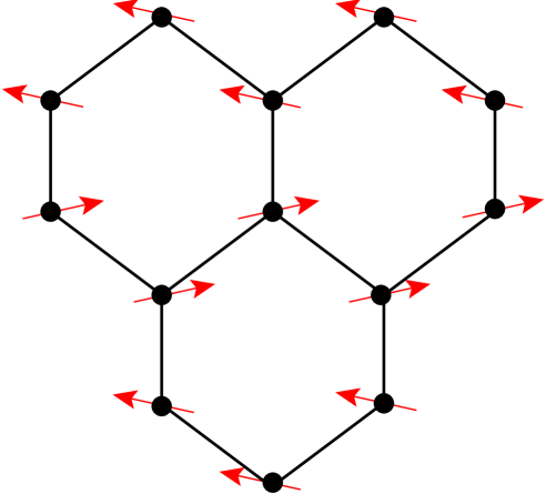
Figure 3: (Color online) The canted reference states for the calculation of the zero-field magnetic susceptibility, $\chi$, for the $J_{1}$–$J_{2}$–$J_{3}$ honeycomb model. The external magnetic field is applied in the $z_{s}$ direction to the (a) Néel and (b) striped states, shown in Fig. 1. The spins on lattice sites •  are represented by the (red) arrows.

The classical ($s\rightarrow\infty$) value of $\alpha$ for each of the states is easily calculated by minimizing the classical energy, $E=E(h)$, corresponding to Eq. (9) with respect to $\alpha$. The uniform magnetic susceptibility is then defined, as usual, by

$$\chi({h})=-\frac{1}{N}\frac{{\rm d}^{2}E}{{\rm d}h^{2}}\,,$$ (10)

and its zero-field limit as $\chi\equiv\chi(0)$. The corresponding analog of Eq. (6) is thus,

$$\frac{E(h)}{N}=\frac{E(h=0)}{N}-\frac{1}{2}\chi h^{2}+O(h^{4})\,.$$ (11)

These relations readily yield the values of $\chi$ for the two collinear AFM states of the classical ($s\rightarrow\infty$) $J_{1}$–$J_{2}$–$J_{3}$ model on the honeycomb lattice,

$$\chi^{{\rm N\acute{e}el}}_{{\rm cl}}=\frac{1}{6(J_{1}+J_{3})}\,,$$ (12)

and

$$\chi^{{\rm striped}}_{{\rm cl}}=\frac{1}{2(J_{1}+4J_{2}+3J_{3})}\,,$$ (13)

with both parameters independent of $s$ in the classical case. The two values of $\chi$ become equal (but nonzero, note) along the line $J_{2}=\frac{1}{2}J_{1}$ (independent of $J_{3}$), which is the classical phase boundary between the two AFM states.

We note that our definitions for both $\rho_{s}$ and $\chi$ are per unit site, as is more usual for a discrete lattice description. On the other hand, in continuum field-theoretic terms, such as in descriptions using $\chi$PT, it is more natural to define corresponding quantities, $\bar{\rho_{s}}$ and $\bar{\chi}$, per unit area. Since the honeycomb lattice has $4/(3\sqrt{3}d^{2})$ sites per unit area, $\rho_{s}=\frac{3}{4}\sqrt{3}d^{2}\bar{\rho_{s}}$ and $\chi=\frac{3}{4}\sqrt{3}d^{2}\bar{\chi}$.

III THE COUPLED CLUSTER METHOD

The CCM is one of only a very few universal methods of ab initio quantum many-body theory (QMBT) that are capable of systematic improvement in well-defined hierarchies of approximations. It is nowadays one of the most pervasive, most powerful, and most accurate at attainable levels of computational implementation, of all fully microscopic formulations of QMBT. It has been applied with considerable success to a wide range of physical systems Bishop and Kümmel (1987); Bartlett (1989); Arponen and Bishop (1991); Bishop (1991, 1998), ranging from the electron gas to atoms and molecules of interest in quantum chemistry, from nuclear matter and finite atomic nuclei to strongly interacting quantum field theories, and from models in quantum optics, quantum electronics, and solid state optoelectronics to diverse condensed matter systems. The CCM has thus yielded accurate numerical results for a very wide range of both finite and extended systems defined either in a spatial continuum or on a regular discrete lattice. Of particular relevance to the present paper is the fact that the method has already been applied with demonstrable success to a large number of spin-lattice problems of interest in quantum magnetism (and see, e.g., Refs. Bishop and Rosenfeld (1998); Farnell et al. (2014, 2011); Li et al. (2012a); Bishop et al. (2012); Bishop and Li (2012); Li et al. (2012b); Bishop et al. (2013); Roger and Hetherington (1990); Bishop et al. (1992); Zeng et al. (1998); Farnell and Bishop (2004); Krüger et al. (2006); Darradi et al. (2008); Farnell et al. (2009); Götze et al. (2011); Bishop et al. (2014); Li et al. (2015); Richter et al. (2015) and references cited therein).

Two characteristic and rather unique features of the CCM that are immediately worthy of mention are: (i) its ability to deal with infinite ($N\rightarrow\infty$) systems from the outset, hence obviating the need for any finite-size scaling, which is required in most competing methods; and (ii) the fact that it exactly preserves the important Hellmann-Feynman theorem at all levels of approximate implementation. The method is implemented in practice, as we explain below, at various levels of approximation in a well-defined truncation hierarchy, with each level specified by a truncation index $n=1,2,3,\cdots$. The only approximation made is then to extrapolate the values obtained for the physical observables at the $n$th level to the $n\rightarrow\infty$ limit where the CCM becomes exact.

The CCM has been described in detail in earlier papers (and see, e.g., Refs. Arponen and Bishop (1991); Bishop (1998, 1991); Bishop et al. (1992); Zeng et al. (1998); Farnell et al. (2014); Bishop et al. (2014); Li et al. (2015) and references cited therein), and hence we briefly outline only its most salient features here. Every implementation of the method begins with the choice of a suitable normalized reference (or model) state, with respect to which the quantum correlations present in the exact GS phase under study can then be incorporated at the next stage. For this study suitable choices of the model state $|\Phi\rangle$ will be the two quasiclassical AFM states (viz., the Néel and collinear striped states) shown in Figs. 1(a) and 1(b).

The exact GS ket- and bra-state wave functions, which satisfy the respective Schrödinger equations,

$$H|\Psi\rangle=E|\Psi\rangle\,;\quad\langle\tilde{\Psi}|H=E\langle\tilde{\Psi}|\,,$$ (14)

are chosen to have normalization conditions such that $\langle\tilde{\Psi}|\Psi\rangle=\langle{\Phi}|\Psi\rangle=\langle{\Phi}|\Phi\rangle=1$. These exact states are then parametrized in terms of the respective model state as

$$|\Psi\rangle=e^{S}|\Phi\rangle\,;\quad\langle\tilde{\Psi}|=\langle\Phi|\tilde{S}e^{-S}\,,$$ (15)

with the exponential parametrization being a key characteristic feature of the CCM. The two correlation operators are then themselves formally decomposed as

$$S=\sum_{I\neq 0}{\cal S}_{I}C^{+}_{I}\,;\quad\tilde{S}=1+\sum_{I\neq 0}\tilde{{\cal S}}_{I}C^{-}_{I}\,,$$ (16)

where we define $C^{+}_{0}\equiv 1$ to be the identity operator, and where the set index $I$ denotes a complete set of single-particle configurations for all of the particles. In our present spin-lattice application it defines a specific multispin-flip configuration with respect to the model state $|\Phi\rangle$, such that $C^{+}_{I}|\Phi\rangle$ is the corresponding wave function for this configuration of spins. The model state $|\Phi\rangle$ thus acts as s fiducial (or cyclic) vector or, in other words, as a generalized vacuum state, with respect to the complete set of mutually commuting creation operators $\{C^{+}_{I}\}$, and which hence satisfy the conditions $\langle\Phi|C^{+}_{I}=0=C^{-}_{I}|\Phi\rangle\,,\quad\forall I\neq 0$, where the destruction operators $C^{-}_{I}\equiv(C^{+}_{I})^{\dagger}$.

It is very convenient for spin-lattice problems to consider each lattice site $i$ as totally equivalent to all others, whatever the choice of model state $|\Phi\rangle$, and one simple way to do this is to make a passive rotation of each spin so that in its own local spin-coordinate frame it points, say, in the downward (i.e., negative $z_{s}$) direction as in the spin coordinate frame shown in Fig. 1. Such choices of local spin coordinates clearly do not affect the basic SU(2) spin commutation relations. However, all independent-spin product model states now take the universal form $|\Phi\rangle=|\downarrow\downarrow\downarrow\cdots\downarrow\rangle$. Thus, $C^{+}_{I}$ can simply be expressed as a product of single-spin raising operators, $s^{+}_{k}\equiv s^{x}_{k}+is^{y}_{k}$, such that $C^{+}_{I}\equiv s^{+}_{k_{1}}s^{+}_{k_{2}}\cdots s^{+}_{k_{n}};\;n=1,2,\cdots,2sN$. For the present study, where we consider $s=\frac{1}{2}$, each site index included in the corresponding set index $I\equiv\{k_{1},k_{2},\cdots,k_{n};\;n=1,2,\cdots,2sN\}$ may appear no more than once. Once the local spin coordinates have been chosen for the particular model state $|\Phi\rangle$, the Hamiltonian $H$ simply needs to be re-expressed in terms of them.

In principle, what remains is then to calculate the CCM correlation coefficients $\{{\cal S}_{I},\tilde{{\cal S}}_{I}\}$. This is achieved by minimization of the GS energy expectation functional,

$$\bar{H}=\bar{H}[{\cal S}_{I},{\tilde{\cal S}_{I}}]\equiv\langle\Phi|\tilde{S}e^{-S}He^{S}|\Phi\rangle\,,$$ (17)

with respect to each of the coefficients $\{{\cal S}_{I},{\tilde{\cal S}}_{I}\,;\forall I\neq 0\}$. From Eqs. (16) and (17), variation with respect to ${\tilde{\cal S}}_{I}$ yields the coupled set of non-linear equations,

$$\langle\Phi|C^{-}_{I}e^{-S}He^{S}|\Phi\rangle=0\,,\quad\forall I\neq 0\,,$$ (18)

for the coefficients $\{{\cal S}_{I}\}$. Similarly, variation of Eq. (17) with respect to ${\cal S}_{I}$ yields the corresponding set of linear equations

$$\langle\Phi|\tilde{S}e^{-S}[H,C^{+}_{I}]e^{S}|\Phi\rangle=0\,,\quad\forall I\neq 0\,,$$ (19)

for the coefficients $\{{\tilde{{\cal S}}}_{I}\}$, once Eq. (18) has been solved for the coefficients $\{{\cal S}_{I}\}$. The GS energy eigenvalue $E$, which is the value of $\bar{H}$ at the minimum, is then simply

$$E=\langle\Phi|e^{-S}He^{S}|\Phi\rangle=\langle\Phi|He^{S}|\Phi\rangle\,.$$ (20)

Equation (19) may then be written in the equivalent form,

$$\langle\Phi|\tilde{S}(e^{-S}He^{S}-E)C^{+}_{I}|\Phi\rangle=0\,,\quad\forall I\neq 0\,,$$ (21)

of a set of generalized linear eigenvalue equations for the coefficients $\{\tilde{\cal S}_{I}\}$.

Having built in the correlations into our CCM parametrization of the GS wave function $|\Psi\rangle$, it now suffices to apply a linear excitation operator $X^{e}$ to $|\Psi\rangle$ to parametrize the excited-state wave function $|\Psi_{e}\rangle$ as

$$|\Psi_{e}\rangle=X^{e}e^{S}|\Phi\rangle\,,\quad X^{e}=\sum_{I\neq 0}{\cal X}^{e}_{I}C^{+}_{I}\,.$$ (22)

By suitably combining the GS Schrödinger equation (14) with its excited-state counterpart,

$$H|\Psi_{e}\rangle=E_{e}|\Psi\rangle\,,$$ (23)

and realizing that the operators $X^{e}$ and $S$ commute, by construction, we readily deduce the equation,

$$e^{-S}[H,X^{e}]e^{S}|\Phi\rangle=\Delta_{e}X^{e}|\Phi\rangle\,,$$ (24)

where $\Delta_{e}\equiv E_{e}-E$ is the excitation energy. By taking the overlap of Eq. (24) with the state $\langle\Phi|C^{-}_{I}$ we find

$$\langle\Phi|C^{-}_{I}e^{-S}[H,X^{e}]e^{S}|\Phi\rangle=\Delta_{e}{{\cal X}}^{e}_{I}\,,\quad\forall I\neq 0\,,$$ (25)

when the states labelled by the indices $\{I\}$ are, as usual, orthonormalized, $\langle\Phi|C^{-}_{I}C^{+}_{J}|\Phi\rangle=\delta(I,J)$. The generalized eigenvalue equation (25) is then solved for $\Delta_{e}$.

In the present case the configurations chosen in the expansion of Eq. (22) for the excitation operator $X^{e}$ are restricted to those that change the $z$ component of the total spin, $S^{z}_{T}$, by one. The value we thus obtain for $\Delta_{e}$ is then the spin-triplet gap, which we henceforth denote as $\Delta$.

Up to this point no approximations have been made. Nevertheless, the equations (18) for the coefficients $\{{\cal S}_{I}\}$ are intrinsically nonlinear and one may wonder if truncations are needed in the evaluation of the exponential functions. We note that these appear, however, only in the combination of the similarity transform $e^{-S}He^{S}$ of the Hamiltonian, which may be expanded in terms of the well-known nested commutator sum. Another key feature of the CCM is that this otherwise infinite sum now actually terminates exactly with the double commutator term. This is due to the basic SU(2) commutation relations and because all of the terms in Eq. (16) comprising $S$ commute with one another and are simple products of spin-raising operators. All terms in the expansion of $e^{-S}He^{S}$ are thus linked, and the Goldstone linked cluster theorem is exactly preserved, even if the expansion of Eq. (16) is truncated in any way, thereby guaranteeing size-extensivity at any such level of truncation and our ability to work from the outset in the thermodynamic ($N\rightarrow\infty$) limit. Similar considerations also apply to Eqs. (19) and (25).

Thus, the only approximation made in practice for the GS calculation is to restrict the set of indices $\{I\}$ retained in the expansions of Eq. (16) for the operators $\{S,\tilde{S}\}$. Here we utilize the well-tested localized (lattice-animal-based subsystem) LSUB$n$ scheme used in our earlier work on this model Farnell et al. (2011); Li et al. (2012a); Bishop and Li (2012) and in many other studies too. The LSUB$n$ scheme is defined so that at the $n$th level of approximation we retain all multispin-flip configurations $\{I\}$ in Eq. (16) that are defined over $n$ or fewer contiguous lattice sites. Such cluster configurations are said to be contiguous in this sense if every site in the cluster is NN to at least one other. The number, $N_{f}=N_{f}(n)$, of such distinct fundamental configurations may be reduced by utilizing the space- and point-group symmetries of the model, together with any conservation laws that pertain to both the Hamiltonian and the specific model state being used. Even so, the number $N_{f}(n)$ increases rapidly as the truncation index $n$ is increased, and the need eventually arises to use massive parallelization together with supercomputing resources for the highest-order calculations Zeng et al. (1998); ccm .

For the excited-state calculation of the spin gap $\Delta$ the choice of clusters for the excitation operator $X^{e}$ which are retained in Eq. (22) is different from that of the GS, since we restrict ourselves now to those that change the $z$ component, $S^{z}$, of total spin by one unit. Nevertheless, we use the same LSUB$n$ scheme for both the GS and excited-state calculations, thereby ensuring comparable accuracy for both. The number $N_{f}=N_{f}(n)$ at a given level $n$ of truncation is appreciably higher for the excited-state than for the corresponding GS calculation. Nevertheless the corresponding CCM equations have been solved for the present model using both quasiclassical (Néel and striped) AFM states as model states in LSUB$n$ approximations with $n\leq 12$.

Clearly, the CCM LSUB$n$ approximations become exact, by construction, in the $n\rightarrow\infty$ limit. There exist well-tested, accurate extrapolation rules for the GS quantities $E/N$ and $M$, as we have described and used in our earlier paper Farnell et al. (2011) for this model. Similarly, for the spin gap, we use the extrapolation scheme Richter et al. (2015); Krüger et al. (2000),

$$\Delta(n)=d_{0}+d_{1}n^{-1}+d_{2}n^{-2}\,,$$ (26)

to obtain the extrapolated value $\Delta\equiv\Delta(\infty)=d_{0}$ from the CCM LSUB$n$ approximations, $\Delta(n)$. Similar schemes have also been successfully used previously for both the spin stiffness $\rho_{s}$ Krüger et al. (2006); Darradi et al. (2008),

$$\rho_{s}(n)=s_{0}+s_{1}n^{-1}+s_{2}n^{-2}\,,$$ (27)

and the zero-field magnetic susceptibility, $\chi$ Darradi et al. (2008); Farnell et al. (2009),

$$\chi(n)=x_{0}+x_{1}n^{-1}+x_{2}n^{-2}\,.$$ (28)

In the latter case, as a check on the validity and accuracy of the scheme, we also utilize the completely unbiased scheme,

$$\chi(n)=\bar{x}_{0}+\bar{x}_{1}n^{-\nu}\,,$$ (29)

in which the leading exponent $\nu$ is itself a fitting parameter, along with $\bar{x}_{0}$ and $\bar{x}_{1}$. Finally, since the lowest-order LSUB$n$ approximants (particularly that with $n=2$) are less likely to conform well to these extrapolation rules than those with higher values of $n$, and also since the hexagon is the fundamental structural element of the honeycomb lattice, we prefer to use LSUB$n$ data with $n\geq 6$, whenever practicable, to perform each of the extrapolations in practice.

IV RESULTS

In our earlier work on the spin-$\frac{1}{2}$ $J_{1}$–$J_{2}$–$J_{3}$ model on the honeycomb lattice along the line $J_{3}=J_{2}$ $(=\kappa J_{1})$ in phase space Farnell et al. (2011) we employed the CCM and computed LSUB$n$ results for both the GS energy per spin, $E/N$, and magnetic order parameter, $M$, with values of the truncation index $n\leq 12$, using both the Néel and striped collinear AFM states as CCM model states. Although the number of fundamental configurations, $N_{f}$, at a given LSUB$n$ level of approximation is greater for the triplet excited state than for the ground state for the corresponding CCM calculations based on both model states, we are still able to calculate the spin gap $\Delta$ at LSUB$n$ levels with $n\leq 12$, even with the increased computational difficulty. We are thus able to achieve comparable accuracy for both the ground and excited states.

We show in Fig. 4(a) our “raw” LSUB$n$ results for the spin gap $\Delta$ with $n=\{6,8,10,12\}$, based on both the Néel and striped collinear states used separately as the CCM model state.

 

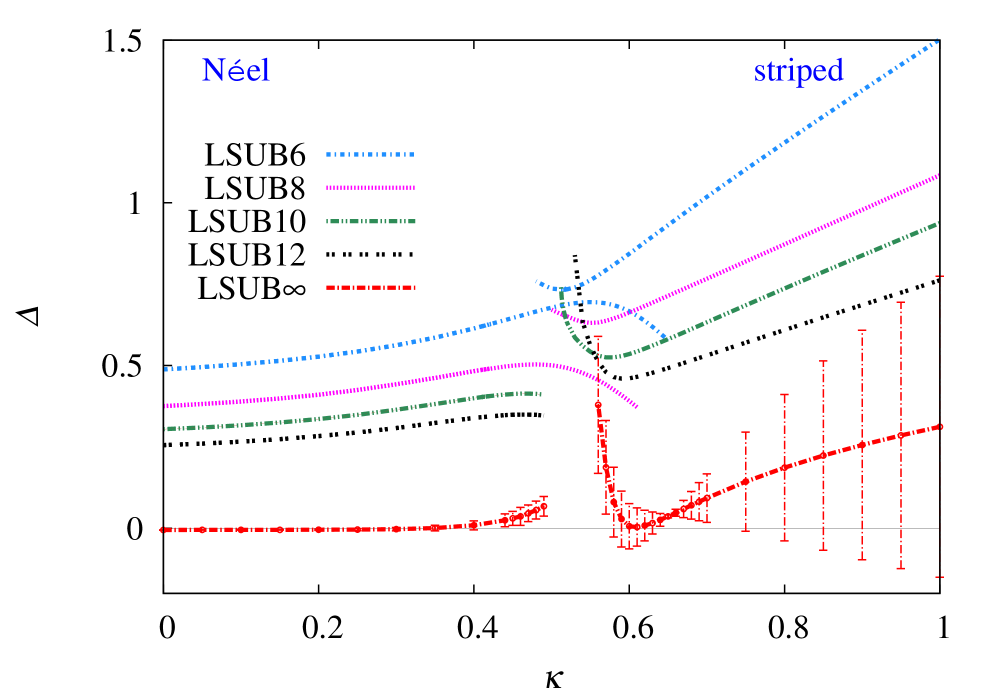
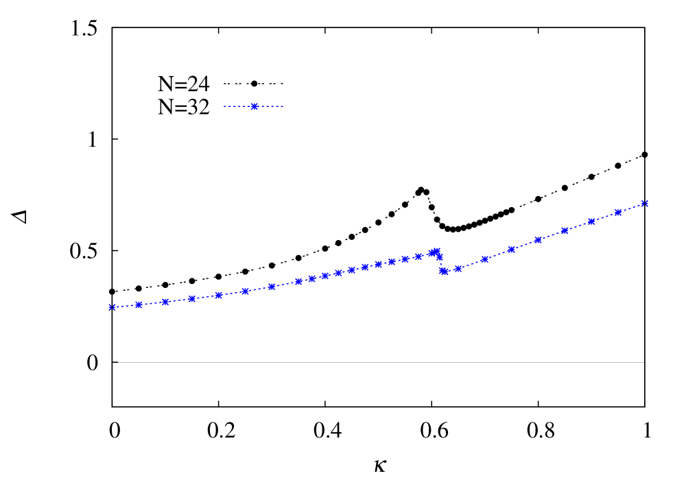
Figure 4: (Color online) The spin gap $\Delta$ versus the frustration parameter $\kappa\equiv J_{2}/J_{1}$, for the spin-$\frac{1}{2}$ $J_{1}$–$J_{2}$–$J_{3}$ model on the honeycomb lattice (with $J_{1}=1$, $J_{3}=J_{2}>0$). (a) CCM results based on the Néel and the striped AFM states as CCM model states. The LSUB$n$ results are shown with $n=\{6,8,10,12\}$. The extrapolated LSUB$\infty$ results using Eq. (26) are shown, together with the error bars associated with the fit. (b) ED results for lattices with $N=24$ and $N=32$ spins.

We also show the corresponding (LSUB$\infty$) extrapolated values, as obtained using the scheme of Eq. (26). For the Néel results our method of solution is as follows. We first solve for the pure Heisenberg AFM in the case $\kappa=0$, where we find a stable physical solution to the CCM equations at each LSUB$n$ level of truncation. For a given value of the truncation index $n$ the corresponding LSUB$n$ solution is tracked as the frustration parameter $\kappa$ is increased incrementally, just to the point where this stable solution terminates, as shown in Fig. 4(a). These termination points for the excited-state CCM equations are completely analogous to those also found for the GS CCM equations, which have been well described and documented previously (see, e.g., Refs. Bishop et al. (2012, 2013); Farnell and Bishop (2004); Bishop et al. (2014)). They are direct manifestations of the respective QCP in the physical system under study, at which the corresponding form of magnetic order in the associated model state melts. As is usually the case, we find that each LSUB$n$ Néel solution with a fixed (finite) value of $n$ terminates at a higher value of $\kappa$ than the corresponding actual critical value, $\kappa_{c_{1}}$, which is just the LSUB$\infty$ limiting value. The outcome is that we may thereby consider a range for the parameter $\kappa$ that is appreciably beyond the (seemingly continuous) transition at $\kappa_{c_{1}}$ from the Néel phase to the quantum paramagnetic phase.

On the other side of the phase diagram we similarly track each LSUB$n$ solution based on the collinear striped state as CCM model state from high values of $\kappa$ down to some respective lower transition point, corresponding to the actual transition at $\kappa_{c_{2}}$. Again, for each value of the transition index $n$, we may enter into the region below the (seemingly first-order) transition at $\kappa_{c_{2}}$ into the quantum paramagnetic phase. Of course, if the transition at $\kappa_{c_{2}}$ is indeed of first-order type, as seems likely from all prior available evidence, one might possibly query the validity of our CCM results based on the striped collinear state in the region $\kappa<\kappa_{c_{2}}$.

In Fig. 4(a) for the LSUB$\infty$ extrapolated values of $\Delta$ based on our LSUB$n$ results with $n=\{6,8,10,12\}$, we also show the error bars associated with the assumed scheme of Eq. (26). It is clear that the fit on the Néel side of the phase diagram is markedly better than that on the striped collinear side. Very interestingly, very similar behavior was also observed in a recent CCM study of the spin gap in the spin-$\frac{1}{2}$ $J_{1}$–$J_{2}$ model on the square lattice Richter et al. (2015), where possible reasons for the difference in accuracy of the fits for small and large values of $\kappa$ were discussed. Despite this difference in the quality of the extrapolations for the Néel and striped phases, the results in Fig. 4(a) are clearly compatible with $\Delta$ being zero in the ranges $\kappa<\kappa_{c_{1}}$ and $\kappa>\kappa_{c_{2}}$ for the two quasiclassical GS phases with magnetic LRO, where the spin gap must be zero.

Conversely, we see from Fig. 4(a) that $\Delta>0$ for a considerable range of values in the range $\kappa_{c_{1}}<\kappa<\kappa_{c_{2}}$ on both the Néel $(\kappa>\kappa_{c_{1}})$ and striped $(\kappa<\kappa_{c_{2}})$ sides of the region, over which the LSUB$n$ solutions with $n\leq 12$ persist, before their respective termination points. The values of $\kappa$ at which the LSUB$\infty$ curves for $\Delta$ become nonzero are also completely compatible with the values for $\kappa_{c_{1}}$ and $\kappa_{c_{2}}$ determined by us previously Farnell et al. (2011), at which the magnetic order parameter vanishes, $M\rightarrow 0$. Our results are incompatible with the entire intermediate phase for $\kappa_{c_{1}}<\kappa<\kappa_{c_{2}}$ being a gapless spin liquid. By contrast they provide supporting evidence to our earlier findings Farnell et al. (2011) that the quantum paramagnetic phase in this regime has PVBC order. On the other hand, our results for $\Delta$ would not, by themselves, rule out a gapped spin liquid in the intermediate regime.

It is interesting to note that our results for $\Delta$ being nonzero over (at least part of) the intermediate regime for the present honeycomb model, are in contrast to the equivalent CCM results Richter et al. (2015) for the corresponding intermediate quantum paramagnetic regime in the spin-$\frac{1}{2}$ $J_{1}$–$J_{2}$ model on the square lattice. For the latter case the extrapolated values of $\Delta$ over the entire parameter region accessible were found to be zero (or very close to zero). For the spin-$\frac{1}{2}$ $J_{1}$–$J_{2}$ model on the square lattice the Néel order is found to melt at a comparable value of the frustration parameter, $\kappa\equiv J_{2}/J_{1}$, at $\kappa_{c_{1}}\approx 0.45$, with a paramagnetic state in the region $\kappa_{c_{1}}<\kappa<\kappa_{c_{2}}\approx 0.59$. In this case the CCM based on the Néel state as model state can access the region $\kappa_{c_{1}}<\kappa\lesssim 0.49$ in LSUB$n$ approximations with $n\leq 12$ Richter et al. (2015), and in this region around the seemingly continuous transition at $\kappa_{c_{1}}$ the extrapolated CCM value of $\Delta$ is zero within computational accuracy. A very recent, accurate, density-matrix renormalization group calculation Gong et al. (2014) also finds good evidence for a near-critical state in the region $\kappa_{c_{1}}<\kappa\lesssim 0.5$, with a very small gap for the finite-sized systems studied, and also for a gapped PVBC state in the remainder of the paramagnetic regime, $0.5\lesssim\kappa<\kappa_{c_{2}}$.

Finally, on the issue of the spin gap, we also present corresponding results in Fig. 4(b) for the current model obtained by ED, for lattices containing $N=24,32$ spins. Clearly, neither lattice is large enough to show clearly the $N\rightarrow\infty$ behavior of $\Delta=0$ over both quasiclassical regimes (i.e., Néel and striped collinear). Nevertheless, there is evidence (interestingly, more marked for the smaller lattice) of a gap opening up around $\kappa\approx 0.6$ (i.e., at $\kappa_{c_{2}}$) as $\kappa$ is decreased from above. The steep decay around this value (seen most clearly in the $N=32$ data) is due to a level crossing in the triplet state. While the ED data are clearly indicating the first-order transition at $\kappa=\kappa_{c_{2}}$, they are, unsurprisingly, quite smooth around the continuous transition at $\kappa=\kappa_{c_{1}}$. Thus, while the ED results certainly do not contradict our CCM results, by themselves they are certainly much less predictive than the corresponding CCM results. Certainly, they do not, by themselves, contradict the appearance of a gap in the intermediate regime $\kappa_{c_{1}}<\kappa<\kappa_{c_{2}}$ with a sizable peak value, $\Delta\approx 0.4$, as shown by the CCM results.

We turn now to our results for the low-energy parameters, $\rho_{s}$ and $\chi$. In view of the lower symmetries of the twisted and canted CCM model states used respectively for these parameters, as illustrated in Figs. 2 and 3, the numbers $N_{f}$ of fundamental configurations at a given LSUB$n$ level of approximation are greater than those for the GS parameters $E/N$ and $M$ and for the spin gap $\Delta$. For example, for the calculation of $\Delta$, $N_{f}\approx 10^{4}\,(2\times 10^{5})$ for LSUB$n$ approximations based on the Néel model state with $n=10\,(12)$. Corresponding values based on the striped model state are $N_{f}\approx 2.5\times 10^{4}\,(5\times 10^{5})$ with $n=10\,(12)$. By contrast, for the twisted model states used for the calculation of $\rho_{s}$, as shown in Fig. 2, $N_{f}\approx 3.5\times 10^{5}$ at the LSUB10 level of approximation, and it becomes computationally infeasible to perform LSUB$n$ calculation for $\rho_{s}$ at higher truncation levels, $n\geq 12$.

Figure 5 shows our “raw” CCM LSUB$n$ results with $n=\{6,8,10\}$ for $\rho_{s}$, together with the corresponding LSUB$\infty$ values using the extrapolation scheme of Eq. (27) together with this data set.

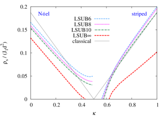
Figure 5: (Color online) CCM results for the spin stiffness $\rho_{s}$ (in units of $J_{1}d^{2}$) versus the frustration parameter $\kappa\equiv J_{2}/J_{1}$, for the spin-$\frac{1}{2}$ $J_{1}$–$J_{2}$–$J_{3}$ model on the honeycomb lattice (with $J_{1}=1$, $J_{3}=J_{2}>0$). We show results based on the Néel AFM and the striped AFM states as CCM model states. The LSUB$n$ results are shown with $n=\{6,8,10\}$, together with the extrapolated LSUB$\infty$ results using Eq. (27) with this data set. The classical results from Eqs. (7) and (8) are also shown for the value $s=\frac{1}{2}$.

For comparison purposes, we also show in Fig. 5 the corresponding classical values obtained from Eqs. (7) and (8) by putting $J_{3}=J_{2}=\kappa J_{1}$ and $s=\frac{1}{2}$, viz., $\rho^{{\rm N\acute{e}el}}_{s;\,{\rm cl}}/(J_{1}d^{2})=\frac{3}{16}(1-2\kappa)$, and $\rho^{{\rm striped}}_{s;\,{\rm cl}}/(J_{1}d^{2})=\frac{3}{16}(-1+2\kappa)$. We see clearly that the extrapolated values for $\rho_{s}$ for both (the Néel and striped collinear) quasiclassical phases lie somewhat lower than their classical counterparts for all values of the frustration parameter $\kappa$. Based on LSUB$n$ extrapolations of $\rho_{s}$ with $n=\{6,8,10\}$, the critical values at which $\rho_{s}\rightarrow 0$ on the Néel and striped sides of the phase diagram, respectively, are $\kappa_{c_{1}}\approx 0.433$ and $\kappa_{c_{2}}\approx 0.621$. These may be compared with the corresponding values in our earlier paper Farnell et al. (2011), based on LSUB$n$ extrapolations of the corresponding points where the magnetic order parameter $M\rightarrow 0$, of $\kappa_{c_{1}}\approx 0.448$ and $\kappa_{c_{2}}\approx 0.601$ based on the same data set $n=\{6,8,10\}$, and the presumably even more accurate values $\kappa_{c_{1}}\approx 0.466$ and $\kappa_{c_{2}}\approx 0.601$ based on the larger data set $n=\{6,8,10,12\}$ available in this case. Clearly, the totally independent estimates of the two QCPs from the places where $M\rightarrow 0$ and $\rho_{s}\rightarrow 0$ are in good agreement with one another, within very small errors arising from the extrapolations.

In order to estimate the accuracy of our results for $\rho_{s}$ independently, we may compare with those of others for the special case of a pure honeycomb-lattice HAF with NN interactions only, i.e., when $\kappa=0$. Our LSUB$\infty$ extrapolated value using the LSUB$n$ data set with $n=\{6,8,10\}$ is $\rho_{s}(\kappa=0)\approx 0.1324J_{1}d^{2}$. To our knowledge the best available alternative result for $\rho_{s}(\kappa=0)$ comes from a first-principles QMC method using a highly efficient loop-cluster algorithm Jiang et al. (2008); Jiang (2012). The most accurate value quoted by Jiang Jiang (2012) is $\bar{\rho}_{s}(\kappa=0)=0.1012(2)J_{1}$, equivalent to $\rho_{s}(\kappa=0)=0.1315(3)J_{1}d^{2}$, which is in excellent agreement with our own result.

Figure 6 shows our corresponding results for the zero-field magnetic susceptibility $\chi$.

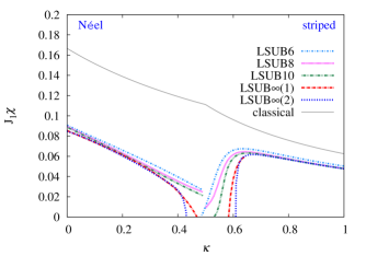
Figure 6: (Color online) CCM results for the zero-field magnetic susceptibility (in units of $J_{1}^{-1}$) versus the frustration parameter $\kappa\equiv J_{2}/J_{1}$, for the spin-$\frac{1}{2}$ $J_{1}$–$J_{2}$–$J_{3}$ model on the honeycomb lattice (with $J_{1}=1$, $J_{3}=J_{2}>0$). We show results based on the Néel and the striped AFM states as CCM model states. The LSUB$n$ results are shown with $n=\{6,8,10\}$, together with the extrapolated LSUB$\infty(1)$ and LSUB$\infty(2)$ results using Eqs. (28) and (29), respectively, with this data set. The classical results from Eqs. (12) and (13) are also shown for the value $s=\frac{1}{2}$.

For the striped collinear state used as the CCM model state, the number $N_{f}$ of fundamental configurations at the LSUB10 level is $N_{f}\approx 3.5\times 10^{5}$, and once again, just as for $\rho_{s}$ it is computationally infeasible to perform LSUB$n$ calculations for this phase with $n\geq 12$. By contrast, for the Néel state used as our CCM model state, $N_{f}\approx 6\times 10^{4}$ at the LSUB10 level and $N_{f}\approx 1.1\times 10^{6}$ at the LSUB12 level. In order to be consistent with our treatment of the two quasiclassical phases, we show the “raw” LSUB$n$ results in Fig. 6 with $n=\{6,8,10\}$ and corresponding LSUB$\infty$ extrapolations based on this data set. However, on the Néel side we have also performed an LSUB12 calculation for the unfrustrated limiting case $\kappa=0$. Once again, for comparison purposes, we also show in Fig. 6 the corresponding classical values obtained from Eqs. (12) and (13) by putting $J_{3}=J_{2}=\kappa J_{1}$ and $s=\frac{1}{2}$, viz., $\chi^{\rm N\acute{e}el}_{{\rm cl}}=1/[6J_{1}(1+\kappa)]$, and $\chi^{{\rm striped}}_{{\rm cl}}=1/[2J_{1}(1+7\kappa)]$.

Once again we see that quantum fluctuations act to reduce the value of $\chi$ considerably from its classical value in both quasiclassical AFM phases. Figure 6 also shows that the two extrapolation schemes of Eqs. (28) and (29) give results in very close agreement with one another on both sides of the phase diagram, except in very narrow regions close to the two QCPs at $\kappa=\kappa_{c_{1}}$ and $\kappa=\kappa_{c_{2}}$. Perhaps the most important feature of Fig. 6 is that, unlike in the classical case where $\chi_{{\rm cl}}$ takes the (nonzero) value $\frac{1}{9}$ at the phase transition point $\kappa_{{\rm cl}}=\frac{1}{2}$, in the quantum $s=\frac{1}{2}$ case $\chi$ now vanishes at the two QCPs, which is a very clear indication of a spin gap opening up at these points Mila (2000); Bernu and Lhuillier (2015).

We show in Fig. 6 extrapolated LSUB$\infty$ results based on the schemes of both Eqs. (28) and (29). The two sets of results shown are seen to be in excellent agreement with each other except in very narrow regimes close to the two QCPs at $\kappa_{c_{1}}$ and $\kappa_{c_{2}}$. Based on the scheme of Eq. (28), the two critical values obtained from extrapolating the LSUB$n$ values with $n=\{6,8,10\}$ are $\kappa_{c_{1}}\approx 0.469$ and $\kappa_{c_{2}}\approx 0.583$. The corresponding values from using scheme of Eq. (29) are $\kappa_{c_{1}}\approx 0.430$ and $\kappa_{c_{2}}\approx 0.609$. While both sets of results agree quite well with the corresponding results cited above of $\kappa_{c_{1}}\approx 0.448$ and $\kappa_{c_{2}}\approx 0.601$ from our earlier work on extrapolations for the magnetic order parameter of corresponding LSUB$n$ results with $n=\{6,8,10\}$, there is clearly more uncertainty in the critical values obtained from the zero-field magnetic susceptibility.

As an aside here, we remark that the shapes (e.g., the slopes) of the respective extrapolated (LSUB$\infty$) curves for $\rho_{s}$ and $\chi$ in Figs. 5 and 6 appear to vary significantly near where they vanish at the QCP $\kappa_{c_{1}}$, and also, but to a lesser extent, at the QCP $\kappa_{c_{2}}$. Clearly, in turn, this would imply different values for the critical indices for the two low-energy parameters at $\kappa_{c_{1}}$, in particular. However, we remain cautious about putting too much weight on such an interpretation, since it is precisely in the regions very close to the QCPs where the extrapolations become most demanding. While we are rather confident of the calculated values for $\kappa_{c_{1}}$ and $\kappa_{c_{2}}$ themselves, within errors we can estimate (and also see the further discussion below in Sec. V), the actual detailed shapes of the extrapolated curves (including, e.g., their slopes) at the QCPs is more open to doubt and the errors are more difficult to quantify. A close comparison of the raw LSUB$n$ families of curves and their respective LSUB$\infty$ extrapolations in Figs. 5 and 6 shows that the slopes of the raw and extrapolated curves very near to a supposedly continuous transition like that at $\kappa_{c_{1}}$ can differ appreciably. This difference is less marked at a first-order transition like that at $\kappa_{c_{2}}$, although still present to a lesser degree. For these reasons we are reluctant, with our present methodology and accuracy, to make any claims to be able to calculate, with any quantitative degree of accuracy, the critical indices for the vanishing of $\rho_{s}$ and $\chi$ at the two QCPs. Any such interpretation drawn from our results about the critical indices being different for $\rho_{s}$ and $\chi$ at $\kappa_{c_{1}}$ especially, should be regarded as suggestive at best, in our opinion.

It is also of interest to compare our results for $\chi$ for the limiting case $\kappa=0$ of a pure honeycomb HAF with NN interactions only. Our extrapolated LSUB$\infty$ results based on Eq. (28) are $\chi(\kappa=0)=0.0847(4)/J_{1}$, using LSUB$n$ data points $n=\{6,8,10,12\}$, where the quoted errors is purely that associated with the fit. Corresponding extrapolations based on LSUB$n$ results with $n=\{6,8,10\}$ and $n=\{8,10,12\}$ are, respectively, $\chi(\kappa=0)\approx 0.0845/J_{1}$ and $\chi(\kappa=0)\approx 0.0837/J_{1}$. Other estimates are $\chi(\kappa=0)\approx 0.0756(10)/J_{1}$ from a linked-cluster SE analysis Oitmaa et al. (1992); $\chi(\kappa=0)\approx 0.1667/J_{1}$ and $\chi(\kappa=0)\approx 0.0456/J_{1}$ from SWT at leading (classical) order and next-to-leading order [viz., with $O(1/s)$ corrections included], respectively Oitmaa et al. (1992); and $\chi(\kappa=0)=0.0666/J_{1}$ from SBMFT Mattsson et al. (1994). The most accurate estimates for this unfrustrated limit undoubtedly come from QMC calculations. For example, Löw Löw (2009) used a continuous Euclidean time QMC algorithm to find a value $\hat{\chi}(\kappa=0)=0.05188(8)/J_{1}$. Presumably, in the QMC calculations of the magnetic susceptibility the value $\hat{\chi}$ obtained is an average over all directions of the applied field, since the ground state is calculated for a finite system, i.e., with no breaking of the rotational symmetry. By contrast, in the CCM calculations we start with a symmetry-broken state and apply the field perpendicular to the axis of the order parameter, to obtain $\chi_{\perp}\,(\equiv\chi)$ directly. Thus, $\hat{\chi}=\frac{1}{3}(\chi_{\parallel}+2\chi_{\perp})$, where $\chi_{\parallel}\,(=0)$ is the parallel component of the magnetic susceptibility. Hence, we have $\chi=\frac{3}{2}\hat{\chi}$, and the QMC result of Löw is equivalent to $\chi(\kappa=0)=0.0778(1)/J_{1}$. Another QMC estimate, using a loop-cluster algorithm by Jiang Jiang (2012), can also be quoted. While Jiang does not quote a result for $\chi$ directly, he does provide the result $\hbar c(\kappa=0)=1.2905(8)J_{1}d$. This may be combined with his result for $\rho_{s}$ cited above to calculate $\chi=\rho_{s}/(\hbar c)^{2}$, yielding the value $\chi(\kappa=0)=0.0789(3)/J_{1}$. Clearly, our own best CCM estimate, $\chi(\kappa=0)=0.084(2)/J_{1}$, lies slightly higher than those two QMC estimates.

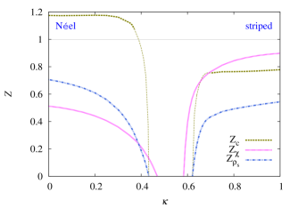
Figure 7: (Color online) CCM results for the three renormalization constants corresponding to the spin stiffness $\rho_{s}$, the zero-field magnetic susceptibility $\chi$, and the spin-wave velocity, $c$, of the spin-$\frac{1}{2}$ $J_{1}$–$J_{2}$–$J_{3}$ model on the honeycomb lattice with $J_{1}>0$, in the case $J_{3}=J_{2}=\kappa J_{1}$. Results for $Z_{c}$ are unreliable in the regions shown by thin lines, close to the critical points (and see text for details).

Table 1: The low-energy parameters for the spin-$\frac{1}{2}$ HAF on the honeycomb lattice with lattice spacing $d$ and with exchange interactions between NN pairs only, all with equal strength $J_{1}>0$. The classical values are compared with our CCM results, and those using the alternative techniques of linked-cluster SE Oitmaa et al. (1992) and two different QMC algorithms Löw (2009); Jiang (2012).

Parameter	Classical	CCM	SE	QMC	QMC
	value		(Ref. Oitmaa et al. (1992))	(Ref. Löw (2009))	(Ref. Jiang (2012))
$E/(NJ_{1})$	-0.375	-0.54466(2)	-0.5443(3)	-0.54455(20)
$M$	0.5	0.2714(10)	0.266(9)	0.2681(8)	0.26882(3)
$\rho_{s}/(J_{1}d^{2})$	0.1875	0.1324(5)			0.1315(3)
$J_{1}\chi$	0.1667	0.084(2)	0.0756(10)	0.07782(12)
$\hbar c/(J_{1}d)$	1.0607	1.255(15)			1.2905(8)

It is also convenient to express the low-energy parameters in terms of a multiplicative renormalization constant $Z$ with respect to the corresponding classical result. Thus, we define $Z_{\rho_{s}}$ and $Z_{\chi}$ as

$$Z_{\rho_{s}}\equiv\rho_{s}/\rho_{s;\,{\rm cl}}\,,\qquad Z_{\chi}\equiv\chi/\chi_{{\rm cl}}\,.$$ (30)

Since the spin-wave velocity is given by $\hbar c=\sqrt{\rho_{s}/\chi}$, its corresponding renormalization constant is

$$Z_{c}=\sqrt{Z_{\rho_{s}}/Z_{\chi}}\,.$$ (31)

Our extrapolated LSUB$\infty$ results for the three renormalization constants of Eqs. (30) and (31) are shown in Fig. 7, where we employ the LSUB$\infty(1)$ results for $\chi$ obtained from the extrapolation scheme of Eq. (28).

We should point out that the seeming vanishing of the Goldstone spin-wave velocity at both critical points $\kappa_{c_{1}}$ and $\kappa_{c_{2}}$, as shown in Fig. 7, is entirely an artefact of our calculational scheme. Thus, $Z_{c}$ has been calculated here indirectly via Eq. (31) using our (separately) extrapolated results for $\rho_{s}$ and $\chi$. In reality both of these parameters should go to zero at the same points (at least for $\chi$ at a transition at which a spin gap opens). However, as we have noted, our calculated results for $\rho_{s}$ and $\chi$ are completely independent of one another, and as a consequence the critical values at which both parameters vanish are not constrained to be the same. This is both a strength and a weakness of the methodology. The main advantage is that it provides an inbuilt error estimate for the accuracy of our calculated values of $\kappa_{c_{1}}$ and $\kappa_{c_{2}}$. However, it is also clearly a disadvantage when we wish to take ratios, as in Eq. (31), in regimes close to the QCPs. Thus, if $\rho_{s}$ and $\chi$ go to zero at slightly different values of $\kappa$, it is guaranteed that the spin-wave velocity calculated in terms of them will, quite artificially, approach either zero or infinity near the actual QCP. We have thus indicated in Fig. 7, by thinner portions of the curves for $Z_{c}$, those regions near the two QCPs where the results for $Z_{c}$ are correspondingly unreliable.

Finally, we collect in Table 1 our CCM results for the full set of low-energy parameters for the unfrustrated ($\kappa=0$) limiting case of a pure spin-$\frac{1}{2}$ HAF on the honeycomb lattice with NN interactions only (of strength $J_{1}>0$). We compare our results there with values obtained from a linked-cluster SE analysis Oitmaa et al. (1992), and two different QMC analyses Löw (2009); Jiang (2012), which are expected to be very accurate in this case, where the infamous minus-sign problem is absent. There is no reason to expect that the evident accuracy of our results in this limit will be any lower over the entire range of values of $\kappa$ accessible to us, by strong contrast with QMC techniques, which degrade significantly in the presence of frustration.

V SUMMARY AND CONCLUSIONS

In this paper we have continued our prior investigation Farnell et al. (2011) of the spin-$\frac{1}{2}$ $J_{1}$–$J_{2}$–$J_{3}$ HAF model on the honeycomb lattice, along the line $J_{3}=J_{2}=\kappa J_{1}$, with $J_{1}>0$, that includes the point of maximum classical frustration at $\kappa=\kappa_{{\rm cl}}=\frac{1}{2}$. Just as in our prior work we have used the CCM based on both the Néel and collinear striped AFM states as reference states, with respect to which we have included quantum fluctuations in the fully consistent LSUB$n$ truncation scheme. We have carried out calculations to high orders in the truncation index $n$ (typically with $n\leq 10$, but in some cases also with $n\leq 12$). The only approximation made has been to extrapolate in the truncation index $n$ to the exact ($n\rightarrow\infty$) LSUB$\infty$ limit.

We have now calculated a complete set of low-energy parameters ($E/N,M,\rho_{s},\chi$, and $c$) for the model, from which we obtain independent pieces of evidence that provide a clear and consistent description of its $T=0$ quantum phase diagram. In particular, we find compelling evidence that the single phase transition in the classical ($s\rightarrow\infty$) version of the model at $\kappa_{{\rm cl}}=\frac{1}{2}$ is split in the $s=\frac{1}{2}$ model into two quantum phase transitions at $\kappa_{c_{1}}$ and $\kappa_{c_{2}}$. In our prior work Farnell et al. (2011) these two QCPs were identified independently by the points at which both the magnetic order parameter $M$ and the inverse of the susceptibility coefficient against the formation of a state with PVBC order, $1/\chi_{p}$, vanish. To those estimates we now add two more, based on the points at which both $\rho_{s}$ and $\chi$ vanish. The collected results are displayed together in Table 2, in which the results for $M$ and $1/\chi_{p}$ are obtained Farnell et al. (2011) from LSUB$\infty$ extrapolation based on LSUB$n$ data points with $n=\{6,8,10,12\}$, while those for $\rho_{s}$ and $\chi$ are obtained from data points with $n=\{6,8,10\}$. All of our results are fully consistent with values $\kappa_{c_{1}}=0.45(2)$ and $\kappa_{c_{2}}=0.60(2)$.

Table 2: Values of the two quantum critical points $\kappa_{c_{1}}$ and $\kappa_{c_{2}}$ of the spin-$\frac{1}{2}$ $J_{1}$–$J_{2}$–$J_{3}$ HAF model on the honeycomb lattice, along the line $J_{3}=J_{2}=\kappa J_{1}$ with ($J_{1}>0$), as obtained from the vanishing points of the magnetic order parameter $M$, the spin stiffness $\rho_{s}$, the uniform magnetic susceptibility, and the inverse of the susceptibility coefficient of the system against the formation of PVBC order $1/\chi_{p}$, all evaluated by the extrapolation of CCM LSUB$n$ results.

Parameter ($\rightarrow 0$)	$\kappa_{c_{1}}$	$\kappa_{c_{2}}$
$M$ (see Ref. Farnell et al. (2011))	0.466	0.601
$\rho_{s}$ (this work)	0.433	0.621
$\chi$ (this work): LSUB$\infty(1)$ a	0.469	0.583
$\chi$ (this work): LSUB$\infty(2)$ b	0.430	0.609
$1/\chi_{p}$ (see Ref. Farnell et al. (2011))	0.473	0.586

^aUsing the extrapolation scheme of Eq. (28).
^bUsing the extrapolation scheme of Eq. (29).

Based on the shape of the curves for $M$ and $1/\chi_{p}$ as functions of $\kappa$ we suggested in our earlier work that the QCP at $\kappa_{c_{1}}$ between the state with Néel order (for $\kappa<\kappa_{c_{1}}$) and the paramagnetic intermediate state was of continuous type, while that at $\kappa_{c_{2}}$ between the state with collinear striped order (for $\kappa>\kappa_{c_{2}}$) and the intermediate state is of first-order type. The new evidence, based on $\rho_{s}$ and $\chi$, shown in Figs. 5 and 6 respectively, is completely consistent with this interpretation, as indeed is also the evidence based on the curves for the spin gap $\Delta$ shown in Figs. 4(a) and 4(b).

Since at a QCP the quantum fluctuations present in a system are sufficiently strong to make the system infinitely susceptibility to multiple forms of order, the vanishing of $1/\chi_{p}$ at $\kappa_{c_{1}}$ and $\kappa_{c_{2}}$ cannot be taken as strong evidence that PVBC order is present over the entire intermediate regime, $\kappa_{c_{1}}<\kappa<\kappa_{c_{2}}$. However, just as we could in this work find values of $\Delta$ into this regime in regions around both QCPs, so in our earlier work Farnell et al. (2011) could we calculate $\chi_{p}$ in similar regions. The shape of the curves for $1/\chi_{p}$ as a function of $\kappa$ was consistent with $1/\chi_{p}$ vanishing in those regions. It was on this evidence that we made the tentative conclusion that the entire region $\kappa_{c_{1}}<\kappa<\kappa_{c_{2}}$ contained a quantum phase with PVBC order.

The results of the present paper provide strong support for such an interpretation. Firstly, the vanishing of $\chi$ at $\kappa_{c_{1}}$ and $\kappa_{c_{2}}$ provides compelling evidence for a gapped state opening up at these points. Secondly, our results displayed in Fig. 4 provide positive and conclusive evidence of a gapped state over a considerable range of the intermediate regime, which is accessible using both quasiclassical AFM states as CCM model states. The values at which $\Delta$ becomes nonzero are also wholly consistent with the values for $\kappa_{c_{1}}$ and $\kappa_{c_{2}}$ cited above, as obtained from the GS low-energy parameters.

We note that Goldstone’s theorem implies that any state that breaks spin-rotational symmetry must have a vanishing gap. Thus, the non-vanishing of the triplet gap $\Delta$ in the intermediate phase completely rules out the possibility of any type of magnetic order being present in this regime, not only the Néel and striped forms considered explicitly here. Similarly, the fact that $\Delta\neq 0$ in the intermediate phase also precludes other more exotic forms of order that break SU(2) symmetry. Examples include spin-nematic states, which break SU(2) symmetry while preserving translational and time-reversal symmetries.

Finally, we note that it might also be interesting in future work to calculate the singlet excitation gap within the disordered regime, in order to compare it with the triplet gap calculated here. While the singlet gap can certainly also be calculated within the CCM framework, the calculations are more challenging, since the excited state now lies in the same sector as the ground state, viz., with $S^{z}_{T}=0$, where $S^{z}_{T}\equiv\sum^{N}_{i=1}s^{z}_{i}$. A possible motivation for doing so would be to compare with the corresponding results for the spin-$\frac{1}{2}$ $J_{1}$–$J_{2}$ HAF on the square lattice, the phase diagram for which is qualitatively similar to that for the spin-$\frac{1}{2}$ $J_{1}$–$J_{2}$–$J_{3}$ Heisenberg model on the honeycomb lattice, in the case $J_{3}=J_{2}$ considered here.

For example, a recent highly accurate density-matrix renormalization group (DMRG) simulation of the spin-$\frac{1}{2}$ $J_{1}$–$J_{2}$ Heisenberg model on the square lattice Jiang et al. (2012) found that the singlet gap remains consistently below the triplet gap over the intermediate disordered regime in this case. The authors took this finding as an indication of the formation of short-range singlets in the intermediate phase. In turn, this would be consistent with the intermediate phase being a spin liquid or one with only weak valence-bond crystalline (VBC) order. By contrast, a phase with stronger VBC order would be expected to have a triplon excitation as the lowest-energy excited state, since such a state corresponds to the breaking of only one singlet bond, compared to a singlet excitation that requires the breaking of two singlet bonds. If our conclusion for the present case of a spin-$\frac{1}{2}$ $J_{1}$–$J_{2}$–$J_{3}$ Heisenberg model on the honeycomb lattice (with $J_{3}=J_{2}$), that the intermediate phase has PVBC order, is correct, we would then expect the singlet excitation gap to lie higher than the triplet gap, by contrast with the above DMRG findings for the spin-$\frac{1}{2}$ HAF on the square lattice.

In conclusion, the present paper revisits a model to which the CCM had previously been applied, with the joint aims (and outcomes) to improve the conceptual framework and to yield new physics, particularly with regard to the nature of the intermediate phase. Thus, the calculation of a complete set of low-energy parameters for the model within a single, unified, and consistent theoretical CCM framework, has not only given more detailed information about each of the ordered magnetic phases and more accurate values for their boundaries with the intermediate (non-classical) disordered phase, but has also opened the possibility for a full (quantitative) $\chi$PT treatment of the model. Similarly, the CCM calculation of the triplet gap $\Delta$ has now definitively ruled out the intermediate phase from having any form of order that breaks SU(2) symmetry, including such exotic states as spin nematics.

References

- Mermin and Wagner (1966) N. D. Mermin and H. Wagner, Phys. Rev. Lett. 17, 1133 (1966).
- Oitmaa and Betts (1978) J. Oitmaa and D. D. Betts, Can. J. Phys 56, 897 (1978).
- Richter et al. (2004) J. Richter, J. Schulenburg, and A. Honecker, in Quantum Magnetism, Lecture Notes in Physics Vol. 645, edited by U. Schollwöck, J. Richter, D. J. J. Farnell, and R. F. Bishop (Springer-Verlag, Berlin, 2004) pp. 85–153.
- Weihong et al. (1991) Z. Weihong, J. Oitmaa, and C. J. Hamer, Phys. Rev. B 44, 11869 (1991).
- Mattsson et al. (1994) A. Mattsson, P. Fröjdh, and T. Einarsson, Phys. Rev. B 49, 3997 (1994).
- Oitmaa et al. (1992) J. Oitmaa, C. J. Hamer, and Z. Weihong, Phys. Rev. B 45, 9834 (1992).
- Reger et al. (1989) J. D. Reger, J. A. Riera, and A. P. Young, J. Phys.: Condens. Matter 1, 1855 (1989).
- Castro et al. (2006) E. V. Castro, N. M. R. Peres, K. S. D. Beach, and A. W. Sandvik, Phys. Rev. B 73, 054422 (2006).
- Jiang et al. (2008) F.-J. Jiang, F. Kämpfer, M. Nyfeler, and U.-J. Wiese, Phys. Rev. B 78, 214406 (2008).
- Löw (2009) U. Löw, Condensed Matter Physics 12, 497 (2009).
- Jiang (2012) F. Jiang, Eur. Phys. J. B 85, 402 (2012).
- Bishop and Rosenfeld (1998) R. F. Bishop and J. Rosenfeld, Int. J. Mod. Phys. B 12, 2371 (1998).
- Farnell et al. (2014) D. J. J. Farnell, O. Götze, J. Richter, R. F. Bishop, and P. H. Y. Li, Phys. Rev. B 89, 184407 (2014).
- Lieb et al. (1961) E. Lieb, T. Schultz, and D. Mattis, Ann. Phys. (N. Y.) 16, 407 (1961).
- Hastings (2004) M. B. Hastings, Phys. Rev. B 69, 104431 (2004).
- Tsirlin et al. (2010) A. A. Tsirlin, O. Janson, and H. Rosner, Phys. Rev. B 82, 144416 (2010).
- Miura et al. (2006) Y. Miura, R. Hirai, Y. Kobayashi, and M. Sato, J. Phys. Soc. Jpn. 75, 084707 (2006).
- Kataev et al. (2005) V. Kataev, A. Möller, U. Löw, W. Jung, N. Schittner, M. Kriener, and A. Freimuth, J. Magn. Magn. Mater. 290–291, 310 (2005).
- Okubo et al. (2011) S. Okubo, H. Wada, H. Ohta, T. Tomita, M. Fujisawa, T. Sakurai, E. Ohmichi, and H. Kikuchi, J. Phys. Soc. Jpn. 80, 023705 (2011).
- Möller et al. (2008) A. Möller, U. Löw, T. Taetz, M. Kriener, G. André, F. Damay, O. Heyer, M. Braden, and J. A. Mydosh, Phys. Rev. B 78, 024420 (2008).
- Yehia et al. (2010) M. Yehia, E. Vavilova, A. Möller, T. Taetz, U. Löw, R. Klingeler, V. Kataev, and B. Büchner, Phys. Rev. B 81, 060414(R) (2010).
- Rastelli et al. (1979) E. Rastelli, A. Tassi, and L. Reatto, Physica B & C 97, 1 (1979).
- Fouet et al. (2001) J. B. Fouet, P. Sindzingre, and C. Lhuillier, Eur. Phys. J. B 20, 241 (2001).
- Mulder et al. (2010) A. Mulder, R. Ganesh, L. Capriotti, and A. Paramekanti, Phys. Rev. B 81, 214419 (2010).
- Wang (2010) F. Wang, Phys. Rev. B 82, 024419 (2010).
- Cabra et al. (2011) D. C. Cabra, C. A. Lamas, and H. D. Rosales, Phys. Rev. B 83, 094506 (2011).
- Ganesh et al. (2011) R. Ganesh, D. N. Sheng, Y.-J. Kim, and A. Paramekanti, Phys. Rev. B 83, 144414 (2011).
- Clark et al. (2011) B. K. Clark, D. A. Abanin, and S. L. Sondhi, Phys. Rev. Lett. 107, 087204 (2011).
- Farnell et al. (2011) D. J. J. Farnell, R. F. Bishop, P. H. Y. Li, J. Richter, and C. E. Campbell, Phys. Rev. B 84, 012403 (2011).
- Reuther et al. (2011) J. Reuther, D. A. Abanin, and R. Thomale, Phys. Rev. B 84, 014417 (2011).
- Albuquerque et al. (2011) A. F. Albuquerque, D. Schwandt, B. Hetényi, S. Capponi, M. Mambrini, and A. M. Läuchli, Phys. Rev. B 84, 024406 (2011).
- Mosadeq et al. (2011) H. Mosadeq, F. Shahbazi, and S. A. Jafari, J. Phys.: Condens. Matter 23, 226006 (2011).
- Oitmaa and Singh (2011) J. Oitmaa and R. R. P. Singh, Phys. Rev. B 84, 094424 (2011).
- Mezzacapo and Boninsegni (2012) F. Mezzacapo and M. Boninsegni, Phys. Rev. B 85, 060402(R) (2012).
- Li et al. (2012a) P. H. Y. Li, R. F. Bishop, D. J. J. Farnell, J. Richter, and C. E. Campbell, Phys. Rev. B 85, 085115 (2012a).
- Bishop et al. (2012) R. F. Bishop, P. H. Y. Li, D. J. J. Farnell, and C. E. Campbell, J. Phys.: Condens. Matter 24, 236002 (2012).
- Bishop and Li (2012) R. F. Bishop and P. H. Y. Li, Phys. Rev. B 85, 155135 (2012).
- Li et al. (2012b) P. H. Y. Li, R. F. Bishop, D. J. J. Farnell, and C. E. Campbell, Phys. Rev. B 86, 144404 (2012b).
- Bishop et al. (2013) R. F. Bishop, P. H. Y. Li, and C. E. Campbell, J. Phys.: Condens. Matter 25, 306002 (2013).
- Ganesh et al. (2013) R. Ganesh, J. van den Brink, and S. Nishimoto, Phys. Rev. Lett. 110, 127203 (2013).
- Zhu et al. (2013) Z. Zhu, D. A. Huse, and S. R. White, Phys. Rev. Lett. 111, 257201 (2013).
- Zhang and Lamas (2013) H. Zhang and C. A. Lamas, Phys. Rev. B 87, 024415 (2013).
- Gong et al. (2013) S.-S. Gong, D. N. Sheng, O. I. Motrunich, and M. P. A. Fisher, Phys. Rev. B 88, 165138 (2013).
- Yu et al. (2014) X.-L. Yu, D.-Y. Liu, P. Li, and L.-J. Zou, Physica E 59, 41 (2014).
- Chakravarty et al. (1989) S. Chakravarty, B. I. Halperin, and D. R. Nelson, Phys. Rev. B 39, 2344 (1989).
- Neuberger and Ziman (1989) H. Neuberger and T. Ziman, Phys. Rev. B 39, 2608 (1989).
- Fisher (1989) D. S. Fisher, Phys. Rev. B 39, 11783 (1989).
- Hasenfratz and Leutwyler (1990) P. Hasenfratz and H. Leutwyler, Nucl. Phys. B343, 241 (1990).
- Hasenfratz and Niedermayer (1991) P. Hasenfratz and F. Niedermayer, Phys. Lett. B 268, 231 (1991).
- Hasenfratz and Niedermayer (1993) P. Hasenfratz and F. Niedermayer, Z. Phys. B 92, 91 (1993).
- Villain (1977) J. Villain, J. Phys. (France) 38, 385 (1977).
- Villain et al. (1980) J. Villain, R. Bidaux, J.-P. Carton, and R. Conte, J. Phys. (France) 41, 1263 (1980).
- Shender (1982) E. F. Shender, Zh. Eksp. Teor. Fiz. 83, 326 (1982), [Sov. Phys. JETP 56, 178 (1982)].
- Senthil et al. (2004a) T. Senthil, A. Vishwanath, L. Balents, S. Sachdev, and M. P. A. Fisher, Science 303, 1490 (2004a).
- Senthil et al. (2004b) T. Senthil, L. Balents, S. Sachdev, A. Vishwanath, and M. P. A. Fisher, Phys. Rev. B 70, 144407 (2004b).
- Bishop and Kümmel (1987) R. F. Bishop and H. G. Kümmel, Phys. Today 40(3), 52 (1987).
- Bartlett (1989) R. J. Bartlett, J. Phys. Chem. 93, 1697 (1989).
- Arponen and Bishop (1991) J. S. Arponen and R. F. Bishop, Ann. Phys. (N.Y.) 207, 171 (1991).
- Bishop (1991) R. F. Bishop, Theor. Chim. Acta 80, 95 (1991).
- Bishop (1998) R. F. Bishop, in Microscopic Quantum Many-Body Theories and Their Applications, Lecture Notes in Physics Vol. 510, edited by J. Navarro and A. Polls (Springer-Verlag, Berlin, 1998) p. 1.
- Roger and Hetherington (1990) M. Roger and J. H. Hetherington, Phys. Rev. B 41, 200 (1990).
- Bishop et al. (1992) R. F. Bishop, J. B. Parkinson, and Y. Xian, J. Phys.: Condens. Matter 4, 5783 (1992).
- Zeng et al. (1998) C. Zeng, D. J. J. Farnell, and R. F. Bishop, J. Stat. Phys. 90, 327 (1998).
- Farnell and Bishop (2004) D. J. J. Farnell and R. F. Bishop, in Quantum Magnetism, Lecture Notes in Physics Vol. 645, edited by U. Schollwöck, J. Richter, D. J. J. Farnell, and R. F. Bishop (Springer-Verlag, Berlin, 2004) p. 307.
- Krüger et al. (2006) S. E. Krüger, R. Darradi, J. Richter, and D. J. J. Farnell, Phys. Rev. B 73, 094404 (2006).
- Darradi et al. (2008) R. Darradi, O. Derzhko, R. Zinke, J. Schulenburg, S. E. Krüger, and J. Richter, Phys. Rev. B 78, 214415 (2008).
- Farnell et al. (2009) D. J. J. Farnell, R. Zinke, J. Schulenburg, and J. Richter, J. Phys.: Condens. Matter 21, 406002 (2009).
- Götze et al. (2011) O. Götze, D. J. J. Farnell, R. F. Bishop, P. H. Y. Li, and J. Richter, Phys. Rev. B 84, 224428 (2011).
- Bishop et al. (2014) R. F. Bishop, P. H. Y. Li, and C. E. Campbell, Phys. Rev. B 89, 214413 (2014).
- Li et al. (2015) P. H. Y. Li, R. F. Bishop, and C. E. Campbell, Phys. Rev. B 91, 014426 (2015).
- Richter et al. (2015) J. Richter, R. Zinke, and D. J. J. Farnell, Eur. Phys. J. B 88, 2 (2015).
- (72) We use the program package CCCM of D. J. J. Farnell and J. Schulenburg, see http://www-e.uni-magdeburg.de/jschulen/ccm/index.html.
- Krüger et al. (2000) S. E. Krüger, J. Richter, J. Schulenburg, D. J. J. Farnell, and R. F. Bishop, Phys. Rev. B 61, 14607 (2000).
- Gong et al. (2014) S.-S. Gong, W. Zhu, D. N. Sheng, O. I. Motrunich, and M. P. A. Fisher, Phys. Rev. Lett. 113, 027201 (2014).
- Mila (2000) F. Mila, Eur. J. Phys. 21, 499 (2000).
- Bernu and Lhuillier (2015) B. Bernu and C. Lhuillier, Phys. Rev. Lett. 114, 057201 (2015).
- Jiang et al. (2012) H.-C. Jiang, H. Yao, and L. Balents, Phys. Rev. B 86, 024424 (2012).