Achievable Rates for the Fading Half-Duplex Single Relay Selection Network Using Buffer-Aided Relaying

Abstract

In the half-duplex single relay selection network, comprised of a source, $M$ half-duplex relays, and a destination, only one relay is active at any given time, i.e., only one relay receives or transmits, and the other relays are inactive, i.e., they do not receive nor transmit. The capacity of this network, when all links are affected by independent slow time-continuous fading and additive white Gaussian noise (AWGN), is still unknown, and only achievable average rates have been reported in the literature so far. In this paper, we present new achievable average rates for this network which are larger than the best known average rates. These new average rates are achieved with a buffer-aided relaying protocol. Since the developed buffer-aided protocol introduces unbounded delay, we also devise a buffer-aided protocol which limits the delay at the expense of a decrease in rate. Moreover, we discuss the practical implementation of the proposed buffer-aided relaying protocols and show that they do not require more resources for channel state information acquisition than the existing relay selection protocols.

I Introduction

Cooperative communication has recently gained much attention due to its ability to increase the throughput and/or reliability of wireless networks. The basic idea behind cooperative communication is that each node can act as a relay and help the other nodes of the network to forward their information to their respective destination nodes. Because of the high complexity inherent to the investigation of general cooperative networks, and to get insight into the basic challenges and benefits of cooperative communication, researchers have mainly considered relatively simple cooperative networks. Although simple, these basic cooperative networks reveal the gains that can be accomplished by cooperation among network nodes. Moreover, because of their simplicity, these basic cooperative networks can be easily integrated into the current communication infrastructure. One basic network which has shown great potential in terms of utility and performance is the half-duplex (HD) single relay selection network proposed in [1]. In this network, only one relay is active at any given time, i.e., one relay receives or transmits, and the other relays are inactive, i.e., they do not receive nor transmit. Because of the large achievable performance gains, this network has recently attracted considerable interest, see [1]-[11] and references therein. Although well investigated, the capacity of this network is still unknown when all links are affected by independent slow time-continuous fading and additive white Gaussian noise (AWGN). So far, only achievable average rates have been reported in the literature, see [10, 11]. In fact, to the best of the authors’ knowledge, the achievable average rates in [10] and [11] are the largest average rates reported in the literature for this network. These rates are based on the relay selection protocol in [1], where, in each time slot, the relay with the strongest minimum source-to-relay and relay-to-destination channel is selected to forward the information from the source to the destination. In this paper, we will show that these rates can be surpassed. In particular, we develop a buffer-aided relaying protocol which achieves average rates which are significantly larger than the rates reported in [10] and [11]. Since the proposed buffer-aided protocol introduces unbounded delay, we also devise a second buffer-aided protocol which limits the average delay at the expense of a decrease in rate. Moreover, we show that the proposed buffer-aided relaying protocols do not require more resources for channel state information (CSI) acquisition than the existing relay selection protocols.

Buffer-aided HD relaying with adaptive switching between reception and transmission was proposed in [12] for a simple three-node relay network without source-destination link. Later, buffer-aided relaying was further analyzed in [13] and [14] for adaptive and fixed rate transmission, respectively. Buffer-aided relaying protocols were also proposed for two-way relaying in [15], [16], the multihop relay network in [17], two source and two destination pairs sharing a single relay in [18], secure communication for two-hop relaying and relay selection in [19] and [20], respectively, and amplify-and-forward relaying in [21]. For the considered relay selection network, relaying with buffers was investigated in [8] and [9]. However, the protocols in [8] and [9] are limited to the case when all nodes transmit with fixed rates and all source-to-relay and relay-to-destination links undergo independent and identically distributed (i.i.d.) fading. These protocols were developed for improving the outage probability performance of the network. In order to use the protocols in [8] and [9] as performance benchmarks, we modify them such that all nodes transmit with rates equal to their underlying channel capacities. However, the modified protocols are still only applicable to the case when all links are affected by i.i.d. fading and will cause data loss due to buffer overflow for independent non-identically distributed (i.n.d.) fading. We note however that this drawback is not caused by our modifications since the phenomenon of buffer overflow also occurs for the original protocols in [8] and [9] for fixed rate transmission when the links of the network are i.n.d.

This paper is organized as follows. In Section II, we introduce the system model. In Section  III, we present the proposed buffer-aided protocol for transmission without delay constraints. In Section IV, we discuss the implementation of the proposed protocol. In Section V, we propose a protocol for delay-limited transmission. In Section VI, we provide numerical examples comparing the achievable rates of the proposed protocols and the benchmark protocols. Finally, Section VII concludes the paper.

II System Model

In the following, we introduce the system model of the considered relay network. Furthermore, as benchmark scheme, we briefly review the conventional non-buffer-aided relay selection protocol in [1].

II-A System Model

The HD relay selection network consists of a source $S$, $M$ HD decode-and-forward relays $R_{k}$, $k=1,...,M$, and a destination $D$, as shown in Fig. 1. The source transmits its information to the destination only through the relays, i.e., because of high attenuation there is no direct link between the source and the destination, and therefore, all the information that the destination receives is first processed by the relays. We assume that the transmission is performed in $N$ time slots, where $N\to\infty$. The relays in the network are HD nodes, i.e., they cannot transmit and receive at the same time. Furthermore, in each time slot, only one relay is active, i.e., it receives or transmits, and the other relays are inactive, i.e., they do not receive nor transmit. Each relay is equipped with a buffer of unlimited size in which it stores the information that it receives from the source and from which it extracts the information that it transmits to the destination. We assume that all nodes transmit their codewords with constant power $P$ and that the noise at all receivers is independent AWGN with variance $\sigma_{n}^{2}$. We assume transmission with capacity achieving codes. Hence, the transmitted codewords are Gaussian distributed, comprised of $n\to\infty$ symbols, and span one time slot. Moreover, we assume that each source-to-relay and relay-to-destination channel is affected by independent slow time-continuous fading such that the fading remains constant during a single time slot and changes from one time slot to the next. We assume that the fading is an ergodic and stationary random process. Let $|h_{Sk}(i)|^{2}$ and $|h_{kD}(i)|^{2}$ denote the squared amplitudes of the complex channel gains of the source-to-$k$-th-relay and $k$-th-relay-to-destination channels in the $i$-th time slot, respectively, and let $\Omega_{Sk}=E\{|h_{Sk}(i)|^{2}\}$ and $\Omega_{kD}=E\{|h_{kD}(i)|^{2}\}$ denote their mean values, respectively, where $E\{\cdot\}$ denotes expectation. Then, the signal-to-noise ratios (SNRs) of the source-to-$k$-th-relay and $k$-th-relay-to-destination channels are given by

$$\gamma_{Sk}(i)=\frac{P}{\sigma_{n}^{2}}|h_{Sk}(i)|^{2}\;\textrm{ and }\;\gamma_{kD}(i)=\frac{P}{\sigma_{n}^{2}}|h_{kD}(i)|^{2},$$ (1)

respectively. Furthermore, we denote the average SNRs of the source-to-$k$-th-relay and $k$-th-relay-to-destination channels by $\bar{\gamma}_{Sk}=E\{\gamma_{Sk}(i)\}$ and $\bar{\gamma}_{kD}=E\{\gamma_{kD}(i)\}$, respectively. Using (1), the capacities of the source-to-$k$-th-relay and $k$-th-relay-to-destination channels in the $i$-th time slot, denoted by $C_{Sk}(i)$ and $C_{kD}(i)$, respectively, are given by

$$C_{Sk}(i) =\log_{2}\big{(}1+\gamma_{Sk}(i)\big{)}$$ (2)

$$C_{kD}(i) =\log_{2}\big{(}1+\gamma_{kD}(i)\big{)}.$$ (3)

[width=1]SysMod.eps

Figure 1: System model for buffer-aided relay selection.

II-B Conventional Relay Selection Protocol

For comparison purpose, we briefly review the conventional non-buffer-aided relay selection protocol [1] and its corresponding achievable average rate [10, 11].

The conventional relay selection protocol selects the relay $k$ with the maximum $\min\{C_{Sk}(i),C_{kD}(i)\}$ for forwarding the information from the source to the destination in the $i$-th time slot [1]. The channel coding scheme adopted for conventional relaying is as follows. In the first half of time slot $i$, the source sends a codeword with rate $\min\{C_{Sk}(i),C_{kD}(i)\}$ to the $k$-th relay. The $k$-th relay can successfully decode the received codeword since the rate of the codeword is smaller than or equal to $C_{Sk}(i)$. Then, in the second half of time slot $i$, the relay re-encodes the decoded information and sends it to the destination with rate $\min\{C_{Sk}(i),C_{kD}(i)\}$. The destination can successfully decode the received codeword since the rate of the codeword is smaller than or equal to $C_{kD}(i)$. Hence, the overall rate transmitted from source to destination during time slot $i$ is $\frac{1}{2}\min\{C_{Sk}(i),C_{kD}(i)\}$. Thereby, during $N\to\infty$ time slots, the average rate achieved with conventional relaying, denoted by $\bar{R}_{\rm conv}$, is obtained as [10, 11]

$$\bar{R}_{\rm conv}=\frac{1}{2}E\big{\{}\max_{k}\min\{C_{Sk}(i),C_{kD}(i)\}\big{\}}.$$ (4)

In the following, we present the proposed buffer-aided protocols for the considered relay selection network and the corresponding achievable rates.

III Buffer-Aided Relaying Protocol without Delay Constraint

In this section, we develop a buffer-aided relaying protocol without delay constraints which maximizes the achievable average rate for the considered network. To this end, we first introduce the instantaneous transmission rates at the nodes in each time slot, and then derive the corresponding achievable average rate. Next, we maximize the achievable average rate and derive analytical expressions for the maximum average rate.

III-A Instantaneous Transmission Rates

In the considered HD single relay selection network, in a given time slot, only one relay is selected to receive or transmit, i.e., to be active. Without loss of generality, assume that the $k$-th relay has been selected to be active in the $i$-th time slot. Then, if the active relay is selected to receive, the source maps $nR_{Sk}(i)$ bits of information to a Gaussian distributed codeword comprised of $n\to\infty$ symbols, where each symbol is generated independently according to a zero-mean complex circular-symmetric Gaussian distribution with variance $P$, and transmits this codeword to the selected relay. The rate of this codeword $R_{Sk}(i)$ is set as

$$R_{Sk}(i)=C_{Sk}(i),$$ (5)

where $C_{Sk}(i)$ is the capacity of the source-to-$k$-th-relay channel given in (2). As a result of (5), the active relay can successfully decode this codeword and stores the corresponding information in its buffer. Let $Q_{k}(i)$ denote the number of bits/symbol in the buffer of the $k$-th relay at the end of time slot $i$. Then, with this transmission, $Q_{k}(i)$ increases as

$$Q_{k}(i)=Q_{k}(i-1)+C_{Sk}(i).$$ (6)

On the other hand, if the active relay is selected to transmit, it extracts $nR_{kD}(i)$ bits of information from its buffer, maps it to a Gaussian distributed codeword comprised of $n\to\infty$ symbols, where each symbol is generated independently according to a zero-mean complex circular-symmetric Gaussian distribution with variance $P$, and transmits it to the destination. The rate of this codeword is $R_{kD}(i)$, which is set as

$$R_{kD}(i)=\min\{Q_{k}(i-1),C_{kD}(i)\},$$ (7)

where $C_{kD}(i)$ is the capacity of the $k$-th-relay-to-destination channel given in (2). The minimum in the expression for rate $R_{kD}(i)$ is a consequence of the fact that the relay cannot transmit more information than what it has stored in its buffer, i.e., more than $Q_{k}(i-1)$. The destination can successfully decode this codeword since $R_{kD}(i)\leq C_{kD}(i)$ holds, and stores the corresponding information. When the active relay transmits, $Q_{k}(i)$ decreases as

$$Q_{k}(i)=Q_{k}(i-1)-R_{kD}(i).$$ (8)

In the following, we obtain the average rates of buffer-aided single-relay selection.

III-B Average Transmission and Reception Rates

In order to derive the average rates of buffer-aided single-relay selection, we first have to model the reception and transmission of the $k$-th relay. To this end, we introduce two binary indicator variables $r_{k}^{\rm R}(i)\in\{0,1\}$ and $r_{k}^{\rm T}(i)\in\{0,1\}$, which indicate whether, in the $i$-th time slot, the $k$-th relay receives or transmits, respectively. More precisely, $r_{k}^{\rm R}(i)$ and $r_{k}^{\rm T}(i)$ are defined as

$$r_{k}^{\rm R}(i)\triangleq\left\{\begin{array}[]{cl}1&\textrm{if the }k\textrm{-th relay receives}\\ 0&\textrm{if the }k\textrm{-th relay does not receive},\end{array}\right.\;$$ (11)

$$r_{k}^{\rm T}(i)\triangleq\left\{\begin{array}[]{cl}1&\textrm{if the }k\textrm{-th relay transmits}\\ 0&\textrm{if the }k\textrm{-th relay does not transmit}.\end{array}\right.$$ (14)

Since exactly one relay is active in each time slot, $r_{k}^{\rm R}(i)$ and $r_{k}^{\rm T}(i)$ must satisfy

$$\sum_{k=1}^{M}[r_{k}^{\rm R}(i)+r_{k}^{\rm T}(i)]=1,\forall i.$$ (15)

Using $r_{k}^{\rm R}(i)$ and $r_{k}^{\rm T}(i)$, the average rates received at and transmitted by the $k$-th relay, denoted by $\bar{R}_{Sk}$ and $\bar{R}_{kD}$, respectively, can be expressed as

$$\bar{R}_{Sk} =\lim_{N\to\infty}\frac{1}{N}\sum_{i=1}^{N}r_{k}^{\rm R}(i)R_{Sk}(i)$$

$$=\lim_{N\to\infty}\frac{1}{N}\sum_{i=1}^{N}r_{k}^{\rm R}(i)C_{Sk}(i),$$ (16)

$$\bar{R}_{kD} =\lim_{N\to\infty}\frac{1}{N}\sum_{i=1}^{N}r_{k}^{\rm T}(i)R_{kD}(i)$$

$$=\lim_{N\to\infty}\frac{1}{N}\sum_{i=1}^{N}r_{k}^{\rm T}(i)\min\{Q_{k}(i-1),C_{kD}(i)\}.$$ (17)

Using $\bar{R}_{kD}$, $\forall k$, the average rate received at the destination, denoted by $\bar{R}_{SD}$, can be expressed as

$$\bar{R}_{SD} =\sum_{k=1}^{M}\bar{R}_{kD}$$

$$=\lim_{N\to\infty}\frac{1}{N}\sum_{i=1}^{N}\sum_{k=1}^{M}r_{k}^{\rm T}(i)\min\{Q_{k}(i-1),C_{kD}(i)\}.$$ (18)

In the following, our goal is to maximize $\bar{R}_{SD}$.

III-C Maximization of the Average Rate

In (16) and (17), the only variables with a degree of freedom are $r_{k}^{\rm R}(i)$ and $r_{k}^{\rm T}(i)$, $\forall i,k$. Any choice of these variables will provide an average rate. However, in order for an average rate to be achievable, i.e., for data loss not to occur, the buffers at all relays must remain stable. Moreover, among all the achievable average rates, there exists one rate which is the largest. In order to obtain the largest achievable average rate, we have to find the optimal values of $r_{k}^{\rm R}(i)$ and $r_{k}^{\rm T}(i)$, $\forall i,k$, which maximize the average rate in (III-B) when constraint (15) holds and when the buffers at all relays are stable. To this end, we introduce the following useful lemma.

Lemma 1

The achievable average rate is maximized when $r_{k}^{\rm R}(i)$ and $r_{k}^{\rm T}(i)$, $\forall i$, are chosen such that the following condition is satisfied for all $k=1,...,M$

$$\lim_{N\to\infty}\frac{1}{N}\sum_{i=1}^{N}r_{k}^{\rm R}(i)C_{Sk}(i)=\lim_{N\to\infty}\frac{1}{N}\sum_{i=1}^{N}r_{k}^{\rm T}(i)C_{kD}(i).$$ (19)

Moreover, when (19) holds for the $k$-th relay, (17) simplifies to

$$\bar{R}_{kD}=\lim_{N\to\infty}\frac{1}{N}\sum_{i=1}^{N}r_{k}^{\rm T}(i)C_{kD}(i),$$ (20)

and when (19) holds $\forall k$ relays, (III-B) simplifies to

$$\bar{R}_{SD}=\lim_{N\to\infty}\frac{1}{N}\sum_{i=1}^{N}\sum_{k=1}^{M}r_{k}^{\rm T}(i)C_{kD}(i).$$ (21)

Proof:

Please refer to Appendix -A. ∎

With Lemma 1, we have reduced the search space for the maximum achievable average rate to only those rates for which (19) holds $\forall k$. Moreover, we have obtained an expression for $\bar{R}_{SD}$ which is independent of $Q_{k}(i)$, $\forall i,k$. Now, in order to find the maximum achievable average rate, we devise a maximization problem for the average rate, $\bar{R}_{SD}$, under the constraints given in (19) and (15). This maximization problem, for $N\to\infty$, is given by

$$\begin{array}[]{ll}{\underset{r_{k}^{\rm R}(i),r_{k}^{\rm T}(i),\forall i,k}{\rm{Maximize:}}}&\frac{1}{N}\sum_{i=1}^{N}\sum_{k=1}^{M}r_{k}^{\rm T}(i)C_{kD}(i)\\ \vspace{1mm}{\rm{Subject\;\;to:}}&{\rm C1:}\,\frac{1}{N}\sum_{i=1}^{N}r_{k}^{\rm R}(i)C_{Sk}(i)\\ &\qquad=\frac{1}{N}\sum_{i=1}^{N}r_{k}^{\rm T}(i)C_{kD}(i),\;\forall k\\ \vspace{1mm}&{\rm C2:}\,r_{k}^{\rm R}(i)\in\{0,1\},\;\forall k,i\\ \vspace{1mm}&{\rm C3:}\,r_{k}^{\rm T}(i)\in\{0,1\},\;\forall k,i\\ \vspace{1mm}&{\rm C4:}\,\sum_{k=1}^{M}[r_{k}^{\rm R}(i)+r_{k}^{\rm T}(i)]=1,\;\forall i.\\ \end{array}$$ (28)

In (28), the restrictions in (19) and (15) are reflected in constraints C1 and C4, respectively. Fortunately, (28) can be solved analytically. The solution reveals how the values of $r_{k}^{\rm R}(i)$ and $r_{k}^{\rm T}(i)$ are to be chosen optimally in each time slot $i$ such that the maximum average rate of the buffer-aided protocol is achieved. Before providing the solution to (28), we first introduce some notations. Let $\mu_{k}$, $k=1,...,M$, denote constants which are independent of the time slot $i$ and the instantaneous CSI. The values of these constants depend on the fading statistics and will be determined later, cf. Lemma 2. Then, for a given time slot $i$, we multiply each $C_{Sk}(i)$ with $\mu_{k}$ and each $C_{kD}(i)$ with $(1-\mu_{k})$, and collect these products in set $\mathcal{A}(i)$. Hence, $\mathcal{A}(i)$ is given by

$$\mathcal{A}(i)=\big{\{}\mu_{1}C_{S1}(i),\mu_{2}C_{S2}(i),...,\mu_{M}C_{SM}(i),$$

$$(1-\mu_{1})C_{1D}(i),(1-\mu_{2})C_{2D}(i),...,(1-\mu_{M})C_{MD}(i)\big{\}}.$$ (29)

We are now ready to present the solution to (28) in the following theorem, which represents the proposed protocol for transmission without delay constraints.

Theorem 1

The optimal values of $r_{k}^{\rm T}(i)$ and $r_{k}^{\rm R}(i)$, $\forall k,i$ which maximize the achievable average rate of the proposed protocol are given by

$$\left\{\begin{array}[]{ll}\vspace{1mm}r_{k}^{\rm T}(i)=1&\textrm{if }\;(1-\mu_{k})C_{kD}(i)=\max\mathcal{A}(i)\\ \vspace{1mm}r_{k}^{\rm R}(i)=1&\textrm{if }\;\mu_{k}C_{Sk}(i)=\max\mathcal{A}(i)\\ r_{k}^{\rm T}(i)=r_{k}^{\rm R}(i)=0&\textrm{otherwise},\end{array}\right.$$ (33)

where the $\mu_{k}$, $\forall k$, are chosen such that constraint C1 in (28) is satisfied $\forall k$. The maximum achievable average rate of the proposed protocol is given by (21) when $r_{k}^{\rm R}(i)$ and $r_{k}^{\rm T}(i)$ are set as in (33), $\forall i,k$.

Proof:

Please see Appendix -B. ∎

Remark 1

Theorem 1 reveals that the optimal values of $r_{k}^{\rm R}(i)$ and $r_{k}^{\rm T}(i)$ depend only on the instantaneous CSI of the $i$-th time slot, and are independent of the instantaneous CSIs of past and future time slots.

III-D Analytical Characterization of the Maximum Achievable Rate

By inserting (33) into (III-B), we obtain the maximum achievable rate of the proposed protocol as an average over $N\to\infty$ time slots, which may not be convenient from an analytical point of view. Furthermore, Theorem 1 does not provide an expression for obtaining constants $\mu_{k}$, $\forall k$. In order to obtain useful analytical expressions for the maximum achievable average rate and constants $\mu_{k}$, $\forall k$, we exploit the assumed ergodicity and stationarity of the fading, and write (19) (i.e., constraint C1 in (28)) and (21) equivalently as

$$\left\{\begin{array}[]{lll}E\{\log_{2}(1+\Gamma_{S1}(i))\}&=&E\{\log_{2}(1+\Gamma_{1D}(i))\}\\ E\{\log_{2}(1+\Gamma_{S2}(i))\}&=&E\{\log_{2}(1+\Gamma_{2D}(i))\}\\ &\vdots&\\ E\{\log_{2}(1+\Gamma_{SM}(i))\}&=&E\{\log_{2}(1+\Gamma_{MD}(i))\}\end{array}\right.$$ (38)

and

$$\bar{R}_{SD} = \sum_{k=1}^{M}E\{\log_{2}(1+\Gamma_{kD}(i))\},$$ (39)

respectively, where $\Gamma_{Sk}(i)=r^{\rm R}_{k}(i)\gamma_{Sk}(i)$ and $\Gamma_{kD}(i)=r^{\rm T}_{k}(i)\gamma_{kD}(i)$, with $r_{k}^{\rm R}(i)$ and $r_{k}^{\rm T}(i)$ as in (33). In the following two lemmas, we provide simplified expressions for the maximum average rate $\bar{R}_{SD}$ and constants $\mu_{k}$, $\forall k$. Thereby, we drop index $i$ since, due to the stationarity and ergodicity of the fading, the statistics of $\Gamma_{Sk}(i)$ and $\Gamma_{kD}(i)$ are independent of $i$.

Lemma 2

The optimal values of $\mu_{k}$, $k=1,...,M$, denoted by $\mu_{k}^{*}$, which maximize $\bar{R}_{SD}$, can be obtained by solving the following system of $M$ equations

$$\left\{\begin{array}[]{lll}\int_{0}^{\infty}\log_{2}(1+x)f_{\Gamma_{S1}}(x)dx=\int_{0}^{\infty}\log_{2}(1+x)f_{\Gamma_{1D}}(x)dx\\ \int_{0}^{\infty}\log_{2}(1+x)f_{\Gamma_{S2}}(x)dx=\int_{0}^{\infty}\log_{2}(1+x)f_{\Gamma_{2D}}(x)dx\\ \hskip 113.81102pt\vdots\\ \int_{0}^{\infty}\log_{2}(1+x)f_{\Gamma_{SM}}(x)dx=\int_{0}^{\infty}\log_{2}(1+x)f_{\Gamma_{MD}}(x)dx,\end{array}\right.$$ (44)

where, for $x>0$,

$$f_{\Gamma_{Sk}}(x)=f_{\gamma_{Sk}}(x)F_{\gamma_{kD}}\left((1+x)^{\frac{\mu_{k}}{1-\mu_{k}}}-1\right)$$

$$\qquad\times\prod_{\underset{j\neq k}{j=1}}^{M}F_{\gamma_{Sj}}\left((1+x)^{\frac{\mu_{k}}{\mu_{j}}}-1\right)F_{\gamma_{jD}}\left((1+x)^{\frac{\mu_{k}}{1-\mu_{j}}}-1\right),$$ (45)

$$f_{\Gamma_{kD}}(x)=f_{\gamma_{kD}}(x)F_{\gamma_{Sk}}\left((1+x)^{\frac{1-\mu_{k}}{\mu_{k}}}-1\right)$$

$$\times\prod_{\underset{j\neq k}{j=1}}^{M}F_{\gamma_{Sj}}\left((1+x)^{\frac{1-\mu_{k}}{\mu_{j}}}-1\right)F_{\gamma_{jD}}\left((1+x)^{\frac{1-\mu_{k}}{1-\mu_{j}}}-1\right).$$ (46)

Here, $f_{\gamma_{\alpha}}(x)$ and $F_{\gamma_{\alpha}}(x)$ denote the probability density function (PDF) and cumulative distribution function (CDF) of $\gamma_{\alpha}$, $\alpha\in\{Sk,kD\}$, respectively. Furthermore, if the fading on all source-to-relay and relay-to-destination links is i.i.d., the solution to (44) is $\mu_{k}^{*}=1/2$, $\forall k$.

Proof:

Please refer to Appendix -C. ∎

Remark 2

For i.i.d. links, since $\mu_{k}^{*}=1/2$, $\forall k$, the proposed protocol, given by (33), always selects the link with the largest instantaneous channel gain among all $2M$ available links for transmission. Hence, for i.i.d. links this protocol becomes identical to the protocol proposed in [8]. However, for i.n.d. links, the protocol in [8] will cause data loss due to buffer overflow. In particular, applying the protocols in [8] and [9], the buffers at relays with $\Omega_{Sk}>\Omega_{kD}$ suffer from overflow and receive more information than they can transmit. Hence, a fraction of the source’s data is trapped inside the relay buffers and does not reach the destination, i.e., data loss occurs. On the other hand, our proposed protocol is applicable for all fading statistics.

Lemma 3

The maximum achievable average rate of the protocol in Theorem 1 is given by

$$\bar{R}_{SD}=\sum_{k=1}^{M}\int_{0}^{\infty}\log_{2}(1+x)f_{\Gamma_{kD}}^{*}(x)dx,$$ (47)

where $f_{\Gamma_{kD}}^{*}(x)$ is obtained by inserting $\mu_{k}=\mu_{k}^{*}$ found using Lemma 2 into $f_{\Gamma_{kD}}(x)$ given by (46). For i.i.d. fading on all links, i.e., when $f_{\gamma_{Sk}}(x)=f_{\gamma_{kD}}(x)=f_{\gamma}(x)$, $\forall k$, and $F_{\gamma_{Sk}}(x)=F_{\gamma_{kD}}(x)=F_{\gamma}(x)$, $\forall k$, (47) simplifies to

$$\bar{R}_{SD}=M\int_{0}^{\infty}\log_{2}(1+x)f_{\gamma}(x)\left(F_{\gamma}(x)\right)^{2M-1}dx.$$ (48)

Proof:

Let us insert the optimal $\mu_{k}^{*}$, $\forall k$, found from Lemma 2, into $f_{\Gamma_{kD}}(x)$ given in (46) and denote it by $f_{\Gamma_{kD}}^{*}(x)$. Eq. (47) is obtained by inserting $f_{\Gamma_{kD}}^{*}(x)$ into (39), whereas (48) is obtained by inserting $\mu^{*}=1/2$ into (47) and simplifying the resulting expression. ∎

To get more insight, in the following we investigate the case of i.i.d. Rayleigh fading.

III-E Special Case: I.i.d. Rayleigh Fading

In the following, we simplify the expression for the maximum average rate in (48) for i.i.d. Rayleigh fading.

The expression $f_{\gamma_{\max}}(x)=2Mf_{\gamma}(x)\left(F_{\gamma}(x)\right)^{2M-1}$ in (48) can be interpreted as the distribution of the largest random variable (RV) among $2M$ i.i.d. RVs with distributions $f_{\gamma_{Sk}}(x)=f_{\gamma_{kD}}(x)=f_{\gamma}(x)$, $\forall k$, see [23]. For i.i.d. Rayleigh fading, i.e., when $f_{\gamma_{Sk}}(x)=f_{\gamma_{kD}}(x)=e^{-x/\bar{\gamma}}/\bar{\gamma}$, $\forall k$, where $\bar{\gamma}$ is the average SNR of all source-to-relay and relay-to-destination links, $f_{\gamma_{\max}}(x)$ is given as [23]

$$f_{\gamma_{\max}}(x)=2M\sum_{k=0}^{2M-1}(-1)^{k}{2M-1\choose k}\frac{1}{\bar{\gamma}}\exp\left(-\frac{x}{\bar{\gamma}}(k+1)\right).$$ (49)

Inserting (49) into (48) and integrating, we obtain the average rate as

$$\bar{R}_{SD} =M\sum_{k=0}^{2M-1}{2M-1\choose k}\frac{(-1)^{k}}{(1+k)\ln(2)}\exp\left(\frac{1+k}{\bar{\gamma}}\right)$$

$$\times E_{1}\left(\frac{1+k}{\bar{\gamma}}\right),$$ (50)

where $E_{1}(\cdot)$ is the first order exponential integral function defined as $E_{1}(x)=\int_{1}^{\infty}e^{-xt}/(t)dt$. On the other hand, for the same case, i.e., for i.i.d. Rayleigh fading on all links, the achievable rate for conventional relay selection given in (4) can be written equivalently as [24, Eq. (26)]

$$\bar{R}_{\rm conv} =\frac{M}{2}\sum_{k=0}^{M-1}{M-1\choose k}\frac{(-1)^{k}}{(1+k)\ln(2)}\exp\left(\frac{2(1+k)}{\bar{\gamma}}\right)$$

$$\times E_{1}\left(\frac{2(1+k)}{\bar{\gamma}}\right).$$ (51)

In order to gain further insight, expressions (50) and (III-E) can be further simplified for low and high SNRs using the following first order Taylor approximations

$$\exp(c/\bar{\gamma})E_{1}\left(c/\bar{\gamma}\right)=\frac{c}{\bar{\gamma}},\textrm{ as }\bar{\gamma}\to 0,$$ (52)

$$\exp(c/\bar{\gamma})E_{1}\left(c/\bar{\gamma}\right)=-K_{EM}-\ln(c)+\ln(\bar{\gamma}),\textrm{ as }\bar{\gamma}\to\infty,$$ (53)

where $K_{EM}$ is the Euler-Mascheroni constant and its value is $K_{EM}\approx 0.577$.

III-E1 Low SNR

Using (52), the rates in (50) and (III-E) can be approximated as

$$\bar{R}_{SD}\to\frac{\bar{\gamma}}{2\ln(2)}\sum_{k=1}^{2M}\frac{1}{k},\textrm{ as }\bar{\gamma}\to 0$$ (54)

$$\bar{R}_{\rm conv}\to\frac{\bar{\gamma}}{4\ln(2)}\sum_{k=1}^{M}\frac{1}{k},\textrm{ as }\bar{\gamma}\to 0.$$ (55)

Dividing (54) by (55), we obtain the following ratio

$$\frac{\bar{R}_{SD}}{\bar{R}_{\rm conv}}=2\frac{\sum_{k=1}^{2M}\frac{1}{k}}{\sum_{k=1}^{M}\frac{1}{k}}.$$ (56)

For $M=1$ and $M\to\infty$, the ratio in (56) is equal to $3$ and $2$, respectively, which constitute the upper and lower bounds of (56) for $1\leq M\leq\infty$. Hence, for low SNRs, the average rate of the proposed buffer-aided relay selection protocol is $2$ to $3$ times higher than the rate of conventional relay selection.

III-E2 High SNR

On the other hand, using (53), the rates in (50) and (III-E) can be approximated as

$$\bar{R}_{SD}\to\frac{\bar{\gamma}-K_{EM}}{2\ln(2)}$$

$$-M\sum_{k=0}^{2M-1}{2M-1\choose k}\frac{(-1)^{k}\log_{2}(1+k)}{(1+k)},\textrm{ as }\bar{\gamma}\to\infty,$$ (57)

$$\bar{R}_{\rm conv}\to\frac{\bar{\gamma}-K_{EM}}{2\ln(2)}$$

$$\quad-\frac{M}{2}\sum_{k=0}^{M-1}{M-1\choose k}\frac{(-1)^{k}\log_{2}(1+k)}{(1+k)}-\frac{1}{2},\textrm{ as }\bar{\gamma}\to\infty.$$ (58)

Subtracting (58) from (57), we obtain

$$\bar{R}_{SD}-\bar{R}_{\rm conv} =\frac{1}{2}+\frac{M}{2}\sum_{k=0}^{M-1}{M-1\choose k}\frac{(-1)^{k}\log_{2}(1+k)}{(1+k)}$$

$$-M\sum_{k=0}^{2M-1}{2M-1\choose k}\frac{(-1)^{k}\log_{2}(1+k)}{(1+k)}.$$ (59)

For $M=1$ and $M\to\infty$, the expression in (59) evaluates to $1$ and $1/2$, respectively, which constitute the upper and lower bounds of (59) for $1\leq M\leq\infty$. Hence, for high SNRs, the average rate of the proposed buffer-aided relay selection protocol is between $1$ and $1/2$ bits/symb larger than the rate of conventional relay selection.

In the following, we discuss the implementation of the proposed buffer-aided HD relay selection protocol.

IV Implementation of the Proposed Buffer-Aided Protocol

In this section, we discuss the implementation of the protocol proposed in Theorem 1. The proposed protocol can be implemented in a centralized or in a distributed manner. A centralized implementation assumes a central node which selects the active relay in each time slot and decides whether it should receive or transmit. On the other hand, in the distributed implementation, there is no central node and the relays themselves negotiate which relay should be active in each time slot. In the following, we discuss both implementations.

IV-A Centralized Implementation

For the centralized implementation, we assume that the destination is the central node. Hence, in each time slot, the destination has to obtain the CSI of all links. To this end, at the beginning of each time slot, the source transmits pilot symbols from which all relays acquire their respective source-to-relay CSIs. Then, each relay broadcasts orthogonal pilots, from which the source and destination learn all source-to-relay and relay-to-destination CSIs, respectively. Next, each relay feedsback the CSI of its respective source-to-relay channel to the destination. With the acquired CSI, the destination computes $C_{Sk}(i)$ and $C_{kD}(i)$, $\forall k$. In order to select the active relay according to the protocol in Theorem 1, the destination has to construct set $\mathcal{A}(i)$, given by (III-C). This requires the computation of the constants $\mu_{k}$, $\forall k$. These constants can be computed using Lemma 2, but this requires knowledge of the PDFs of the fading gains of all links before the start of transmission. Such a priori knowledge may not be available in practice. In this case, the destination has to estimate $\mu_{k}$, $\forall k$, in real-time using only the CSI knowledge until time slot $i$. Since $\mu_{k}$, $\forall k$, are actually Lagrange multipliers obtained by solving the linear optimization problem in (78), an accurate estimate of $\mu_{k}$, $\forall k$, can be obtained using the gradient descent method [25]. In particular, using $C_{Sk}(i)$ and $C_{kD}(i)$, the destination recursively computes an estimate of $\mu_{k}$, denoted by $\mu_{k}^{e}(i)$, as

$$\mu_{k}^{e}(i)=\mu_{k}^{e}(i-1)+\delta_{k}(i)(\bar{R}_{kD}^{e}(i-1)-\bar{R}_{Sk}^{e}(i-1)),$$ (60)

where $\bar{R}_{Sk}^{e}(i-1)$ and $\bar{R}_{kD}^{e}(i-1)$ are real-time estimates of $\bar{R}_{Sk}$ and $\bar{R}_{kD}$, respectively, computed for $i\geq 2$ as

$$\bar{R}_{Sk}^{e}(i-1) =\frac{i-2}{i-1}\bar{R}_{Sk}^{e}(i-2)+\frac{r_{k}^{\rm R}(i-1)}{i-1}C_{Sk}(i-1),$$ (61)

$$\bar{R}_{kD}^{e}(i-1) =\frac{i-2}{i-1}\bar{R}_{kD}^{e}(i-2)+\frac{r_{k}^{\rm T}(i-1)}{i-1}C_{kD}(i-1),$$ (62)

where $R_{Sk}^{e}(0)$ and $R_{kD}^{e}(0)$ are set to zero $\forall k$. In (60), $\delta_{k}(i)$ is an adaptive step size which controls the speed of convergence of $\mu_{k}^{e}(i)$ to $\mu_{k}$. In particular, the step size $\delta_{k}(i)$ is some properly chosen monotonically decaying function of $i$ with $\delta_{k}(1)<1$, see [25] for more details.

Once the destination has $C_{Sk}(i)$, $C_{kD}(i)$, and $\mu_{k}^{e}(i)$, $\forall k$, it constructs the set $\mathcal{A}(i)$, and selects the active relay according to Theorem 1. The destination also has to keep track of the queue length in the buffers at each relay in each time slot. To this end, using $C_{Sk}(i)$, $C_{kD}(i)$, $r_{k}^{\rm R}(i)$, and $r_{k}^{\rm T}(i)$, $\forall k$, the destination computes the queue length in the buffers at each relay using the following formula

$$Q_{k}(i) =Q_{k}(i-1)+r_{k}^{\rm R}(i)C_{Sk}(i)$$

$$-r_{k}^{\rm T}(i)\min\{Q_{k}(i-1),C_{kD}(i)\}.$$ (63)

Then, the destination broadcasts a control message to the relays which contains information regarding which relay is selected and whether it will receive or transmit. If the selected relay is scheduled to transmit, it extracts information bits from its buffer, maps them to a codeword, and transmits the codeword to the destination with rate $R_{kD}(i)=\min\{Q_{k}(i-1),C_{kD}(i)\}$. Otherwise, if the selected relay is scheduled to receive, it sends a control message to the source which informs the source which relay is selected. Then, the source transmits the information codeword intended for the selected relay with rate $R_{Sk}(i)=C_{Sk}(i)$.

The destination may receive the information bits in an order which is different from that in which they were transmitted by the source. However, using the acquired CSI, the destination can keep track of the amount of information received and transmitted by each relay in each time slot. This information is sufficient for the destination to perform successful reordering of the received information bits.

IV-B Distributed Implementation

We now outline the distributed implementation of the proposed protocol using timers, similar to the scheme in [1].

At the beginning of time slot $i$, source and destination transmit pilots in successive pilot time slots. This enables the relays to acquire the CSI of their respective source-to-relay and relay-to-destination channels, respectively. Using the acquired CSI, the $k$-th relay computes $C_{Sk}(i)$ and $C_{kD}(i)$. Next, using $C_{Sk}(i)$ and $C_{kD}(i)$, the $k$-th relay computes the estimate of $\mu_{k}$, $\mu_{k}^{e}(i)$, using (60), (61), and (62). Using $C_{Sk}(i)$, $C_{kD}(i)$, and $\mu_{k}^{e}(i)$, the $k$-th relay turns on a timer proportional to $1/\max\{\mu_{k}^{e}(i)C_{Sk}(i),(1-\mu_{k}^{e}(i))C_{kD}(i)\}$. This procedure is performed by all $M$ relays. If

$$\max\{\mu_{k}^{e}(i)C_{Sk}(i),(1-\mu_{k}^{e}(i))C_{kD}(i)\}=\mu_{k}^{e}(i)C_{Sk}(i)$$

and

$$\max\{\mu_{k}^{e}(i)C_{Sk}(i),(1-\mu_{k}^{e}(i))C_{kD}(i)\}=(1-\mu_{k}^{e}(i))C_{kD}(i),$$

the $k$-th relay knows that if it is selected, then it will receive and transmit, respectively. The relay whose timer expires first, broadcasts a packet containing pilot symbols and a control message with information about which relay is selected and whether the selected relay receives or transmits. From the packet broadcasted by the selected relay, both source and destination learn the channels from the selected relay to the source and destination, respectively. They also learn which relay is selected and whether it is scheduled to receive or transmit. If the selected relay is scheduled to transmit, then it extracts bits from its buffer, maps them to a codeword and transmits the codeword to the destination with rate $R_{kD}(i)=\min\{Q_{k}(i-1),C_{kD}(i)\}$. Otherwise, if the relay is scheduled to receive, then the source transmits to the selected relay a codeword with rate $C_{Sk}(i)$.

Again, the destination may receive the information bits in an order which is different from that in which they were transmitted by the source. Therefore, in order for the destination to reorder the received information bits, it should keep track of the amount of information received and transmitted by each relay in each time slot. If the selected relay transmits, by successful decoding the destination learns the amount of information received. However, when the selected relay is scheduled to receive, the relay should feedback the amount of information that it received to the destination. Using this information, the destination can perform successful reordering of the received information bits.

Remark 3

We note that distributed relay selection protocols based on timers may suffer from long waiting times before the first timer expires. Moreover, collisions are possible when two or more relay nodes declare that they are the selected node at approximately the same time. However, by choosing the timers suitably, as proposed in [26], these negative effects can be minimized.

IV-C Comparison of the Overhead of the Conventional and the Proposed Protocols

The conventional relay selection protocol reviewed in Section II-B can also be implemented in a centralized or a distributed manner. In the following, we discuss the overheads entailed by both implementations.

For the centralized implementation, the destination controls the relay selection. To this end, the destination has to acquire the CSI of all links in the network. Therefore, for centralized implementation, in each time slot, $2M+2$ pilot symbol transmissions are required for CSI acquisition, one control packet transmission by the destination is needed to inform the relays which relay is selected, and another control packet transmission is required for the selected relay to inform the source which relay is selected. Moreover, the source has to acquire knowledge of $\min\{C_{Sk}(i),C_{kD}(i)\}$ in order to select the rate of transmission. Hence, if $\min\{C_{Sk}(i),C_{kD}(i)\}=C_{kD}(i)$, the selected relay has to feedback the CSI of the selected-relay-to-destination link to the source. As a result, in total $2M+4$ or $2M+5$ pilot symbol, feedback, and control packet transmissions are needed in each time slot. On the other hand, for the centralized implementation of the proposed buffer-aided relaying protocol, also $2M+4$ or $2M+5$ pilot symbol, feedback, and control packet transmissions are required. Hence, both the conventional and the proposed buffer-aided relaying protocols have identical overheads when implemented centrally.

For conventional relay selection with distributed implementation, each relay has to acquire the CSI of its source-to-relay and relay-to-destination links. To this end, two pilot transmissions, one from the source and the other from the destination, are needed. Moreover, one packet with pilots and a control message from the selected relay are needed to inform source and destination which relay is selected, and to allow source and destination to learn the CSI of the source-to-selected-relay and selected-relay-to-destination links, respectively. Furthermore, assuming relay $k$ is the selected relay in time slot $i$, in order for the source to adapt its transmission rate to $\min\{C_{Sk}(i),C_{kD}(i)\}$ and the destination to know which codebook to use for decoding in time slot $i$, both source and relay have to know $\min\{C_{Sk}(i),C_{kD}(i)\}$. Acquiring this CSI knowladge requires feedback of the source-to-relay or the relay-to-destination channel from the relay to the destination or the source, respectively. Hence, the distributed implementation of conventional relay selection requires $4$ pilot symbol, feedback, and control packet transmissions. On the other hand, the distributed implementation of the proposed buffer-aided relaying protocol has the same overhead as conventional relay selection since it also requires $4$ pilot symbol, feedback, and control packet transmissions.

As can be seen from the above discussion, the proposed buffer-aided protocol does not require more signaling overhead than the conventional relay selection protocol. We note, however, that the proposed protocol requires the computation of $\mu_{k}^{e}(i)$ and $Q_{k}(i)$, $\forall k$, which are not required for the conventional protocols. On the other hand, the computational complexity of obtaining $\mu_{k}^{e}(i)$ and $Q_{k}(i)$ using (60)-(62) and (IV-A), respectively, is not high since these equations require only one or two additions and one to three multiplications.

V Buffer-Aided Relaying Protocol with a Delay Constraint

The protocol in Theorem 1, with the $\mu_{k}^{*}$, $\forall k$, obtained from Lemma 2, gives the maximum average achievable rate, but introduces unbounded delay. To bound the delay, in the following, we propose a buffer-aided relaying protocol for delay limited transmission. Before presenting the protocol, we first determine the average delay for the considered network.

V-A Average Delay

The average delay for the considered network, denoted by $\bar{T}$, is specified in the following lemma.

Lemma 4

The average delay for the considered network is given by

$$\bar{T}=\frac{\sum_{k=1}^{M}\bar{Q}_{k}}{\sum_{k=1}^{M}\bar{R}_{Sk}},$$ (64)

where $\bar{R}_{Sk}$ is the average rate received at the $k$-th relay and given by (16). Furthermore, $\bar{Q}_{k}$ is the average queue size in the buffer of the $k$-th relay, which is found as

$$\bar{Q}_{k}=\lim_{N\to\infty}\frac{1}{N}\sum_{i=1}^{N}Q_{k}(i).$$ (65)

Proof:

Please refer to Appendix -D. ∎

The queue size at time slot $i$ can be obtained using (IV-A). Due to the recursiveness of the expression in (IV-A), it is difficult, if not impossible, to obtain an analytical expression for the average queue size $\bar{Q}_{k}$ for a general buffer-aided relay selection protocol. Hence, in contrast to the case without delay constraint, for the delay limited case, it is very difficult to formulate an optimization problem for maximization of the average rate subject to some average delay constraint. As a result, in the following, we develop a simple heuristic protocol for delay limited transmission. The proposed protocol is a distributed protocol in the sense that the relays themselves negotiate which relay should receive or transmit in each time slot such that the average delay constraint is satisfied. We note that the proposed protocol does not need any knowledge of the statistics of the channels.

V-B Distributed Buffer-Aided Protocol

Before presenting the proposed heuristic protocol for delay limited transmission, we first explain the intuition behind the protocol.

V-B1 Intuition Behind the Protocol

Assume that we have a buffer-aided protocol which, when implemented in the considered network, enforces the following relation

$$\frac{\bar{Q}_{k}}{\bar{R}_{Sk}}=T_{0},\;\forall k,$$ (66)

i.e., the average queue length divided by the average arrival rate in the buffer at the $k$-th relay is equal to $T_{0}$. If (66) holds $\forall k$, then by inserting (66) into (64), we see that the average delay of the network will be $\bar{T}=T_{0}$. Moreover, enforcing (66) at the $k$-th relay requires only local knowledge, i.e., only knowledge of the average queue length and the average arrival rate at the $k$-th relay is required. Hence, this protocol can be implemented in a distributed manner. There are many ways to enforce (66) at the $k$-th relay. Our preferred method for enforcing (66) is to have the $k$-th relay receive and transmit when $Q_{k}(i)/\bar{R}_{Sk}<T_{0}$ and $Q_{k}(i)/\bar{R}_{Sk}>T_{0}$ occur, respectively. Moreover, we prefer a protocol in which the more $Q_{k}(i)/\bar{R}_{Sk}$ differs from $T_{0}$, the higher the chance of selecting the $k$-th relay should be. In this way, $Q_{k}(i)/\bar{R}_{Sk}$ becomes a random process which exhibits fluctuation around its mean value $T_{0}$, and thereby achieves (66) in the long run. We are now ready to present the proposed protocol.

V-B2 The Proposed Protocol for Delay-Limited Transmission

Let $T_{0}$ be the desired average delay constraint of the system. At the beginning of time slot $i$, source and destination transmit pilots in successive pilot time slots. This enables the relays to acquire the CSI of their respective source-to-relay and relay-to-destination channels. Using the acquired CSI, the $k$-th relay computes $C_{Sk}(i)$ and $C_{kD}(i)$. Next, using $C_{Sk}(i)$ and the amount of normalized information in its buffer, $Q_{k}(i-1)$, the $k$-th relay computes a variable $\lambda_{k}(i)$ as follows

$$\lambda_{k}(i)=\lambda_{k}(i-1)+\zeta_{k}(i)\left(T_{0}-\frac{Q_{k}(i-1)}{\bar{R}_{Sk}^{e}(i-1)}\right),$$ (67)

where $\bar{R}_{Sk}^{e}(i-1)$ is a real-time estimate of $\bar{R}_{Sk}$, computed using (61). In (67), $\zeta_{k}(i)$ is the step size function, which is some properly chosen monotonically decaying function of $i$ with $\zeta_{k}(1)<1$. Now, using $C_{Sk}(i)$, $C_{kD}(i)$, $Q_{k}(i-1)$, and $\lambda_{k}(i)$, the $k$-th relay turns on a timer proportional to

$$\frac{1}{\max\{\lambda_{k}(i)C_{Sk}(i)\;,\;\min\{Q_{k}(i-1),C_{kD}(i)\}/\lambda_{k}(i)\}}.$$ (68)

This procedure is performed by all $M$ relays. If

$$\max\{\lambda_{k}(i)C_{Sk}(i)\;,\;\min\{Q_{k}(i-1),C_{kD}(i)\}/\lambda_{k}(i)\}$$

$$=\lambda_{k}(i)C_{Sk}(i)$$

and

$$\max\{\lambda_{k}(i)C_{Sk}(i)\;,\;\min\{Q_{k}(i-1),C_{kD}(i)\}/\lambda_{k}(i)\}$$

$$=\min\{Q_{k}(i-1),C_{kD}(i)\}/\lambda_{k}(i),$$ (69)

the $k$-th relay knows that if it is selected, then it will receive and transmit, respectively. The relay whose timer expires first, broadcasts a control packet containing pilot symbols and information about which relay is selected and whether the selected relay receives or transmits. From the packet broadcasted by the selected relay, both source and destination learn the source-to-selected-relay and the selected-relay-to-destination channels, respectively, and which relay is selected and whether it is scheduled to receive or transmit. If the selected relay is scheduled to transmit, then it extracts information from its buffer and transmits a codeword to the destination with rate $R_{kD}(i)=\min\{Q_{k}(i-1),C_{kD}(i)\}$. However, if the relay is scheduled to receive, then the source transmits a codeword to the $k$-th relay with rate $R_{Sk}(i)=C_{Sk}(i)$. In this case, the relay has to feedback its source-to-relay channel to the destination. This fedback CSI is needed by the destination to keep track of the amount of information that each relay receives and transmits in each time slot so that the destination can perform successful reordering of the received information bits. Moreover, exploiting (IV-A), this information is used by the destination to compute the queue length in the buffer at each relay, $Q_{k}(i)$.

Remark 4

Note that with (67) we achieve the aforementioned goal of increasing the probability of selecting the $k$-th relay when $Q_{k}(i)/\bar{R}_{Sk}$ differs more from $T_{0}$. More precisely, if $Q_{k}(i)/\bar{R}_{Sk}<T_{0}$, then $\lambda_{k}(i)$ increases and $1/\lambda_{k}(i)$ decreases, giving the $k$-th relay a higher chance to be selected for reception. On the other hand, if $Q_{k}(i)/\bar{R}_{Sk}>T_{0}$, then $\lambda_{k}(i)$ decreases and $1/\lambda_{k}(i)$ increases, giving the $k$-th relay a higher chance to be selected for transmission.

Remark 5

The required overhead of the proposed distributed delay-limited protocol is identical to the overhead of the proposed distributed protocol without delay constraint. Furthermore, the delay-limited buffer-aided protocol can also be implemented in a centralized manner, similar to the scheme in Section IV-A. The centralized implementation of the delay-limited protocol has an overhead identical to the overhead of the centralized protocol without delay constraint, see Section IV-A. A summary of the overheads of conventional relay selection protocols and the proposed buffer-aided (BA) relaying protocols with and without delay constraint is given in Table I.

TABLE I: Number of pilot symbol, feedback, and control packet transmissions required for the conventional and the proposed buffer-aided (BA) protocols per time slot

	Conventional	BA protocols with and without delay constraint
Centralized	$2M+4$ or $2M+5$	$2M+4$ or $2M+5$
Distributed	$4$	$4$

VI Numerical Examples

We assume that all source-to-relay and relay-to-destination links are impaired by Rayleigh fading. Throughout this section, we use the abbreviation “BA” to denote “buffer-aided”.

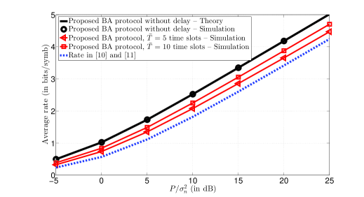
Figure 2: Achievable average rates for $M=5$, $[\Omega_{S1},\Omega_{S2},\Omega_{S3},\Omega_{S4},\Omega_{S5}]=[0.5,\;1,\;1.5,\;2,\;2.5]$, and $[\Omega_{1D},\Omega_{2D},\Omega_{3D},\Omega_{4D},\Omega_{5D}]=[3,\;1.3,\;0.9,\;1.1,\;0.7]$.

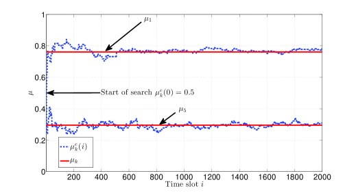
Figure 3: Estimated $\mu_{1}^{e}(i)$ and $\mu_{5}^{e}(i)$ as a function of the time slot $i$.

In Fig. 2, we plot the theoretical maximum average rate obtained from Theorem 1, and Lemmas 2 and 3, for $M=5$ relays and i.n.d. fading, where

$$[\Omega_{S1},\Omega_{S2},\Omega_{S3},\Omega_{S4},\Omega_{S5}]=[0.5,\;1,\;1.5,\;2,\;2.5]$$

and

$$\;[\Omega_{1D},\Omega_{2D},\Omega_{3D},\Omega_{4D},\Omega_{5D}]=[3,\;1.3,\;0.9,\;1.1,\;0.7].$$

We have also included simulation results for the proposed buffer-aided protocol, where the $\mu_{k}^{e}(i)$, $k=1,...,5$, are found using the recursive method in (60) with $\delta_{k}(i)=0.1/\sqrt{i}$, $\forall k$. As can be seen, the simulated average rate coincides perfectly with the theoretical average rate. As a benchmark, in Fig. 2, we show the average rate given in [10] and [11]. Moreover, we have also included the average rates achieved using the delay limited BA protocol introduced in Section V-B for an average delay of $\bar{T}=5$ and $\bar{T}=10$ time slots. For the delay limited protocol, in order to evaluate (67) we have used $\lambda_{k}(1)=0.9$ and the step size function $\zeta_{k}(i)=0.005/\sqrt{i}/\log_{2}(1+P/\sigma_{n}^{2})$, $\forall k$. As can be seen from Fig. 2, both the delay-unlimited and the delay-limited BA protocols achieve higher rates than the rate achieved in [10] and [11]. We note that we cannot use the protocols in [8] and [9] as benchmarks in Fig. 2 since these protocols are not applicable in i.n.d. fading as the buffers would become unstable. In particular, for the protocols in [8] and [9], the buffers at relays with $\Omega_{Sk}>\Omega_{kD}$ would suffer from overflow and receive more information than they can transmit. Hence, a fraction of the source’s data would be trapped inside the buffers and does not reach the destination, i.e., data loss would occur.

For the parameters adopted in Fig. 2, we show in Fig. 3 the corresponding constants $\mu_{1}$ and $\mu_{5}$ obtained using Lemma 2, and the corresponding estimated parameters $\mu_{1}^{e}(i)$ and $\mu_{5}^{e}(i)$ obtained using the recursive method in (60) as functions of time for $P/\sigma_{n}^{2}=0$ dB. As can be seen from Fig. 3, the estimated parameters $\mu_{1}^{e}(i)$ and $\mu_{5}^{e}(i)$ converge relatively quickly to $\mu_{1}$ and $\mu_{5}$, respectively.

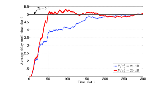
Figure 4: Average delay until time slot $i$ for $T_{0}=5$ and different $P/\sigma_{n}^{2}$ .

Furthermore, for the parameters adopted in Fig. 2, we have plotted the average delay of the proposed delay-limited protocol until time slot $i$ in Fig. 4, for the case when $T_{0}=5$ time slots, and $P/\sigma_{n}^{2}=20$ dB and $P/\sigma_{n}^{2}=25$ dB. The average delay until time slot $i$ is computed based on (64) where the queue size and the arrival rates are averaged over the time window from the first time slot to the $i$-th time slot. Hence, for finite $i$, the average delay until time slot $i$ is the average of a random process over a time window of limited duration. Because of the assumed ergodicity, for $i\to\infty$, the size of the averaging window becomes infinite and the time average converges to the mean of this random process. However, for $i<\infty$, the time average is still a random process. This is the reason for the random fluctuations in the average delay until time slot $i$ in Fig. 4. Nevertheless, Fig. 4 shows that the average delay until time slot $i$ converges relatively fast to $T_{0}$ as $i$ increases. Moreover, after the average delay has reached $T_{0}$, it exhibits relatively small fluctuations around $T_{0}$.

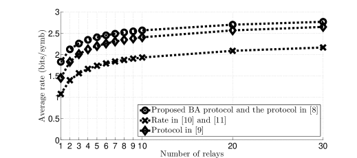
Figure 5: Achievable average rates for $\Omega_{Sk}=\Omega_{kD}=1$, $\forall k$, as a function of the number of relays $M$.

In Fig. 5, we plot the theoretical achievable average rates for BA relaying for i.i.d. fading with $\Omega_{Sk}=\Omega_{kD}=1$, $\forall k$, and $P/\sigma_{n}^{2}=10$ dB, as a function of the number of relays $M$. As can be seen from this numerical example, the growth rate of the maximum average rate is inversely proportional to $M$, i.e., the growth rate of the average data rate decreases as $M$ increases. In particular, the largest increase in data rate is observed when $M$ increases from one to two relays, whereas the increase in the maximum average rate when $M$ increases from 29 to 30 relays is almost negligible. This behavior can be most clearly seen from the expression for the average rate for low SNR given in (54). According to (54), the average rate increases proportionally to $1+1/2+1/3+...+1/(2M)$. Therefore, when $M$ is large, adding one more relay to the network has a negligible effect on the average rate. As benchmarks, we also show the average rate given in [10] and [11], and the average rates achieved with the protocols in [8] and [9]. For i.i.d. links, as explained in Remark 1, the protocol in [8] is identical to the protocol presented in Theorem 1, thereby leading to the same rate.

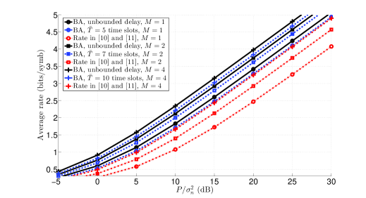
Figure 6: Achievable average rates for $\Omega_{Sk}=\Omega_{kD}=1$, $\forall k$, vs $P/\sigma_{n}^{2}$ for different number of relays $M$, and different delay.

In Fig. 6, we plot the achievable average rate for BA relaying without and with a delay constraint, as a function of $P/\sigma_{n}^{2}$, for i.i.d. fading and different numbers of relays $M$. This numerical example shows that, as the number of relays increases, the permissible average delay has to be increased in order for the rate of the delay constrained protocol to approach the rate of the non-delay constrained protocol. More precisely, for a single relay network, an average delay of five time slots is sufficient for the rate of the delay constrained protocol to approach the rate of the non-delay constrained protocol. However, for a network with two and four relays, the corresponding required delays are $7$ and $10$ time slots, respectively. For comparison, we have also plotted the average rate given in [10] and [11], which requires a delay of one time slot. Fig. 6 shows that the average rate of the buffer-aided relaying protocol with five time slots delay and only one relay surpasses the average rate in [10] and [11] for four relays.

VII Conclusion

We have devised buffer-aided relaying protocols for the slow fading HD relay selection network and derived the corresponding achievable average rates. We have proposed a buffer-aided protocol which maximizes the achievable average rate but introduces an unbounded delay, and a buffer-aided protocol which bounds the average delay at the expense of a decrease in rate. We have shown that the new achievable rates are larger than the rates achieved with existing relay selection protocols. We have also provided centralized and distributed implementations of the proposed buffer-aided protocols, which do not cause more signaling overhead than conventional relay selection protocols for adaptive rate transmission and do not need any a priori knowledge of the statistics of the involved channels.

-A Proof of Lemma 1

We denote the left and right hand sides of (19) as $A_{k}$ and $D_{k}$, respectively, i.e.,

$$A_{k} =\lim_{N\to\infty}\frac{1}{N}\sum_{i=1}^{N}r_{k}^{\rm R}(i)C_{Sk}(i),$$ (70)

$$D_{k} =\lim_{N\to\infty}\frac{1}{N}\sum_{i=1}^{N}r_{k}^{\rm T}(i)C_{kD}(i).$$ (71)

There are three possible cases for the relationship between $A_{k}$ and $D_{k}$, i.e., $A_{k}>D_{k}$, $A_{k}<D_{k}$, and $A_{k}=D_{k}$. If $A_{k}>D_{k}$ then the buffer of the $k$-th relay is receiving more information than it transmits. Therefore, the average queue length in the buffer grows with time to infinity, and, as a result, $\bar{R}_{kD}=D_{k}$, for a proof please refer to [27, Section 1.5]. Whereas, if $A_{k}<D_{k}$, due to the conservation of flow, the buffer cannot emit more information than it receives, and therefore $\bar{R}_{kD}=A_{k}$. We now prove that for $A_{k}>D_{k}$ and $A_{k}<D_{k}$, $\bar{R}_{kD}$ can always be increased by changing the values of $r_{k}^{\rm R}(i)$ and $r_{k}^{\rm T}(i)$. As a result, the only remaining possibility is that $\bar{R}_{SD}$ is maximized for $A_{k}=D_{k}$. Furthermore, since the achievable rate is given by $\bar{R}_{SD}=\sum_{k=1}^{M}\bar{R}_{kD}$, if $\bar{R}_{kD}$ increases, $\bar{R}_{SD}$ will also increase.

Assume first that $A_{k}>D_{k}$. Then, we can always increase $D_{k}$, and thereby increase $\bar{R}_{kD}$, by switching any $r_{k}^{\rm R}(i)=1$ for which $Q_{k}(i-1)>0$ holds, from one to zero and, for the same $i$, switch $r_{k}^{\rm T}(i)$ from zero to one. On the other hand, if $A_{k}<D_{k}$ then we can always increase $A_{k}$, and thereby increase $\bar{R}_{kD}$, by switching any randomly chosen $r_{k}^{\rm T}(i)=1$ from one to zero and, for the same $i$, switch $r_{k}^{\rm R}(i)$ from zero to one. Now, since $\bar{R}_{SD}$ can always be improved when $A_{k}>D_{k}$ or $A_{k}<D_{k}$, it follows that $\bar{R}_{SD}$ is maximized for $A_{k}=D_{k}$. Furthermore, when the $\bar{R}_{kD}$ are maximized $\forall k$, then $\bar{R}_{SD}$ is also maximized. Moreover, for $A_{k}=D_{k}$ the buffer at the $k$-th relay is stable since the information that arrives at the buffer also leaves the buffer without information loss. On the other hand, the proof that (20) holds when (19) is satisfied is given in [13, Appendix B]. Finally, considering (III-B), if (20) holds $\forall k$, then (21) holds as well. This concludes the proof.

-B Proof of Theorem 1

To solve (28), we first relax the binary constraints $r_{k}^{\rm T}(i)\in\{0,1\}$ and $r_{k}^{\rm R}(i)\in\{0,1\}$ in (28) to $0\leq r_{k}^{\rm T}(i)\leq 1$ and $0\leq r_{k}^{\rm R}(i)\leq 1$, $\forall i$, respectively. Thereby, we transform the original problem (28) into the following linear optimization problem

$$\begin{array}[]{ll}{\underset{r_{k}^{\rm R}(i),r_{k}^{\rm T}(i),\forall i,k}{\rm{Maximize:}}}&\frac{1}{N}\sum_{i=1}^{N}\sum_{k=1}^{M}r_{k}^{\rm T}(i)C_{kD}(i)\\ \vspace{1mm}{\rm{Subject\;\;to:}}&{\rm C1:}\,\frac{1}{N}\sum_{i=1}^{N}r_{k}^{\rm R}(i)C_{Sk}(i)\\ &\qquad=\frac{1}{N}\sum_{i=1}^{N}r_{k}^{\rm T}(i)C_{kD}(i),\;\forall k\\ \vspace{1mm}&{\rm C2:}\,0\leq r_{k}^{\rm R}(i)\leq 1,\;\forall k,i\\ \vspace{1mm}&{\rm C3:}\,0\leq r_{k}^{\rm T}(i)\leq 1,\;\forall k,i\\ \vspace{1mm}&{\rm C4:}\,0\leq\sum_{k=1}^{M}[r_{k}^{\rm R}(i)+r_{k}^{\rm T}(i)]\leq 1,\;\forall k,i.\\ \end{array}$$ (78)

In the following, we solve the relaxed problem (78) and then show that the optimal values of $r_{k}^{\rm T}(i)$ and $r_{k}^{\rm R}(i)$, $\forall i,k$ are at the boundaries, i.e., $r_{k}^{\rm R}(i)\in\{0,1\}$ and $r_{k}^{\rm T}(i)\in\{0,1\}$, $\forall i,k$. Therefore, the solution of the relaxed problem (78) is also the solution to the original maximization problem in (28).

Since (78) is a linear optimization problem, we can solve it by using the method of Lagrange multipliers. The Lagrangian function for maximization problem (78) is given by

$$\mathcal{L} =\sum_{k=1}^{M}\frac{1}{N}\sum_{i=1}^{N}r_{k}^{\rm T}(i)C_{kD}(i)$$

$$-\sum_{k=1}^{M}\mu_{k}\left(\frac{1}{N}\sum_{i=1}^{N}r_{k}^{\rm T}(i)C_{kD}(i)-\frac{1}{N}\sum_{i=1}^{N}r_{k}^{\rm R}(i)C_{Sk}(i)\right)$$

$$-\sum_{k=1}^{M}\frac{1}{N}\sum_{i=1}^{N}\alpha_{k}^{\rm T}(i)\left(r_{k}^{\rm T}(i)-1\right)+\sum_{k=1}^{M}\frac{1}{N}\sum_{i=1}^{N}\beta_{k}^{\rm T}(i)r_{k}^{\rm T}(i)$$

$$-\sum_{k=1}^{M}\frac{1}{N}\sum_{i=1}^{N}\alpha_{k}^{\rm R}(i)\left(r_{k}^{\rm R}(i)-1\right)+\sum_{k=1}^{M}\frac{1}{N}\sum_{i=1}^{N}\beta_{k}^{\rm R}(i)r_{k}^{\rm R}(i)$$

$$-\frac{1}{N}\sum_{i=1}^{N}\phi(i)\left(\sum_{k=1}^{M}[r_{k}^{\rm R}(i)+r_{k}^{\rm T}(i)]-1\right)$$

$$+\frac{1}{N}\sum_{i=1}^{N}\lambda(i)\left(\sum_{k=1}^{M}[r_{k}^{\rm R}(i)+r_{k}^{\rm T}(i)]\right),$$ (79)

where $\mu_{k}/N$, $\alpha_{k}^{x}(i)/N$, $\beta_{k}^{x}(i)/N$, for $x\in\{\rm R,T\}$, $\phi(i)/N$, and $\lambda(i)/N$ are Lagrange multipliers. These multipliers have to satisfy the following conditions.

1)   Dual feasibility condition: The Lagrange multipliers for the inequality constraints have to be non-negative, i.e.,

$$\alpha_{k}^{\rm R}(i)\geq 0,\;\alpha_{k}^{\rm T}(i)\geq 0,\;\beta_{k}^{\rm R}(i)\geq 0,\;\beta_{k}^{\rm T}(i)\geq 0,$$

$$\phi(i)\geq 0,\;\lambda(i)\geq 0,\quad\forall i,k.$$ (80)

have to hold.
2)   Complementary slackness condition: If an inequality is inactive, i.e., the optimal solution is in the interior of the corresponding set, the corresponding Lagrange multipliers are zero. Therefore, we obtain

$$\alpha_{k}^{\rm R}(i)\left(r_{k}^{\rm R}-1\right)=0,\quad\alpha_{k}^{\rm T}(i)\left(r_{k}^{\rm T}-1\right)=0,\quad\forall i,k$$ (81)

$$\beta_{k}^{\rm R}(i)r_{k}^{\rm R}=0,\quad\beta_{k}^{\rm T}(i)r_{k}^{\rm T}=0,\quad\forall i,k$$ (82)

$$\phi(i)\left(\sum_{k=1}^{M}[r_{k}^{\rm R}(i)+r_{k}^{\rm T}(i)]-1\right)=0,$$

$$\lambda(i)\left(\sum_{k=1}^{M}[r_{k}^{\rm R}(i)+r_{k}^{\rm T}(i)]\right)=0,\quad\forall i,k.$$ (83)

We now differentiate the Lagrangian function with respect to $r_{n}^{\rm R}(i)$ and $r_{m}^{\rm T}(i)$, for $n\in\{1,...,M\}$ and $m\in\{1,...,M\}$, and equate the results to zero, respectively. This leads to the following two equations

$$\mu_{n}C_{Sn}(i) =\alpha_{n}^{\rm R}(i)-\beta_{n}^{\rm R}(i)+\phi(i)-\lambda(i)$$ (84)

$$\left(1-\mu_{m}\right)C_{mD}(i) =\alpha_{m}^{\rm T}(i)-\beta_{m}^{\rm T}(i)+\phi(i)-\lambda(i).$$ (85)

We first show that for the optimal solution of $r_{n}^{\rm R}(i)$ and $r_{m}^{\rm R}(i)$, $0<r_{n}^{\rm R}(i)<1$ and/or $0<r_{m}^{\rm T}(i)<1$ cannot hold for any $n,m\in\{1,...,M\}$, and only $r_{n}^{\rm R}(i)\in\{0,1\}$ and $r_{m}^{\rm T}(i)\in\{0,1\}$ can hold $\forall n,m=1,...,M$. We prove this by contradiction. Assume that $0<r_{n}^{\rm R}(i)<1$ and $0<\sum_{k=1}^{M}[r_{k}^{\rm R}(i)+r_{k}^{\rm T}(i)]<1$. Then, according to (81), $\alpha_{n}^{\rm R}(i)=\beta_{n}^{\rm R}(i)=\phi(i)=\lambda(i)=0$ must hold. Inserting this into (84a), we obtain

$$\mu_{n}C_{Sn}(i)=0.$$ (86)

Since $C_{Sn}(i)$ is an RV, (86) can hold only for $\mu_{n}=0$. However, if we assume $\mu_{n}=0$, and insert $\mu_{n}=0$ in (84b) by setting $m=n$, we obtain

$$C_{nD}(i)=\alpha_{n}^{\rm T}(i)-\beta_{n}^{\rm T}(i).$$ (87)

Since $C_{nD}(i)$ is a non-negative RV, and since either $\alpha_{n}^{\rm T}(i)$ or $\beta_{n}^{\rm T}(i)$ can be larger than zero but not both, in order for (87) to hold, $\beta_{n}^{\rm T}(i)$ must be zero and $\alpha_{n}^{\rm T}(i)=C_{nD}(i)$. On the other hand, if $\beta_{n}^{\rm T}(i)=0$, it would mean that $r_{n}^{\rm T}(i)=1$. However, if $r_{n}^{\rm T}(i)=1$ and $0<r_{n}^{\rm R}(i)<1$ hold jointly, this would violate our starting assumption that $0<\sum_{k=1}^{M}[r_{k}^{\rm R}(i)+r_{k}^{\rm T}(i)]<1$ holds. Hence, $0<r_{n}^{\rm R}(i)<1$ and $0<\sum_{k=1}^{M}[r_{k}^{\rm R}(i)+r_{k}^{\rm T}(i)]<1$ cannot hold.

Now, let us assume that $0<r_{n}^{\rm R}(i)<1$ and $\sum_{k=1}^{M}[r_{k}^{\rm R}(i)+r_{k}^{\rm T}(i)]=1$. Since $r_{n}^{\rm R}(i)<1$, then at least one other variable $r_{k}^{\rm R}(i)$ or $r_{m}^{\rm T}(i)$ has to be larger than zero but smaller than one, where $k\in\{1,...,M\},\;\;k\neq n$, and $m\in\{1,...,M\}$. Let us assume that this variable is $r_{k}^{\rm R}(i)$, where $k\neq n$. Hence, $0<r_{k}^{\rm R}(i)<1$, for $k\neq n$. Then, according to (81), $\alpha_{n}^{\rm R}(i)=\beta_{n}^{\rm R}(i)=\alpha_{k}^{\rm R}(i)=\beta_{k}^{\rm R}(i)=\lambda(i)=0$, and $\phi(i)\geq 0$ must hold. Inserting these values in (84a), we obtain

$$\mu_{n}C_{Sn}(i)=\phi(i)=\mu_{k}C_{Sk}(i).$$ (88)

However, since $C_{Sn}(i)$ and $C_{Sk}(i)$ are independent RVs, (88) cannot hold for any arbitrarily chosen $i$. On the other hand, if we assume that instead of $r_{k}^{\rm R}(i)$, the variable which is larger than one is $r_{k}^{\rm T}(i)$, we would have obtained that

$$\mu_{n}C_{Sn}(i)=\phi(i)=(1-\mu_{k})C_{kD}(i)$$ (89)

must hold. Since (89) also cannot hold for any arbitrarily chosen $i$, we obtain that $0<r_{n}^{\rm R}(i)<1$ and $\sum_{k=1}^{M}[r_{k}^{\rm R}(i)+r_{k}^{\rm T}(i)]=1$ cannot hold. Therefore, the only other possibility is that $r_{n}^{\rm R}(i)\in\{0,1\}$ must hold.

Following the same approach as above, we can also prove that $r_{m}^{\rm T}(i)\in\{0,1\}$ must hold. Moreover, due to constraint C4 in (78), it is clear that if $r_{n}^{\rm R}(i)=1$, for any $n\in\{1,...,M\}$, then $r_{k}^{\rm R}(i)=0$ for all $k=1,...,M$, $k\neq n$, and $r_{m}^{\rm T}(i)=0$ for all $m=1,...,M$ must hold. Similarly, if $r_{m}^{\rm T}(i)=1$, for any $m\in\{1,...,M\}$, then $r_{k}^{\rm T}(i)=0$ for all $k=1,...,M$, $k\neq m$, and $r_{n}^{\rm R}(i)=0$ for all $n=1,...,M$ must hold. In the following, we investigate the conditions under which $r_{n}^{\rm R}(i)=1$ and all other $r_{k}^{\rm R}(i)=0$ for $k=1,...,M$, $k\neq n$, and all other $r_{m}^{\rm T}(i)=0$ for $m=1,...,M$.

Assume $r_{n}^{\rm R}(i)=1$. Then, $r_{k}^{\rm R}(i)=0$ for $k=1,...,M$, $k\neq n$, and $r_{m}^{\rm T}(i)=0$ for $m=1,...,M$ must hold. As a result, according to (81), $\alpha^{\rm R}_{n}(i)\geq 0$, $\beta^{\rm R}_{k}(i)\geq 0$, $\beta^{\rm T}_{m}(i)\geq 0$, $\phi(i)\geq 1$, and $\beta_{n}^{\rm R}(i)=\alpha^{\rm R}_{k}(i)=\alpha^{\rm R}_{m}(i)=\lambda(i)=0$ must hold, for $k=1,...,M$, $k\neq n$, and $m=1,...,M$. Inserting these variables in (84), we obtain the following

$$\mu_{n}C_{Sn}(i) \;=\; \alpha^{\rm R}_{n}(i)+\phi(i),$$ (90)

$$\mu_{k}C_{Sk}(i) \;=\; -\beta^{\rm R}_{k}(i)+\phi(i),\;\forall k\neq n$$ (91)

$$(1-\mu_{m})C_{mD}(i) \;=\; -\beta^{\rm T}_{m}(i)+\phi(i),\;\forall m.$$ (92)

Subtracting (91) from (90) and subtracting (92) from (90), we obtain

$$\mu_{n}C_{Sn}(i)-\mu_{k}C_{Sk}(i) =\alpha^{\rm R}_{n}(i)+\beta^{\rm R}_{k}(i),\;\forall k\neq n$$ (93)

$$\mu_{n}C_{Sn}(i)-(1-\mu_{m})C_{mD}(i) =\alpha^{\rm R}_{n}(i)+\beta^{\rm R}_{m}(i),\;\forall m.$$ (94)

Since $\alpha^{\rm R}_{n}(i)+\beta^{\rm R}_{k}(i)\geq 0$ and $\alpha^{\rm R}_{n}(i)+\beta^{\rm R}_{m}(i)\geq 0$ hold, it follows that $r_{n}^{\rm R}(i)=1$ when the following holds

$$\mu_{n}C_{Sn}(i)>\mu_{k}C_{Sk}(i),\;\forall k\neq n$$

$$\textrm{ AND }\mu_{n}C_{Sn}(i)>(1-\mu_{m})C_{mD}(i),\;\forall m.$$ (95)

Eq. (95) can be written in compact form as

$$r_{k}^{\rm R}(i)=1 \textrm{if }\;\mu_{k}C_{Sk}(i)=\max\mathcal{A}(i),$$ (96)

where set $\mathcal{A}(i)$ is defined in (III-C). Following the same approach as above, we can prove that

$$r_{k}^{\rm T}(i)=1 \textrm{if }\;(1-\mu_{k})C_{kD}(i)=\max\mathcal{A}(i).$$ (97)

Combining (96) and (97), we obtain (33). This completes the proof of Theorem 1.

-C Proof of Lemma 2

The optimal $\mu_{k}$, $\forall k$, are found from the system of $M$ equations given in (38). Using the definition of the expected value, (38) can be written equivalently as (44), where the RVs $\Gamma_{Sk}$ and $\Gamma_{kD}$ are given by

$$\Gamma_{Sk} = \left\{\begin{array}[]{cl}\gamma_{Sk}&\textrm{if }\mu_{k}C_{Sk}=\max\mathcal{A}\\ 0&\textrm{if }\mu_{k}C_{Sk}\neq\max\mathcal{A}\end{array}\right.,$$ (100)

$$\Gamma_{kD} = \left\{\begin{array}[]{cl}\gamma_{kD}&\textrm{if }(1-\mu_{k})C_{kD}=\max\mathcal{A}\\ 0&\textrm{if }(1-\mu_{k})C_{kD}\neq\max\mathcal{A}.\end{array}\right.$$ (103)

Hence, to find the optimal $\mu_{k}$, $\forall k$, we only have to find the PDFs of $\Gamma_{Sk}$ and $\Gamma_{kD}$, $f_{\Gamma_{Sk}}(x)$ and $f_{\Gamma_{kD}}(x)$, and insert them into (44). In the following, we first derive the PDF of $\Gamma_{Sk}$.

Using (100), we can obtain the PDF of $\Gamma_{Sk}$, $f_{\Gamma_{Sk}}(x)$, for $x>0$, as

$$f_{\Gamma_{Sk}}(x)=f_{\gamma_{Sk}}(x){\rm Pr}\big{\{}\mu_{k}C_{Sk}=\max\mathcal{A}\big{\}},\;\;x>0,$$ (104)

where $\rm{Pr}\{\cdot\}$ denotes probability. Note that the distribution of $f_{\Gamma_{Sk}}(x)$ for $x=0$, is not needed for the computation of the expectations in (38) and (39). The only unknown in (104) is the probability ${\rm Pr}\big{\{}\mu_{k}C_{Sk}=\max\mathcal{A}\big{\}}$. In the following, we derive this probability. To this end, we set $\gamma_{Sk}=x$, and obtain

$${\rm Pr}\big{\{}\mu_{k}C_{Sk}=\max\mathcal{A}\big{\}}={\rm Pr}\big{\{}\mu_{k}\log_{2}(1+x)=\max\mathcal{A}\big{\}}$$

$$=\prod_{j=1,j\neq k}^{M}{\rm Pr}\left\{\mu_{j}\log_{2}(1+\gamma_{Sj})<\mu_{k}\log_{2}(1+x)\right\}$$

$$\times\prod_{j=1}^{M}{\rm Pr}\left\{(1-\mu_{j})\log_{2}(1+\gamma_{jD})<\mu_{k}\log_{2}(1+x)\right\}$$

$$=\prod_{j=1,j\neq k}^{M}{\rm Pr}\left\{\gamma_{Sj}<(1+x)^{\frac{\mu_{k}}{\mu_{j}}}-1\right\}$$

$$\times\prod_{j=1}^{M}{\rm Pr}\left\{\gamma_{jD}<(1+x)^{\frac{\mu_{k}}{1-\mu_{j}}}-1\right\}$$

$$=\prod_{j=1,j\neq k}^{M}F_{\gamma_{Sj}}\left((1+x)^{\frac{\mu_{k}}{\mu_{j}}}-1\right)$$

$$\times\prod_{j=1}^{M}F_{\gamma_{jD}}\left((1+x)^{\frac{\mu_{k}}{1-\mu_{j}}}-1\right),$$ (105)

where $F_{\gamma_{\alpha}}(x)$ is the CDF of $\gamma_{\alpha}$, for $\alpha\in\{Sk,kD\}$. Inserting (105) into (104), we obtain (45). Following a similar procedure as above, we obtain the distribution of $\Gamma_{kD}$ given in (46).

Now, assume that all source-to-relay and relay-to-destination links are i.i.d. Then, $f_{\gamma_{Sk}}(x)=f_{\gamma_{kD}}(x)=f_{\gamma}(x)$ holds $\forall k$. Moreover, $F_{\gamma_{Sk}}(x)=F_{\gamma_{kD}}(x)=F_{\gamma}(x)$ also holds $\forall k$. As a result, (45) and (46) can be written for $x>0$ as

$$f_{\Gamma_{Sk}}(x)=f_{\gamma}(x)F_{\gamma}\left((1+x)^{\frac{\mu_{k}}{1-\mu_{k}}}-1\right)$$

$$\times\prod_{\underset{j\neq k}{j=1}}^{M}F_{\gamma}\left((1+x)^{\frac{\mu_{k}}{\mu_{j}}}-1\right)F_{\gamma}\left((1+x)^{\frac{\mu_{k}}{1-\mu_{j}}}-1\right),$$ (106)

$$f_{\Gamma_{kD}}(x)=f_{\gamma}(x)F_{\gamma}\left((1+x)^{\frac{1-\mu_{k}}{\mu_{k}}}-1\right)$$

$$\times\prod_{\underset{j\neq k}{j=1}}^{M}F_{\gamma}\left((1+x)^{\frac{1-\mu_{k}}{\mu_{j}}}-1\right)F_{\gamma}\left((1+x)^{\frac{1-\mu_{k}}{1-\mu_{j}}}-1\right).$$ (107)

We observe that $f_{\Gamma_{Sk}}(x)$ and $f_{\Gamma_{kD}}(x)$ in (106) and (107), respectively, are both functions of $\mu_{k}$ and show this explicitly by redefining them as $f_{\Gamma_{Sk}}(x,\mu_{k})$ and $f_{\Gamma_{kD}}(x,\mu_{k})$, respectively. Moreover, from (106) and (107) we observe that

$$f_{\Gamma_{kD}}(x,\mu_{k})=f_{\Gamma_{Sk}}(x,1-\mu_{k})$$ (108)

holds. If we now insert (108) into (44), we obtain

$$\int_{0}^{\infty}\log_{2}(1+x)f_{\Gamma_{Sk}}(x,\mu_{k})dx$$

$$=\int_{0}^{\infty}\log_{2}(1+x)f_{\Gamma_{Sk}}(x,1-\mu_{k})dx,\;\forall k=1,...,M.$$ (109)

Now, observe that (-C) holds if and only if $\mu_{k}=1-\mu_{k}$, which leads to $\mu_{k}=1/2$. This concludes the proof.

-D Proof of Lemma 4

The average delay for a system with $M$ parallel queues is well known, and given by [28, Eq. 11.69]. After changing the notations in [28, Eq. 11.69] to our notations, we directly obtain (64). In the following, we give an alternative, more intuitive proof of (64).

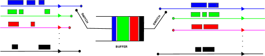
Figure 7: Equivalent single buffer model.

The input-output dynamics at the $M$ buffers in the considered network during $N$ time slots can be represented equivalently by a single buffer model, shown in Fig. 7. The different colors in this model correspond to the information bits which are received/transmitted by the different relays. For example, the blue, green, and red colors correspond to the bits that are send/received via relay 1, 2, and 3, respectively. In this model, the buffer is filled in the same order as the order of the packets that arrive at the buffers at the different relays. Which packet arrives at the equivalent buffer depends on the position of the input switch in each time slot, which on the other hand, depends on the values of $r_{k}^{\rm R}(i)$, $\forall i,k$. The extraction of the bits from the equivalent buffer also depends on the position of the output switch in each time slot, which on the other hand, depends on the values of $r_{k}^{\rm T}(i)$, $\forall i,k$. Moreover, when the output switch is set to a line with a specific color, only bits with that color are extracted from the equivalent buffer. Hence, the extraction order is different from the order of filling the equivalent buffer. Nevertheless, since the average delay computed by Little’s formula [29], is independent of the order of extracting from the buffer, see [30, pp. 89-91], for the system model in Fig. 7, the average delay $\bar{T}$ can be computed as [29]

$$\bar{T}=\frac{\bar{Q}_{\rm eq}}{\bar{A}_{\rm eq}},$$ (110)

where $\bar{Q}_{\rm eq}$ is the average queue size of the equivalent buffer and $\bar{A}_{\rm eq}$ is the average arrival rate of the equivalent buffer. Now, using the fact that $\bar{Q}_{\rm eq}=\sum_{k=1}^{M}\bar{Q}_{k}$ and $\bar{A}_{\rm eq}=\sum_{k=1}^{M}\bar{R}_{Sk}$, we obtain (64). This concludes the proof.

Nikola Zlatanov (S’06) was born in Macedonia. He received his Dipl.Ing. and M.S. degrees in electrical engineering from SS. Cyril and Methodius University, Skopje, Macedonia, in 2007 and 2010, respectively. Currently, he is working toward his Ph.D. degree at the University of British Columbia (UBC), Vancouver, Canada. His current research interests include wireless communications and information theory. Mr. Zlatanov received several awards for his work including UBC’s Four-Year Doctoral Fellowship in 2010, UBC’s Killam Doctoral Scholarship and Macedonia’s Young Scientist of the Year Award in 2011, Vanier Canada Graduate Scholarship in 2012, DAAD Research Grant in 2013, and best paper award from the German Information Technology Society (ITG) in 2014.

Vahid Jamali (S’12) was born in Fasa, Iran, in 1988. He received his B.S. and M.S. degrees in electrical engineering from K. N. Toosi University of Technology (KNTU), in 2010 and 2012, respectively. Currently, he is working toward his Ph.D. degree at the Friedrich-Alexander University (FAU), Erlangen, Germany. His research interests include multiuser information theory, wireless communications, cognitive radio network, LDPC codes, and optimization theory.

Robert Schober (S’98, M’01, SM’08, F’10) was born in Neuendettelsau, Germany, in 1971. He received the Diplom (Univ.) and the Ph.D. degrees in electrical engineering from the University of Erlangen-Nuermberg in 1997 and 2000, respectively. From May 2001 to April 2002 he was a Postdoctoral Fellow at the University of Toronto, Canada, sponsored by the German Academic Exchange Service (DAAD). Since May 2002 he has been with the University of British Columbia (UBC), Vancouver, Canada, where he is now a Full Professor. Since January 2012 he is an Alexander von Humboldt Professor and the Chair for Digital Communication at the Friedrich Alexander University (FAU), Erlangen, Germany. His research interests fall into the broad areas of Communication Theory, Wireless Communications, and Statistical Signal Processing. Dr. Schober received several awards for his work including the 2002 Heinz Maier-Leibnitz Award of the German Science Foundation (DFG), the 2004 Innovations Award of the Vodafone Foundation for Research in Mobile Communications, the 2006 UBC Killam Research Prize, the 2007 Wilhelm Friedrich Bessel Research Award of the Alexander von Humboldt Foundation, the 2008 Charles McDowell Award for Excellence in Research from UBC, a 2011 Alexander von Humboldt Professorship, and a 2012 NSERC E.W.R. Steacie Fellowship. In addition, he received best paper awards from the German Information Technology Society (ITG), the European Association for Signal, Speech and Image Processing (EURASIP), IEEE WCNC 2012, IEEE Globecom 2011, IEEE ICUWB 2006, the International Zurich Seminar on Broadband Communications, and European Wireless 2000. Dr. Schober is a Fellow of the Canadian Academy of Engineering and a Fellow of the Engineering Institute of Canada. He is currently the Editor-in-Chief of the IEEE Transactions on Communications.

References

- [1] A. Bletsas, A. Khisti, D. Reed, and A. Lippman, “A Simple Cooperative Diversity Method Based on Network Path Selection,” IEEE J. Select. Areas Commun., vol. 24, pp. 659–672, Mar. 2006.
- [2] S. Cui, A. Haimovich, O. Somekh, and H. Poor, “Opportunistic Relaying in Wireless Networks,” IEEE Trans. Inform. Theory, vol. 55, pp. 5121–5137, Nov. 2009.
- [3] M. Fareed and M. Uysal, “On Relay Selection for Decode-and-Forward Relaying,” IEEE Trans. Wireless Commun., vol. 8, pp. 3341–3346, Jul. 2009.
- [4] Y. Jing and H. Jafarkhani, “Single and Multiple Relay Selection Schemes and Their Achievable Diversity Orders,” IEEE Trans. Wireless Commun., vol. 8, pp. 1414–1423, Mar. 2009.
- [5] D. Michalopoulos and G. Karagiannidis, “Performance Analysis of Single Relay Selection in Rayleigh Fading,” IEEE Trans. Wireless Commun., vol. 7, pp. 3718–3724, Oct. 2008.
- [6] R. Tannious and A. Nosratinia, “Spectrally-Efficient Relay Selection with Limited Feedback,” IEEE J. Select. Areas Commun., vol. 26, no. 8, pp. 1419–1428, Oct. 2008.
- [7] Z. Yi and I.-M. Kim, “Diversity Order Analysis of the Decode-and-Forward Cooperative Networks with Relay Selection,” IEEE Trans. Wireless Commun., vol. 7, no. 5, pp. 1792–1799, May 2008.
- [8] I. Krikidis, T. Charalambous, and J. Thompson, “Buffer-Aided Relay Selection for Cooperative Diversity Systems without Delay Constraints,” IEEE Trans. Wireless Commun., vol. 11, pp. 1957–1967, May 2012.
- [9] A. Ikhlef, D. S. Michalopoulos, and R. Schober, “Max-Max Relay Selection for Relays with Buffers,” IEEE Trans. Wireless Commun., vol. 11, pp. 1124–1135, Mar. 2012.
- [10] A. Adinoyi, Y. Fan, H. Yanikomeroglu, H. Poor, and F. Al-Shaalan, “Performance of Selection Relaying and Cooperative Diversity,” IEEE Trans. Wireless Commun., vol. 8, pp. 5790–5795, Dec. 2009.
- [11] S. Ikki and M. Ahmed, “Performance Analysis of Adaptive Decode-and-Forward Cooperative Diversity Networks with Best-Relay Selection,” IEEE Trans. Commun., vol. 58, pp. 68–72, Jan. 2010.
- [12] N. Zlatanov, R. Schober, and P. Popovski, “Throughput and Diversity Gain of Buffer-Aided Relaying,” in IEEE Global Telecommunic. Conference (GLOBECOM 2011), Dec. 2011.
- [13] ——, “Buffer-Aided Relaying with Adaptive Link Selection,” IEEE J. Select. Areas Commun., vol. 31, pp. 1530–1542, 2013.
- [14] N. Zlatanov and R. Schober, “Buffer-Aided Relaying With Adaptive Link Selection - Fixed and Mixed Rate Transmission,” IEEE Trans. Inform. Theory, vol. 59, pp. 2816–2840, May 2013.
- [15] H. Liu, P. Popovski, E. de Carvalho, and Y. Zhao, “Sum-rate optimization in a two-way relay network with buffering,” IEEE Commun. Letters, vol. 17, no. 1, pp. 95–98, 2013.
- [16] V. Jamali, N. Zlatanov, A. Ikhlef, and R. Schober, “Achievable Rate Region of the Bidirectional Buffer-Aided Relay Channel With Block Fading,” IEEE Trans. Inform. Theory, vol. 60, pp. 7090–7111, Nov. 2014.
- [17] C. Dong, L.-L. Yang, and L. Hanzo, “Performance Analysis of Multihop-Diversity-Aided Multihop Links,” IEEE Trans. Veh. Technol., vol. 61, pp. 2504–2516, Jul. 2012.
- [18] A. Zafar, M. Shaqfeh, M.-S. Alouini, and H. Alnuweiri, “Resource Allocation for Two Source-Destination Pairs Sharing a Single Relay with a Buffer,” IEEE Trans. Commun., vol. 62, pp. 1444–1457, May 2014.
- [19] J. Huang and A. Swindlehurst, “Buffer-Aided Relaying for Two-Hop Secure Communication,” IEEE Trans. Wireless Commun., vol. 14, pp. 152–164, Jan. 2015.
- [20] G. Chen, Z. Tian, Y. Gong, Z. Chen, and J. Chambers, “Max-Ratio Relay Selection in Secure Buffer-Aided Cooperative Wireless Networks,” IEEE Trans. on Inform. Forensics and Security, vol. 9, pp. 719–729, Apr. 2014.
- [21] Z. Tian, G. Chen, Y. Gong, Z. Chen, and J. Chambers, “Buffer-Aided Max-Link Relay Selection in Amplify-and-Forward Cooperative Networks,” IEEE Trans. Veh. Technol., vol. 64, pp. 553–565, Feb 2015.
- [22] P. Deuflhard, Newton Methods for Nonlinear Problems: Affine Invariance and Adaptive Algorithms. Springer, 2011, vol. 35.
- [23] H. A. David and H. N. Nagaraja, Order Statistics. Wiley Online Library, 1970.
- [24] D. S. Michalopoulos, H. A. Suraweera, and R. Schober, “Relay Selection for Simultaneous Information Transmission and Wireless Energy Transfer: A Tradeoff Perspective,” Accepted to IEEE J. Select. Areas Commun., 2014.
- [25] S. Boyd and L. Vandenberghe, Convex Optimization. Cambridge University Press, 2004.
- [26] V. Shah, N. Mehta, and R. Yim, “Optimal Timer Based Selection Schemes,” IEEE Trans. Commun., vol. 58, no. 6, pp. 1814–1823, Jun. 2010.
- [27] D. Gross and C. Harris, Fundamentals of Queueing Theory. Wiley Interscience, 1998.
- [28] N. Mir, Computer and Communication Networks. Pearson Education, 2006.
- [29] J. D. C. Little, “A Proof of the Queueing Formula: ,” Operations Research, vol. 9, no. 3, pp. 383–388, May - Jun. 1961.
- [30] J. Little and S. Graves, “Little’s law,” in Building Intuition, ser. International Series in Operations Research and Management Science. Springer US, 2008, vol. 115, pp. 81–100.