Graviton self-energy from worldlines

Abstract

Worldline approaches, when available, often simplify and make more efficient the calculation of various observables in quantum field theories. In this contribution we first review the calculation of the graviton self-energy due to a loop of virtual particles of spin 0, 1/2 and 1, all of which have a well-known worldline description. For the case of the graviton itself, an elegant worldline description is still missing, though one can still describe it by constructing a worldline representation of the differential operators that arise in the quadratic approximation of the Einstein-Hilbert action. We have recently analyzed the latter approach, and we use it here to calculate the one-loop graviton self energy due to the graviton itself in this formalism.

1 Introduction

The worldline path integral formulation of quantum field theories provides an alternative efficient method for computing Feynman diagrams, especially in the one-loop approximation, see ref. [1] for a review. The worldline method was of particular interest to Victor, who has given various contributions to the subject. In particular, in [2] he contributed in analyzing the consequences of the one-loop graviton-photon mixing in a constant electromagnetic background [3]. The Feynman diagram describing the process is drawn in figure 1,

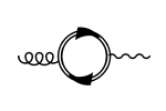
Figure 1: One-loop correction to the graviton-photon mixing due to a virtual loop of an electron in a constant magnetic field.

and constitute a prime example where the worldline approach has been used with great efficiency. The final result of that analysis was that, even for the strong magnetic fields present in our universe, the one-loop contribution amounts to no more than a few percent of the tree level mixing. However, although it is numerically only a small correction to the tree-level amplitude, unlike the tree-level amplitude the one-loop conversion of photons into gravitons in a magnetic field leads to dichroism, and surprisingly for the relevant range of parameters is even the largest standard model contribution to dichroism, as shown in [4].

Akin to the diagram of the graviton-photon mixing, there are the graviton self-energy diagrams that take place in flat spacetime (without the need of additional background fields). Those that are due to virtual particles of spin 0, 1/2 and 1 may be depicted as in figure 2,

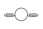
Figure 2: One-loop correction to the graviton self-energy due to particles of spin 0, 1/2 and 1 circulating in the loop.

and can be computed successfully with worldline methods. Indeed, a worldline description of particles of spin $s\leq 1$ coupled to external gravity is easily achievable, as we are going to review in the following. In particular, we outline the essential steps of the worldline calculation of the self-energy diagrams.

The description of the graviton itself is more problematic. One would like to compute in the worldline approach the diagram in figure 3, where the virtual graviton in the loop is attached to the two external gravitons.

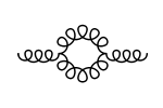
Figure 3: Graviton self-energy at one-loop due to a virtual graviton.

However, a simple and useful description of the graviton in first quantization is still missing. One may try to use the $O(4)$ spinning particle of refs. [5, 6], that indeed describes the propagation of the graviton in flat space. The problem is that it is not known how to couple that model to an external gravitational background, and the best one could do so far is to couple it to AdS spaces [7] and to conformally flat spaces [8].

Given this state of affairs, a less elegant but viable option is that of constructing a worldline representation of the differential operators that arise in the quadratic approximation of the Einstein-Hilbert action. We have recently analyzed the latter approach in [9], and we review it here. Then, we use it to compute the one-loop graviton self-energy due to the graviton itself with worldline methods.

2 The worldline formalism in gravitational backgrounds

The case of a virtual scalar particle contributing to the graviton self-energy is the simplest one, but contains already all the essential elements that enter in a worldline description of the process. It was treated in [10] to exemplify the worldline formalism in a gravitational background. To review that, one may start recalling that the action of a relativistic scalar particle in a spacetime of $D$ dimensions is proportional to the length of its worldline

$$S[x]=-m\int ds$$ (1)

where $ds=d\tau\sqrt{-\dot{x}^{\mu}\dot{x}_{\mu}}$ with $x^{\mu}(\tau)$ a generic worldline parametrized by $\tau$ and $\dot{x}^{\mu}=\frac{dx^{\mu}}{d\tau}$. The square root appearing in the action can be avoided if one uses an einbein $e(\tau)$ for the intrinsic geometry of the worldline. The action takes the form [11]

$$S[x,e]=\int d\tau\,\frac{1}{2}(e^{-1}\dot{x}^{\mu}\dot{x}_{\mu}-em^{2})$$ (2)

which has the advantage over (1) of having a smooth massless limit. This action is otherwise essentially equivalent to (1), as the equation of motion of the einbein, $e^{-2}\dot{x}^{2}+m^{2}=0$, can be solved for $m\neq 0$ by taking a positive square root to give $e=\frac{\sqrt{-\dot{x}^{2}}}{m}$. The latter plugged back into (2) produces the original action in (1). This model has a reparametrization invariance, that must be gauge-fixed upon quantization. One can show that: i) quantizing the model in flat space and choosing the topology of the worldline to be that of a segment gives the propagator of the free Klein-Gordon field, ii) quantizing the model on a closed worldline gives instead its one-loop effective action. The complication of the gauge fixing procedure, and the related emergence of an integration over a modular parameter, can be short cut as the answer must be the same as that obtained long ago by Schwinger with his proper-time representation of the propagator and one-loop effective action [12].

Let us consider the one-loop effective action in a curved background with metric $g_{\mu\nu}$. We proceed with euclidean conventions obtained after a Wick rotation to euclidean times. The classical particle action (2), Wick rotated and coupled to the background metric $g_{\mu\nu}$, is

$$S[x,e]=\int_{0}^{1}d\tau\,\frac{1}{2}\left(e^{-1}g_{\mu\nu}(x)\dot{x}^{\mu}\dot{x}^{\nu}+e(m^{2}+\xi R(x))\right)$$ (3)

where an arbitrary non-minimal coupling to the scalar curvature $R$, with coupling constant $\xi$, has been naturally included (it has the same dimension of the mass term). Taking the worldline to be a closed loop, i.e. having the topology of the circle $S^{1}$, and performing the path integral quantization with the related gauge-fixing procedure, one obtains the one-loop effective action $\Gamma[g]$ in terms of a standard Feynman path integral with an additional integration over the Fock-Schwinger proper time $T$

$$\Gamma[g]=-{1\over 2}\int_{0}^{\infty}{dT\over T}\int_{S^{1}}{\cal D}x\ e^{-S_{gf}[x]}$$ (4)

where

$$S_{gf}[x]=\int_{0}^{1}d\tau\left({1\over 4T}g_{\mu\nu}(x)\dot{x}^{\mu}\dot{x}^{\nu}+T(m^{2}+\xi R(x))\right)$$ (5)

is the action (3) evaluated in the gauge $e(\tau)=2T$. The path integration is over functions on the circle, i.e. periodic functions. Up to the normalization appropriate for a real (uncharged) scalar particle, and up to the integration over the proper time $T$, one finds a path integral identical to that of a non-relativistic particle (of mass $M=\frac{1}{2T}$) in a curved space (i.e. a one-dimensional nonlinear sigma model) with additional scalar potential interactions.

Thus, one is left with a path integration over the coordinates $x^{\mu}$. This is non-trivial as the path integral for the nonlinear sigma model in (5) needs a regularization for making it well-defined. The regularization must be introduced to fix certain ambiguities that arise in the perturbative calculation of the path integral. These ambiguities take the form of products of distributions, which are ill defined in the absence of a regularizing procedure. They are akin to the ordering ambiguities of the canonical quantization of the model. Such path integrals for nonlinear sigma models have been used to evaluate trace anomalies for quantum field theories in 2, 4 and 6 dimensions [13, 14, 15], and in that context three different regularizations have been analyzed and applied: mode regularization (MR) [13, 16, 17] time slicing (TS) [18, 19], and dimensional regularization (DR) [20]. The DR regularization with the correct covariant counterterm was developed after the results of [21] and [22], which dealt with nonlinear sigma models in the infinite propagation-time limit. All these regularizations require different counterterms to produce the same physical results. The counterterms needed for nonlinear sigma models with $N$ extended supersymmetry have been worked out in [23] for all the regularization schemes mentioned above. They are needed for treating particles of spin $\frac{N}{2}$, and used for that purpose in [24]. For the present applications only the cases $N=0,1,2$ are relevant.

A final comment on the path integral measure. The covariant measure in (4) takes the form

$${\cal D}x=Dx\prod_{0\leq\tau<1}\sqrt{\det g_{\mu\nu}(x(\tau))}\;,\qquad Dx=\prod_{0\leq\tau<1}d^{D}x(\tau)$$ (6)

and can be represented more conveniently by introducing bosonic $a^{\mu}$ and fermionic $b^{\mu},c^{\mu}$ ghosts

$${\cal D}x=Dx\int{D}a{D}b{D}c\;e^{-S_{gh}[x,a,b,c]}$$ (7)

where

$$S_{gh}[x,a,b,c]=\int_{0}^{1}d\tau\;{1\over 4T}g_{\mu\nu}(x)(a^{\mu}a^{\nu}+b^{\mu}c^{\nu})$$ (8)

so that all measures are translational invariant, a property useful for developing the perturbative expansion around a free gaussian theory. Upon regularization one may note that vertices arising from the ghost action (8) help to cancel potential infinities, so that the counterterms of the various regularization schemes are finite. Details on the construction and applications of these path integrals in curved space may be found in the book [25].

The path integral in (4) is on periodic functions (functions on $S^{1}$), so that it naturally computes a trace in the Hilbert space of the particle

$$\int_{S^{1}}{\cal D}x\ e^{-S_{gf}[x]}={\rm Tr}\;e^{-T\hat{H}}$$ (9)

where the quantum hamiltonian $\hat{H}$ arises from the canonical quantization of $S_{gf}$, and is represented by the Klein-Gordon operator $(-\Box+m^{2}+\xi R)$. This way one recognizes (4) as the Schwinger formula for the euclidean one-loop effective action $\Gamma[g]$

$$\Gamma[g]={1\over 2}{\rm Tr}\log(-\Box+m^{2}+\xi R)=-{1\over 2}\int_{0}^{\infty}{dT\over T}\;{\rm Tr}\;e^{-T(-\Box+m^{2}+\xi R)}$$ (10)

obtained by quantizing the action of a real Klein-Gordon field $\phi$ coupled to gravity

$$S[\phi,g]=\int d^{D}x\sqrt{g}\,{1\over 2}(g^{\mu\nu}\partial_{\mu}\phi\partial_{\nu}\phi+m^{2}\phi^{2}+\xi R\phi^{2})$$ (11)

through a field theoretical path integral ($e^{-\Gamma[g]}=\int{\cal D}\phi\ e^{-S[\phi,g]}={\rm Det}^{-\frac{1}{2}}(-\Box+m^{2}+\xi R)$).

3 The graviton self-energy due to particles of spin $s\leq 1$

We are ready to explicitate the calculation of the self-energy diagrams by expanding the worldline representation of the effective action to second order in the metric fluctuations $h_{\mu\nu}=g_{\mu\nu}-\delta_{\mu\nu}$. For definiteness, we adopt the DR scheme which requires the covariant counterterm

$$\Delta S_{DR}[x]=-\int_{0}^{1}d\tau\,\frac{T}{4}R(x)\;.$$ (12)

Collecting all terms, the formula for the gravitational effective action induced by a spin 0 particle in the worldline representation is given by

$$\Gamma[g]=-{1\over 2}\int_{0}^{\infty}{dT\over T}\int DxDaDbDc\ e^{-S}$$ (13)

with

$$S=\int_{0}^{1}d\tau\left({1\over 4T}g_{\mu\nu}(\dot{x}^{\mu}\dot{x}^{\nu}+a^{\mu}a^{\nu}+b^{\mu}c^{\nu})+T(m^{2}+\bar{\xi}R)\right)$$ (14)

where $\bar{\xi}=\xi-{1\over 4}$ includes the DR counterterm. This path integral representation may be expanded to second order in the metric fluctuation $h_{\mu\nu}=g_{\mu\nu}-\delta_{\mu\nu}$ to obtain the contribution to the graviton self-energy. One obtains directly its Fourier transform in momentum space by substituting in (14) $g_{\mu\nu}=\delta_{\mu\nu}+h_{\mu\nu}$ with the fluctuations given by the sum of two plane waves

$$h_{\mu\nu}(x)=\sum_{i=1}^{2}\epsilon_{\mu\nu}^{(i)}e^{ik_{i}\cdot x}$$ (15)

and picking up the terms linear in each polarization $\epsilon^{(i)}_{\mu\nu}$. We denote the resulting contribution to the self-energy by $(2\pi)^{D}\delta^{D}(k_{1}+k_{2})\Gamma_{(k_{1},k_{2})}$, anticipating momentum conservation.

The detailed calculation may be found in [10], though the salient points are the following ones. One considers first the case with $\bar{\xi}=0$. From expanding the metric in the kinetic term one finds vertex operators for the emission (or absorption) of one graviton of the form

$$V[\epsilon,k]=\int_{0}^{1}d\tau{1\over 4T}\epsilon_{\mu\nu}(\dot{x}^{\mu}\dot{x}^{\nu}+a^{\mu}a^{\nu}+b^{\mu}c^{\nu})e^{ik\cdot x}$$ (16)

and the self-energy is obtained by calculating the correlation functions of two such operators in the free gaussian theory with $g_{\mu\nu}=\delta_{\mu\nu}$. The zero mode (i.e. the constant part) of the quantum variables $x^{\mu}(\tau)$ can be separated from the path integral, and its integration produces immediately momentum conservation. Subtleties for factoring out the zero mode in curved space have been discussed extensively in [26], however those issues are not crucial and can be avoided here as the calculation at the end is performed in the flat space limit. Thus, the remaining path integration can be carried out using Wick contractions to obtain

$$\Gamma_{(k,-k)}=-{1\over 8}{1\over(4\pi)^{D\over 2}}\int_{0}^{\infty}{dT\over T^{1+{D\over 2}}}e^{-m^{2}T}\left(R_{1}I_{1}+R_{2}I_{2}-2Tk^{2}(R_{3}I_{3}-R_{4}I_{4})+4T^{2}k^{4}R_{5}I_{5}\right)$$ (17)

where $k=k_{1}=-k_{2}$ and $R_{i}=\epsilon^{(1)}_{\mu\nu}R_{i}^{\mu\nu\alpha\beta}\epsilon^{(2)}_{\alpha\beta}$ with

$$R_{1}^{\mu\nu\alpha\beta}\!\! = \!\delta^{\mu\nu}\delta^{\alpha\beta}\;,\qquad\qquad\qquad\qquad\quad\ \ \;R_{2}^{\mu\nu\alpha\beta}=\delta^{\mu\alpha}\delta^{\nu\beta}+\delta^{\mu\beta}\delta^{\nu\alpha}$$

$$R_{3}^{\mu\nu\alpha\beta}\!\! = \!{1\over k^{2}}\,(\delta^{\mu\alpha}k^{\nu}k^{\beta}+\delta^{\nu\alpha}k^{\mu}k^{\beta}+\delta^{\mu\beta}k^{\nu}k^{\alpha}+\delta^{\nu\beta}k^{\mu}k^{\alpha})$$

$$R_{4}^{\mu\nu\alpha\beta}\!\! = \!{1\over k^{2}}\,(\delta^{\mu\nu}k^{\alpha}k^{\beta}+\delta^{\alpha\beta}k^{\mu}k^{\nu})\;,\qquad\quad R_{5}^{\mu\nu\alpha\beta}={1\over k^{4}}\,k^{\mu}k^{\nu}k^{\alpha}k^{\beta}$$ (18)

while the integrals in the correlation functions are calculated in DR to the values

$$I_{1}\!\! = \!\!\int_{0}^{1}d\tau\ e^{-Tk^{2}(\tau-\tau^{2})}\;,\qquad I_{2}={1\over 4}Tk^{2}-2+I_{1}\;,\qquad I_{3}={1\over 8}-{1\over 2Tk^{2}}(1-I_{1})$$

$$I_{4}\!\! = \!\!{1\over 2Tk^{2}}(1-I_{1})\;,\qquad I_{5}={1\over 8Tk^{2}}-{3\over 4T^{2}k^{4}}(1-I_{1})\ .$$ (19)

The calculation is valid for arbitrary spacetime dimension $D$, which may be extended to complex values in view of spacetime renormalization. Carrying out the proper time integral one finds

$$(4\pi)^{D\over 2}\Gamma_{(p,-p)}\!\! = \!\!-{1\over 8}\Gamma(-\tfrac{D}{2})\left((K^{2})^{{D\over 2}}(R_{1}+R_{2}-R_{3}-R_{4}+3R_{5})-(m^{2})^{{D\over 2}}(2R_{2}-R_{3}-R_{4}+3R_{5})\right)$$ (20)

$$- \!\!{1\over 32}\Gamma(1-\tfrac{D}{2})k^{2}(m^{2})^{{D\over 2}-1}(R_{2}-R_{3}+2R_{5})$$

where we have used the definition

$$(K^{2})^{x}=\int_{0}^{1}d\tau\,(m^{2}+k^{2}(\tau-\tau^{2}))^{x}\ .$$ (21)

Additional terms $\Delta\Gamma_{(k,-k)}$ are present in the case with $\bar{\xi}\neq 0$. First, there are corrections to the vertex operator for the emission of a single graviton arising from expanding to the linear order the scalar curvature in (14). Secondly, there is a vertex operator for the emission of two gravitons obtained by expanding the scalar curvature to second order. Their inclusion produces the following additional contribution to (20)

$$(4\pi)^{D\over 2}\Delta\Gamma_{(k,-k)}\!\! = \!\!-{\bar{\xi}\over 8}\Gamma(1-\tfrac{D}{2})k^{2}\left((m^{2})^{{D\over 2}-1}(2R_{1}+R_{2}-R_{3}-2R_{4}+4R_{5})\right.$$ (22)

$$\left.-4(K^{2})^{{D\over 2}-1}(R_{1}-R_{4}+R_{5})\right)-{\bar{\xi}^{\,2}\over 2}\Gamma(2-\tfrac{D}{2})k^{4}(K^{2})^{{D\over 2}-2}(R_{1}-R_{4}+R_{5})\ .$$

This gives the final regulated (but not renormalized) self-energy contribution from spin 0.

The final two-point function can be written in a more compact form using the tensors

$$S_{1}=R_{1}-R_{4}+R_{5}\;,\qquad S_{2}=R_{2}-R_{3}+2R_{5}$$ (23)

which satisfy $k_{\mu}S_{1}^{\mu\nu\alpha\beta}=k_{\mu}S_{2}^{\mu\nu\alpha\beta}=0$ (when the polarizations are stripped off), and make it easier to check the gravitational Ward identities. For arbitrary $\bar{\xi}$ it reads

$$\Gamma^{\mbox{\tiny(0)}}_{(k,-k)}=-{\Gamma(-\tfrac{D}{2})\over 8(4\pi)^{D\over 2}}\left((m^{2})^{{D\over 2}}(R_{1}-R_{2})+((K^{2})^{{D\over 2}}-(m^{2})^{{D\over 2}})(S_{1}+S_{2})\right)$$

$$\qquad-{\Gamma(1-\tfrac{D}{2})\over 32(4\pi)^{D\over 2}}\left[k^{2}(m^{2})^{{D\over 2}-1}S_{2}+4\bar{\xi}k^{2}\left((m^{2})^{{D\over 2}-1}(2S_{1}+S_{2})-4(K^{2})^{{D\over 2}-1}S_{1}\right)\right]$$

$$\qquad-{\Gamma(2-\tfrac{D}{2})\over 2(4\pi)^{D\over 2}}\bar{\xi}^{\,2}k^{4}(K^{2})^{{D\over 2}-2}S_{1}\ .$$ (24)

The value $\bar{\xi}=-{1\over 4}$ ($\xi=0$) describes the self-energy from a scalar with minimal coupling. A conformally coupled scalar needs instead the value $\bar{\xi}={1\over 4(1-D)}$ (i.e. $\xi={(D-2)\over 4(D-1)}$) together with $m^{2}=0$. Finally, the value $\bar{\xi}=0$ ($\xi={1\over 4}$) allows for the simplest computation in the worldline formalism as vertex operators may contain one graviton only.

For a Dirac particle of spin 1/2 one proceeds in a similar way, using the spinning particle of [11]. From the worldline point of view this amounts to supersymmetrize the previous result for $\bar{\xi}=0$, and one finds [27]

$$\Gamma^{\mbox{\tiny($\tfrac{1}{2}$)}}_{(k,-k)}\!\! = \!\!{2^{{D\over 2}}\over 8(4\pi)^{D\over 2}}\left[\Gamma(-\tfrac{D}{2})\left((m^{2})^{{D\over 2}}(R_{1}-R_{2}-S_{1}-S_{2})+(K^{2})^{{D\over 2}}(S_{1}+S_{2})\right)\right.$$ (25)

$$\qquad\quad\ +\left.\frac{1}{4}\Gamma(1-\tfrac{D}{2})k^{2}(K^{2})^{{D\over 2}-1}S_{2}\right]\ .$$

Similarly, for a spin 1 particle one may use the N=2 extended spinning particle model. It has been used in [28] (see also [29]) to find the contribution from massless and massive $p$-forms in arbitrary dimensions. In $D=4$ the only new result with respect to the previous ones (up to dualities) is that of a particle of spin 1, whose contribution reads

$$\Gamma^{\mbox{\tiny(1)}}_{(k,-k)} = N_{dof}\Gamma^{\mbox{\tiny(0)}}_{(k,-k)}-{1\over 8(4\pi)^{D\over 2}}(S_{2}-2S_{1})$$ (26)

$$\times\left[\Gamma(1-\tfrac{D}{2})k^{2}\Big{(}2(K^{2})^{{D\over 2}-1}-(m^{2})^{{D\over 2}-1}\Big{)}+\frac{1}{2}\Gamma(2-\tfrac{D}{2})k^{4}(K^{2})^{{D\over 2}-2}\right]\quad\quad$$

where $\Gamma^{\mbox{\tiny{0}}}_{(k,-k)}$ is the two-point function due to a minimally coupled scalar ($\bar{\xi}=-{1\over 4}$, i.e. $\xi=0$), while $N_{dof}=2$ for a massless spin 1 particle and $N_{dof}=3$ for a massive one.

These worldline results agrees with those computed with standard Feynman rules, though it may be noticed how the worldline computation produces simpler and more compact expressions. Early calculations of the graviton self-energy may be found in [30], [31], [32], where one finds the contributions due to a massive scalar with minimal coupling, a massless fermion, and the photon, respectively. In [33] one finds a calculation of the graviton self-energy due to the graviton itself, which is the most tricky one to obtain with worldline methods.

4 Graviton self-energy due to spin 2 loop

In this section we are going to review the model developed in [9] to produce one-loop quantum gravity amplitudes in four dimensions, and present the computation of the graviton self-energy induced by a graviton loop. As mentioned in the introduction, a worldline description of gravitons is not easy to achieve. The $O(4)$ extended spinning particle indeed describes the free propagation of a spin two particle in conformally flat spacetimes, but its coupling to general curved backgrounds is prevented by obstructions in the constraint algebra defining the model [8]. A viable alternative, though less elegant, to reproduce one-loop graviton contributions has been developed in [9]: its starting point is the quadratic expansion, in background field method, of the Einstein-Hilbert action. After fixing the quantum gauge symmetry in Fock-De Donder gauge, the one-loop effective action is given in terms of functional traces as

$$\Gamma[g]=\Gamma_{\scalebox{0.5}{TT}}+\Gamma_{\scalebox{0.5}{S}}-2\Gamma_{\scalebox{0.5}{V}}\;,$$ (27)

where the three pieces represent contributions from traceless tensor fluctuations, scalar trace fluctuations and vector ghosts, respectively. Each contribution to the effective action is given by a functional trace of the form $\Gamma={\rm Tr}\ln[\Pi\,\Box+{\cal R}]$, where $\Pi$ is a tensor projector for the given representation and ${\cal R}$ stands for curvature couplings. By means of the Schwinger exponentiation of logarithms with the proper time, each functional trace in (27) can be represented as a quantum mechanical partition function, as reviewed for the scalar in section 2. At this stage this is the well-known heat kernel method developed by DeWitt for obtaining the one-loop effective action for quantum gravity [34]. The goal of [9] was to engineer suitable worldline actions able to reproduce the various contributions of (27) as their partition functions, namely

$$\begin{split}\Gamma_{\scalebox{0.5}{TT}}&=-\frac{1}{2}\int_{0}^{\infty}\frac{dT}{T}e^{-m^{2}T}\int_{0}^{2\pi}\frac{d\phi}{2\pi}e^{\frac{7}{2}i\phi}\int_{P}\mathcal{D}x\int_{A}D\bar{\psi}D\psi\,e^{-S_{\scalebox{0.5}{TT}}[x,\bar{\psi},\psi;\phi]}\;,\\[5.69054pt] \Gamma_{\scalebox{0.5}{V}}&=-\frac{1}{2}\int_{0}^{\infty}\frac{dT}{T}e^{-m^{2}T}\int_{0}^{2\pi}\frac{d\phi}{2\pi}e^{i\phi}\int_{P}\mathcal{D}x\int_{A}D\bar{\lambda}D\lambda\,e^{-S_{\scalebox{0.5}{V}}[x,\bar{\lambda},\lambda;\phi]}\;,\\[5.69054pt] \Gamma_{\scalebox{0.5}{S}}&=-\frac{1}{2}\int_{0}^{\infty}\frac{dT}{T}e^{-m^{2}T}\int_{P}\mathcal{D}x\,e^{-S_{\scalebox{0.5}{S}}[x]}\;,\end{split}$$ (28)

where the modular integrals consist of integration over the proper time $T$ and $U(1)$ modulus $\phi$, with the latter ensuring projection onto the desired sectors of the particle Hilbert spaces, as explained in detail in [9]. The subscripts $A$ and $P$ stand for (anti)-periodic boundary conditions, and the fictitious mass $m$ is an infrared regulator that will be eventually set to zero. The worldline actions appearing in (28) read

$$\begin{split}S_{\scalebox{0.5}{TT}}[x,\bar{\psi},\psi;\phi]&=\int_{0}^{1}d\tau\,\Big{[}\,\frac{1}{4T}\,g_{\mu\nu}\,\dot{x}^{\mu}\dot{x}^{\nu}+\frac{1}{2}\,\bar{\psi}_{ab}\left(\partial_{\tau}+i\phi\right)\psi^{ab}+\omega_{\mu ab}\,\dot{x}^{\mu}\bar{\psi}^{a}\cdot\psi^{b}\\ &\qquad\qquad-T\left(R_{abcd}\,\psi^{ac}\bar{\psi}^{bd}+R_{ab}\,\psi^{a}\cdot\bar{\psi}^{b}+\tfrac{3}{4}\,R\right)\Big{]}\;,\\[5.69054pt] S_{\scalebox{0.5}{V}}[x,\bar{\lambda},\lambda;\phi]&=\int_{0}^{1}d\tau\,\Big{[}\,\frac{1}{4T}\,g_{\mu\nu}\,\dot{x}^{\mu}\dot{x}^{\nu}+\bar{\lambda}_{a}\left(\partial_{\tau}+i\phi\right)\lambda^{a}+\omega_{\mu ab}\,\dot{x}^{\mu}\lambda^{a}\bar{\lambda}^{b}-T\left(R_{ab}\,\lambda^{a}\bar{\lambda}^{b}+\tfrac{3}{4}\,R\right)\Big{]}\;,\\[5.69054pt] S_{\scalebox{0.5}{S}}[x]&=\int_{0}^{1}d\tau\,\Big{[}\,\frac{1}{4T}\,g_{\mu\nu}\,\dot{x}^{\mu}\dot{x}^{\nu}-\frac{T}{4}\,R\Big{]}\;,\end{split}$$ (29)

where the worldline fermions $\psi^{ab}(\tau)$, $\bar{\psi}^{ab}(\tau)$ are symmetric traceless tensors in spacetime: $\psi^{ab}=\psi^{ba}$, $\psi^{a}_{a}=0$, with $a,b,..$ being four dimensional flat Lorentz indices, while the fermions $\lambda^{a}(\tau)$ and $\bar{\lambda}^{a}(\tau)$ are spacetime vectors. The above actions, being nonlinear sigma models, require regularization, and the corresponding DR counterterms found in [9] are already included in (29). At this stage one can expand the background metric in plane waves around flat space in order to compute contributions to the $n$-point functions in momentum space. For the self-energy one sets $g_{\mu\nu}(x)=\delta_{\mu\nu}+\sum_{i=1}^{2}\epsilon_{\mu\nu}^{(i)}e^{ik_{i}\cdot x}$ and keeps the terms linear in $\epsilon^{(1)}\epsilon^{(2)}$. The calculation is very much akin to the one performed for the spin one loop, due to the extra angular integrals with respect to spin one half and spin zero cases, and we shall present only the final result, that is given by summing the three contributions as dictated by (27)

$$\begin{split}\Gamma^{\mbox{\tiny(2)}}(k,-k)&=-\frac{1}{4(4\pi)^{D/2}}\Big{[}\Gamma(-\tfrac{D}{2})\Big{(}\left(K^{2}\right)^{\frac{D}{2}}(S_{1}+S_{2})+(m^{2})^{\frac{D}{2}}(R_{1}-R_{2}-S_{1}-S_{2})\Big{)}\\ &+k^{2}\Gamma(1-\tfrac{D}{2})\Big{(}\left(K^{2}\right)^{\frac{D}{2}-1}(4S_{2}-15S_{1})+\tfrac{15}{2}(m^{2})^{\frac{D}{2}-1}S_{1}\Big{)}\\ &+k^{4}\Gamma(2-\tfrac{D}{2})\Big{(}\left(K^{2}\right)^{\frac{D}{2}-2}(S_{2}-\tfrac{7}{4}\,S_{1})\Big{)}\Big{]}\;,\end{split}$$ (30)

where we have used the same conventions of the previous section for tensor structures. It is possible now to remove the infrared regulator by sending $m^{2}\to 0$. In this limit the factors of $K^{2}$ yield Euler beta functions, since

$$\lim_{m^{2}\to 0}\left(K^{2}\right)^{x}=k^{2x}\int_{0}^{1}d\tau\,[\tau(1-\tau)]^{x}=k^{2x}B(x+1,x+1)\;,$$

and we can write the dimensionally regulated (in spacetime) result as

$$\begin{split}&\Gamma^{\mbox{\tiny(2)}}(k,-k)=-\frac{1}{4}\left(\frac{k^{2}}{4\pi}\right)^{\frac{D}{2}}\Big{[}\Gamma(-\tfrac{D}{2})B(\tfrac{D}{2}+1,\tfrac{D}{2}+1)(S_{1}+S_{2})\\[5.69054pt] &\qquad+\Gamma(1-\tfrac{D}{2})B(\tfrac{D}{2},\tfrac{D}{2})(4S_{2}-15S_{1})+\Gamma(2-\tfrac{D}{2})B(\tfrac{D}{2}-1,\tfrac{D}{2}-1)(S_{2}-\tfrac{7}{4}\,S_{1})\Big{]}\;.\end{split}$$ (31)

In order to display the physical result in four dimensions we take $D=4-2\varepsilon$, and use the mass scale $\mu$ of dimensional regularization as in the $\overline{\rm MS}$ scheme (note also that we have kept the gravitational coupling constant absorbed in the polarisation tensor). The final result reads

$$\begin{split}&\Gamma^{\mbox{\tiny(2)}}(k,-k)=-\frac{k^{4}}{64\pi^{2}}\left[\left(\frac{1}{\varepsilon}-\ln\frac{k^{2}}{\mu^{2}}\right)\left(\frac{7}{20}\,S_{2}+\frac{23}{30}\,S_{1}\right)+\frac{41}{150}\,S_{2}+\frac{724}{225}\,S_{1}\right]\;.\end{split}$$ (32)

One can define linearized curvature invariants in momentum space by using the plane waves in (15)

$$\begin{split}R^{2}_{\mu\nu}(k)&=R^{({\rm lin})}_{\mu\nu}(\epsilon_{1}e^{ikx})R_{({\rm lin})}^{\mu\nu}(\epsilon_{2}e^{-ikx})=\frac{1}{8}k^{4}(2S_{1}+S_{2})\\[5.69054pt] R^{2}(k)&=R^{({\rm lin})}(\epsilon_{1}e^{ikx})R^{({\rm lin})}(\epsilon_{2}e^{-ikx})=k^{4}\,S_{1}\end{split}$$ (33)

so that we can rewrite (32) in a more suggestive form, that makes manifest the relation with the effective action in configuration space

$$\begin{split}\Gamma^{\mbox{\tiny(2)}}(k,-k)&=-\frac{1}{8\pi^{2}}\left[\left(\frac{1}{\varepsilon}-\ln\frac{k^{2}}{\mu^{2}}\right)\left(\frac{7}{20}\,R^{2}_{\mu\nu}(k)+\frac{1}{120}\,R^{2}(k)\right)+\frac{41}{150}\,R^{2}_{\mu\nu}(k)+\frac{601}{1800}\,R^{2}(k)\right]\;,\end{split}$$ (34)

where one can easily recognize the well known logarithmic divergencies of Einstein gravity in four dimensions [38].

The relevant log term at large $k^{2}$ can be extracted also for the other particles in the loop. From eqs. (24), (25) and (26) one finds the following additional contribution to the graviton self-energy

$$\Gamma(k,-k)=\frac{1}{8\pi^{2}}\ln\frac{k^{2}}{\mu^{2}}\left[\frac{R^{2}_{\mu\nu}}{120}\left(N_{\mbox{\tiny 0}}+6N_{\mbox{\tiny$\tfrac{1}{2}$}}+12N_{\mbox{\tiny 1}}\right)+\frac{R^{2}}{240}\Big{(}(1-20\xi+60\xi^{2})N_{\mbox{\tiny 0}}-4N_{\mbox{\tiny$\tfrac{1}{2}$}}-8N_{\mbox{\tiny 1}}\Big{)}\right]$$ (35)

where $N_{\mbox{\tiny 0}}$, $N_{\mbox{\tiny$\tfrac{1}{2}$}}$ and $N_{\mbox{\tiny 1}}$, are the number of particles of spin 0, $\frac{1}{2}$ and 1, respectively. For simplicity, we have taken all scalars with the same non-minimal coupling $\xi$ and considered the spin $\frac{1}{2}$ particles as Dirac fermions. These particles are all taken massless, as for large enough $k^{2}$ the mass can be disregarded, so that a massive spin 1 particle would count as a massless one plus a minimally coupled scalar.
As a check on (35), one may note that the same expression multiplying $\ln\frac{k^{2}}{\mu^{2}}$ sits also in the diverging part, multiplied by $-\frac{1}{\varepsilon}$ as in (34). For conformal fields this expression gives the conformal anomaly. Indeed, setting $\xi=\frac{1}{6}$ as appropriate for a conformal scalar in four dimensions, one finds that the two tensor structures combine to form the square of the Weyl tensor (one must take into account that the topological Euler density is a total derivative, and vanishes in the plane wave basis considered in (33), so that a term $R^{2}_{\mu\nu\lambda\sigma}$ can be expressed in function of $R^{2}_{\mu\nu}$ and $R^{2}$). Thus one can read off the correct conformal anomaly coefficient, the one that depends on the Weyl tensor squared.

References

References

- [1] C. Schubert, “Perturbative quantum field theory in the string inspired formalism,” Phys. Rept. 355 (2001) 73 [hep-th/0101036].
- [2] F. Bastianelli, U. Nucamendi, C. Schubert and V. M. Villanueva, “One loop photon-graviton mixing in an electromagnetic field: Part 2,” JHEP 0711 (2007) 099 [arXiv:0710.5572 [gr-qc]].
- [3] F. Bastianelli and C. Schubert, “One loop photon-graviton mixing in an electromagnetic field: Part 1,” JHEP 0502 (2005) 069 [gr-qc/0412095].
- [4] M. Ahlers, J. Jaeckel and A. Ringwald, “The discovery potential of laser polarization experiments,” Phys. Rev. D 79 (2009) 075017 [arXiv:0812.3150 [hep-ph]].
- [5] V. D. Gershun and V. I. Tkach, “Classical and quantum dynamics of particles with arbitrary spin,” JETP Lett. 29 (1979) 288 [Pisma Zh. Eksp. Teor. Fiz. 29 (1979) 320].
- [6] P. S. Howe, S. Penati, M. Pernici and P. K. Townsend, “Wave equations for arbitrary spin from quantization of the extended supersymmetric spinning particle,” Phys. Lett. B 215 (1988) 555.
- [7] S. M. Kuzenko and Z. V. Yarevskaya, “Conformal invariance, N extended supersymmetry and massless spinning particles in anti-de Sitter space,” Mod. Phys. Lett. A 11 (1996) 1653 [hep-th/9512115].
- [8] F. Bastianelli, O. Corradini and E. Latini, “Spinning particles and higher spin fields on (A)dS backgrounds,” JHEP 0811 (2008) 054 [arXiv:0810.0188 [hep-th]].
- [9] F. Bastianelli and R. Bonezzi, “One-loop quantum gravity from a worldline viewpoint,” JHEP 1307 (2013) 016 [arXiv:1304.7135 [hep-th]].
- [10] F. Bastianelli and A. Zirotti, “Worldline formalism in a gravitational background,” Nucl. Phys. B 642 (2002) 372 [hep-th/0205182].
- [11] L. Brink, S. Deser, B. Zumino, P. Di Vecchia and P. S. Howe, “Local supersymmetry for spinning particles,” Phys. Lett. B 64 (1976) 435.
- [12] J. S. Schwinger, “On gauge invariance and vacuum polarization,” Phys. Rev. 82 (1951) 664.
- [13] F. Bastianelli, “The path integral for a particle in curved spaces and Weyl anomalies,” Nucl. Phys. B 376 (1992) 113 [hep-th/9112035].
- [14] F. Bastianelli and P. van Nieuwenhuizen, “Trace anomalies from quantum mechanics,” Nucl. Phys. B 389 (1993) 53 [hep-th/9208059].
- [15] F. Bastianelli and O. Corradini, “6D trace anomalies from quantum mechanical path integrals,” Phys. Rev. D 63 (2001) 065005 [hep-th/0010118];
- [16] F. Bastianelli, K. Schalm and P. van Nieuwenhuizen, “Mode regularization, time slicing, Weyl ordering and phase space path integrals for quantum mechanical nonlinear sigma models,” Phys. Rev. D 58 (1998) 044002 [hep-th/9801105].
- [17] F. Bastianelli and O. Corradini, “On mode regularization of the configuration space path integral in curved space,” Phys. Rev. D 60 (1999) 044014 [hep-th/9810119].
- [18] J. De Boer, B. Peeters, K. Skenderis and P. Van Nieuwenhuizen, “Loop calculations in quantum mechanical nonlinear sigma models,” Nucl. Phys. B 446 (1995) 211 [hep-th/9504097].
- [19] J. de Boer, B. Peeters, K. Skenderis and P. van Nieuwenhuizen, “Loop calculations in quantum mechanical nonlinear sigma models sigma models with fermions and applications to anomalies,” Nucl. Phys. B 459 (1996) 631 [hep-th/9509158].
- [20] F. Bastianelli, O. Corradini and P. van Nieuwenhuizen, “Dimensional regularization of nonlinear sigma models on a finite time interval,” Phys. Lett. B 494 (2000) 161 [hep-th/0008045].
- [21] H. Kleinert and A. Chervyakov, “Reparametrization invariance of path integrals,” Phys. Lett. B 464 (1999) 257 [hep-th/9906156].
- [22] F. Bastianelli, O. Corradini and P. van Nieuwenhuizen, “Dimensional regularization of the path integral in curved space on an infinite time interval,” Phys. Lett. B 490 (2000) 154 [hep-th/0007105].
- [23] F. Bastianelli, R. Bonezzi, O. Corradini and E. Latini, “Extended SUSY quantum mechanics: transition amplitudes and path integrals,” JHEP 1106 (2011) 023 [arXiv:1103.3993 [hep-th]].
- [24] F. Bastianelli, R. Bonezzi, O. Corradini and E. Latini, “Effective action for higher spin fields on (A)dS backgrounds,” JHEP 1212 (2012) 113 [arXiv:1210.4649 [hep-th]].
- [25] F. Bastianelli and P. van Nieuwenhuizen, “Path integrals and anomalies in curved space,” Cambridge University Press, Cambridge UK (2006).
- [26] F. Bastianelli, O. Corradini and A. Zirotti, “BRST treatment of zero modes for the worldline formalism in curved space,” JHEP 0401 (2004) 023 [hep-th/0312064].
- [27] F. Bastianelli, O. Corradini and A. Zirotti, “Dimensional regularization for N=1 supersymmetric sigma models and the worldline formalism,” Phys. Rev. D 67 (2003) 104009 [hep-th/0211134].
- [28] F. Bastianelli, P. Benincasa and S. Giombi, “Worldline approach to vector and antisymmetric tensor fields. II.,” JHEP 0510 (2005) 114 [hep-th/0510010].
- [29] F. Bastianelli, P. Benincasa and S. Giombi, “Worldline approach to vector and antisymmetric tensor fields,” JHEP 0504 (2005) 010 [hep-th/0503155].
- [30] D. M. Capper, “On quantum corrections to the graviton propagator,” Nuovo Cim. A 25 (1975) 29.
- [31] D. M. Capper and M. J. Duff, “The one loop neutrino contribution to the graviton propagator,” Nucl. Phys. B 82 (1974) 147.
- [32] D. M. Capper, M. J. Duff and L. Halpern, “Photon corrections to the graviton propagator,” Phys. Rev. D 10 (1974) 461.
- [33] D. M. Capper, G. Leibbrandt and M. Ramon Medrano, “Calculation of the graviton self energy using dimensional regularization,” Phys. Rev. D 8 (1973) 4320.
- [34] B. S. DeWitt, “Dynamical theory of groups and fields,” Conf. Proc. C 630701 (1964) 585 [Les Houches Lect. Notes 13 (1964) 585].
- [35] F. Bastianelli, R. Bonezzi, O. Corradini and E. Latini, “Particles with non abelian charges,” JHEP 1310 (2013) 098 [arXiv:1309.1608 [hep-th]].
- [36] F. Bastianelli and R. Bonezzi, “Quantum theory of massless (p,0)-forms,” JHEP 1109 (2011) 018 [arXiv:1107.3661 [hep-th]].
- [37] F. Bastianelli, R. Bonezzi and C. Iazeolla, “Quantum theories of (p,q)-forms,” JHEP 1208 (2012) 045 [arXiv:1204.5954 [hep-th]].
- [38] G. ’t Hooft and M. J. G. Veltman, “One loop divergencies in the theory of gravitation,” Annales Poincare Phys. Theor. A 20 (1974) 69.