Connectivity of the Hexagonal, Cubic, and Isotropic Phases of the C₁₂EO₆/H₂O Lyotropic Mixture Investigated by Tracer Diffusion and X-ray Scattering

Abstract

The connectivity of the hydrophobic medium in the nonionic binary system C₁₂EO₆/H₂O is studied by monitoring the diffusion constants of tracer molecules at the transition between the hexagonal mesophase and the fluid isotropic phase. The increase in the transverse diffusion coefficient on approaching the isotropic phase reveals the proliferation of bridge-like defects connecting the surfactant cylinders. This suggests that the isotropic phase has a highly connected structure. Indeed, we find similar diffusion coefficients in the isotropic and cubic bicontinuous phases. The temperature dependence of the lattice parameter in the hexagonal phase confirms the change in connectivity close to the hexagonal–isotropic transition. Finally, an X-ray investigation of the isotropic phase shows that its structure is locally similar to that of the hexagonal phase.

PACS : 61.30.Jf, 64.70.Md, 66.30.Jt, 61.10.E

1 Introduction

The phase diagram of the C₁₂EO₆/H₂O system was determined more than 15 years ago [1]. Since then, extensive studies have focused on the structure of the three mesophases it exhibits, which are (on increasing surfactant concentration) hexagonal $H_{\alpha}$, bicontinuous cubic $V_{1}$, and lamellar $L_{\alpha}$ phases. Their characteristics are by now very well established [2]. The situation is less clear concerning the organisation of the isotropic phase that borders all the above-mentioned mesophases at higher temperature. The lack of long-range order and of optical birefringence prevents the use of common techniques such as X-ray diffraction or optical microscopy. Therefore, the isotropic phase has been mostly studied by light scattering and NMR, but the interpretation of experimental data is largely model-dependent [3, 4, 5, 6, 7].

The isotropic phase in C₁₂EO₆/H₂O and other related systems has also been studied by elastic and quasi-elastic neutron scattering [8]. It is suggested from the observed fast relaxation times that the isotropic phase is formed of small, globular micelles, even in the vicinity of the hexagonal phase. However, no direct evidence is presented to support this assertion.

Even at low concentration ($c<30\%$), the structure of the isotropic phase is not yet completely clear. Interpretations in terms of small, attractively interacting (clustering) micelles have been put forward [8, 9, 10, 11]. Other authors, however, claim that micelles grow in size and become anisotropic with increasing temperature or concentration [4, 12, 13].

It is therefore necessary to use complementary characterisation methods. For instance, rheological investigations can provide information about the structure of the isotropic phase [14].

Indirect geometrical information can be obtained by studying the variation of structural properties of the surfactant aggregates upon crossing a boundary from a liquid crystalline phase to the isotropic phase. The structure of the former, being better known, can serve as reference. Furthermore, if the particular property remains unchanged at the transition, one can assume that the local structure in the higher-temperature phase is similar in some respect to that in the low-temperature ordered phase.

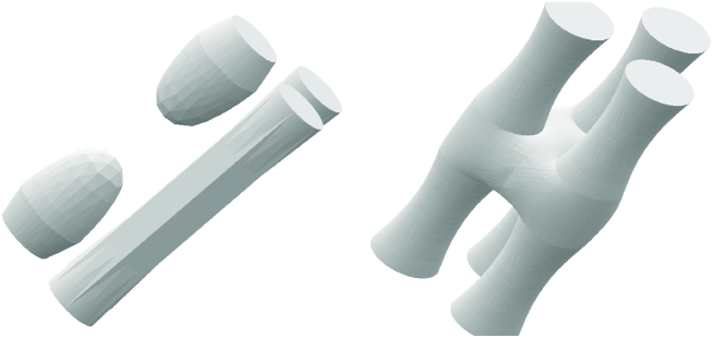
Figure 1: Possible structures for defects in the hexagonal phase : a) - capped cylinders; b) - bridges.

Such experiments have already been performed at the hexagonal-isotropic transition, the loss of hexagonal order upon approaching the transition being monitored by NMR and optical birefringence methods [15, 16]. These experiments have shown that a significant fraction of the surfactant molecules form defects near the isotropic liquid, which can be column ends (with spherical caps) or bridges connecting neighbouring columns (fig.1). It is clear that the nature of the isotropic liquid will be different depending on the nature of the defects. Indeed, column ends will give rise to isolated micelles whereas bridges should rather announce an isotropic liquid formed of cylinders highly connected to each other and randomly oriented.

In order to discriminate between the two possibilities, we measured the diffusion coefficients of a hydrophobic probe (tracer molecule) which is dissolved in the lyotropic mixture (sections 2.1 and 3.1). Indeed, it is reasonable to assume (as demonstrated by the experimental results below) that the tracer is confined to the surfactant cylinders and spends very little time in water. Hence, its diffusion must give valuable structural information about the surfactant aggregates, as we have shown in a recent investigation of the lamellar phase in the C₁₂EO₆/H₂O system [17]. Two transitions were investigated : the $H_{\alpha}\!\rightarrow\!I$ at the azeotropic point of the hexagonal phase (50.0 % C₁₂EO${}_{6}\,$weight concentration) and the $V_{1}\!\rightarrow\!I$ (concentration 59.0 %). The reason why we chose the azeotropic point for the first transition is that the mixture behaves like a pure compound at this particular concentration, i.e. the freezing range vanishes, which allows us to approach the transition very closely [15].

We also measured very precisely the lattice parameter of the hexagonal phase by X-ray scattering and obtained additional qualitative information from the X-ray scattering of the isotropic phase as a function of temperature (sections 2.2 and 3.2). Results are discussed in section 4 within a numerical model for the diffusion of the probe molecules which takes into account the lifetime of the defects. Conclusions are drawn in section 5.

2 Experimental

2.1 Diffusion

The surfactant was purchased from Nikko Ltd. and used without further purification. We used ultrapure water from Fluka. The mixture was carefully homogenized. The samples were prepared between two parallel glass plates, with a spacing of 75 $\mu$m as described in detail elsewhere [15]. The hexagonal phase was then oriented by the directional solidification technique presented in reference [18]. No orientation procedure was needed for the cubic phase, the diffusion tensor being isotropic.

We used a hydrophobic fluorescent dye (NBD-dioctylamin) at a concentration of about $0.1$ w %. Its presence decreases by $\sim 1{\,}^{o}\mbox{C}$ the transition temperature $T_{h}$ at the azeotropic point of the hexagonal phase , but the freezing range remains negligible (about 0.1 ${\,}^{o}\mbox{C}$).

Our method of measuring the diffusion constant is a variant of the technique known as fluorescence recovery after photobleaching (FRAP). The experimental setup was originally designed for the study of thin liquid films [19]. We focused the TEM₀₀ mode of a multimode Ar⁺-ion laser (total power 70 mW) on the sample, bleaching a spot about 40 $\mu$m in diameter. The intensity profile of the beam was approximately Gaussian. Typical bleaching times were of the order of 5 seconds. About $0.5{\,}^{o}\mbox{C}$ below the transition temperature the power had to be decreased to around 15 mW to avoid local melting of the sample. The evolution of the fluorescence intensity profile (proportional to the concentration of non-bleached molecules $c_{\rm n}(x,y,t)$ ) was then monitored for one minute using a cooled CCD camera (Hamamatsu C4742). It is however easier to write the equations for the concentration of bleached molecules, $c(x,y,t)=c_{\rm tot}-c_{\rm n}(x,y,t)$. We write the diffusion equation for the hexagonal phase, with $D_{\|}$ and $D_{\bot}$ the diffusion constants along and across the columns, respectively. In the equation for the cubic or isotropic phase, $D_{\|}$ and $D_{\bot}$ both take the same value, $D_{C}$ or $D_{I}$ respectively. The bleaching is considered uniform through the sample, so the concentration obeys a two-dimensional diffusion equation (in the plane of the sample); the $x$ axis is along the columns : ${\mathbf{e}}_{x}\,\|\,\mathbf{n}$.

$$\frac{\partial c}{\partial t}=D_{\|}\frac{\partial^{2}c}{\partial x^{2}}+D_{\bot}\frac{\partial^{2}c}{\partial y^{2}}+\beta I_{0}c_{\rm n}$$ (1)

where the source term $\beta I_{0}c_{\rm n}$ accounts for the bleaching due to the observation light, of homogenous intensity $I_{0}$; its effect is negligible so we will ignore it from now on.

The initial concentration profile is :

$$c(x,y,0)=\frac{C}{a_{1}a_{2}}\exp\left(-\frac{x^{2}}{{a_{1}}^{2}}-\frac{y^{2}}{{a_{2}}^{2}}\right)$$ (2)

where $a_{1}$ and $a_{2}$ are the semi-axes of the initial spot. The time dependence reads :

$$c(x,y,t)=C\frac{\exp\left(-\frac{x^{2}}{{a_{1}}^{2}+4D_{\|}t}-\frac{y^{2}}{{a_{2}}^{2}+4D_{\bot}t}\right)}{\sqrt{({a_{1}}^{2}+4D_{\|}t)({a_{2}}^{2}+4D_{\bot}t)}}$$ (3)

In the hexagonal phase, where the diffusion is anisotropic, the concentration profile is elliptical. The diffusion coefficients are deduced from the images by fitting a Gaussian function whose adjustable parameters are the two coordinates of the center, the amplitude $C$, the two semi-axes and the angle between the major axis of the ellipse and a given axis in the plane.

2.2 X-Ray Scattering

High resolution X-ray scattering experiments were performed at the H10 experimental station at the LURE synchrotron radiation facility in Orsay, France [20]. A wavelength $\lambda=0.155$ nm was selected by a two crystals monochromator. Harmonic rejection was obtained by reflection of the X-ray beam on two Rh-covered mirrors. The beam size was $0.5\times 2\,\mbox{mm}^{2}$. The sample was set at the center of a Huber diffractometer equipped with a crystal analyzer (Ge 111) . The scattered X-rays were detected with a Bicron point-detector after reflection on the crystal analyzer. The resolution of the diffractometer for a $2\theta$ – scan was 0.002 ^o for the value of $2\theta$ and the FWHM of the direct beam was equal to 0.005 ^o in $2\theta$. For temperature regulation we used a home-made oven and a computer-driven temperature controller.

Samples were contained in flat glass capillaries of thickness 0.1 mm (Vitro Com Inc., Mountain Lakes, New Jersey, U.S.A.). Capillaries were filled with the hexagonal phase at room temperature by suction using a vacuum pump, as described in detail in reference [21]. This procedure allows us to obtain very well aligned samples, the surfactant cylinders being oriented along the capillary long axis by the flow.

In order to investigate the structure of the isotropic phase, X-ray scattering experiments were also performed at the Laboratoire de Physique des Solides using a rotating anode set-up (Cu $K_{\alpha}$, $\lambda$ = 0.154 nm). The X-ray beam delivered by the anode is punctually focused by two perpendicular curved mirrors coated with a 60 nm nickel layer [21]. The mirrors cut the high energy radiation issued from the anode and a 20 $\mu$m nickel foil filters the $K_{\beta}$ emission line. The beam size on the sample was $0.5\times 0.5\,\mbox{mm}^{2}$. The X-ray intensity at the sample level is about $10^{7}$ photons/s mm². The scattered X-rays were detected on imaging plates and the sample – detection distance was 30 cm. Exposure times were typically 10 hours in the liquid isotropic phase.

3 Results

3.1 Diffusion

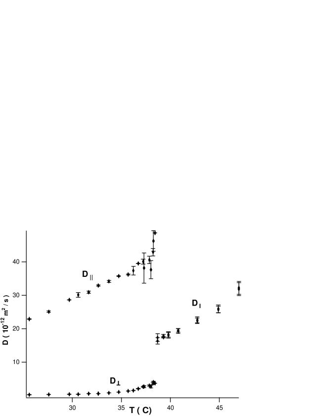
Figure 2: Diffusion coefficients in the hexagonal and isotropic phases : $D_{\|}$, $D_{\bot}$ and $D_{I}$.

The results for the hexagonal-isotropic transition are presented in figures 2 and 3. Far below the transition, both $D_{\|}$ and $D_{\bot}$ in the hexagonal phase follow Arrhenius laws, with activation energies of 0.35 eV and 0.75 eV respectively. Starting at $T\sim T_{h}-5{\,}^{o}\mbox{C}$, the behaviour of $D_{\bot}$ changes. Its value increases rapidly, departing from the activation law and reaches $4.1\,10^{-12}\mbox{ m}^{2}/\mbox{s}$ at the transition temperature $T_{h}=38.60{\,}^{o}\mbox{C}$. The behaviour of $D_{I}$ (in the isotropic phase) also fits with an Arrhenius law, giving an activation energy of 0.65 eV.

Close to the liquid crystal transition temperature we attribute the increase in $D_{\bot}$ to the proliferation of defects connecting the cylinders and providing passage for the tracer molecules. The next section presents a detailed and quantitative discussion of this phenomenon.

In order to confirm this conclusion we measured the diffusion coefficient at the cubic-isotropic phase transition. This type of experiment has already been performed by Monduzzi and coworkers [22] for the self-diffusion coefficient of surfactant in the ionic system CPyCl/NaSal/D₂O. Using PFG-NMR, they found little or no difference between the diffusion coefficients in the cubic and isotropic phases.

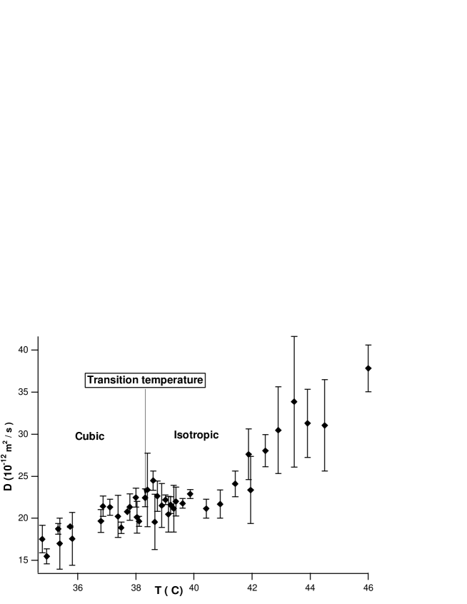
Figure 4: Diffusion coefficients in the cubic and isotropic phases, $D_{C}$ and $D_{I}$. Error bars are obtained by an average over three different measures.

Figure 4 shows our experimental results. The transition temperature is $T_{c}=38.3{\,}^{o}\mbox{C}$. Within experimental accuracy, no discontinuity was observed at the transition. Since the diffusion rate is closely related to the local structure of the phase, we can then conclude that, at least at concentrations of about 60 %, the connectivity of the isotropic phase is similar to that of the bicontinuous cubic one.

3.2 X-Ray Scattering

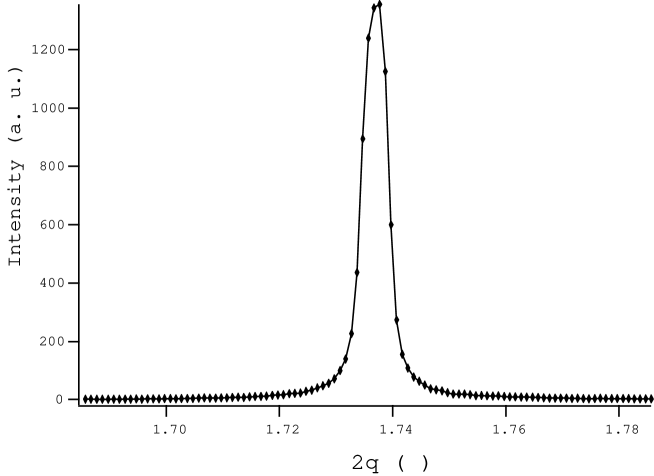
Figure 5: Profile of the (10) Bragg peak in the hexagonal phase (limited by the experimental resolution).

A well oriented sample of the hexagonal phase (50 w% of surfactant) contained in a flat glass capillary of thickness 100 $\mu$m was mounted with a (10) hexagonal Bragg peak in reflection condition [21]. We performed $2\theta$–scans of this peak at different temperatures. One such scan is shown in figure 5. The value of the hexagonal lattice parameter $a$ at a given temperature is obtained from the position $2\theta_{\rm max}$ of the maximum of the diffraction peak :

$$a=\frac{2}{\sqrt{3}}\,d_{\rm 10}=\frac{2}{\sqrt{3}}\,\frac{\lambda}{2\sin(\theta_{\rm max})}=\frac{\lambda}{\sqrt{3}\sin(\theta_{\rm max})}$$ (4)

Thanks to the high resolution of the diffractometer, we were able to detect very small changes (down to 0.002 ^o) of the value of $2\theta_{\rm max}$ versus temperature. The results are plotted in figure 6. Far below the transition to the isotropic liquid phase, $a$ increases linearly with temperature :

$$a=a_{\rm lin}(T)=(5.9-0.0019(T_{h}-T)){\rm nm}$$ (5)

The value of the thermal expansion coefficient is $\displaystyle\frac{1}{a}\frac{{\rm d}a}{{\rm d}T}=3.2\,10^{-4}{\rm K}^{-1}$. Its positive sign accounts for the observation of the zig-zag structure on cooling the hexagonal phase [23]. Near the phase transition, one observes (figure 6) a deviation from the linear temperature dependence, with an additional increase in $a$, $\Delta a=a-a_{\rm lin}$. This effect is observed in the range $(T_{h}-T)<5{\,}^{o}\mbox{C}$, in good agreement with birefringence and NMR observations [15] and the diffusion results.

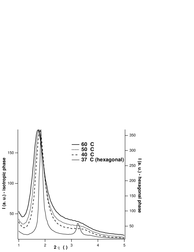
Figure 9: X-ray spectrum in the isotropic phase. A scattering profile in the hexagonal phase is shown for comparison (note the difference in signal intensity).

We performed X-ray scattering measurements on the isotropic phase at the same surfactant concentration (figure 9). For comparison, we also plotted the first two Bragg peaks of the hexagonal phase. It is possible to notice that there is practically no shift of the maximum scattering vector $q_{0}$ upon crossing the transition temperature (compare the curves for 37 ${\,}^{o}\mbox{C}$ and 40 ${\,}^{o}\mbox{C}$). This indicates that there is little change in the local structure of the system. Moreover, the fact that the peak in the isotropic phase is narrow and that a wide shoulder is detectable (corresponding to the second Bragg peak, in position $\sqrt{3}$ as compared to the first), suggests that local order is preserved, up to a distance $d$ that can be estimated as :

$$d\sim a\frac{q_{0}}{\Delta q}\sim 4a$$ (6)

where $\Delta q$ is the width of the peak (in the isotropic phase) from which we subtract the experimental resolution, taken as roughly equal to the width of the Bragg peak in the hexagonal phase [24]. The positional order is maintained up to fourth-neighbours. This should not surprise us, since we are investigating a very concentrated system.

4 Discussion

In this section, we try to relate the pretransitional evolution of $D_{\bot}$ to the appearance of structural defects. Indeed, NMR and birefringence data [15] show that, in the same temperature range ($T_{h}-5{\,}^{o}\mbox{C}$ up to $T_{h}$), the hexagonal order weakens when approaching the transition. This feature can be explained by considering that an increasing fraction of surfactant molecules belongs to the defects. These defects may consist either in a fragmentation of the columns, which become spherically capped cylinders, or in bridges connecting neighboring columns ( figure 1), as discussed in the Introduction (see also reference [15]). A possible structure for the latter type of defects has been proposed in terms of Karcher surfaces connecting columns three by three [25, 26].

4.1 Diffusion

It is clear that connections between cylinders can provide a passage for the tracer molecules, thus leading to the observed increase in $D_{\bot}$. The presence of defects of the first type (capped cylinders) can be ruled out, since it would bring about a decrease in $D_{\|}$, which does not appear in our measurements. We will assume in the following that the only defects present are of the ‘bridge’ type (figure 1 – b). This conclusion is coherent with the fact that the curvature of the aggregates diminishes with increasing temperature (due to the decreasing hydration of the nonionic polar groups [27, 28]) which clearly favours the merging of the cylinders over their breaking up.

Let us now estimate the density of defects $n_{\rm def}$ (number of defects per unit volume). In order to do so, we must quantify their role in transverse diffusion by relating $n_{\rm def}$ to $D_{\rm def}=D_{\bot}-D_{\rm norm}$ (where $D_{\rm norm}$ is the “normal” behaviour of $D_{\bot}$, extrapolated from low temperature). We shall denote by $a\simeq 6\mbox{ nm}$ (see figure 6) the parameter of the hexagonal lattice and let $L$ be the average distance between connections along a cylinder. The adimensional parameter $x=a/L$ provides a quantitative measure of the defect density, since $n_{\rm def}=\frac{2}{3\sqrt{3}a^{3}}x$ [29]. We shall see in the following that the diffusion contribution of the defects also depends on their lifetime, $\tau$. Throughout the discussion, we will consider only the type of defects depicted in figure 1 – b, connecting three neighbouring cylinders.

In the case where the lifetime of the defects is very short compared to the characteristic diffusion time of the molecules, $D_{\rm def}$ can be evaluated analytically. The molecule has a constant probability $x$ to encounter a defect. Once a defect is reached, the molecule can either cross it, or continue to move along the cylinder, with equal probability, so that it will spend (on average) $x/2$ of its time crossing defects and $1-x/2$ travelling along the columns. Denoting by $z$ the axis of the cylinders and by $\rho$ the position vector in the plane orthogonal to $z$, the presence probability for a particle starting a random walk at the origin is (time is given in units of $t_{0}$, the elementary step) :

$$P({\mbox{\boldmath{$\rho$}}},z,t)=C(t)\exp\left(\frac{-z^{2}}{2a^{2}(1-x/2)t}\right)\exp\left(\frac{-{\mbox{\boldmath{$\rho$}}}^{2}}{(4/3)a^{2}(x/2)t}\right)$$ (7)

where $C(t)$ is a normalisation factor depending only on the time; the numerical factors 2 and 4/3 are the ones for random walks respectively in 1D and in 2D on a hexagonal network. Keeping in mind that we are interested not in the density along $\rho$, but in its projection on the fixed plane of the sample (which gives an additional factor $1/\sqrt{2}$ ) we can estimate the ratio $\displaystyle r=D_{\rm def}/{D_{\|}}$ as being :

$$r=\frac{2}{3\sqrt{2}}\frac{x/2}{1-x/2}$$ (8)

In order to check the validity of formula (8), and to investigate the influence of the defect lifetime, we have performed Monte Carlo numerical simulations. We generate random walks on a 3D lattice which reproduces the hexagonal structure. The elementary RW jump is equal to the lattice parameter. In the absence of defects, the particle only diffuses along axis $z$. Defects connecting three nearest-neighbour cylinders are introduced in order to allow transverse diffusion. When a defect is encountered, the particle has a probability of 1/2 to remain on the same cylinder and equal probabilities 1/4 to jump on one or the other of the two connected neighbours.

One elementary RW step defines the unit time in the simulation. Defects have a lifetime $\tau$ which means that, every $\tau$ elementary steps, all the defects are erased and replaced again at random.

Each RW has $10^{4}$ steps and the probability distribution is averaged over $10^{4}$ RWs.

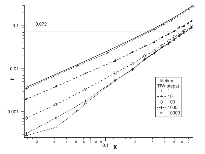
Figure 8: $\displaystyle r=D_{\rm def}/{D_{\|}}$ plotted against $x=a/L$ for different defect lifetimes $\tau$.

The statistics of particle positions gives us the diffusion coefficients both the parallel (along the $z$ axis) and transversal diffusion coefficients. Their ratio $\displaystyle r=D_{\rm def}/{D_{\|}}$ is plotted against $x=a/L$ (figure 8) for different lifetimes $\tau$.

For $\tau=1$, the defect configuration should be changed at every RW step and the simulation would require too much time. However, since the defect positions are completely decorrelated from one step to the other, the solution adopted was to give each particle a constant probability $x$ of encountering a defect. We see that the dependence $r(x)$ is very well described by equation (8) (solid line in figure 8).

It is clear from figure 8 that increasing the stability of the defects lessens their efficiency for tracer diffusion or, in other words, more defects are needed to obtain a given value of $r$ when $\tau$ becomes larger : if for $\tau=1$ a density $x\simeq 0.25$ is needed in order to reach the value measured just before the transition to the isotropic phase $r=D_{\rm def}/D_{\|}=0.072$, for $\tau=10$ one already has $x\simeq 0.5$.

The dependence of $r(x)$ also changes its character with increasing $\tau$ : for $\tau=1$, $r\sim x$ (to leading order), while for frozen-in defects ($\tau=10^{4}$), $r\sim x^{2}$. This is because, in order to jump from a cylinder to the next one at a distance $a$, the molecule has to diffuse along $z$ for a distance $L$ :

$$t_{\rm jump}\sim\frac{a^{2}}{D_{\rm def}}\sim\frac{L^{2}}{{D_{\|}}}\Longrightarrow r=\frac{D_{\rm def}}{{D_{\|}}}\sim\frac{a^{2}}{L^{2}}=x^{2}$$ (9)

Since the defects are at equilibrium, their density $n_{\rm def}$ is given by a Boltzmann factor

$$n_{\rm def}=n_{0}\exp\left(\frac{-E_{\rm def}}{k_{B}T}\right)$$ (10)

where $E_{\rm def}$ is the energy of the defect as compared to the perfectly ordered structure. The fact that the number of defects increases abruptly close to the transition temperature means that their energy decreases (we will neglect the increase in thermal energy : $k_{B}T\simeq k_{B}T_{h}$ in the vicinity of the transition). The simplest assumption is that of a linear behaviour :

$$E_{\rm def}=\alpha(T_{h}-T)+E_{0}$$ (11)

The birefringence and NMR measurements [15] give (by fitting $n_{\rm def}(T)$) a value $\alpha=225\,k_{B}$; our fit for $D_{\rm def}(T)$ (see figure 3) gives $\alpha=180\,k_{B}$. We can thus consider that $D_{\rm def}\sim n_{\rm def}$, which supports our hypothesis that the defects have very short lifetimes. It is then justified to use (8) for evaluating the mean distance between connections at the transition temperature $L_{0}$ : $L_{0}\simeq 4a\simeq 25\,\mbox{nm}$, in fairly good agreement with results of reference [15], which gives $L_{0}\simeq\mbox{17 nm}$. An important consequence is that the density of defects in the hexagonal phase is large at the transition; the picture of the hexagonal phase as being formed of infinitely long parallel columns is no longer accurate in these conditions.

We can thus infer that the isotropic phase above the hexagonal mesophase has a highly connected structure.

4.2 X-ray scattering

The additional increase in lattice parameter $\Delta a$ (figure 6) can also be explained by the appearance of connections close to the transition. In this paragraph, we derive a very simple relation between $\Delta a$ and the fraction $f$ of surfactant molecules involved in the connections.

The X-ray peak provides a measure for the parameter of the hexagonal lattice formed by the surfactant cylinders. If a fraction $f$ of molecules is involved in transversal junctions between cylinders, a fraction $(1-f)$ of molecules are still inside the cylinders. Mass conservation then demands that in a given volume, the total number of cylinders is divided by $1/(1-f)$ and the lattice parameter is multiplied by a factor $\displaystyle\frac{1}{\sqrt{1-f}}$ (because the cylinders form a 2D hexagonal array). The value of $f$ as a function of temperature is given by the relation :

$$a(T)=\frac{a_{\rm lin}(T)}{\sqrt{1-f}}\Longrightarrow f=1-\left[\frac{a_{\rm lin}(T)}{a(T)}\right]^{2}$$ (12)

where the value $a_{\rm lin}(T)$ is extrapolated from the low-temperature behaviour in the region near the transition (solid line in 6). From this relation we obtain $f(T)$, which fits well with an exponential law, as plotted in figure 7.

The fact that we find an exponential law for $f(T)$ for $0<T_{h}-T<5{\,}^{o}\mbox{C}$ is in agreement with the tracer diffusion results and the NMR and birefringence experiments [15]. However, we obtain $f(T_{h})=1.3\%$, much less than the value of $8\%$ estimated in reference [15] (and a value of the parameter $\alpha\simeq 100k_{B}T$, about half of that given by the birefringence experiment). This is not very surprising, since it is reasonable to assume that the connections induce an elastic deformation of the hexagonal lattice, which will also affect the value of the average lattice parameter $a$ as measured by X-ray scattering. If such a contribution tends to reduce locally the value of $a$ (the cylinders getting closer together), then the simple relation (12) underestimates the value of $f$.

5 Conclusion

The investigation of the C₁₂EO₆/H₂O system by means of diffusion coefficients measurements and X-ray scattering allowed us to obtain a clearer image of its isotropic phase for high surfactant concentration (50–60 %). The data was mainly obtained by studying the pretransitional effects that appear in the hexagonal and bicontinuous cubic mesophases close to the transition towards the isotropic phase.

The increase of the diffusion coefficient across the cylinders ($D_{\bot}$) in the hexagonal phase for a hydrophobic fluorescent dye proves that very mobile defects, consisting in connections between the cylinders, appear close to the transition.

This information is corroborated by the anomalous increase of the lattice parameter $a$ in the same temperature range. The X-ray scattering of the isotropic phase shows a well-defined and fairly narrow peak corresponding to the first Bragg peak in hexagonal phase.

No detectable jump in diffusion coefficient occurred at thetransition between the cubic and isotropic phases, showing that the surfactant aggregates in the two phases are very similar.

We can therefore conclude that, in the concentration range that we investigated, the isotropic phase of the C₁₂EO₆/H₂O system is probably composed of very long surfactant cylinders locally preserving the hexagonal order (even though long-range order is lost), forming a highly connected and rapidly fluctuating structure.

Acknowledgements. M. Gailhanou (LURE, beamline H10) is warmly thanked for taking part in the synchrotron X-ray scattering experiments. We acknowledge fruitful discussions with Robert Hołyst. D. C. gratefully acknowledges financial support from the research group ‘Liquid crystals in confined geometries’ during his stay in Orsay.

FIGURES

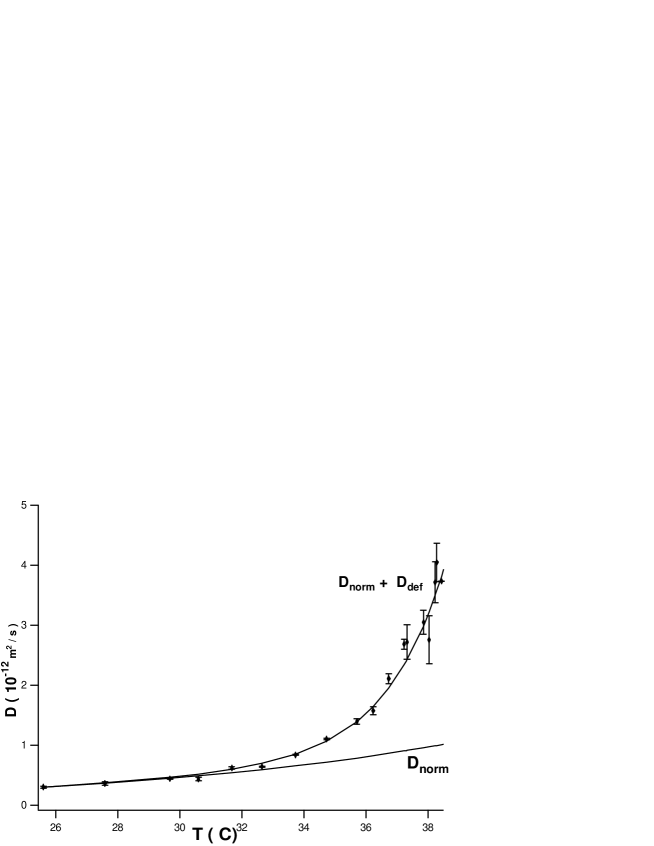
Figure 3: $D_{\bot}$ in the hexagonal phase. Error bars are obtained by an average over three different measures. The straight line represents the extrapolation of low-temperature behaviour. The solid curve is an exponential fit (see text).

Figure 6: Lattice parameter $a$ vs. temperature in the hexagonal phase. The line is the extrapolation of low-temperature behaviour.

Figure 7: The fraction $f$ of molecules present in the defects as a function of temperature. Line is an exponential fit (see text).

References

- [1] Mitchell, D. J. et al., J. Chem. Soc. Faraday Trans. 1, 1983, 79, 975.
- [2] Tolédano, P. and Figueiredo Neto, A. M. (eds.), Phase Transitions in Complex Fluids World Scientific, 1998.
- [3] Nilsson, P. G.; Wennerström, H.; Lindmann, B. J. Phys. Chem., 1983, 87, 1377.
- [4] Brown, W. et al., J. Phys. Chem., 1983, 87, 4549.
- [5] Brown, W.; Rymdén, R. J. Phys. Chem., 1987, 91, 3565.
- [6] Brown, W.; Zhou, P.; Rymdén, R. J. Phys. Chem., 1988, 92, 6086.
- [7] Jonströmer, J.; Jönsson, B.; Lindmann, B. J. Phys. Chem., 1991, 95, 3293.
- [8] Zulauf, M. et al. J. Phys. Chem., 1985, 89, 3411.
- [9] Triolo, R.; Magid, L. J.; Johnson, J. S. Jr.; Child, H. R. J. Phys. Chem., 1982, 86, 3689.
- [10] Magid, L. J.; Triolo, R.; Johnson, J. S. Jr. J. Phys. Chem., 1984, 88, 5730.
- [11] Richtering, W. H.; Burchard, W.; Jahns, E.; Finkelmann, H. J. Phys. Chem., 1988, 92, 6032.
- [12] Cebula, D. J.; Ottenill, R. M. Colloid. Polym. Sci., 1982, 260, 260.
- [13] Ravey, J.-C. J. Colloid. Interface Sci., 1983, 94, 289.
- [14] D’Arrigo, G.; Briganti, G. Phys. Rev. E, 1998, 92, 713.
- [15] Sallen, L.; Sotta, P.; Oswald, P. J. Phys. Chem. B, 1997, 101, 4875.
- [16] L. Sallen, Thesis, Ecole Normale Supérieure de Lyon, France, 1996 (Order No. 23).
- [17] Constantin, D.; Oswald, P. accepted by Phys. Rev. Lett.
- [18] Oswald, P. et al. J. Phys III, 1993, 3, 1891.
- [19] Bechhoefer, J. et al. Phys. Rev. Lett., 1997, 79, 4922.
- [20] Gailhanou, M. et al. submitted to Nuclear Instruments and Methods A.
- [21] Impéror-Clerc, M.; Davidson, P. EPJB, 1999, 9, 93.
- [22] Monduzzi, M.; Olsson, U.; Söderman, O. Langmuir, 1993, 9, 2914.
- [23] The ‘zig-zag’ texture is the result of an undulation instability that develops upon dilating the system (Oswald, P. et al. J. Phys II, 1996, 6, 1).
- [24] In the hexagonal phase, the Bragg peak should be a Dirac function (infinite lattice). Its width is only given by the experimental resolution. We must therefore subtract this width in order to assess the order in the isotropic phase. The remaining gives then a direct measure of local order in the system : if is the distance over which hexagonal order is preserved, , as ; hence, the relation 6.
- [25] Clerc, M.; Levelut, A. M.; Sadoc, J. F. J. Phys. II, 1991, 1, 1263.
- [26] Karcher, H. Manuscr. Math., 1989, 64, 291.
-
[27]
Israelachvili, J. N. Intermolecular and Surface Forces, 2nd ed.;
Academic Press: London, 1992. - [28] Puvvada, S.; Blanckstein, D. J. J. Chem. Phys., 1990, 92, 3710.
- [29] To obtain this formula, one can use the fact that each defect connects three cylinders, so the number of individual connections is three times the number of defects, i. e. in a volume there are connections; in the same volume, the total cylinder length is given by , since is the size of the elementary cell in the hexagonal phase. The mean distance between connections is therefore .