Measurements of ${\bm{\psi(3686)\rightarrow K^{-}\Lambda\bar{\Xi}^{+}}+c.c.}$ and ${\bm{\psi(3686)\rightarrow\gamma K^{-}\Lambda\bar{\Xi}^{+}}+c.c.}$

Abstract

Using a sample of $1.06\times 10^{8}\ \psi(3686)$ events produced in $e^{+}e^{-}$ collisions at $\sqrt{s}$ = 3.686 GeV and collected with the BESIII detector at the BEPCII collider, we present studies of the decays $\psi(3686)\rightarrow K^{-}\Lambda\bar{\Xi}^{+}+c.c.$ and $\psi(3686)\rightarrow\gamma K^{-}\Lambda\bar{\Xi}^{+}+c.c.$. We observe two hyperons, $\Xi(1690)^{-}$ and $\Xi(1820)^{-}$, in the $K^{-}\Lambda$ invariant mass distribution in the decay $\psi(3686)\rightarrow K^{-}\Lambda\bar{\Xi}^{+}+c.c.$ with significances of $4.9\sigma$ and $6.2\sigma$, respectively. The branching fractions of $\psi(3686)\rightarrow K^{-}\Lambda\bar{\Xi}^{+}+c.c.$, $\psi(3686)\rightarrow K^{-}\Sigma^{0}\bar{\Xi}^{+}+c.c.$, $\psi(3686)\to\gamma\chi_{cJ}\to\gamma K^{-}\Lambda\bar{\Xi}^{+}+c.c.$ $(J=0,\ 1,\ 2)$, and $\psi(3686)\to\Xi(1690/1820)^{-}\bar{\Xi}^{+}+c.c$ with subsequent decay $\Xi(1690/1820)^{-}\to K^{-}\Lambda$ are measured for the first time.

I INTRODUCTION

The quark model, an outstanding achievement of the last century, provides a rather good description of the hadron spectrum. However, baryon spectroscopy is far from complete, since many of the states expected in the SU(3) multiplets are either undiscovered or not well established quarkmodel , especially in the case of cascade hyperons with strangeness $S=-2$, the $\Xi^{*}$. Due to the small production cross sections and the complicated topology of the final states, only eleven $\Xi^{*}$ states have been observed to date. Few of them are well established with spin-parity determined, and most observations and measurements to date are from bubble chamber experiments or diffractive $K^{-}p$ interactions pdg .

As shown by the Particle Data Group (PDG), most $\Xi^{*}$ hyperon results obtained to date have limited statistics pdg . For example, the $\Xi(1690)^{-}$ was first observed in the $\Sigma\bar{K}$ final state in the reaction $K^{-}p\to(\Sigma\bar{K})K\pi$ x6 . Afterwards its existence has been confirmed by other experiments biagi ; x6wa89 ; x6belle , but its spin-parity was not well determined. More recently, BABAR reported evidence for $J^{P}=1/2^{-}$ for the $\Xi(1690)$ by analyzing the Legendre Polynomial moments of the $\Xi^{-}\pi^{+}$ system in the decay $\Lambda_{c}^{+}\to\Xi^{-}\pi^{+}K^{+}$ x6babar . Clear evidence for $\Xi(1820)$ was observed in the $K^{-}\Lambda$ mass spectrum from a sample of 130$\pm$16 events in $K^{-}p$ interactions gay , and the $J=1/2$ assumption was ruled out by using the Byers and Fenster technique byers . Ten years later, a CERN-SPS experiment indicated that $\Xi(1820)$ favors negative parity in the case of $J=3/2$ biagi2 .

At present, the $\Xi(1690)$ and $\Xi(1820)$ are firmly established. Further investigation of their properties, e.g. mass, width and spin-parity, is important to the understanding of $\Xi^{*}$ states. Besides scattering experiments, decays from charmonium states offer a good opportunity to search for additional $\Xi^{*}$ states. Although charmonium decays into pairs of $\Xi^{(*)}$ states are suppressed by the limited phase space, the narrow charmonium width which reduces the overlap with the neighboring states and the low background allow the investigation of these hyperons with high statistics charmonium samples.

Furthermore, our knowledge of charmonium decays into hadrons, especially to hyperons, is limited. The precise measurements of the branching fractions of charmonium decays may help provide a better understanding of the decay mechanism. The large $\psi(3686)$ data sample collected with the BESIII detector provides a good opportunity to study the cascade hyperons.

In this paper, we report on a study of the decays $\psi(3686)\rightarrow K^{-}\Lambda\bar{\Xi}^{+}+c.c.$ and $\psi(3686)\rightarrow\gamma K^{-}\Lambda\bar{\Xi}^{+}+c.c.$ based on a sample of 1.06$\times 10^{8}$ $\psi(3686)$ events psipNo collected with the BESIII detector. Another data sample, consisting of an integrated luminosity of $44.5\;\text{pb}^{-1}$ lumi taken below the $\psi(3686)$ peak at $\sqrt{s}=3.65\;\text{GeV}$, is used to estimate continuum background. Evidence for the $\Xi(1690)^{-}$ and $\Xi(1820)^{-}$ is observed in the $K^{-}\Lambda$ invariant mass distribution in the decay $\psi(3686)\rightarrow K^{-}\Lambda\bar{\Xi}^{+}+c.c.$ In the following, the charge conjugate decay mode is always implied unless otherwise specified.

II DETECTOR AND MONTE CARLO SIMULATION

BEPCII is a two-ring collider designed for a luminosity of $10^{33}$ cm^-2s^-1 at the $\psi(3770)$ resonance with a beam current of $0.93\;\text{A}$. The BESIII detector has a geometrical acceptance of 93% of $4\pi$, and consists of a helium-gas-based drift chamber (MDC), a plastic scintillator time-of-flight system (TOF), a CsI(Tl) electromagnetic calorimeter (EMC), a superconducting solenoid magnet providing 1.0 T magnetic field, and a resistive plate chamber-based muon chamber (MUC). The momentum resolution of charged particles at 1 GeV/$c$ is 0.5%. The time resolution of the TOF is 80 ps in the barrel detector and 110 ps in the end cap detectors. The photon energy resolution at 1 GeV is 2.5% (5%) in the barrel (end caps) of the EMC. The trigger system is designed to accommodate data taking at high luminosity. A comprehensive description of the BEPCII collider and the BESIII detector is given in Ref. bes .

A GEANT4-based geant4 MC simulation software BOOST boost , which includes geometric and material description of the BESIII detector, detector response and digitization models as well as tracking of the detector running condition and performance, is used to generate MC samples. A series of exclusive MC samples, $\psi(3686)\to\gamma\chi_{cJ}\to\gamma K^{-}\Lambda\Xi^{+}$, $\psi(3686)\rightarrow K^{-}\Lambda\bar{\Xi}^{+}$, $\psi(3686)\rightarrow K^{-}\Sigma^{0}\bar{\Xi}^{+}$ are generated to optimize the selection criteria and estimate the corresponding selection efficiencies. The production of $\psi(3686)$ is simulated by the generator KKMC kkmc1 ; kkmc2 . The decay $\psi(3686)\to\gamma\chi_{cJ}$ is assumed to be a pure $E1$ transition and to follow a $1+\alpha\cos^{2}\theta$ angular distribution with $\alpha=1,-1/3$ and $1/13$ for $J$ = 0, 1 and 2, respectively e1 , where $\theta$ is the polar angle of the photon. The other subsequent decays are generated with BesEvtGen besevtgen1 with a uniform distribution in phase space. An inclusive MC sample, consisting of $1.06\times 10^{8}$ $\psi(3686)$ events, is used to study potential backgrounds, where the known decay modes of $\psi(3686)$ are generated by BesEvtGen with branching fractions at world average values pdg , and the remaining unknown decay modes are modeled by LUNDCHARM lundc .

III ANALYSIS OF $\bm{\psi(3686)\rightarrow K^{-}\Lambda\bar{\Xi}^{+}}$

The decay $\psi(3686)\rightarrow K^{-}\Lambda\bar{\Xi}^{+}$ is reconstructed from the cascade decays $\Lambda\to p\pi^{-}$, $\bar{\Xi}^{+}\to\bar{\Lambda}\pi^{+}$ and $\bar{\Lambda}\to\bar{p}\pi^{+}$. At least six charged tracks are required and their polar angles $\theta$ must satisfy $|\cos\theta|<0.93$. The combined TOF and $dE/dx$ information is used to form particle identification (PID) confidence levels for pion, kaon and proton hypotheses. Each track is assigned to the particle hypothesis type with the highest confidence level. Candidate events are required to have one kaon. If more than one kaon candidate is identified, only the kaon with highest confidence level is kept, and the others are assumed to be pions. The same treatment is implemented for the proton and antiproton. The final identified charged kaon is further required to originate from the interaction point (IP), i.e., the point of its closest approach to the beam is within 1 cm in the plane perpendicular to beam and within $\pm 10\;\text{cm}$ along the beam direction.

In the analysis, constraints on the secondary decay vertices of the long lived particles, $\Lambda$ and $\bar{\Xi}^{+}$, are utilized to suppress backgrounds. $\Lambda$ particles are reconstructed using secondary vertex fits on $p\pi^{-}$ pairs. For events with more than one $\Lambda$ candidate, the one with the smallest $\chi^{2}$ for the secondary vertex fit is selected. $\bar{\Xi}^{+}$ candidates are reconstructed in two steps. A $\bar{p}\pi^{+}$ pair sharing a common vertex is selected to reconstruct the $\bar{\Lambda}$ candidate, and the common vertex is regarded as its decay vertex. The $\bar{\Xi}^{+}$ is then reconstructed with a $\bar{\Lambda}$ candidate and another $\pi^{+}$ by implementing another secondary vertex fit. For events with more than one $\bar{\Xi}^{+}$ candidate, the $\bar{p}\pi^{+}\pi^{+}$ combination with the minimum $|M(\bar{p}\pi^{+})-M(\bar{\Lambda})|$ is selected, where $M(\bar{p}\pi^{+})$ is the invariant mass of the $\bar{\Lambda}$ candidate from the secondary vertex fit, and $M(\bar{\Lambda})$ is the corresponding nominal mass from the PDG pdg .

\begin{overpic}[width=390.25534pt]{plots/df_m_2d_log.eps} \put(13.0,63.0){{\bf(a)}} \put(63.0,63.0){{\bf(b)}} \put(13.0,28.0){{\bf(c)}} \put(63.0,28.0){{\bf(d)}} \end{overpic}

Figure 1: Invariant mass distribution of (a) $p\pi^{-}$ and (b) $\bar{p}\pi^{+}$ (with the $\Lambda$ mass window requirement). The arrows indicate the mass windows used in the analysis (see text). (c) Scatter plot of $M(p\pi^{-})$ versus $M(\bar{\Lambda}\pi^{+})$ for data. (d) $\bar{\Lambda}\pi^{+}$ invariant mass distribution. In the one dimensional plots, the points with error bars are the data, the solid histograms are MC distributions normalized to the data, and the shaded histogram is the background estimated from the inclusive MC sample. The solid and long-dashed lines represent the fit curve and the background contribution from the fit.

The selected $K^{-}$, $\Lambda$, and $\bar{\Xi}^{+}$ candidates are subjected to a four-momentum constraint kinematic fit (4C-fit) under the hypothesis of $\psi(3686)\rightarrow K^{-}\Lambda\bar{\Xi}^{+}$, and $\chi^{2}_{4C}<200$ is required to further suppress the potential backgrounds and to improve the resolution. Figure 1 (a) shows the invariant mass distribution of $p\pi^{-}$, $M(p\pi^{-})$, where a $\Lambda$ peak is clearly visible. A mass window requirement $1.110<M(p\pi^{-})<1.121$ GeV/$c^{2}$, corresponding to 6 times the mass resolution, is imposed to select $\Lambda$ candidates. With the above selection criteria, the invariant mass of the $\bar{\Lambda}$ candidate $M(\bar{p}\pi^{+})$ is shown in Fig. 1 (b), and a clean $\bar{\Lambda}$ peak is observed. A mass window requirement $1.110<M(\bar{p}\pi^{+})<1.121$ GeV/$c^{2}$ is applied to further improve the purity. Figure 1 (c) shows the scatter plot of $M(p\pi^{-})$ versus $M(\bar{\Lambda}\pi^{+})$ without the $\Lambda$ mass window requirement, where the accumulated events around the $\Lambda$-$\Xi$ mass region are from the decay $\psi(3686)\rightarrow K^{-}\Lambda\bar{\Xi}^{+}$. The projection of $M(\bar{\Lambda}\pi^{+})$ for all surviving events is shown in Fig. 1 (d), where the $\bar{\Xi}^{+}$ peak is seen with very low background.

Potential non-$\bar{\Xi}^{+}$ backgrounds are studied with the $\psi(3686)$ inclusive MC sample by imposing the same selection criteria. The corresponding distribution of $M(\bar{\Lambda}\pi^{+})$ is shown in Fig. 1 (d) as the shaded histogram. The background is well described by the inclusive MC sample and is flat. Backgrounds are also investigated with the $M(p\pi^{-})$ versus $M(\bar{p}\pi^{+})$ 2-dimensional sideband events from the data sample, where the sideband regions are defined as $1.102<M(p\pi^{-}/\bar{p}\pi^{+})<1.107$ GeV/$c^{2}$ and $1.124<M(p\pi^{-}/\bar{p}\pi^{+})<1.130$ GeV/$c^{2}$. No peaking structure is observed in the $M(\bar{\Lambda}\pi^{+})$ distribution around the $\bar{\Xi}^{+}$ region. To estimate the non-resonant background coming directly from $e^{+}e^{-}$ annihilation, the same selection criteria are implemented on the data sample taken at $\sqrt{s}$ = 3.65 GeV. Only 1 event with $M(\bar{\Lambda}\pi^{+})$ at 1.98 GeV/$c^{2}$, located outside of the $\bar{\Xi}^{+}$ signal region, survives, which is normalized to an expectation of 3.6 events in $\psi(3686)$ data after considering the integrated luminosities and an assumed $1/s$ dependence of the cross section, as $L(\sqrt{s})\propto N_{\text{obs}}/\sigma_{\text{QED}}(\sqrt{s})$ psipNo , where $L$ is the integrated luminosity and $\sigma_{\text{QED}}$ is the cross section of QED processes. Therefore, the non-resonant background can be neglected.

III.1 BRANCHING FRACTION MEASUREMENT

To determine the event yield, an extended unbinned maximum likelihood fit is performed on the $M(\bar{\Lambda}\pi^{+})$ distribution in Fig. 1 (d). In the fit, the $\bar{\Xi}^{+}$ is described by a double Gaussian function, and the background is parameterized by a first order Chebychev polynomial function. The fit result, shown as the solid curve in Fig. 1 (d), yields $N_{\text{obs}}=236.4\pm 16.6$ $\bar{\Xi}^{+}$ candidates. The decay branching fraction $\mathcal{B}({\psi(3686)\rightarrow K^{-}\Lambda\bar{\Xi}^{+}})$ is calculated to be

$$\mathcal{B}(\psi(3686)\rightarrow K^{-}\Lambda\bar{\Xi}^{+}){}$$

$$=\frac{N_{\text{obs}}}{N_{\psi(3686)}\cdot\mathcal{B}^{2}(\Lambda\to p\pi^{-})\cdot\mathcal{B}(\Xi^{-}\to\Lambda\pi^{-})\cdot\epsilon}{}$$

$$=(3.86\pm 0.27)\times 10^{-5},$$ (1)

where $N_{\psi(3686)}=(106.41\pm 0.86)\times 10^{6}$ is the number of $\psi(3686)$ events determined with inclusive hadronic events psipNo , $\epsilon=14.1\%$ is the detection efficiency, evaluated from the MC sample simulated with a uniform distribution in phase-space, and $\mathcal{B}(\Lambda\rightarrow p\pi^{-})$ and $\mathcal{B}(\bar{\Xi}^{+}\rightarrow\bar{\Lambda}\pi^{+})$ are the corresponding decay branching fractions pdg . The uncertainty is statistical only.

III.2 OBSERVATION OF $\bm{\Xi}^{*-}$ STATES

In the distribution of the $K^{-}\Lambda$ invariant mass, $M(K^{-}\Lambda)$, structures around 1690 and 1820 MeV/$c^{2}$, assumed to be $\Xi(1690)^{-}$ and $\Xi(1820)^{-}$, are evident with rather limited statistics. In order to improve the statistics, a partial reconstruction method is used where the $K^{-}$ and $\Lambda$ are required but the reconstruction of $\bar{\Xi}^{+}$ and the 4C kinematic fit are omitted. In addition, an identified anti-proton is required among the remaining charged tracks to suppress background. With the above loose selection criteria, the distribution of $M(p\pi^{-})$ is shown in Fig. 2 (a), where a $\Lambda$ is observed. After applying the $M(p\pi^{-})$ mass window requirement, $1.110<M(p\pi^{-})<1.121$ GeV/$c^{2}$, the distribution of the mass recoiling against the $K^{-}\Lambda$ system $RM(K^{-}\Lambda)$ is shown in Fig. 2 (b), where the $\bar{\Xi}^{+}$ is observed, although with a higher background than in the full reconstruction. With a requirement of $1.290<RM(K^{-}\Lambda)<1.345$ GeV/$c^{2}$, the $\Xi(1690)^{-}$ and $\Xi(1820)^{-}$ are observed in the $M(K^{-}\Lambda)$ distribution with improved statistics, as shown in Fig. 3. MC studies show that the event selection efficiency is improved by a factor of two using the partial reconstruction method.

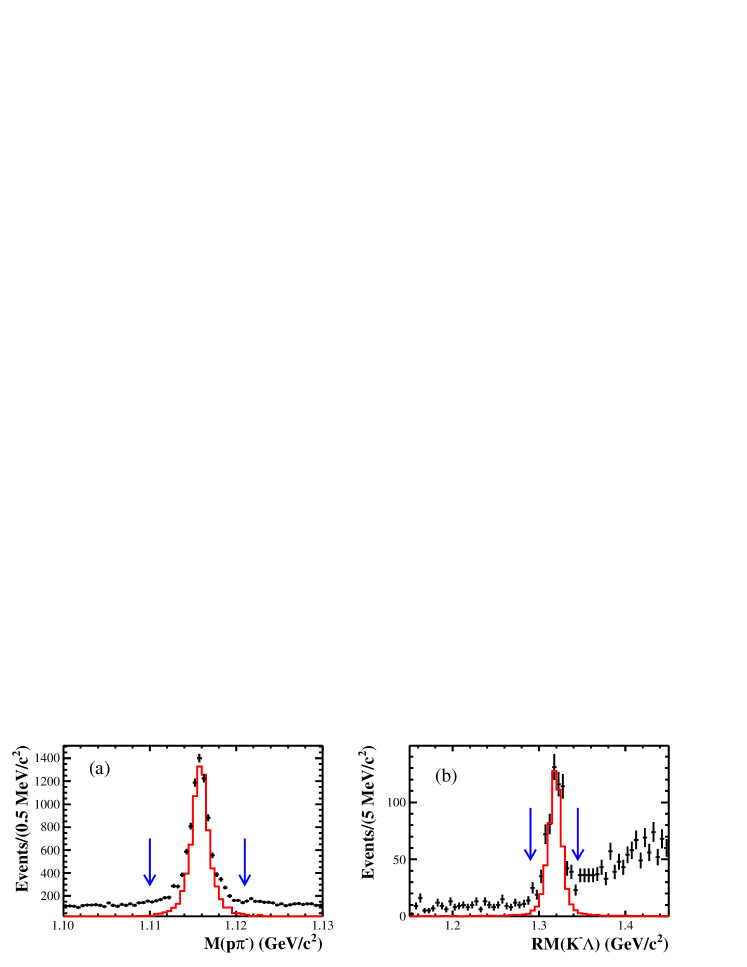
Figure 2: Invariant mass spectrum (a) of $p\pi^{-}$, and (b) of the mass recoiling against the $K^{-}\Lambda$ system. The dots with error bars show the distribution for data, and the solid histogram shows that for the exclusive MC normalized to the data in the signal region. The arrows indicate the selection region used in the analysis (see text).

To ensure that the observed structures are not from background, potential backgrounds are investigated using both data and inclusive MC samples. Non-$\Lambda$ ($\bar{\Xi}^{+}$) background is estimated from the events in the $\Lambda$ ($\bar{\Xi}^{+}$) sideband regions, defined as $1.102<M(p\pi^{-})<1.107$ GeV/$c^{2}$ and $1.124<M(p\pi^{-})<1.130$ GeV/$c^{2}$ ($1.243<RM(K^{-}\Lambda)<1.270$ GeV/$c^{2}$ and $1.365<RM(K^{-}\Lambda)<1.393$ GeV/$c^{2}$), and their $M(K^{-}\Lambda)$ distribution is shown in Fig. 3 with the dot-dashed (dashed) histogram. Possible background sources are also investigated with the inclusive MC sample, and the result is shown with the shaded histogram in Fig. 3. No evidence of peaking structures in the $M(K^{-}\Lambda)$ distribution is observed in either the sideband region or the inclusive MC sample. The same selection criteria are applied to the data sample collected at 3.65 GeV to estimate the background coming directly from $e^{+}e^{-}$ annihilation. Only one event with $M(K^{-}\Lambda)$ around 1.98GeV survives, which corresponds to an expected 3.6 events when normalized to the $\psi(3686)$ sample. This background can therefore be neglected.

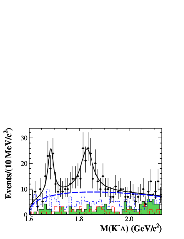
Figure 3: Invariant $K^{-}\Lambda$ mass distribution. Points with error bars represent data, and the solid and dashed curves are the fit curve and the non-resonant contribution obtained from the fit. The shaded histogram represents the background estimated from the inclusive MC sample, and the dashed and dot-dashed histograms are the $\Lambda$ sideband and the $\bar{\Xi}^{+}$ sideband backgrounds from data, respectively.

An extended unbinned maximum likelihood fit of the $M(K^{-}\Lambda)$ distribution is performed to determine the resonance parameters and event yields of the excited $\Xi^{*-}$ hyperons. In the fit, the $\Xi^{*-}$ shapes are described by Breit-Wigner functions $A_{i}(m)$ convoluted with Gaussian functions $G(m,\mu,\sigma)$, which represent the mass shift and resolution in the reconstruction, multiplied by the mass dependent efficiency $\varepsilon(m)$, $\varepsilon(m)[G(m,\mu_{i},\sigma_{i})\otimes A^{2}_{i}(m)]$. In the fit, both parameters of $G(m,\mu,\sigma)$ and $\varepsilon(m)$ are fixed the the values determined from the studies to exclusive MC samples, and the Breit-Wigner function $A_{i}(m)$ is described below. The shape of background is parameterized by a function $B(m)=(m-m_{0})^{1/2}+c(m-m_{0})^{3/2}$, where $m_{0}$ is the mass threshold and $c$ is a free parameter.

The Breit-Wigner function $A_{i}(m)$ used in the fit can be written as

$$\centering A(m)\@add@centering =\frac{p_{\Lambda}(m)^{(L_{(K^{-}\Lambda)}+1/2)}p_{\bar{\Xi}^{+}}(m)^{(L_{(\Xi^{*-}\bar{\Xi}^{+})}+1/2)}}{m-M+i\frac{\Gamma}{2}}\cdot{}$$ (2)

$$\left(\frac{B_{L_{(K^{-}\Lambda)}}(p_{\Lambda}(m))}{B_{{L_{(K^{-}\Lambda)}}}(p_{\Lambda}^{\prime})}\right)\left(\frac{B_{L_{(\Xi^{*-}\bar{\Xi}^{+})}}(p_{\bar{\Xi}^{+}}(m))}{B_{L_{(\Xi^{*-}\bar{\Xi}^{+})}}(p_{\bar{\Xi}^{+}}^{\prime})}\right),$$

where $M$, $\Gamma$ are the mass and width of the $\Xi^{*-}$, the $p_{\Lambda}(m)(p_{\bar{\Xi}^{+}}(m))$ is the available momentum of $\Lambda(\bar{\Xi}^{+})$ in the center-of-mass frame of $\Xi^{*}(\psi(3686))$ at mass $m$, $p_{\Lambda}^{\prime}(p_{\bar{\Xi}^{+}}^{\prime})$ is $p_{\Lambda}(m)(p_{\bar{\Xi}^{+}}(m))$ for $m=M$, and $L$ is the orbital angular momentum. Due to the limited statistics, we do not determine the spin-parities of $\Xi(1690)^{-}$ and $\Xi(1820)^{-}$ with this data sample. In the fit, the spin-parities of $\Xi(1690)^{-}$ and $\Xi(1820)^{-}$ are assumed to be $J^{P}=1/2^{-}$ and $J^{P}=3/2^{-}$ based on previous experimental results x6babar ; gay , the $\Xi^{*-}\bar{\Xi}^{+}$ angular momenta ($L_{(\Xi^{*-}\bar{\Xi}^{+})}$) are set to be 0 for both the $\Xi(1690)^{-}$ and $\Xi(1820)^{-}$, while the $K^{-}\Lambda$ angular momenta ($L_{(K^{-}\Lambda)}$) are 0 and 2 respectively. $B_{L}(p)$ is the Blatt-Weisskopf form factor zou :

$$B_{0}(p)=1;~{}~{}B_{2}(p)=\sqrt{\frac{13}{p^{4}+3p^{2}Q_{0}^{2}+9Q_{0}^{4}}},$$ (3)

where $Q_{0}$ is a hadron ”scale” parameter which is on the order of 1 fm zou , and was set to be 0.253 GeV/$c$ in the fit according to the result of the FOCUS experiment focus .

The overall fit result and the background components from the fit are shown as the solid and dashed curves in Fig. 3, respectively. The resulting masses, widths and event yields, as well as the corresponding significances of the $\Xi(1690)^{-}$ and $\Xi(1820)^{-}$ signals, are summarized in Table 1, where the significance is evaluated by comparing the difference of log-likelihood values with and without the $\Xi^{-}(1690/1820)$ included in the fit and taking the change of the number of degrees of freedom into consideration. The significance is calculated when studying the systematic uncertainties sources (Sect. V) and the smallest value is reported here. The resonance parameters from the PDG pdg are also listed in Table 1 for comparison.

Due to the limited statistics, the measurement of spin-parity of $\Xi(1690/1820)^{-}$ is not performed in this analysis. To determine the product branching fractions of the cascade decay $\mathcal{B}(\psi(3686)\to\Xi(1690/1820)^{-}\bar{\Xi}^{+})\times\mathcal{B}(\Xi(1690/1820)^{-}\to K^{-}\Lambda)$, the corresponding detection efficiencies are evaluated with MC samples taking the spin-parity of $\Xi(1690)^{-}$ and $\Xi(1820)$ to be $J^{P}=1/2^{-}$ and $3/2^{-}$, respectively. The detection efficiencies and the corresponding product branching fractions are also listed in Table 1. Corresponding systematic uncertainties are evaluated in Sect. V.

Table 1: $\Xi(1690)^{-}$ and $\Xi(1820)^{-}$ fit results, where the first uncertainty is statistical and the second systematic. The $\mathcal{B}$ denotes the product branching fraction $\mathcal{B}(\psi(3686)\to\Xi(1690/1820)^{-}\bar{\Xi}^{+})\times\mathcal{B}(\Xi(1690/1820)^{-}\to K^{-}\Lambda)$.

	$\Xi(1690)^{-}$	$\Xi(1820)^{-}$
$M$(MeV/$c^{2}$)	1687.7$\pm$3.8$\pm$1.0	1826.7$\pm$5.5$\pm$1.6
$\Gamma$(MeV)	27.1$\pm$10.0$\pm$2.7	54.4$\pm$15.7$\pm$4.2
Event yields	74.4$\pm$21.2	136.2$\pm$33.4
Significance($\sigma$)	4.9	6.2
Efficiency(%)	32.8	26.1
$\mathcal{B}$ ($10^{-6}$)	5.21$\pm$1.48$\pm$0.57	12.03$\pm$2.94$\pm$1.22
$M_{\text{PDG}}$(MeV/$c^{2}$)	1690$\pm$10	1823$\pm$5
$\Gamma_{\text{PDG}}$(MeV)	$<$30	24${}^{+15}_{-10}$

IV ANALYSIS OF $\bm{\psi(3686)\rightarrow\gamma K^{-}\Lambda\bar{\Xi}^{+}}$

In this analysis, the same selection criteria as those used in the $\psi(3686)\rightarrow K^{-}\Lambda\bar{\Xi}^{+}$ analysis are implemented to select the $K^{-}$ and to reconstruct $\Lambda$ and $\bar{\Xi}^{+}$ candidates. Photon candidates are reconstructed from isolated showers in EMC crystals, and the energy deposited in the nearby TOF counters is included to improve the photon reconstruction efficiency and the energy resolution. A good photon is required to have a minimum energy of 25 MeV in the EMC barrel region ($|\cos(\theta)|<0.8$) and 50 MeV in the end-cap region ($0.86<|\cos(\theta)|<0.92$). A timing requirement ($0\leq t\leq 700$ ns) is applied to further suppress electronic noise and energy deposition unrelated to the event. The photon candidate is also required to be isolated from all charged tracks by more than $10^{\circ}$.

The selected photons, $K^{-}$, and $\Lambda$ and $\bar{\Xi}^{+}$ candidates are subjected to a 4C-fit under the hypothesis of $\psi(3686)\rightarrow\gamma K^{-}\Lambda\bar{\Xi}^{+}$, and $\chi^{2}_{4C}<100$ is required. For events with more than one good photon, the one with the minimum $\chi^{2}_{4C}$ is selected. MC studies show that the background arising from $\psi(3686)\rightarrow K^{-}\Lambda\bar{\Xi}^{+}$ can be effectively rejected by the 4C-fit and the $\chi^{2}_{4C}$ requirement.

With the above selection criteria, the $M(p\pi^{-})$ distribution is shown in Fig. 4 (a). The $\Lambda$ is observed clearly with low background, and the requirement $1.110<M(p\pi^{-})<1.121$ GeV/$c^{2}$ is used to select $\Lambda$ candidates. After that, the distribution of $M(\bar{p}\pi^{+})$ is shown in Fig. 4 (b), where the $\bar{\Lambda}$ is observed with almost no background. The requirement $1.110<M(\bar{p}\pi^{+})<1.121$ GeV/$c^{2}$ is further applied to improve the purity. The $M(\bar{\Lambda}\pi^{+})$ distribution of the surviving events is shown in Fig. 4 (c), and a mass window requirement $1.315<M(\bar{\Lambda}\pi^{+})<1.330$ GeV/$c^{2}$ is used to select $\psi(3686)\rightarrow\gamma K^{-}\Lambda\bar{\Xi}^{+}$ candidates. Figure 4 (d) shows the scatter plot of $M(\gamma\Lambda)$ versus $M(K^{-}\Lambda\bar{\Xi}^{+})$ with all above selection criteria. The vertical band around the $\Sigma^{0}$ mass is from the decay $\psi(3686)\rightarrow K^{-}\Sigma^{0}\bar{\Xi}^{+}$, while three horizontal bands around the $\chi_{cJ}$ ($J=0,\ 1,\ 2$) mass regions are from $\psi(3686)\to\gamma\chi_{cJ},\chi_{cJ}\rightarrow K^{-}\Lambda\bar{\Xi}^{+}\ (J=0,\ 1,\ 2)$. There is also a horizontal band around the $\psi(3686)$ mass region, which is background from $\psi(3686)\rightarrow K^{-}\Lambda\bar{\Xi}^{+}$ with a random photon candidate.

\begin{overpic}[angle={0},width=390.25534pt]{plots/gklx_mllbx_s.eps} \put(38.0,63.0){{\bf(a)}} \put(88.0,63.0){{\bf(b)}} \put(38.0,28.0){{\bf(c)}} \put(88.0,28.0){{\bf(d)}} \end{overpic}

Figure 4: The invariant mass distributions of (a) $p\pi^{-}$, (b) $\bar{p}\pi^{+}$ (with the $\Lambda$ selected) and (c) $\bar{\Lambda}\pi^{+}$. Dots with error bars are data, and the solid histogram is from the phase-space MC, which is normalized to the data. The arrows indicate the selection requirements used in the analysis (see text). (d) The scatter plot of $M(\gamma\Lambda)$ versus $M(K^{-}\Lambda\bar{\Xi}^{+})$ for data.

IV.1 STUDY OF $\bm{\psi(3686)\rightarrow K^{-}\Sigma^{0}\bar{\Xi}^{+}}$

After applying all above selection criteria, the projection of $M(\gamma\Lambda)$ is shown in Fig. 5, where a clear $\Sigma^{0}$ peak is visible with low backgrounds. As shown in Fig. 4 (d), the cascade process of $\psi(3686)\rightarrow\gamma\chi_{c2},\ \chi_{c2}\rightarrow K^{-}\Lambda\bar{\Xi}^{+}$ will overlap with the $\Sigma^{0}$ band on $M(\gamma\Lambda)$. This process is investigated as potential background using the inclusive MC sample together with the exclusive process $\psi(3686)\to\pi^{+}\pi^{-}J/\psi,J/\psi\to K^{-}p\bar{\Sigma}^{0}$. Both processes have the same final states as the signal, but do not produce a peak in the $M(\gamma\Lambda)$ distribution around the $\Sigma^{0}$ region. The distribution of background obtained from the inclusive MC sample is shown as the shaded histogram in Fig. 5. The background is also studied with the candidate events within the $\Lambda$ or $\bar{\Xi}^{+}$ sideband regions of data, and the lack of peaking background in the $M(\gamma\Lambda)$ distribution is confirmed. The background from $e^{+}e^{-}$ annihilation directly is estimated by imposing the same selection criteria on the data sample taken at $\sqrt{s}=3.65$ GeV. No event survives, and this background is negligible.

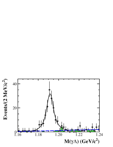
Figure 5: The $M(\gamma\Lambda)$ distribution, where the dots with error bars are data, the shaded histogram is the background contribution estimated from the inclusive MC sample, and the solid and dashed lines are the fit results for the overall and background components, respectively.

To determine the $\psi(3686)\rightarrow K^{-}\Sigma^{0}\bar{\Xi}^{+}$ yield, an extended unbinned maximum likelihood fit of the $M(\gamma\Lambda)$ distribution is performed with a double Gaussian function for the $\Sigma^{0}$ together with a first order Chebychev polynomial for the background shape. The overall fit result and the background component are shown in Fig. 5 with solid and dashed lines, respectively. The fit yields the number of $\Sigma^{0}$ events to be 142.5$\pm$13.0, and the resulting branching fraction is $\mathcal{B}(\psi(3686)\rightarrow K^{-}\Sigma^{0}\bar{\Xi}^{+})=(3.67\pm 0.33)\times 10^{-5}$, by taking the detection efficiency of 9.0% obtained from MC simulation and the branching fractions of intermediate states pdg in consideration. The errors are statistical only.

IV.2 STUDY OF $\bm{\chi_{cJ}\rightarrow K^{-}\Lambda\bar{\Xi}^{+}\ (J=0,\ 1,\ 2)}$

The $\chi_{cJ}\rightarrow K^{-}\Lambda\bar{\Xi}^{+}\ (J=0,\ 1,\ 2)$ yields are determined by fitting the invariant mass distribution of $K^{-}\Lambda\bar{\Xi}^{+}$, $M(K^{-}\Lambda\bar{\Xi}^{+})$. To remove the background from $\psi(3686)\rightarrow K^{-}\Sigma^{0}\bar{\Xi}^{+}$, the additional selection $M(\gamma\Lambda)>1.21$ GeV/$c^{2}$ is applied. The $M(K^{-}\Lambda\bar{\Xi}^{+})$ distribution is shown in Fig. 6, where the $\chi_{cJ}$ peaks are observed clearly. Potential backgrounds are studied using the events in the $\Lambda$ or $\bar{\Xi}^{+}$ sideband regions of data and the inclusive MC samples. The inclusive MC $M(K^{-}\Lambda\bar{\Xi}^{+})$ distribution is shown in Fig. 6 as the shaded histogram. According to the MC study, the dominant backgrounds are from the cascade decays $\psi(3686)\to\pi^{+}\pi^{-}J/\psi,J/\psi\to pK^{-}\bar{\Sigma}^{0},\bar{\Sigma}^{0}\to\gamma\bar{\Lambda}$ and $\psi(3686)\to K^{-}p\pi^{-}\bar{p}\pi^{+}\pi^{+}$, but none of them produce peak in the $\chi_{cJ}$ regions.

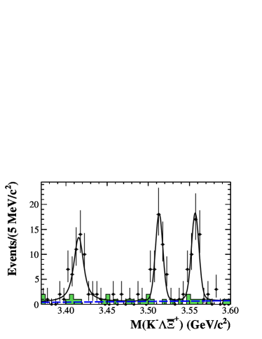
Figure 6: The $K^{-}\Lambda\bar{\Xi}^{+}$ mass distribution, where the dots with error bars are data, the shaded histogram is the background contribution estimated from the inclusive MC sample, and the solid and dashed lines are the overall and background component contributions from the fit.

An extended unbinned maximum likelihood fit of the $M(K^{-}\Lambda\bar{\Xi}^{+})$ distribution is performed to determine the number of $\chi_{cJ}$ events. The $\chi_{cJ}$ resonances are described by Breit-Wigner functions convoluted with Gaussian functions to account for the mass resolution, and the background is described by a first order Chebychev polynomial function. The fit results are shown as the solid curve in Fig. 6, and the yields of $\chi_{cJ}$ $(J=0,\ 1,\ 2)$ are 56.9$\pm$8.9, 48.5$\pm$7.4 and 50.8$\pm$7.8 events, respectively. Taking the detection efficiencies, 6.9%, 8.5% and 6.9% for $\chi_{cJ}$ $(J=0,\ 1,\ 2)$ estimated by MC simulation, and the branching fractions of the decays of intermediate states pdg into consideration, the product branching fractions $\mathcal{B}(\psi(3686)\to\gamma\chi_{cJ})\times\mathcal{B}(\chi_{cJ}\to K^{-}\Lambda\bar{\Xi}^{+})$ are measured to be $(1.90\pm 0.30)\times 10^{-5}$, $(1.32\pm 0.20)\times 10^{-5}$ and $(1.68\pm 0.26)\times 10^{-5}$ for $\chi_{cJ}$ ($J=0,\ 1,\ 2$), respectively. The errors are statistical only.

V SYSTEMATIC UNCERTAINTY

The different sources of systematic uncertainties for the measurement of branching fractions are considered and described below.

Tracking efficiency

In the analysis, both the proton and pion are from long lived particles ($\Lambda$ or $\Xi^{-}$), and the corresponding tracking efficiencies are studied using a clean $\Lambda$ control sample, selected by requiring the invariant mass recoiling against the $\bar{p}K^{+}$ system to be within the $\Lambda$ mass region in the decay $J/\psi\to\Lambda\bar{p}K^{+}$. The invariant mass recoiling against the $\bar{p}K^{+}\pi^{-}$ ($\bar{p}K^{+}p$) system is further required to be within the proton (pion) mass region to improve the purity of the control sample. The uncertainty of the tracking efficiency is estimated by the difference between efficiencies in data and MC samples and is parameterized as a function of transverse momentum. The average uncertainty of the proton (pion) tracking efficiency is estimated to be 1% (1%) by weighting with the transverse momentum distribution of the signal. The uncertainty of the $K^{\pm}$ tracking efficiency is studied with a clean control sample of $J/\psi\to K^{*}(892)^{0}K_{S}^{0},K^{*}(892)^{0}\to K^{\pm}\pi^{\mp}$, and the systematic uncertainty is estimated to be $1\%$ gpkl .

PID efficiency

Similarly, the PID efficiencies of $p/\bar{p}$ and $K^{\pm}$ are estimated using the same control samples as those in tracking efficiency studies. All tracks are reconstructed and the target one is allowed to be unidentified. The systematic uncertainties for $p$, $\bar{p}$ and $K^{\pm}$ are all found to be 1%.

Photon detection efficiency:

The photon detection efficiency is studied utilizing the control samples $\psi(3686)\to\pi^{+}\pi^{-}J/\psi$, $J/\psi\to\rho^{0}\pi^{0}$ and $\psi(3686)\to\pi^{0}\pi^{0}J/\psi$ with $J/\psi\to l^{+}l^{-}\ (l=e,\ \mu)$ and $\rho^{0}\pi^{0}$. The corresponding systematic uncertainty is estimated by the difference of detection efficiency between data and MC samples, and 1% is assigned for each photon chicv .

The secondary vertex fit:

The efficiencies of the secondary vertex fits for $\Lambda$ and $\Xi^{-}$ are investigated by the control samples $J/\psi\to\Lambda\bar{p}K^{+}$ and $J/\psi\to\Xi^{-}\bar{\Xi}^{+}$. The differences of efficiencies between data and MC samples are found to be 1%, and are taken as the systematic uncertainties.

Kinematic fit

The track helix parameters ($\phi_{0}$, $\kappa$, $\tan\lambda$) for MC samples are corrected to reduce the difference of the $\chi^{2}_{4C}$ distributions between data and MC gyp . The corresponding correction factors for kaons and the tracks from $\Lambda$ decay (proton and pion) are obtained from a clean sample $J/\psi\to\Lambda\bar{p}K^{+}$, and those for the tracks from $\Xi^{-}$ decay are obtained from the sample $J/\psi\to\Xi^{-}\bar{\Xi}^{+}$. The systematic uncertainties related to the 4C-fit, 1%, are estimated by the difference of efficiency between MC samples with and without the track helix parameter corrections.

Table 2: Summary of the relative systematic uncertainties (in %) in the branching fraction measurements. Here $K\Lambda\Xi$, $K\Sigma^{0}\Xi$, $\chi_{cJ}$ and $\Xi^{*-}\bar{\Xi}^{+}$ denote $\psi(3686)\rightarrow K^{-}\Lambda\bar{\Xi}^{+}$, $\psi(3686)\rightarrow K^{-}\Sigma^{0}\bar{\Xi}^{+}$, $\psi(3686)\rightarrow\gamma\chi_{cJ},\ \chi_{cJ}\rightarrow K^{-}\Lambda\bar{\Xi}^{+}$ and $\psi(3686)\to\Xi(1690/1820)^{-}\bar{\Xi}^{+},\Xi(1690/1820)^{-}\to K^{-}\Lambda$, respectively.

Source	$K\Lambda\Xi\$	$K\Sigma^{0}\Xi\$	$\chi_{cJ}\$	$\Xi^{*-}\bar{\Xi}^{+}$
Tracking	6	6	6	4
PID	3	3	3	3
$\Lambda$ vertex fit	1	1	1	1
$\Xi$ vertex fit	1	1	1	–
Kinematic fit	1	1	1	–
Photon detection	–	1	1	–
Signal model	2.1	0.5	1.1,3.0,2.4	0.8,1.6
Background shape	1.6	0.5	0,1.5,0.6	7.1,7.1
Fit range	1.6	1.9	0.2,0.1,0.2	6.3,4.4
Mass shift, resolution	–	–	–	0.6,0.4
Mass windows	2.9	1.4	3.2,2.3,1.8	1.0,1.3
$\mathcal{B}(\Lambda\to p\pi^{-})$	0.8	0.8	0.8	0.8
$\mathcal{B}(\bar{\Xi}^{+}\to\bar{\Lambda}\pi^{+})$	0.035	0.035	0.035	0.035
$\mathcal{B}(\bar{\Lambda}\to\bar{p}\pi^{+})$	0.8	0.8	0.8	0.8
$\mathcal{B}(\psi(3686)\to\gamma\chi_{cJ})$	–	–	3.2,4.3,4.0	–
$N_{\psi(3686)}$	0.8	0.8	0.8	0.8
Total	8.2	7.6	8.5,9.3,8.7	11.0,10.1

Table 3: Summary of the systematic uncertainties on $\Xi^{*-}$ parameters.

	$\Xi(1690)^{-}$		$\Xi(1820)^{-}$
	$M$ (MeV/$c^{2}$)	$\Gamma$ (MeV)	$M$ (MeV/$c^{2}$)	$\Gamma$ (MeV)
Signal model	0.2	0.3	1.5	1.2
Background shape	0.3	1.8	0.5	3.3
Fit range	0.3	1.7	0.2	2.2
Mass shift, resolution	0.5	0.8	0.2	0.2
Mass windows	0.7	0.7	0.4	0.6
Total	1.0	2.7	1.6	4.2

The fit method:

The systematic uncertainties related to the fit method are considered according to the following aspects. (1) The signal line-shapes: In the measurements of $\mathcal{B}(\psi(3686)\rightarrow K^{-}\Lambda\bar{\Xi}^{+})$, $\mathcal{B}(\chi_{cJ}\to K^{-}\Lambda\bar{\Xi}^{+})$ and $\mathcal{B}(\psi(3686)\rightarrow K^{-}\Sigma^{0}\bar{\Xi}^{+})$, the signal line-shapes are replaced by alternative fits using MC shapes, and the changes of yields are assigned as the systematic uncertainties. In the measurements of $\mathcal{B}(\psi(3686)\to\Xi^{*-}\bar{\Xi}^{+})$, the corresponding uncertainties mainly come from the uncertainty of $Q_{0}$. Alternative fits varying the $Q_{0}$ values within one standard deviation focus are performed, and the changes of yields are treated as the systematic uncertainties. (2) The background line-shapes: In the measurements of $\mathcal{B}(\psi(3686)\rightarrow K^{-}\Lambda\bar{\Xi}^{+})$, $\mathcal{B}(\chi_{cJ}\to K^{-}\Lambda\bar{\Xi}^{+})$ and $\mathcal{B}(\psi(3686)\rightarrow K^{-}\Sigma^{0}\bar{\Xi}^{+})$, the background shapes are described with a first order Chebychev polynomial function in the fit. Alternative fits with a second order Chebychev polynomial function are performed, and the resulting differences of the yields are taken as the systematic uncertainties related to the background line-shapes. In the measurement of $\mathcal{B}(\psi(3686)\to\Xi^{*-}\bar{\Xi}^{+})$, an alternative fit with a reversed ARGUS function (rARGUS) , $F_{\text{rARGUS}}(m)=F_{\text{ARGUS}}(2m_{0}-m)$, for the non-resonant components is performed, where $m_{0}$ is the mass threshold of $K^{-}\Lambda$. The changes in the yields are taken as systematic uncertainties. (3) Fit range: Fits with varied fit ranges, i.e., by expanding/contracting the range by 10 MeV/$c^{2}$ and shifting left and right by 10 MeV/$c^{2}$, are performed. The resulting largest differences are treated as the systematic uncertainties. (4) Mass shift and resolution difference: In the measurement of branching fractions related to $\Xi^{*-}$, a Gaussian function $G(m,\mu,\sigma)$, which represents the $\Xi^{*-}$ mass resolution, is included in the fit, where the parameters of Gaussian function are evaluated from MC simulation. To estimate the systematic uncertainty related to the mass shift and resolution difference between data and MC simulation, a fit with a new Gaussian function with additional parameters, i.e., $G(m,\mu+\Delta\mu,\sigma+\Delta\sigma)$, is performed, and the resulting difference is taken as the systematic uncertainty. The additional values $\Delta\mu$ and $\Delta\sigma$ are estimated by the difference in the fit results of the $\Lambda$ and $\bar{\Xi}^{+}$ between data and MC simulation.

Mass window requirement:

The systematic uncertainties related to $\Lambda$ and $\bar{\Xi}^{+}$ mass window requirements are estimated by varying the size of the mass window, i.e. contracting/expanding by 2 MeV/$c^{2}$. The resulting differences of branching fractions are treated as the systematic uncertainties.

Other:

The systematic uncertainties of the branching fractions of the decays $\psi(3686)\to\gamma\chi_{cJ}$, $\Xi^{-}\to\Lambda\pi^{-}$ and $\Lambda\to p\pi^{-}$ are taken from the world average values pdg . The uncertainty in the number of $\psi(3686)$ events is 0.8%, which is obtained by studying inclusive $\psi(3686)$ decays psipNo . The uncertainty in the trigger efficiency is found to be negligible due to the large number of charged tracks trigger .

The different sources of systematic uncertainties in the measured branching fractions are summarized in Table 2. Assuming all of the uncertainties are independent, the total systematic uncertainties are obtained by adding the individual uncertainties in quadrature.

In the measurement of the $\Xi^{*-}$ resonance parameters, the sources of systematic uncertainty related to the fit method and the $\Lambda$ and $\bar{\Xi}^{+}$ mass window requirements are considered. The same methods as those used above are implemented, and the differences of the mass and width of $\Xi^{*-}$ are regarded as the systematic uncertainties and are summarized in Table 3. The total systematic uncertainties on $\Xi^{*-}$ resonance parameters obtained by adding the individual uncertainties in quadrature are shown in Table 3.

VI CONCLUSION

Using a sample of $1.06\times 10^{8}$ $\psi(3686)$ events collected with the BESIII detector, the processes of $\psi(3686)\rightarrow K^{-}\Lambda\bar{\Xi}^{+}$ and $\psi(3686)\rightarrow\gamma K^{-}\Lambda\bar{\Xi}^{+}$ are studied for the first time. In the decay $\psi(3686)\rightarrow K^{-}\Lambda\bar{\Xi}^{+}$, the branching fraction $\mathcal{B}(\psi(3686)\rightarrow K^{-}\Lambda\bar{\Xi}^{+})$ is measured, and two structures, around 1690 and 1820 MeV/$c^{2}$, are observed in the $K^{-}\Lambda$ invariant mass spectrum with significances of 4.9$\sigma$ and 6.2$\sigma$, respectively. The fitted resonance parameters are consistent with those of $\Xi^{-}(1690)$ and $\Xi^{-}(1820)$ in the PDG pdg within one standard deviation. The measured masses, widths, and product decay branching fractions $\mathcal{B}(\psi(3686)\to\Xi^{*-}\bar{\Xi}^{+})\times\mathcal{B}(\Xi^{*-}\to K^{-}\Lambda)$ are summarized in Table 1. This is the first time that $\Xi^{-}(1690)$ and $\Xi^{-}(1820)$ hyperons have been observed in charmonium decays. In the study of the decay $\psi(3686)\rightarrow\gamma K^{-}\Lambda\bar{\Xi}^{+}$, the branching fractions $\mathcal{B}(\psi(3686)\rightarrow K^{-}\Sigma^{0}\bar{\Xi}^{+})$ and $\mathcal{B}(\chi_{cJ}\to K^{-}\Lambda\bar{\Xi}^{+})$ are measured. All of the measured branching fractions are summarized in Table 4. The measurements provide new information on charmonium decays to hyperons and on the resonance parameters of the hyperons, and may help in the understanding of the charmonium decay mechanism.

Table 4: Summary of the branching fractions measurements, where the first uncertainty is statistical and the second systematic.

Decay	Branching fraction
$\psi(3686)\rightarrow K^{-}\Lambda\bar{\Xi}^{+}$	$(3.86\pm 0.27\pm 0.32)\times 10^{-5}$
$\psi(3686)\to\Xi(1690)^{-}\bar{\Xi}^{+},\ \Xi(1690)^{-}\to K^{-}\Lambda$	$(5.21\pm 1.48\pm 0.57)\times 10^{-6}$
$\psi(3686)\to\Xi(1820)^{-}\bar{\Xi}^{+},\ \Xi(1820)^{-}\to K^{-}\Lambda$	$(12.03\pm 2.94\pm 1.22)\times 10^{-6}$
$\psi(3686)\rightarrow K^{-}\Sigma^{0}\bar{\Xi}^{+}$	$(3.67\pm 0.33\pm 0.28)\times 10^{-5}$
$\psi(3686)\to\gamma\chi_{c0},\ \chi_{c0}\to K^{-}\Lambda\bar{\Xi}^{+}$	$(1.90\pm 0.30\pm 0.16)\times 10^{-5}$
$\psi(3686)\to\gamma\chi_{c1},\ \chi_{c1}\to K^{-}\Lambda\bar{\Xi}^{+}$	$(1.32\pm 0.20\pm 0.12)\times 10^{-5}$
$\psi(3686)\to\gamma\chi_{c2},\ \chi_{c2}\to K^{-}\Lambda\bar{\Xi}^{+}$	$(1.68\pm 0.26\pm 0.15)\times 10^{-5}$
$\chi_{c0}\to K^{-}\Lambda\bar{\Xi}^{+}$	$(1.96\pm 0.31\pm 0.16)\times 10^{-4}$
$\chi_{c1}\to K^{-}\Lambda\bar{\Xi}^{+}$	$(1.43\pm 0.22\pm 0.12)\times 10^{-4}$
$\chi_{c2}\to K^{-}\Lambda\bar{\Xi}^{+}$	$(1.93\pm 0.30\pm 0.15)\times 10^{-4}$

VII ACKNOWLEDGMENTS

The BESIII collaboration thanks the staff of BEPCII and the IHEP computing center for their strong support. This work is supported in part by National Key Basic Research Program of China under Contract No. 2015CB856700; Joint Funds of the National Natural Science Foundation of China under Contracts Nos. 11079008, 11179007, U1232201, U1332201; National Natural Science Foundation of China (NSFC) under Contracts Nos. 10935007, 11121092, 11125525, 11235011, 11322544, 11335008, 11375204, 11275210; the Chinese Academy of Sciences (CAS) Large-Scale Scientific Facility Program; CAS under Contracts Nos. KJCX2-YW-N29, KJCX2-YW-N45; 100 Talents Program of CAS; INPAC and Shanghai Key Laboratory for Particle Physics and Cosmology; German Research Foundation DFG under Contract No. Collaborative Research Center CRC-1044; Istituto Nazionale di Fisica Nucleare, Italy; Ministry of Development of Turkey under Contract No. DPT2006K-120470; Russian Foundation for Basic Research under Contract No. 14-07-91152; U. S. Department of Energy under Contracts Nos. DE-FG02-04ER41291, DE-FG02-05ER41374, DE-FG02-94ER40823, DESC0010118; U.S. National Science Foundation; University of Groningen (RuG) and the Helmholtzzentrum fuer Schwerionenforschung GmbH (GSI), Darmstadt; WCU Program of National Research Foundation of Korea under Contract No. R32-2008-000-10155-0.

References

(1)
R. Horgan, Nucl. Phys. B 71, 514 (1974);
M. Jones, R.H. Dalitz, R. Horgan, Nucl. Phys. B 129, 45 (1977).
(2)
K. A. Olive et al., Chin. Phys. C 38, 1 (2014).
(3)
C. Dionisi et al., Phys. Lett. B 80, 145 (1978).
(4)
S. F. Biagi et al., Z. Phys. C 9, 305 (1981);
S. F. Biagi et al., Z. Phys. C 34, 15 (1987).
(5)
M. I. Adamovich et al., (WA89 Collaboration),
Eur. Phys. J. C 5, 621 (1998).
(6)
K. Abe et al., (Belle Collaboration),
Phys. Lett. B 524, 33 (2002).
(7)
B. Aubert et al., (BABAR Collaboration),
Phys. Rev. D 78, 034008 (2008).
(8)
J. B. Gay et al., Phys. Lett. B 62, 477 (1976).
(9)
N. Byers and S. Fenster, Phys. Rev. Lett. 11, 52 (1963).
(10)
S. F. Biagi et al., Z. Phys. C 34, 175 (1987).
(11)
M. Ablikim et al. (BESIII Collaboration),
Chin. Phys. C 37, 063001 (2013).
(12)
M. Ablikim et al. (BESIII Collaboration),
Chin. Phys. C 37, 123001 (2013).
(13)
M. Ablikim et al. (BESIII Collaboration),
Nucl. Instrum. Meth. A 614, 345 (2010).
(14)
S. Agostinelli et al. (GEANT4 Collaboration),
Nucl. Instrum. Meth. A 506, 250 (2003).
(15)
Z. Y. Deng et al. Chin. Phys. C 30, 371 (2006).
(16)
S. Jadach, B. F. L. Ward and Z. Was,
Comput. Phys. Commun. 130, 260 (2000).
(17)
S. Jadach, B. F. L. Ward and Z. Was,
Phys. Rev. D 63, 113009 (2001).
(18)
G. Karl et al. Phys. Rev. D 13, 1203 (1976);
P. K. Kabir and A. J. G. Hey, Phys. Rev. D 13, 3161 (1976).
(19)
D. J. Lange, Nucl. Instrum. Meth. A 462, 152 (2001);
R. G. Ping,
Chin. Phys. C 32, 599 (2008).
(20)
J. C. Chen, G. S. Huang, X. R. Qi, D. H. Zhang and Y. S. Zhu,
Phys. Rev. D 62, 034003 (2000).
(21)
M. Xu et al. Chin. Phys. C 33, 428 (2009).
(22)
B. S. Zou and D. V. Bugg,
Eur. Phys. J. A 16, 537 (2003).
(23)
J. M. Link et al. (FOCUS Collaboration),
Phys. Lett. B 621, 72 (2005).
(24)
M. Ablikim et al. (BESIII Collaboration),
Phys. Rev. D 87, 012007 (2013).
(25)
M. Ablikim et al. (BESIII Collaboration),
Phys. Rev. D 83, 112005 (2011).
(26)
M. Ablikim et al. (BESIII Collaboration),
Phys. Rev. D 87, 012002 (2013).
(27)
N. Berger, K. Zhu, Z. A. Liu, D. P. Jin, H. Xu, W. X. Gong, K. Wang and G. F. Cao,
Chin. Phys. C 34, 1779 (2010).