Orientation and Rotational Parameters of Asteroid 4179 Toutatis: New Insights from Chang’e-2’s Close Flyby

Abstract

In this work, we investigate the rotational dynamics of the ginger-shaped near-Earth asteroid 4179 Toutatis, which was closely observed by Chang’e-2 at a distance of $770\pm 120~{}$ meters from the asteroid’s surface during the outbound flyby (Huang et al., 2013a) on 13 December 2012. A sequence of high-resolution images was acquired during the flyby mission. In combination with ground-based radar observations collected over the last two decades, we analyze these flyby images and determine the orientation of the asteroid at the flyby epoch. The 3-1-3 Euler angles of the conversion matrix from the J2000 ecliptic coordinate system to the body-fixed frame are evaluated to be $-20.1^{\circ}\pm 1^{\circ}$, $27.6^{\circ}\pm 1^{\circ}$ and $42.2^{\circ}\pm 1^{\circ}$, respectively. The least-squares method is utilized to determine the rotational parameters and spin state of Toutatis. The characteristics of the spin-state parameters and angular momentum variations are extensively studied using numerical simulations, which confirm those reported by Takahashi et al. (2013). The large amplitude of Toutatis’ precession is assumed to be responsible for its tumbling attitude as observed from Earth. Toutatis’ angular momentum orientation is determined to be described by $\lambda_{H}=180.2^{+0.2^{\circ}}_{-0.3^{\circ}}$ and $\beta_{H}=-54.75^{+0.15^{\circ}}_{-0.10^{\circ}}$, implying that it has remained nearly unchanged for two decades. Furthermore, using Fourier analysis to explore the change in the orientation of Toutatis’ axes, we reveal that the two rotational periods are 5.38 and 7.40 days, respectively, consistent with the results of the former investigation. Hence, our investigation provides a clear understanding of the state of the rotational dynamics of Toutatis.

1 Introduction

The Apollo-type near-Earth asteroid (4179) Toutatis was originally discovered on 10 February 1934 and remained a lost asteroid until it was once again detected by C. Pollas and colleagues on 4 January 1989 in Caussols, France. From a dynamical viewpoint, the asteroid moves on an approximately 4:1 resonant orbit at a large eccentricity with the Earth and has passed through a close encounter with the Earth every four years since 1992 (Whipple et al., 1993; Krivova et al., 1994). Dating back to the decadal years of near-Earth flybys of the asteroid, the radar observations obtained from Arecibo and Goldstone reveal that Toutatis appears to be an irregularly shaped asteroid with two distinct lobes (Ostro et al., 1995; Hudson et al., 1998; Ostro et al., 1999, 2002; Hudson et al., 2003). Various types of ground-based observations indicate that Toutatis is a tumbling, non-principal axis (NPA)-rotating small body (Hudson et al., 1995; Ostro et al., 1999). These effects, as observed in Earth-approaching flybys, have also been reported based on optical observations and extensive radar measurements (Spencer et al., 1995; Hudson et al., 1995; Ostro et al., 1999; Takahashi et al., 2013).

The first near-Earth flyby for Toutatis occurred in December 1992 at a distance of 0.242 AU, when the asteroid again came into view. Optical observations were gathered from at least 25 sites around the world through an international campaign. The observed rotational light curves of Toutatis appeared to be highly unusual, with a large amplitude and a non-periodic long rotation period. Subsequently, Spencer et al. (1995) reported two major periods of complex rotation of approximately 7.3 and 3.1 days, as estimated from analysis of the data. In addition, they reported that Toutatis was the first asteroid to show strong photometric evidence of complex rotation. However, the authors did not clarify this complex rotation phenomenon.

Furthermore, radar observations were performed by Goldstone in California and by Arecibo Observatory during Toutatis’ approach in 1992. The delay-Doppler images achieved a spatial resolution of 19 meters in range and 0.15 millimeters per second in radial velocity. Ostro et al. (1995) suggested a rotational period between 4 and 5 days based on these radar data. According to the investigations of Burns et al. (1971, 1973), the damping timescale for the slow non-principal axis rotation of Toutatis exceeds the age of the solar system. Thus, Ostro et al. (1995) noted that the spin state of Toutatis may be primordial. However, recent investigation suggests that YORP effects may slow the spin states of asteroids. Thus, Toutatis’ spin state remains a mystery.

Based on these high-resolution delay-Doppler radar observations, Hudson et al. (1995) used a least-squares estimation to calculate Toutatis’ three-dimensional shape, spin states, and moment-of-inertia ratios. They showed that the dimensions along the three principal axes are 1.92, 2.40 and 4.60 kilometers and that Toutatis rotates in a long-axis mode. The two major periods were found to be 5.41 days for the rotation about the long principal axis and 7.35 days for the long-axis precession about the angular momentum vector. The results derived from the radar data were inconsistent with the solutions presented by Spencer et al. (1995).

Moreover, Hudson et al. (1998) adopted the published optical light curves (Spencer et al., 1995) and a radar-derived shape and spin-state model (Hudson et al., 1995) to estimate the Hapke parameters of Toutatis. The Hapke photometric model was applied, and a $\chi_{2}$ minimization proposed by Hudson et al. (1997) was performed. The synthetic light curves that were generated based on their model provided a good fit to the optical data, with an rms residual of 0.12 mag. They showed that the combination of the optical data and radar observations led to an estimation of the spin-state parameters for Toutatis that was superior to the radar-derived outcomes. The two parameters describing the moment-of-inertia ratios were determined to be 3.22 and 3.02, respectively.

Based on the triaxial ellipsoid shape and spin state given by Ostro et al. (1995), Kryszczynska et al. (1999) presented the results of modeling the light curve variations of this unusual rotating asteroid by numerically integrating Euler’s equation in combination with the explicit expression for an asteroid’s brightness as a function of Euler angles. They achieved good agreement between the observed and calculated light curves. They emphasized that the light curves of Toutatis were dominated by the precession effect and by the superposition of precession and rotation, which resulted in an unapparent relationship between the rotation period alone and the light curves. This understanding yielded an appropriate explanation for the inconsistency between the rotational period of Toutatis determined from optical data (Spencer et al., 1995) and that determined from radar observations (Hudson et al., 1995).

During the 1996 near-Earth approach, Toutatis was observed by the Goldstone 8510-MHz radar system. Based on the physical model derived from the observations of the 1992 approach, Ostro et al. (1999) analyzed the radar measurements and refined the estimates of the spin state of Toutatis. The combination of optical and radar data was proven to better predict the orientational sequence displayed in the images captured in 1996. After refinement, the two periods of Toutatis were updated and estimated to be $5.376\pm 0.001$ days for the rotation about the long principal axis and $7.420\pm 0.005$ days for the uniform precession of the long principal axis about the angular momentum vector. These two parameters yielded moment-of-inertia ratios of $3.22\pm 0.01$ and $3.09\pm 0.01$. Thus, the orientation at the 2004 approach could be predicted in both inertial and geocentric coordinate systems.

Scheeres et al. (2000) determined that mutual gravitational interactions between an asteroid and a planet or another asteroid can play a significant role in shaping the asteroid’s spin state. They analyzed the interactions of a sphere with an arbitrary mass and with Toutatis based on the radar-derived shape model. The results thus obtained could partially explain the phenomenon of Toutatis’ current unusual rotational state. It was demonstrated that the tumbling spin state of Toutatis might have been caused by near-Earth flybys over its lifetime. This hypothesis enabled the estimation of the mass distribution and moment-of-inertia for Toutatis (Busch et al., 2012), thereby allowing the likely internal structure to be inferred.

Using radar observations of five flybys from 1992 to 2008, Takahashi et al. (2013) modeled the rotational dynamics and estimated Toutatis’ spin-state parameters using the least-squares method. They calculated the Euler angles, angular velocities, and moment-of-inertia ratios as well as the center-of-mass (COM)-center-of-figure (COF) offset. By directly relating the COM-COF offset and the moment-of-inertia ratios to the spherical harmonic coefficients of the first- and second-degree gravity potential, they could determine the driving force of the external torque due to an external spherical body and evaluate the spin state. The terrestrial and solar tidal torques were considered in their dynamical models, and all aforementioned parameters were included in the variable state vector to be estimated in the study. Furthermore, the spin states and uncertainties were propagated to the 2012 flyby epoch.

On 13 December 2012, the first space-borne close observation of Toutatis was achieved by the second Chinese lunar probe, Chang’e-2, at a distance of $770\pm 120~{}(3\sigma)$ meters from Toutatis’ surface (Huang et al., 2013a). Optical images of the asteroid were acquired by one of the onboard engineering cameras during the outbound flyby. Through analysis of over 400 images, Huang et al. (2013a) estimated Toutatis’ osculating orbit, its dimensions along the major axes, and its orientations. The highest resolution of the images was better than 3 meters. New discoveries were made, including the presence of a giant depression at the large end, a sharply perpendicular silhouette near the neck region, and direct evidence of boulders and regoliths. The geological features suggest that Toutatis may have a rubble-pile structure. The physical length and width were determined to be $4.75\times 1.95~{}\rm{km}\pm~{}10\%$, respectively, and the direction of the $+z$ axis was calculated to be (234.1^∘, 60.7^∘). They showed that the bifurcated configuration may indicate that Toutatis is of contact binary origin and that it is composed of two major lobes (head and body).

In this work, we perform an extensive investigation of the optical images of Toutatis captured by Chang’e-2, and we determine the orientation of the asteroid at the flyby epoch. In combination with radar observations (Takahashi et al. (2013) and references therein), we estimate the rotational parameters of Toutatis. Moreover, the solar and terrestrial tidal torques are considered in the establishment of the rotational dynamics model. The torque due to the misalignment of the center of mass and the origin of the body-fixed frame is evaluated to be insignificant at first order (Hudson et al., 2003; Busch et al., 2012, 2014). Furthermore, we incorporate the external gravitational tidal effects from the Moon and Jupiter in our dynamical model.

Compared with the previous prediction (Takahashi et al., 2013), our results for Toutatis’ orientation, derived for Chang’e-2’s flyby epoch from both radar data and optical images, demonstrate good consistency with the observational results of the spacecraft (Huang et al., 2013a; Zou et al., 2014). Our simulations reproduce the trajectory of the long axis in space, with a precession amplitude of approximately $60^{\circ}$. This high amplitude of Toutatis’ precession is supportive of its tumbling attitude as observed from Earth. The characteristics of the angular momentum variations is investigated in detail, and the variation induced by the near-Earth flyby in 2004 is estimated to be $0.03\%$. The orientation of its angular momentum in space is found to be described by $\lambda_{H}=180.2^{+0.2^{\circ}}_{-0.3^{\circ}}$ and $\beta_{H}=-54.75^{+0.15^{\circ}}_{-0.10^{\circ}}$, and therefore, this orientation has remained nearly constant over the past two decades. The rotational periods are estimated from the simulations to be 5.38 and 7.40 days for the rotation and precession, respectively. These values are in good agreement with the work of Ostro et al. (1999).

This work is structured as follows: Section 2 presents the observational data, which comprise ground-based measurements and optical images acquired by Chang’e-2. In this section, we also analyze the optical data to derive the orientation of Toutatis at the flyby epoch. In Section 3, we model the rotational dynamics of Toutatis based on Euler’s equation. The least-squares and multiple shooting methods are employed to fit the variable state vector and the corresponding results. The simulation results are presented in Section 4. Finally, we conclude by discussing the innovations of our investigation compared with previous works.

2 Observations

As described above, Toutatis progrades on an approximately 4:1 resonant eccentric trajectory with the Earth. Orbital determination and rotational parameters for Toutatis have been documented since the asteroid began to be continually observed in 1992. Since that time, ground-based observations have been performed for its every near-miss of Earth. As is well known, on 13 Dec 2012, Chang’e-2 completed the first successful close flyby of Toutatis and acquired numerous images of this asteroid (Huang et al., 2013a).

Using the released data from the Minor Planet Center and hundreds of optical observations from the ground-based observational campaign that lasted from July to December of 2012, the orbital determination of Toutatis was precisely achieved within uncertainties on the order of several kilometers, and the orbital parameters at the flyby epoch were calculated to be $a$=2.5336 AU, $e$=0.6301, $i$=0.4466^∘, $\Omega$=124.3991^∘, $\omega$=278.6910^∘ and $M$=6.7634^∘. Hence, the initial orbit can be integrated to calculate the relative positions of Toutatis with respect to the Sun, Earth, Moon and other major planets in the solar system, which are required for computing the external torques from the solar tides, the terrestrial tides and the gravitational tides from other bodies.

The positions of the major planets and the Moon are calculated based on the DE405 ephemerides released by JPL . The gravitation of the Sun, the major planets and 67 asteroids in the main belt as well as post-Newtonian effects are considered in the dynamical model to achieve the orbital integration of Toutatis. In addition, Chebyshev polynomial fitting is numerically implemented to obtain the position of the asteroid at any given epoch.

2.1 Radar Measurements

Radar measurements of Toutatis acquired by Goldstone and Arecibo from 1992 to 2008 are used to solve for the asteroid’s rotational parameters. Takahashi et al. (2013) presented 33 sets of radar observations. Together with the orientation obtained by Chang’e-2 at the flyby epoch (see Section 2.2), we have 33 sets of ground-based observation outcomes, including Euler angles, angular velocities and one space-borne orientation parameter. The observational data are summarized in Table 1. The observational errors of the radar data are estimated to be between $3^{\circ}$ and $15^{\circ}$ (Takahashi et al., 2013) for the Euler angles and between 2^∘ day^-1 and 10^∘ day^-1 for the components of angular velocity; these errors are taken into account in our fitting.

Table 1: Observational data for Toutatis from 1992 to 2012 (Takahashi et al. (2013) and references therein).

Year	Month	Date	Hour	Minute	Second	Euler angles (∘)	Angular velocity (∘/day)
1992	12	2	21	40	0	(122.2, 86.5, 107.0)	(-35.6, 7.2, -97.0)
1992	12	2	19	30	0	(86.3, 81.8, 24.5)	(-16.4, -29.1,-91.9)
1992	12	4	18	10	0	(47.8, 60.7, 284)	(29.1, -23.2, -97.8)
1992	12	5	18	50	0	(14.6, 39.4, 207.1)	(33.3, 8.2, -92.9)
1992	12	6	17	30	0	(331.3, 23.7, 151.6)	(6.6, 34.5, -95.8)
1992	12	7	17	20	0	(222.5, 25.4, 143.9)	(12.8, 25.4, -104.1)
1992	12	8	16	40	0	(169.8, 45.5, 106.9)	(-31.1 -21.9, -97.7)
1992	12	9	17	50	0	(137.3, 71.3, 22.3)	(11.8, -36.9, -94.9)
1992	12	10	17	20	0	(103.1, 85.2, 292.6)	(35.8, -8.9, -97.9)
1992	12	11	9	40	0	(77, 85.7, 225.5)	(31, 17, -96.3)
1992	12	12	9	20	0	(42.8, 70.2, 133.2)	(-1.3, 37, -95.9)
1992	12	13	8	10	0	(13.7, 44.4, 51.9)	(-38.3, 17.9, -97.3)
1992	12	14	7	50	0	(323.7, 14, 0)	(-70.5, -50.6, -91.1)
1992	12	15	7	50	0	(193.2, 24.4, 21.4)	(22.1, -26.6, -96.6)
1992	12	16	7	10	0	(165.1, 46.4, 310.6)	(33.4, -3.4, -93.7)
1992	12	17	6	49	0	(130.6, 76.1, 234.9)	(12.6, 33.9, -94)
1992	12	18	7	9	0	(91.6, 81.6, 142.4)	(-24.3, 29.6, -102)
1996	11	25	19	48	0	(130.5, 78.9, 143.2)	(-32, 16.4, -98.2)
1996	11	26	17	51	0	(94.2, 88.1, 57.7)	(-30.6, -18.7, -91.5)
1996	11	27	17	34	0	(60.4, 81.2, 320.9)	(10.7, -36.8, -94.7)
1996	11	29	15	37	0	(349.3, 30, 168)	(23.1, 28.9, -98.3)
1996	11	30	15	47	0	(250.3, 14.2, 166.9)	(-18.6, 32.1, -94.9)
1996	12	1	14	23	0	(180.4, 37.6, 139.3)	(-38.7, -0.5, -98.1)
1996	12	2	13	43	0	(146.7, 64, 64.9)	(-12.6, -34.8, -97.9)
1996	12	3	12	20	0	(116.7, 81.4, 340.4)	(24.3, -28.2, -98.1)
2000	11	4	17	6	0	(110, 88.5, 30)	(0, -32.5, -98.9)
2000	11	5	18	1	0	(70.6, 84, 281)	(34.5, -17.2, -97.9)
2004	10	7	13	56	0	(79.19, 85.3, 365.2)	(-2.5, -35.4, -109)
2004	10	8	14	4	0	(44.9, 72.5, 263.1)	(32.4, -18.1, -97.9)
2004	10	9	13	57	0	(12.8, 47.3, 181.4)	(29.7, 22.8, -98.1)
2004	10	10	13	17	0	(327.7, 20.4, 124.1)	(-10.7, 34.7, -97.3)
2008	11	22	10	54	0	(119.5, 90.7, 92)	(118.1, 90.4, 93.6)
2008	11	23	10	45	0	(86.2, 85, 0.3)	(-0.4, -36.2, -98.9)
2012	12	13	8	30	0	(-20.1, 27.6, 42.2)

2.2 Observations by Chang’e-2

As mentioned previously, Chang’e-2 captured Toutatis’ silhouette via one of the onboard engineering cameras at the time when the asteroid was approaching the Earth in December 2012. The camera has a lens with a 54-mm focal length and a 1024-by-1024-pixel CMOS detector. The field of view of the camera is $7.2^{\circ}$ by $7.2^{\circ}$. The images were acquired during the outbound flyby of Chang’e-2 because of the large Sun-Toutatis-Chang’e-2 phase angle on the inbound route (Huang et al., 2013a; Zhao et al., 2014a). The imaging of Toutatis lasted approximately 25 minutes. Huang et al. (2013a) reported the first panoramic image of the asteroid in the sequence, which was acquired at a distance of 67.7 km from Toutatis at a resolution of 8.30 m, as shown in Figure 1a.

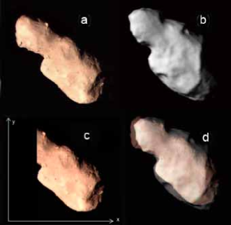
Figure 1: Images of Toutatis. a: First panoramic image captured by Chang’e-2. b: Best-matching attitude of the radar model with the optical image shown in Fig. 1a. c: Illustration of the graphical frame of the camera. d: Combination and comparison of the radar model with the optical results.

2.2.1 Attitude matching

The 3D shape model derived from delay-Doppler radar imaging, as presented in Figure 1b, is used to discern the attitude of Toutatis. The latest radar-derived shape model (Busch et al., 2012) was constructed based on additional radar measurements performed by Goldstone in 2000 and by Arecibo in 2004 and 2008, and in this work, this model is employed in combination with the optical images from Chang’e-2’s flyby to match the spin state of Toutatis.

In general, the attitude of a rigid body in space can be determined from its rotations about the three axes of an orthogonal coordinate system. As Figure 2 shows, to obtain the attitude of Toutatis, we suppose that the axes $l_{1}$, $l_{2}$ and $l_{3}$ are defined as follows: the mutually perpendicular axes $l_{1}$ and $l_{2}$ extend through the center of Toutatis’ shape and along the directions of the long short axes in the image, respectively. In addition, $l_{3}$ is perpendicular to the image plane through the intersection of $l_{1}$ and $l_{2}$, and thus, these axes form a right-handed coordinate system.

Considering the render and the orientation of the camera’s optical axis (Zhao et al., 2014a), the 3D radar-derived shape model of Toutatis can be rotated at an interval of $1^{\circ}$ for each of the three Euler angles about the three principal axes of its body-fixed frame to match its attitude to that shown in the optical images. As shown in Figure 2, we choose three criteria related to the optical image to determine whether the rotated model is consistent with the optical results from Chang’e-2’s view direction: (1) the slope of the long axis, represented by the red line in Figure 2a; (2) the ratio of the long axis to the short axis, indicated by the green line; and (3) the obvious topography on the neck area connecting the two major lobes of the asteroid, as shown in Figure 2b and 2c. These features of the optical image can be reproduced by rotating the 3D radar shape model about its three principle axes. Figure 1b shows the best approximation of the attitude of the radar model to that indicated by the optical image shown in Figure 1a. The two images are quantitatively compared in Table 2.

Table 2: Comparison of optical and radar image results.

Property	Optical Image	Radar Image
Slope	1.386	1.340
Ratio of length to width	2.52	2.08

Between the optical image and the model, the difference in the slope of $l_{1}$ is not obvious; however, the deviation in the ratio of the length to the width appears to be significant. Zou et al. (2014) suggested using a render frame with the lighting of the radar model and combining multiple optical images using computer graphics methods, which may yield a likely explanation for the higher value of the length-to-width ratio obtained for the optical images acquired by Chang’e-2.

Using the optical images from Chang’e-2, Bu et al. (2015) rotated the radar-derived model and retrieved an orientation with respect to the graphical frame described by direction cosine angles of $(126.13\pm 0.29^{\circ},122.98\pm 0.21^{\circ},126.63\pm 0.46^{\circ})$. In accordance with the definition of the cosine angles given by Bu et al. (2015), we calculate this set of cosine angles to be $(130.3\pm 1.0^{\circ},134.78\pm 1.0^{\circ},106.95\pm 1.0^{\circ})$. The two sets of results are quite similar to each other. However, we should note that the results presented here neglect the attitude of the camera in the inertial frame.

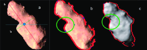
Figure 2: Properties of an optical image of Toutatis. a: The red line and green line represent the lengths of the image of the asteroid along the $l_{1}$ and $l_{2}$ directions, respectively; the ratio between these lengths is one of the properties that is used to characterize the image. The blue line represents the horizontal line, which can be used to determine the slope of $l_{1}$. b and c: The area within the green circle represents an obvious characteristic topological feature that can be used to derive information concerning the rotation about $l_{1}$.

2.2.2 Euler angles

Because of the fixed direction of the camera’s optical axis, Chang’e-2 maintained a nearly constant attitude throughout the shooting process. Figure 3 depicts the spacecraft’s body-fixed frame, where $\vec{l}$ is the direction of the camera’s optical axis and the corresponding unit vector in the spacecraft’s body-fixed frame is $(-0.06976,0.9976,0)$. The location relationship represents a transformation from Chang’e-2’s body-fixed frame to the graphical frame shown in Figure 1c. In combination with the attitude information of the spacecraft, we can establish a relationship between the graphical frame and the inertial coordinate system. As Figure 1c shows, the left portion of Toutatis is blocked by the solar panel on the spacecraft. The unit vectors of the x and y axes, which represent the horizontal and vertical axes in the graphical frame, are determined to be $(0.824,0.540,-0.173)$ and $(0.344,-0.233,0.910)$, respectively, in the J2000 equatorial coordinate system (Huang et al., 2013b).

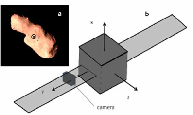
Figure 3: a. Graphical frame. b. Spacecraft’s body-fixed frame.

By merging the rotated radar-derived shape model and the optical image, Figure 1d illustrates the similarities and differences between the two models. In combination with the conversion relationship among the asteroid’s body-fixed frame, the graphical frame, and the inertial coordinate system, we can obtain the matrix describing the transformation from the J2000 ecliptic coordinate system to the asteroid’s body-fixed system expressed in terms of 3-1-3 Euler angles as below:

$$\vec{R}=R_{z}(42.2^{\circ})R_{x}(27.6^{\circ})R_{z}(-20.1^{\circ})\vec{r},$$ (1)

where $R_{x}$ and $R_{z}$ are the standard rotation matrices for right-handed rotations around the $X$ and $Z$ axes, respectively. The coordinate transformation and the corresponding Euler angles will be briefly introduced in the next section. The orientation of the principle axis is then obtained with respect to the attitude of the radar model, which is estimated to be ($249.87\pm 1^{\circ},62.43\pm 1^{\circ}$) in the J2000 ecliptic coordinate system (Zhao et al., 2014b). Corresponding errors arise from the matching process, the uncertainties of the radar-derived shape model and the attitude uncertainties of the spacecraft (Huang et al., 2013a).

3 Numerical Models

3.1 Dynamical Model

The rotation matrix shown in equation ($1$), which is composed of the three 3-1-3 Euler angles $\vec{\alpha}=(\alpha,\beta,\gamma)$, maps the information for conversion from the inertial coordinate system to the body-fixed frame, as shown in Figure 4. The body-fixed frame is generated by applying the following rotation sequence of the yaw, pitch and roll angles: a rotation of $\alpha$ around the z axis, then a rotation of $\beta$ around the x axis, and finally, a rotation of $\gamma$ around the z axis from the inertial frame.

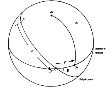
Figure 4: Coordinate system transformation relationship in terms of 3-1-3 Euler angles. Subscripts i and b indicate the inertial coordinate system and the body-fixed frame, respectively. The three angles $\alpha,\beta,$ and $\gamma$ form a 3-1-3 set of Euler angles.

The Euler angles describe the orientation of a rigid body in space at a specific time, and their variations represent spin states. Let the vector $\vec{\omega}$ define the instantaneous rotational velocity in the body-fixed frame. Then, the set of kinematic differential equations for the 3-1-3 Euler angles is as follows:

$$\dot{\vec{\alpha}}=\frac{1}{\sin\beta}\left(\begin{array}[]{c}~{}~{}~{}~{}\sin\gamma~{}~{}~{}~{}~{}~{}~{}~{}~{}~{}~{}\cos\gamma~{}~{}~{}~{}~{}~{}0\\ \cos\gamma\sin\beta~{}~{}~{}-\sin\gamma\sin\beta~{}~{}0\\ -\sin\gamma\cos\beta~{}~{}-\cos\gamma\cos\beta~{}~{}\sin\beta\end{array}\right)\vec{\omega}$$ (5)

$$=[B(\vec{\alpha})]\vec{\omega}~{}~{}.$$ (6)

The time derivative of the Euler angles encounters a singularity at either $\beta=0^{\circ}$ or $\beta=180^{\circ}$, which may cause $\alpha$ and $\gamma$ to rotate in the same plane.

As derived from the Euler equation, Euler’s rotational equation of motion describes the time derivative of the angular velocities:

$$[I]\dot{\vec{\omega}}=-[\tilde{\omega}][I]\vec{\omega}+\vec{L}~{}~{},$$ (7)

where the moment-of-inertia matrix $[I]$ is constant, symmetric and given in the body-fixed frame. It has dimensions of $[3\times 3]$ and can be defined in terms of six quantities. $\vec{L}$ represents the external torques acting on the dynamical system, and the matrix $[\tilde{\omega}]$ has the following form:

$$[\tilde{\omega}]=\left(\begin{array}[]{c}~{}~{}0~{}~{}~{}~{}~{}~{}~{}-\omega_{3}~{}~{}~{}\omega_{2}\\ ~{}~{}\omega_{3}~{}~{}~{}~{}~{}~{}~{}0~{}~{}~{}~{}-\omega_{1}\\ -\omega_{2}~{}~{}~{}~{}~{}\omega_{1}~{}~{}~{}~{}0\end{array}\right)~{}~{}.$$ (8)

Then, the time derivative of the angular velocities is expressed as follows:

$$\dot{\vec{\omega}}=[I]^{-1}(-[\tilde{\omega}][I]\vec{\omega}+\vec{L})~{}~{}.$$ (9)

To calculate the external torque exerted by a spherical body, we assume that $\vec{r}^{\prime}$ is the vector of an infinitesimal mass element $(dm)$ of the asteroid relative to the origin. Figure 5 presents a schematic diagram of the effect exerted by a spherical perturbing body on an irregularly shaped rigid body. According to the definition of angular momentum $\vec{H}$, we have

$$\frac{\rm{d}\vec{H}}{\rm{d}t}=\frac{\rm{d}}{\rm{d}t}\int dm~{}\vec{r}^{\prime}\times\dot{\vec{r}^{\prime}}=\int\vec{r}^{\prime}\times(d\vec{F}_{G}/dm-\ddot{\vec{B}})dm~{}~{},$$ (10)

where $\ddot{\vec{B}}$ is the acceleration of the origin in the inertial coordinate system and $d\vec{F}_{G}$ is the gravitational attraction experienced by an arbitrary mass element. When the center of mass of the rigid body is chosen as the origin $\bar{O}$, we have $\int dm\vec{r}^{\prime}\times\ddot{\vec{B}}=0$. Therefore, the torques exerted on the rigid body are written in the form (Schaub et al., 2009)

$$\vec{L}_{c}=\int_{M}\vec{r}^{\prime}\times d\vec{F}_{G}~{}~{}.$$ (11)

Otherwise, if the vector of $(dm)$ relative to the center of mass is $\vec{r}_{c}$, equation (6) has the following form:

$$\frac{\rm{d}\vec{H}}{\rm{d}t}=\int\vec{r}^{\prime}\times(d\vec{F}_{G}/dm-\ddot{\vec{B}})dm$$

$$=\int(\vec{r}_{c}-\vec{r}_{cm})\times(d\vec{F}_{G}/dm-\ddot{\vec{B}})dm~{}~{},$$ (12)

where $\vec{r}_{cm}=(x_{cm},y_{cm},z_{cm})^{T}$ is the vector of the center of figure with respect to the center of mass (the COM-COF offset). Thus, equation (6) can be expressed as follows:

$$\vec{L}=\int_{M}\vec{r}^{\prime}\times d\vec{F}_{G}+M\vec{r}_{cm}\times\ddot{\vec{B}}~{}~{},$$ (13)

where $M$ is the total mass of the asteroid.

Let $\vec{r}$ be the position vector of the spherical body relative to the asteroid. $\vec{R}=\vec{r}^{\prime}-\vec{r}$ denotes the position of a body element measured from the spherical body. Consequently, $d\vec{F}_{G}$ has the following form:

$$d\vec{F}_{G}=-\frac{GM_{s}}{R^{3}}\vec{R}dm~{}~{},$$ (14)

where $M_{s}$ is the mass of the external spherical body. Hence, the integral in equation (9) can be expressed as

$$\vec{L}=-GM_{s}\int_{M}\vec{r}^{\prime}\times\frac{\vec{R}}{R^{3}}dm+M\vec{r}_{cm}\times\ddot{\vec{B}}~{}~{}.$$ (15)

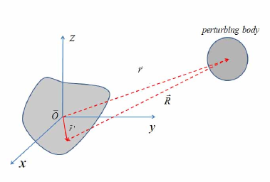
Figure 5: External torque of a spherical body on an irregularly shaped rigid body.

As Figure 5 shows, under the assumption that $\vec{r}\gg\vec{r}^{\prime}$, the first-order expansion of $\frac{\vec{R}}{R^{3}}$ has the following form:

$$\frac{\vec{R}}{R^{3}}=-[1+\frac{3(\vec{r}\cdot\vec{r}^{\prime})}{r^{2}}]\frac{\vec{r}}{r^{3}}+\frac{\vec{r}^{\prime}}{r^{3}}~{}~{}.$$ (16)

Substituting (12) into equation (9) allows the moment from the perturbing body to be divided into two components:

$$\vec{L}=\vec{L}_{1}+\vec{L}_{2}~{}~{},$$ (17)

where

$$\vec{L}_{1}=GM_{s}\int_{M}\vec{r}^{\prime}\times\frac{\vec{r}}{r^{3}}dm+M\vec{r}_{cm}\times\ddot{\vec{B}}~{}~{},$$ (18)

$$\vec{L}_{2}=\frac{3GM_{s}}{r^{5}}\int_{M}(\vec{r}\cdot\vec{r}^{\prime})(\vec{r}^{\prime}\times\vec{r})dm~{}~{}.$$ (19)

If the origin $\bar{O}$ is the center of mass of the irregularly shaped rigid body, then we obviously have $\vec{r}_{cm}\equiv 0$ and $\vec{L}_{1}\equiv 0$. Otherwise, truncated at the lowest order, we have

$$\ddot{\vec{B}}=\frac{GM_{s}}{M}\int_{M}\frac{\vec{r}}{r^{3}}dm~{}~{}.$$ (20)

If perturbing bodies other than the Sun are considered, then equation (16) should incorporate their contributions. Substituting equation (16) into equation (14), we obtain

$$\vec{L}_{1}=GM_{s}\int_{M}(\vec{r}^{\prime}+\vec{r}_{cm})\times\frac{\vec{r}}{r^{3}}dm$$

$$=GM_{s}\int_{M}\vec{r}_{c}\times\frac{\vec{r}}{r^{3}}dm=0~{}~{}.$$ (21)

Essentially, the torques imposed by the COM-COF offset are far too small to contribute in the first-order approximation. Furthermore, the change in angular momentum that results from $L_{1}$ is not an intrinsic feature of the rigid body; rather, it is determined solely by the selection of the base point when solving for the rotational dynamics.

Takahashi et al. (2013) expressed the second-degree potential as follows:

$$U_{2}=\frac{G}{2r^{3}}I_{T}-\frac{3G}{2r^{5}}\vec{r}[I]\vec{r}~{}~{},$$ (22)

where $I_{T}$ is the trace of $[I]$. The partial derivative of the potential can be derived as follows:

$$\frac{\partial{U_{2}}}{\partial\vec{r}}=-\frac{3G}{2r^{5}}I_{T}\vec{r}+\frac{15G}{2r^{7}}(\vec{r}[I]\vec{r})\vec{r}-\frac{3G}{r^{5}}[I]\vec{r}~{}~{};$$ (23)

therefore, the deduced moment can be expressed in the following form:

$$L_{2}=\frac{3GM_{s}}{r^{5}}[\tilde{r}][I]\vec{r}~{}~{}.$$ (24)

Our second-degree expansion of the moment given in equation (15) is consistent with the results represented by equation (20), which indicates that tidal torques caused by the oblateness of the rigid body.

3.2 Numerical Method

The least-squares and multiple shooting methods are used to fit the observational data and to simulate the propagation of the rotational parameters. The dynamical equation of the state vector, which is composed of three Euler angles and three angular velocities, is written as follows:

$$\dot{X}=F(X,t)~{}~{},$$ (25)

where $X=(\alpha,\beta,\gamma,\omega_{x},\omega_{y},\omega_{z})^{T}$; $\alpha$, $\beta$, and $\gamma$ are the 3-1-3 Euler angles, and $\omega_{1}$, $\omega_{2}$, and $\omega_{3}$ are the three components of angular velocity. The previous results for $I_{xx}$, $I_{yy}$, $I_{zz}$, $I_{xy}$, $I_{xz}$, and $I_{yz}$ are used in our calculations (Takahashi et al., 2013). $F$ is the function that represents the time derivative of $X$ and the dynamical model. In the first-order approximation, the dynamical model has the following form:

$$\dot{X}=A(X,t)X(t)~{}~{},$$ (26)

where $A(X,t)$ is the dynamical matrix. The transition matrix $\Phi$ is defined as follows:

$$\Phi(t_{1},t_{2})=\frac{\partial x(t_{1})}{\partial x(t_{2})}~{}~{}.$$ (27)

Based on the nominal orbit, we establish the relationship between the state vectors at two specific times, $t_{1}$ and $t_{2}$, as follows:

$$X(t_{2})=\phi(t_{1},t_{2})X(t_{1})~{}~{}.$$ (28)

Then, the transition matrix can be obtained by integrating the derivate equation:

$$\dot{\phi}(t_{0},t)=A(t,X)\phi(t_{0},t)~{}~{}.$$ (29)

The observational equation for the measurements $Y$ is

$$Y_{i}=Z(X_{i},t_{i})+\epsilon_{i}~{}~{},$$ (30)

where $Z$ represents the observational model, the subscript $i$ indicates the sequence of the observational data and $\epsilon$ represents the observational uncertainties. In the first-order approximation, the partial derivatives of the observational quantities with respect to the variables form the relationships between them, and we have

$$Y_{i}=\frac{\partial{Z}}{\partial{X}}|_{x=x_{i}}X_{i}+\epsilon_{i}=\frac{\partial{Z}}{\partial{X}}|_{x=x_{i}}\phi(t_{0},t_{i})X(t_{0})+\epsilon_{i}~{}~{},$$ (31)

where $t_{i}$ is the observation epoch of the data set. The least-squares method adopted herein is similar to that of Takahashi et al. (2013). The cost function is defined as follows:

$$J=\frac{1}{2}(Y-\frac{\partial{Z}}{\partial{X}}|_{x=x_{i}}\phi(t_{0},t_{i})X(t_{0}))^{T}W$$

$$(Y-\frac{\partial{Z}}{\partial{X}}|_{x=x_{i}}\phi(t_{0},t_{i})X(t_{0}))$$

$$+\frac{1}{2}(\bar{X}(t_{0})-X(t_{0}))^{T}\bar{P}^{-1}$$

$$(\bar{X}(t_{0})-X(t_{0}))~{}~{},$$

where $W$ is the weighting matrix, and $P$ is the covariance matrix. The bars over $X$ and $P$ represent the a priori values deduced through estimation or from previous results. The modified differential equation that computes the correction to the variables can be expressed as follows:

$$\triangle X(t_{0})=$$

$$(\sum H^{T}WH+\bar{P}^{-1})^{-1}(\sum H^{T}WY+\bar{P}^{-1}\bar{X}(t_{0}))^{-1}~{}~{}.$$ (33)

The RKF78 integrator can be used to integrate the rotational equations. The initial step size is set to approximately $10^{-9~{}\circ}$ for the Euler angles and $10^{-8~{}\circ}/day$ for the rotational velocities. In the integration, an adaptive step size is used to numerically solve the equations. The truncation errors for the Euler angles and rotational velocities are set to $10^{-8~{}\circ}$ and $10^{-7~{}\circ}/day$, respectively.

4 Results

To better understand the rotational dynamics of Toutatis, we performed a large number of numerical simulations based on Chang’e-2’s observations and ground-based radar measurements, using our dynamical models described above. In the following, we will present the major outcomes for the spin states, rotational period and variation in angular momentum of Toutatis.

In this work, the initial variables for Toutatis’ spin state that were used in our numerical simulations were adopted from Takahashi et al. (2013) for the epoch $t_{0}$ (17:49:47 UTC on 9 Nov 1992). The orientation of the angular momentum and the rotational periods were also calculated in the study. In our calculation, we balanced the weights of the optical data based on the uncertainties of the observations. Consequently, we derived innovative solutions for the spin state of Toutatis, which are summarized in Table 3.

Table 3: Spin-state parameters of Toutatis derived from our numerical simulations.

Property	Value
Simulated solutions at $t_{0}$	$\alpha=147.5^{\circ},\beta=63.9^{\circ},\gamma=241.5^{\circ}$
	$\omega_{1}=14.5^{\circ}/day,\omega_{2}=33.7^{\circ}/day,\omega_{3}=-98.5^{\circ}/day$
Results at flyby epoch	$\alpha=-3.65^{\circ},\beta=43.62^{\circ},\gamma=24.7^{\circ}$
Orientation of angular momentum	$\lambda_{H}=180.2^{+0.2^{\circ}}_{-0.3^{\circ}},\beta_{H}=-54.75^{+0.15^{\circ}}_{-0.10^{\circ}}$
Rotational/precession period	$5.38$ days, $7.40$ days

The residuals of the Euler angles (34 sets) and angular velocity (33 sets) were normalized with respect to the maximum radar observational errors ($15^{\circ}$ for the Euler angles and $10^{\circ}$/day for the angular velocities) and are shown in Figure 6. Because the previous prediction of the orientation at the Chang’e-2 flyby epoch based on the radar-derived results differs from that observed by Chang’e-2, the use of the optical data might have degraded the convergence of the simulation algorithm. Therefore, the magnitude of the residuals is larger than that observed in the results from the radar data (Takahashi et al, 2013). The residual errors in the simulations were normalized with respect to the observational uncertainties. Because of the inconsistency of the observational data, the magnitudes of the residuals are slightly higher than those of the previous results. However, all deviations lie within the $3\sigma$ region. The largest bias is found in the roll angle, which exhibits a remarkable difference between the prediction obtained from the radar measurements and the authentic spin state of Toutatis that is directly indicated by Chang’e-2’s observations at the flyby epoch.

Figure 6: Residuals of rotational parameters with respect to the maximum radar observational errors ( $15^{\circ}$ for the Euler angles and $10^{\circ}$/day for the angular velocities). Left panels: residuals of the Euler angles. Right panels: residuals of the angular velocity components.

4.1 Spin States

According to the numerical results derived from radar observations collected before 2008 (Busch et al., 2012), we considered a render effect for Toutatis and generated a predicted imaging outcome prior to Chang’e-2’s flyby, as shown in Figure 7a (Busch et al., 2012; Zhao et al., 2014a). In addition, based on the images acquired by Chang’e-2, we corrected the attitude of Toutatis by rotating the radar-derived shape model (see Section 2.2.1) to search for a good match with the Chang’e-2 images acquired at the flyby epoch (Fig. 7b), which provide the only space-borne optical data regarding Toutatis’ orientation. Furthermore, the present simulations yielded another solution for Toutatis’ attitude during the near-Earth flyby in 2012. Figure 7c shows the outcomes derived from our rotational model using space- and ground-based observations.

In comparison with the results obtained from the optical images (Fig. 7b), the radar-derived results (Fig. 7a) exhibit a dramatic deviation in the roll angle; hence, these results yield a different profile of the asteroid. The simulation results derived from our dynamical model (Fig. 7c) differ from those of Figure 7b with a pitch angle bias of within $20^{\circ}$. Thus, we may safely conclude that our outcomes represent a good improvement in the understanding of Toutatis’ spin state.

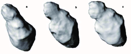
Figure 7: Comparison of Toutatis’ orientation. a: The left panel shows the results derived from Takahashi et al. (2013)’s work, with an uncertainty of dozens of degrees. b: The middle panel shows the results calculated from optical images acquired by Chang’e-2 and by rotating the radar shape model. c: The right panel presents the outcomes derived from our rotational model using space- and ground-based observations, which are close to those obtained from the optical images acquired by Chang’e-2.

The orientation of the long axis in the inertial frame likely reflects the precession of Toutatis. Based on the dynamical model of rotation, we calculated the variation in the direction of the long axis. Figure 8 shows the trajectories of the long axis with respect to the J2000 ecliptic coordinate system in a unit sphere over the past two decades. The motions of the long axis are projected onto the X-Y, X-Z and Y-Z planes (see Figs. 8a, 8b and 8c, respectively). The figure reveals that the long-axis motion of the asteroid has remained ellipsoidal in the X-Y and Y-Z planes, whereas it has rectilinearly precessed in the X-Z plane. All curves lie outside the ecliptic plane, implying that the small lobe of Toutatis is always located above the large end from a viewpoint close to the ecliptic.

Moreover, the orientation of the center axis of precession of Toutatis can be approximately determined from Figure 8, and the derived spherical coordinates can be estimated to be $(-0.2^{\circ},54.6^{\circ})$ in the ecliptic coordinate system. As a result of Toutatis’ clockwise rotation and precession, the center axis of precession points nearly along the opposite direction to the angular momentum (see Section 4.3). The amplitude of the precession is approximately $60^{\circ}$, which may shed light on the significantly different attitudes of the asteroid that have been observed from Earth.

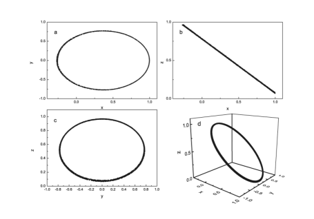
Figure 8: Trajectories in the J2000 ecliptic coordinate system of the long axis of Toutatis in a unit sphere. Panels a, b, and c show the trajectories in the X-Y, X-Z, and Y-Z planes, respectively, and panel d shows the motion of the long axis in 3D.

4.2 Angular Momentum

Considering the radar-derived shape model and the components of the inertial matrix inferred by Takahashi et al. (2013), we will now explore the angular momentum of Toutatis induced by various external gravitational torques. Figure 9 shows the variations in the external gravitational torques acting on the spin state of Toutatis from 1992 to 2012. The solar torque is on the order of $10^{-10}-10^{-7}$, indicating that its value is 2-3 orders higher at the perigee than at the apogee. Its periodic variation is clearly associated with Toutatis’ orbital period. The variation tendencies of the gravitational torques arising from the Earth and Moon are similar, as shown by the red and blue curves, respectively. There is a $10^{-2}$ difference in the orders of these torques because of the magnitudes of the masses of the bodies from which they arise. The periods of both torques are consistent with that of the black curve because of Toutatis’ resonance orbit with the Earth. At present, Toutatis is also in a 3:1 mean motion resonance orbit with Jupiter (Whipple et al., 1993); thus, one entire period of the torque induced by Jupiter is displayed by the green curve (Busch et al., 2014).

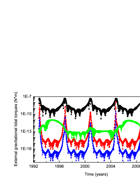
Figure 9: Variations in external gravitational torques. The black, red, blue, and green curves represent the torques arising from the Sun, the Earth, the Moon, and Jupiter, respectively.

Based on the rotational dynamical equation and the integrated orbit, the overall influence of these external torques on the variation in the magnitude of Toutatis’ rotational angular momentum from 1992 to 2012 was normalized with respect to the initial magnitude $H_{0}$ (Takahashi et al., 2013), as shown in Figure 10a. The terrestrial tidal torque (see the red curve in Fig. 10b) causes a considerable change in angular momentum when the asteroid approaches Earth at the perihelion or during the Earth flyby that occurs every four years. The most significant change, with a variation in angular momentum magnitude on the order of 0.03%, occurred in 2004 as a result of Toutatis passing the Earth within 4.02 lunar distances. Similarly, the tendency of the effect of the lunar torque is consistent with that of the terrestrial torque, as shown in Figure 10c. The solar tides always have a predominant influence on the rotational variation. However, the terrestrial tides also play an important role in the variation in angular momentum during Toutatis’ regular nearby visits to Earth. Figure 10d shows the influence on the angular momentum exerted by Jupiter. The order of magnitude of this effect slightly changed after the 2004 near-Earth flyby, and the amplitude continually remains lower than that of the terrestrial torque.

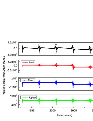
Figure 10: Variation in the angular momentum of Toutatis from 1992 to 2012.

As our simulation results indicate, the angular momentum orientation of Toutatis is determined to be described by ($\lambda_{H}=180.2^{+0.2^{\circ}}_{-0.3^{\circ}}$ and $\beta_{H}=-54.75^{+0.15^{\circ}}_{-0.10^{\circ}}$) and has remained nearly unchanged in space over the past two decades. Figure 11 shows the variations in Toutatis’ angular momentum orientation from 1992 to 2012 in the J2000 ecliptic frame. The amplitude of this change is shown to be less than one degree in both longitude and latitude. Jumps in the angular momentum orientation occur at the perihelion of each orbit. A small change in behavior is evident in Figure 11b as a result of the 2004 near-Earth flyby, consistent with Figure 10b. The variation with solar distance that is apparent in Figure 11c and 11d indicates that the solar and terrestrial torques predominantly affect the rotational motion of the asteroid. The misalignment of the curves in Figure 11d is also a result of the 2004 near-Earth flyby. Figure 11e and 11f show the angular momentum orientations of 33 sets of radar observations. Compared with the numerical results, the observation data fall within a reasonable error range, with the exception of a few points at large bias.

Figure 11: Variations in Toutatis’ angular momentum orientation from 1992 to 2012. Panels a and b show the variations in longitude and latitude versus time. Panels c and d show the change in longitude and latitude with the distance of Toutatis from the Sun. Panels e and f show the corresponding results from radar observations.

4.3 Rotational Period

The motions of the short or middle axis reflect the status of the rotation about the long axis, whereas the long axis’ motion represents precession. To calculate the two periods associated with the spin states of Toutatis, we determined the latitudinal variations of the asteroid’s long and middle axes in the J2000 ecliptic frame, as shown in Figure 12. We applied Fourier transform to analyze the periods of the two oscillation parameters and found that they are 5.38 days for the rotation about the principal axis and 7.40 days for the precession of the principal axis. These results are in good agreement with the previous results (Ostro et al., 1999).

Let $\beta_{X}$ and $\beta_{Z}$ indicate the latitudes of the asteroid’s long and middle axes, respectively, in the J2000 ecliptic coordinate system. Figures 12 and 13 show the latitudinal variations of these axes during the 1992 and 1996 flybys, respectively. Additionally, the numerical results (represented by dotted lines in Figs. 12 and 13) that were calculated from our dynamical model are found to be in good agreement with the radar observations within the error bars (marked by stars) (Takahashi et al., 2013), as listed in Table 4. Hence, we may conclude that the orientation parameters of Toutatis obtained from our investigation are very reliable. This evidence provides further confirmation that our proposed rotational model can be used to correctly evaluate the spin status of Toutatis or other asteroids.

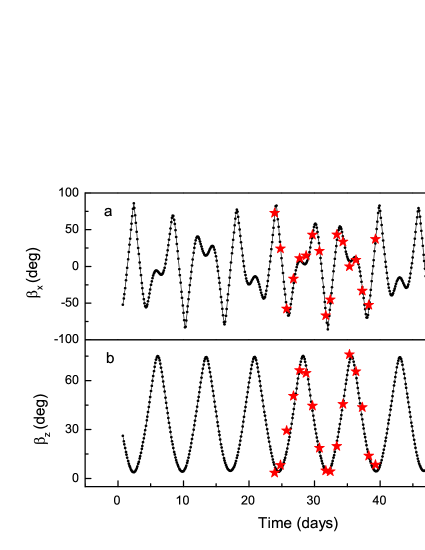
Figure 12: Latitudinal variations of Toutatis’ long axis $\beta_{z}$ and middle axis $\beta_{x}$ in the J2000 inertial coordinate system in 1992.

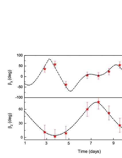
Figure 13: Latitudinal variations of Toutatis’ long axis $\beta_{z}$ and middle axis $\beta_{x}$ in the J2000 inertial coordinate system during the near-Earth flyby in 1996.

5 Conclusions and Discussions

In this work, we apply the observations collected during Chang’e-2’s outbound flyby to model the rotational dynamics and determine the spin state of Toutatis. Based on flyby images, we utilize the radar-derived shape model to calculate Toutatis’ orientation at the flyby epoch. In addition, we estimate the 3-1-3 Euler angles to be $-20.1^{\circ}\pm 1^{\circ}$, $27.6^{\circ}\pm 1^{\circ}$, and $42.2^{\circ}\pm 1^{\circ}$, respectively. Consequently, our results have greatly improved the estimation of the orientational parameters of Toutatis with respect to the previous predictions.

In combination with ground-based observations, we investigated the evolution of the spin parameters using numerical simulations. In addition to the solar and terrestrial torques, the tidal effects arising from the Moon and Jupiter are extensively considered in our dynamical model. The magnitude and influence of these gravitational torques were analyzed in this work. The solar tide appears to always be the dominant torque acting on the angular momentum of Toutatis. Furthermore, the contribution to the external gravitation torque due to the COM-COF offset appears to be negligible in the first-order approximation. We also found that the closest near-Earth flyby, at 4.02 lunar distances, resulted in a 0.03% change in the magnitude of the angular momentum of Toutatis. The dynamical influence exerted by Saturn on the angular momentum was also assessed in further simulations and found to be approximately $10^{2}$ lower than that of Jupiter. Hence, we can safely conclude that Saturn plays a less important role in the variation of Toutatis’ angular momentum.

The attitude at the Chang’e-2 flyby epoch that was derived from the numerical simulations yielded a better approximation to the optical results than that previously obtained from radar data alone. The largest deviation in the Euler angles is observed in the pitch angle, with a bias of less than $20^{\circ}$. The uncertainties corresponding to observational uncertainties and data processing error were considered in the simulations. The inconsistency in the different types of observational data may have led to higher residuals compared with previous results. Simulations based solely on radar observations were also performed, and the corresponding rms magnitude was much lower. However, the results obtained using a higher-accuracy dynamical model and a combination of the various types of observations yielded a good result that is highly consistent with the optical images acquired during the Chang’e-2 flyby in 2012.

The precession of Toutatis was investigated by considering the motion of its long axis. The behavior of the orbit in the inertial frame was found to be circular, with a center axis pointing along ($-0.2^{\circ},54.6^{\circ}$). The precession amplitude was estimated to be up to $60^{\circ}$, which may be responsible for the significantly different attitude of the asteroid as observed by ground-based facilities. Moreover, by exploring the motions of the long axis and middle axis, we determined the rotation period of Toutatis using Fourier analysis. The two major periods were found to be 5.38 days for the principal axis rotation and 7.40 days for the precession, in agreement with the results reported by Ostro et al. (1999).

Toutatis’ angular momentum orientation was determined to be described by $\lambda_{H}=180.2^{+0.2^{\circ}}_{-0.3^{\circ}}$ and $\beta_{H}=-54.75^{+0.15^{\circ}}_{-0.10^{\circ}}$, indicating that it has remained nearly unchanged for the last two decades. Because of the increasing magnitudes of the solar and terrestrial torques, tiny jumps in the angular momentum orientation occur at perihelion in each orbital period. However, the dynamical effects caused by the near-Earth flyby in 2004 slightly changed the latitude of Toutatis’ angular momentum orientation. Hence, our simulation results are in good agreement with previous radar observations. In a word, based on the combination of Chang’e-2’s observations and radar data, our investigation offers an improved understanding of the rotational dynamics of Toutatis.

References

- Bu et al. (2015) Bu Y.L., Tang G.S., Di K.C., et al., 2015, AJ, 149, 21
- Burns et al. (1971) Burns J.A., 1971, NASA Special Publication 267, 257
- Burns et al. (1973) Burns J.A., Safronov V., & Gold, T., 1973, MNRAS, 165, 403
- Busch et al. (2012) Busch M., Takahashi Y., Scheeres D.J., et al., 2012, AGU Fall Meeting Abstracts
- Busch et al. (2014) Busch M., Takahashi Y., Brozovic. M., et al., 2014, ACM meeting Abstracts
- Huang et al. (2013a) Huang J.C., Ji J.H., Ye P.J., et al., 2013a, Sci.Rep., 3,3411
- Huang et al. (2013b) Huang J.C., Wang X.L., Meng L.Z., et al., 2013b, Science China Technological Sciences,43, 596
- Hudson et al. (1995) Hudson R.S., Ostro S.J., Sci, 1995, 270, 84
- Hudson et al. (1997) Hudson R.S., Ostro S.J., Harris A.W., 1997, Icar, 130, 165
- Hudson et al. (1998) Hudson R.S., Ostro S.J., 1998, Icar, 135, 451
- Hudson et al. (2003) Hudson R.S., Ostro S.J., Scheeres D.J., 2003, Icar, 161, 346
- Krivova et al. (1994) Krivova N., Yagudina E., Shor V., 1994, PSS, 42, 741
- Kryszczynska et al. (1999) Kryszczynska A., Kwiatkowski T., Breiter S., Michalowski, T., 1999, A&A, 345, 643,
- Ostro et al. (1995) Ostro S.J., Hudson R.S., Jurgens R.F., et al., 1995, Sci, 270, 80
- Ostro et al. (1999) Ostro S.J., Hudson R.S., Rosema K.D., et al., 1999, Icar, 137, 122
- Ostro et al. (2002) Ostro S.J., Hudson R.S., Benner L.A., et al., 2002, Asteroids III, Univ. of Arizona Press, Tucson: 151
- Schaub et al. (2009) Schaub H., Junkins J.L., 2009, Analyatical Mechanics of Space System, American Institute of Aeronautics and Astronautics, Blacksburg
- Scheeres et al. (2000) Scheeres D.J., Ostro S.J., Werner R.A., Asphaug E., Hudson, R.S., 2000, Icar, 147, 106
- Spencer et al. (1995) Spencer J.R., Akimov L.A., Angeli C., et al., 1995, Icar, 117, 71
- Takahashi et al. (2013) Takahashi Y., Busch M.W., Scheeres D.J., 2013, AJ, 146, 95
- Whipple et al. (1993) Whipple A.L., Shelus P.J., 1993, Icar, 105, 408.
- Zhao et al. (2014a) Zhao Y.H., Wang S., Hu S.C., Ji J.H., 2014, ChA&A, 38, 163
- Zhao et al. (2014b) Zhao Y.H., Ji J. H., Hu S.C., 2014, The 40th COSPAR Scientific Assembly Abstracts
- Zou et al. (2014) Zou X., Li C., Liu J., et al., 2014, Icar, 229, 348