ON A CONJECTURE ON LINEAR SYSTEMS

Abstract.

In a remark to Green’s conjecture [Gre84], Paranjape and Ramanan analyzed the vector bundle $E$ which is the pullback by the canonical map of the universal quotient bundle $T_{\mbox{$\mathbb{P}$}^{g-1}}(-1)$ on $\mbox{$\mathbb{P}$}^{g-1}$ [PR88] and stated a more general conjecture [HPR92] and proved it for the curves with Clifford Index $1$ (trigonal and plane quintics). In this paper, we state the conjecture for general linear systems and obtain results for the case of hyperelliptic curves.

1. Introduction

Let $C$ be a smooth projective curve of genus $g\geq 2$ over a field $k$ and let $K$ be the canonical line bundle on $C$. In [Gre84], Green made a conjecture which relates two aspects Koszul cohomology (an algebraic aspect) and Clifford Index $\gamma_{C}$ (a geometric aspect) of a curve. This conjecture [Gre84] is equivalent to the following [PR88]: Let $E_{K}$ be the pullback by the canonical map $\Phi:C\rightarrow\mbox{$\mathbb{P}$}^{g-1}$ of universal quotient bundle on $\mbox{$\mathbb{P}$}^{g-1}$ . Then the map $\wedge^{i}\Gamma(C,E_{K})\rightarrow\Gamma(C,\wedge^{i}E_{K})$ is surjective $\forall$ $i\leq\gamma_{C}$. Paranjape and Ramanan [PR88] studied the vector bundle $E_{K}$ (stability properties). They also proved that all sections of $\wedge^{i}E_{K}$ which are locally decomposable are in the image of $\wedge^{i}\Gamma(E_{K})$ $\forall$ $i\leq\gamma_{C}$. Let $\sum_{i,K}$ be the cone of locally decomposable sections of $\wedge^{i}E_{K}$. In [HPR92], Hulek, Paranjape and Ramanan stated a conjecture.

Conjecture 1.1.

$\sum_{i,K}$ spans $\Gamma(\wedge^{i}E_{K})$ $\forall$ $i$ and for all curves.

This is stronger than Green’s conjecture. They proved it for curves with Clifford index $1$ (trigonal curves and plane quintics). Conjecture 1.1 is trivial in case of hyperelliptic curves, since $E_{K}$ is the $(g-1)$- fold direct sum of the hyperelliptic line bundle. Vector bundle $E_{K}$ is semi-stable (even stable if $C$ is not hyperelliptic). In a remark to conjecture made in [HPR92], Eusen and Schreyer [ES12] asked a more general question, whether $\Gamma(\wedge^{i}N)$ is spanned by locally decomposable sections holds for every (stable) globally generated vector bundle $N$ on every curve $C$. They gave counter examples to this more general question [ES12]. By broadening our view point, in this paper we state a conjecture for general linear systems. Let $C$ be a smooth curve of genus $g\geq 2$ and let $L$ be a globally generated line bundle on $C$. The evaluation map gives rise to an exact sequence

$$0\rightarrow E^{*}\rightarrow\Gamma(L)_{C}\rightarrow L\rightarrow 0$$

where $E^{*}$ is locally free of rank $h^{0}(L)-1$. Let $\sum_{i}$ be the cone of locally decomposable sections of $\wedge^{i}E$. We state

Conjecture 1.2.

$\sum_{i}$ spans $\Gamma(\wedge^{i}E)$ $\forall$ $i$ and for all curves.

In this paper we prove Conjecture 1.2 in case of hyperelliptic curves for the line bundles with degree large enough.

Theorem 1.

Let $C$ be a smooth hyperelliptic curve of genus $g\geq 2$ and let $L$ be a globally generated line bundle on $C$ of degree $d\geq 2g+1$ such that $H^{1}(L\otimes T^{-2})=0$, where $T$ is the hyperelliptic line bundle on $C$. The evaluation map gives rise to an exact sequence

(1) $$0\rightarrow E^{*}\rightarrow\Gamma(L)_{C}\rightarrow L\rightarrow 0$$

where $E^{*}$ is locally free of $\operatorname{rank}h^{0}(L)-1$. Let $\sum_{i}$ be the cone of locally decomposable sections of $\wedge^{i}E$. Then $\sum_{i}$ spans $\Gamma(\wedge^{i}E)$ $\forall$ $i$.

This work has been done as a part of my Ph.D thesis under the guidance of Prof. Kapil H. Paranjape. I gratefully acknowledge IISER Mohali, the host institution and University Grant Commission, India for the financial support during this period.

2. Geometry of the Hyperelliptic Curve

Since $C$ is hyperelliptic of genus $g\geq 2$. Thus $g^{1}_{2}$ on $C$ is unique. Let $\pi:C\rightarrow\mbox{$\mathbb{P}$}^{1}$ be the associated 2- sheeted covering, $T:=\pi^{*}\mathcal{O}_{\mbox{$\mathbb{P}$}^{1}}(1)$ is the unique $g^{1}_{2}$.
Consider the rank $2$ vector bundle $W$ on $\mbox{$\mathbb{P}$}^{1}$, where $W:=\pi_{*}L$.
Since,

$$\chi(L)=\chi(\pi_{*}L)$$

So,

$$d+1-g=rk(W)(\frac{degW}{rkW}+1-g_{\mbox{$\mathbb{P}$}^{1}})=2(\frac{degW}{2}+1)$$

which gives

$$degW=d-g-1$$

Thus,

$$detW \cong \mathcal{O}_{\mbox{$\mathbb{P}$}^{1}}(d-g-1)$$

$$W \cong W^{*}(d-g-1)$$

Since $\deg W=d-g-1$, thus there is a unique integer $x\leq\frac{d-g-1}{2}$ such that

(2) $$W\cong\mathcal{O}_{\mbox{$\mathbb{P}$}^{1}}(x)\bigoplus\mathcal{O}_{\mbox{$\mathbb{P}$}^{1}}(d-g-1-x)$$

Remark 1.

1. $x$ is the least integer such that

   $$H^{1}(W(-2-x))=H^{1}(\pi_{*}L(-2-x))=H^{1}(L\otimes T^{-2-x})\neq 0$$

   In particular, this implies that $\deg(L\otimes T^{-2-x})\leq 2g-2$ and thus we have

   $$\frac{d-2g-2}{2}\leq x\leq\frac{d-g-1}{2}$$

2. Since $H^{1}(L\otimes T^{-2})=0$, thus $x>0$, so we have

   $$max.\{1,\frac{d-2g-2}{2}\}\leq x\leq\frac{d-g-1}{2}$$

   which implies both $W$ and $W(-1)$ is globally generated.

3. Also, $H^{1}(L\otimes T^{-2})=0$ implies $H^{1}(L)=0$, thus by Riemann- Roch theorem, we have

   (3) $$h^{0}(L)=d-g+1$$

   and $\operatorname{rank}(E)=h^{0}(L)-1=d-g\geq 3$      (since $d\geq 2g+1$ and $g\geq 2$)

4. We have

   $$\Gamma(W(-1)) \cong \Gamma(\pi_{*}(L\otimes T^{-1}))$$

   $$\cong \Gamma(L\otimes T^{-1})$$

   $H^{1}(L\otimes T^{-2})=0$ gives $H^{1}(L\otimes T^{-1})=0$
   Thus, by Riemann-Roch theorem, we have
   

   $$h^{0}(L\otimes T^{-1})=d-g-1$$

   i.e., we have

   (4) $$h^{0}(W(-1))=d-g-1$$

Since $W(-1)$ is globally generated and $\Gamma(W)\cong\Gamma(L)$, so we have a surjection

$$\Gamma(L)_{\mbox{$\mathbb{P}$}^{1}}\rightarrow W\rightarrow 0,$$

which is an isomorphism for sections. Since $W(-1)$ is globally generated bundle on $\mbox{$\mathbb{P}$}^{1}$, $W$ is very ample, i.e., we get an inclusion

(5) $$\mbox{$\mathbb{P}$}(W^{*})\hookrightarrow\mbox{$\mathbb{P}$}(\Gamma(L)^{*}))=:\mbox{$\mathbb{P}$}.$$

Also we have a surjection

$$\pi^{*}W\rightarrow L\rightarrow 0$$

In other words, we have a subbundle of $\pi^{*}(W^{*})$ that is isomorphic to $L^{-1}$. This gives a morphism from $C$ to $\mbox{$\mathbb{P}$}(W^{*})$ with the property that the pullback of $\mathcal{O}_{W}(1)$ to $C$ is $L$. Also the composite of this morphism with the projection $p:\mbox{$\mathbb{P}$}(W^{*})\rightarrow\mbox{$\mathbb{P}$}^{1}$ is $\pi$. Since the induced map

$$\Gamma(\mbox{$\mathbb{P}$}(W^{*}),\mathcal{O}_{W}(1))\cong\Gamma(\mbox{$\mathbb{P}$}^{1},W)\rightarrow\Gamma(C,L)$$

is an isomorphism. Thus $C$ is actually embedded in $\mbox{$\mathbb{P}$}(W^{*})$. Let us denote the image of $\mbox{$\mathbb{P}$}(W^{*})$ in $\mathbb{P}$ by $S$. We return to the ruled surface $p:\mbox{$\mathbb{P}$}(W^{*})\rightarrow\mbox{$\mathbb{P}$}^{1}$. By (5), there is an embedding $\mbox{$\mathbb{P}$}(W^{*})\subset\mbox{$\mathbb{P}$}=\mbox{$\mathbb{P}$}(\Gamma(L)^{*})$ with hyperplane section $\tau=\mathcal{O}_{W}(1)$. Note that $\tau^{2}=\deg W=d-g-1$. Since $C$ is a secant ($2$-section) of $\mbox{$\mathbb{P}$}(W^{*})$, its class is of the form $\mathcal{O}_{W}(2)\otimes p^{*}\mathcal{O}_{\mbox{$\mathbb{P}$}^{1}}(m)$. To compute $m$, we note that $d=C.\tau=2\tau^{2}+m$. Thus $m=2g-d+2$.
Altogether, we have the following proposition

Proposition 2.1.

There are inclusions

$$C\subset S\subset\mbox{$\mathbb{P}$}$$

with the following properties:

1. the restriction of $\mathcal{O}_{\mbox{$\mathbb{P}$}}(1)$ to $S$ is $\mathcal{O}_{W}(1)$;

2. the restriction of $\mathcal{O}_{\mbox{$\mathbb{P}$}}(1)$ to $C$ is $L$;

3. both restrictions induce isomorphisms of the corresponding linear systems;

4. the divisor class on $S$ defined by $C$ is $\mathcal{O}_{W}(2)\otimes p^{*}\mathcal{O}_{\mbox{$\mathbb{P}$}^{1}}(-d+2g+2)$.

Notation: We will use the notation $U$ for the vector space $\Gamma(L\otimes T^{-1})$, i.e. we have

(6) $$\Gamma(W(-1))\cong U$$

and by (4), we have

(7) $$\dim U=d-g-1$$

3. Computation of dimensions

In order to prove the conjecture, we want to relate the sections of $\wedge^{i}E$ to the sections of a suitable vector bundle on $\mbox{$\mathbb{P}$}^{1}$

Lemma 3.1.

Let $F$ be a vector bundle on $\mbox{$\mathbb{P}$}^{1}$ that is globally generated. Then the evaluation sequence is

$$0\rightarrow\Gamma(F(-1))\otimes\mathcal{O}_{\mbox{$\mathbb{P}$}^{1}}(-1)\rightarrow\Gamma(F)_{\mbox{$\mathbb{P}$}^{1}}\rightarrow F\rightarrow 0$$

Proof: $F$ is a sum of line bundles of degree $\geq 0$. Thus remains to check for line bundles, which is easy.
∎

We want to apply this lemma to $W$ .

(8) $$0\rightarrow\Gamma(W(-1))\otimes\mathcal{O}_{\mbox{$\mathbb{P}$}^{1}}(-1)\rightarrow\Gamma(W)_{\mbox{$\mathbb{P}$}^{1}}\rightarrow W\rightarrow 0$$

Pulling back the evaluation sequence for $W$ on $\mbox{$\mathbb{P}$}^{1}$ to $C$ and using (6) and the fact that $\Gamma(\pi_{*}L)\cong\Gamma(L)$, we get

(9) $$0\rightarrow U\otimes T^{-1}\rightarrow\Gamma(L)_{C}\rightarrow\pi^{*}W\rightarrow 0$$

Also, we have a surjective map $\pi^{*}W\rightarrow L\rightarrow 0$, Let $Y$ be the kernel of $\pi^{*}W\rightarrow L\rightarrow 0$
i.e. we have

$$0\rightarrow Y\rightarrow\pi^{*}W\rightarrow L\rightarrow 0$$

$$\wedge^{2}(\pi^{*}W) \cong Y\otimes L$$

$$\pi^{*}(\wedge^{2}W) \cong Y\otimes L$$

$$\pi^{*}(\mathcal{O}_{\mbox{$\mathbb{P}$}^{1}}(d-g-1)) \cong Y\otimes L$$

$$T^{d-g-1} \cong Y\otimes L$$

$$Y \cong L^{-1}\otimes T^{d-g-1}$$

Thus, we have

(10) $$0\rightarrow L^{-1}\otimes T^{d-g-1}\rightarrow\pi^{*}W\rightarrow L\rightarrow 0$$

we get a following commutative diagram

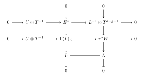
Figure 1.

where the left vertical map is the evaluation map.

Dualise the diagram in figure (1), we get

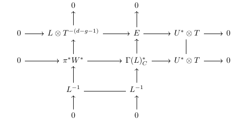
Figure 2.

The first line of commutative diagram in figure (2) gives rise to an exact sequence

(11) $$0\rightarrow L\otimes T^{-(d-g-1)}\otimes\wedge^{i-1}U^{*}\otimes T^{i-1}\rightarrow\wedge^{i}E\rightarrow\wedge^{i}U^{*}\otimes T^{i}\rightarrow 0$$

Since, $\pi^{*}W^{*}$ is a rank $2$ bundle we only get a filtration consisting of the following two exact sequences:

(12) $$0\rightarrow\wedge^{2}\pi^{*}W^{*}\otimes\wedge^{i-2}U^{*}\otimes T^{i-2}\rightarrow\wedge^{i}\Gamma(L)^{*}_{C}\rightarrow L_{i}\rightarrow 0$$

(13) $$0\rightarrow\pi^{*}W^{*}\otimes\wedge^{i-1}U^{*}\otimes T^{i-1}\rightarrow L_{i}\rightarrow\wedge^{i}U^{*}\otimes T^{i}\rightarrow 0$$

Since the second horizontal sequence of diagram in figure (2) is the pullback via $\pi$ of the dual of the sequence (8). Thus both the above sequences come from $\mbox{$\mathbb{P}$}^{1}$, i.e. there exists a vector bundle $L^{\prime}_{i}$ on $\mbox{$\mathbb{P}$}^{1}$, such that $L_{i}=\pi^{*}L^{\prime}_{i}$ and the sequences

(14) $$0\rightarrow\wedge^{2}W^{*}\otimes\wedge^{i-2}U^{*}\otimes\mathcal{O}(i-2)\rightarrow\wedge^{i}\Gamma(L)^{*}_{\mbox{$\mathbb{P}$}^{1}}\rightarrow L^{\prime}_{i}\rightarrow 0$$

(15) $$0\rightarrow W^{*}\otimes\wedge^{i-1}U^{*}\otimes\mathcal{O}(i-1)\rightarrow L^{\prime}_{i}\rightarrow\wedge^{i}U^{*}\otimes\mathcal{O}(i)\rightarrow 0$$

are such that (12) and(13) are pullback of (14) and (15) respectively.
Dualising (1), we have

$$0\rightarrow L^{-1}\rightarrow\Gamma(L)_{C}^{*}\rightarrow E\rightarrow 0$$

Thus the map $\wedge^{i}\Gamma(L)^{*}_{C}\rightarrow\wedge^{i}E$ is surjective.
Also we have $\wedge^{i}\Gamma(L)^{*}_{C}\rightarrow L_{i}\rightarrow 0$. The maps $\wedge^{i}\Gamma(L)^{*}_{C}\rightarrow\wedge^{i}E\rightarrow 0$ factors through $L_{i}=\pi^{*}L^{\prime}_{i}$. Thus we get the following commutative diagram with exact rows and columns:

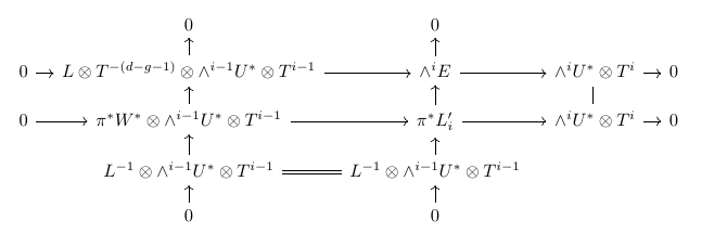
Figure 3.

where the top horizontal sequence is (11), middle horizontal sequence is (13), left vertical sequence is obtained by dualising (10) and tensoring it with $\wedge^{i-1}U^{*}\otimes T^{i-1}$.

Let us compute the dimensions of the spaces $\Gamma(L^{\prime}_{i})$ and $\Gamma(\wedge^{i}E)$ for $i\leq d-g$ ($=\operatorname{rank}E$)

Lemma 3.2.

When $d\geq 2g+1$, we have

$$\dim\Gamma(L^{\prime}_{i})=\bigl{(}\begin{smallmatrix}d-g+1\\ i\end{smallmatrix}\bigr{)}+\bigl{(}\begin{smallmatrix}d-g-1\\ i-2\end{smallmatrix}\bigr{)}(d-i-g)$$

for $i\leq d-g$

Proof: Consider (14)

$$0\rightarrow\wedge^{2}W^{*}\otimes\wedge^{i-2}U^{*}\otimes\mathcal{O}(i-2)\rightarrow\wedge^{i}\Gamma(L)^{*}_{\mbox{$\mathbb{P}$}^{1}}\rightarrow L^{\prime}_{i}\rightarrow 0$$

Since

$$detW\cong\mathcal{O}_{\mbox{$\mathbb{P}$}^{1}}(d-g-1).$$

Thus

$$detW^{*}\cong\mathcal{O}_{\mbox{$\mathbb{P}$}^{1}}(-(d-g-1))$$

Thus, we get

$$0\rightarrow\wedge^{i-2}U^{*}\otimes\mathcal{O}(i-d+g-1)\rightarrow\wedge^{i}\Gamma(L)^{*}\rightarrow L^{\prime}_{i}\rightarrow 0$$

Since,

$$i\leq d-g,h^{0}(\mathcal{O}(i-d+g-1))=0$$

Therefore,

$$h^{0}(L^{\prime}_{i})=h^{0}(\wedge^{i}\Gamma(L)^{*})+h^{1}(\wedge^{i-2}U^{*}\otimes\mathcal{O}(i-d+g-1))$$

By (7), we have

$$dimU=d-g-1$$

and by (3)

$$h^{0}(L)=d-g+1$$

$$h^{1}(\mathcal{O}(i-d+g-1))=d-i-g$$

Thus,

$$\dim\Gamma(L^{\prime}_{i})=\bigl{(}\begin{smallmatrix}d-g+1\\ i\end{smallmatrix}\bigr{)}+\bigl{(}\begin{smallmatrix}d-g-1\\ i-2\end{smallmatrix}\bigr{)}(d-i-g).$$

∎

3.1. Syzygies of the curve

The syzygies of canonically embedded curves were computed by Schreyer [Sch86]. Based on the parallel idea, we compute the syzygies of the curve $C$. For this, let

$$R=\bigoplus_{i=1}^{\infty}\Gamma(C,L^{i})$$

be the homogeneous coordinate ring of $C$ w.r.t $L$ and

$$S=Sym\Gamma(C,L)=\bigoplus_{n\geq 0}\Gamma(\mathcal{O}_{\mbox{$\mathbb{P}$}^{d-g}}(n)).$$

Let

(16) $$0\rightarrow F_{t}\rightarrow\cdots\rightarrow F_{0}\rightarrow R\rightarrow 0,$$

be a minimal free resolution of the graded $S$- module $R$. Then $F_{i}=\bigoplus_{j}S(-j)^{\beta_{ij}}=\bigoplus_{j}M_{ij}\otimes S(-j)$, where $M_{ij}$ is a $k$- vector space of $\dim\beta_{ij}$ and $S(-j)$ is the free $S$- module with one generator in degree $j$.
The resolution (16) is equivalent to the free resolution of $\mathcal{O}_{C}$ as an $\mathcal{O}_{\mbox{$\mathbb{P}$}^{d-g}}$- module:

$$0\rightarrow\bigoplus_{j}\mathcal{O}(-j)^{\beta_{d-g-1,j}}\rightarrow\cdots\rightarrow\bigoplus_{j}\mathcal{O}(-j)^{\beta_{0,j}}\rightarrow\mathcal{O}_{C}\rightarrow 0$$

To find this resolution, one starts with the exact sequence

$$0\rightarrow\mathcal{O}_{S}(-2\tau+(d-2g-2)f)\rightarrow\mathcal{O}_{S}\rightarrow\mathcal{O}_{C}\rightarrow 0$$

(see Proposition (2.1)). The idea is to first resolve the sheaves $\mathcal{O}_{S}$ and $\mathcal{O}_{S}(-2\tau+(d-2g-2)f)$ resp. as $\mathcal{O}_{\mbox{$\mathbb{P}$}^{d-g}}$ modules and then form a mapping cone . The result turns out to be a minimal resolution of $\mathcal{O}_{C}$.
Firstly, we will recall from [Eis05] the description of the syzygies of these sheaves.
Let $\xi=\mathcal{O}(e_{1})\bigoplus\mathcal{O}(e_{2})\bigoplus\cdots\bigoplus\mathcal{O}(e_{s})$ be a locally free sheaf of $\operatorname{rank}$ $s$ on $\mbox{$\mathbb{P}$}^{1}$, and let $p_{\xi}:\mbox{$\mathbb{P}$}(\xi)\rightarrow\mbox{$\mathbb{P}$}^{1}$ denote the corresponding $\mbox{$\mathbb{P}$}^{s-1}$ bundle. A rational normal scroll $X$ of type $S(e_{1},e_{2},\cdots,e_{s})$ with $e_{1}\geq e_{2}\geq\cdots\geq e_{s}\geq 0$ and

$$f=e_{1}+e_{2}+\cdots+e_{s}\geq 2$$

is the image of $\mbox{$\mathbb{P}$}(\xi)$ in $\mbox{$\mathbb{P}$}^{r}=\mbox{$\mathbb{P}$}(H^{0}(\mbox{$\mathbb{P}$}(\xi),\mathcal{O}_{\mbox{$\mathbb{P}$}(\xi)}(1)))$:

$$j:\mbox{$\mathbb{P}$}(\xi)\rightarrow X\subset\mbox{$\mathbb{P}$}^{r},r=f+s-1$$

The Picard group of $\mbox{$\mathbb{P}$}(\xi)$ is generated by the hyperplane class $H=[j^{*}\mathcal{O}_{\mbox{$\mathbb{P}$}^{r}}(1)]$ and the ruling $R=[p_{\xi}^{*}\mathcal{O}_{\mbox{$\mathbb{P}$}^{1}}(1)]$:

$$Pic\mbox{$\mathbb{P}$}(\xi)=\mbox{$\mathbb{Z}$}H\bigoplus\mbox{$\mathbb{Z}$}R,$$

the intersection product is given by

$$H^{s}=f,H^{s-1}.R=1,R^{2}=0.$$

We recall from [Eis05], the description of the syzygies of the sheaves

$$\mathcal{O}_{X}(aH+bR):=j_{*}\mathcal{O}_{\mbox{$\mathbb{P}$}(\xi)}(aH+bR),~{}~{}~{}a,b\in\mbox{$\mathbb{Z}$}$$

regarded as $\mathcal{O}_{\mbox{$\mathbb{P}$}^{r}}$- modules, at least in case $b\geq-1$.

Let

$$\Phi:F\rightarrow G$$

be a map of locally free sheaves of $\operatorname{rank}$ $f^{\prime}$ and $g^{\prime}$, $f^{\prime}\geq g^{\prime}$, respectively on a smooth variety $V$. We recall from [BE75] the family of complexes $\zeta^{b},b\geq-1$ of locally free sheaves on $V$, which resolve the $b^{th}$- symmetric power of coker $\Phi$ under suitable hypothesis on $\Phi$.
Define the $\j^{th}$ term in the complex $\zeta^{b}$ by

$$\zeta^{b}_{j}=\left\{\begin{array}[]{lll}\wedge^{j}F\otimes S_{b-j}G,&for&0\leq j\leq b\\ \wedge^{j+g^{\prime}-1}F\otimes D_{j-b-1}G^{*}\otimes\wedge^{g^{\prime}}G^{*},&for&j\geq b+1\\ \end{array}\right.$$

and differential

$$\zeta^{b}_{j}\rightarrow\zeta^{b}_{j-1}$$

by the multiplication with $\Phi\in H^{0}(V,F^{*}\otimes G)$ for $j\neq b+1$ and $\wedge^{g^{\prime}}\Phi\in H^{0}(V,\wedge^{g^{\prime}}F^{*}\otimes\wedge^{g^{\prime}}G)$ for $j=b+1$ in the appropriate term of the exterior $(\wedge F)$, symmetric (S.G) or divided power (D.G) algebra.

Proposition 3.3.

[Eis05] $\zeta^{b}(a)$ for $b\geq-1$ is the minimal resolution of $\mathcal{O}_{X}(aH+bR)$ as an $\mathcal{O}_{\mbox{$\mathbb{P}$}^{r}}$- module, where $\zeta^{b}(a)=\zeta^{b}\otimes\mathcal{O}_{\mbox{$\mathbb{P}$}^{r}}(a)$

3.2. Minimal Resolution of $\mathcal{O}_{C}$

We have

$$C\subset S\subset\mbox{$\mathbb{P}$}=\mbox{$\mathbb{P}$}(\Gamma(C,L)^{*})$$

$C$ is contained in a $2$- dimensional rational normal scroll $S$ of type $S(e_{1},e_{2})$ and degree $f=e_{1}+e_{2}=d-g-1\geq 2$.
$C$ is a divisor of class

$$C\sim 2H-(f-(g+1))R~{}~{}~{}~{}~{}on~{}~{}S$$

The mapping cone [Sch86]

$$\zeta^{f-(g+1)}(-2)\rightarrow\zeta^{0}$$

is the minimal resolution of $\mathcal{O}_{C}$ as an $\mathcal{O}_{\mbox{$\mathbb{P}$}^{d-g}}$- module.
We consider

$$\Phi:F\otimes\mathcal{O}_{\mbox{$\mathbb{P}$}^{d-g}}(-1)\rightarrow G\otimes\mathcal{O}_{\mbox{$\mathbb{P}$}^{d-g}}$$

be the map of locally free sheaves, where $F$ is a vector space of dimension $f=d-g-1$ and $G$ is a vector space of dimension $2$

Firstly, we will compute

$$\zeta^{f-(g+1)}(-2)=\zeta^{d-2g-2}\otimes\mathcal{O}(-2)$$

Now,

$$\zeta^{d-2g-2}_{j}=\left\{\begin{array}[]{ll}\wedge^{j}(F\otimes\mathcal{O}(-1))\otimes S_{d-2g-2-j}(G\otimes\mathcal{O}),&0\leq j\leq d-2g-2\\ \wedge^{j+1}(F\otimes\mathcal{O}(-1))\otimes D_{j-d+2g+2-1}(G\otimes\mathcal{O})^{*}\otimes\wedge^{2}(G\otimes\mathcal{O})^{*},&j\geq d-2g-1\\ \end{array}\right.$$

Since $j+1$ can be at most $d-g-1$. Thus, we have

$$\zeta^{d-2g-2}_{j}=\left\{\begin{array}[]{ll}\wedge^{j}(F\otimes\mathcal{O}(-1))\otimes S_{d-2g-2-j}(G\otimes\mathcal{O}),&0\leq j\leq d-2g-2\\ \wedge^{j+1}(F\otimes\mathcal{O}(-1))\otimes D_{j-d+2g+2-1}(G\otimes\mathcal{O})^{*}\otimes\wedge^{2}(G\otimes\mathcal{O})^{*},&d-2g-1\leq j\leq d-g-2\\ \end{array}\right.$$

$$\zeta^{d-2g-2}_{j}=\left\{\begin{array}[]{ll}\wedge^{j}(F\otimes\mathcal{O}(-1))\otimes S_{d-2g-2-j}(G\otimes\mathcal{O}),&0\leq j\leq d-2g-2\\ \wedge^{j}(F\otimes\mathcal{O}(-1))\otimes D_{j-d+2g}(G\otimes\mathcal{O})^{*}\otimes\wedge^{2}(G\otimes\mathcal{O})^{*},&d-2g-1\leq j\leq d-g-1\\ \end{array}\right.$$

Similarly we can compute $\zeta^{0}_{j}$,

$$\zeta^{0}_{j}=\left\{\begin{array}[]{ll}\wedge^{j}(F\otimes\mathcal{O}(-1))\otimes S_{0-j}(G\otimes\mathcal{O})&j=0\\ \wedge^{j+1}(F\otimes\mathcal{O}(-1))\otimes D_{j-1}(G\otimes\mathcal{O})^{*}\otimes\wedge^{2}(G\otimes\mathcal{O})^{*}&1\leq j\leq d-g-2\\ \end{array}\right.$$

The minimal free resolution of $\mathcal{O}_{C}$ is

(17) $$0\rightarrow\mathcal{O}(-(d-g-1))^{g}\rightarrow\cdots\rightarrow\wedge^{j+1}(F\otimes\mathcal{O}(-1))\otimes D_{j-d+2g+2-1}(G\otimes\mathcal{O})^{*}\otimes\wedge^{2}(G\otimes\mathcal{O})^{*}\rightarrow\cdots\rightarrow$$

$$\wedge^{j}(F\otimes\mathcal{O}(-1))\otimes S_{d-2g-2-j}(G\otimes\mathcal{O})\rightarrow\cdots\rightarrow\wedge^{j+1}(F\otimes\mathcal{O}(-1))\otimes D_{j-1}(G\otimes\mathcal{O})^{*}\otimes\wedge^{2}(G\otimes\mathcal{O})^{*}$$

$$\rightarrow\cdots\rightarrow\wedge^{j}(F\otimes\mathcal{O}(-1))\otimes S_{0-j}(G\otimes\mathcal{O})\rightarrow\mathcal{O}_{C}\rightarrow 0$$

We will use this resolution to compute the $\dim\Gamma(\wedge^{i}E)$. For this, consider (16), the minimal free resolution of $R$ and recall the results from Chapter $1$ section $2$ of the Ph.D. thesis (1992) of Prof. Kapil H. Paranjape (University of Bombay, Bombay, India), we have

$$M_{p,p+q}=coker(\wedge^{p+1}V\otimes\Gamma(C,K\otimes L^{q-1})\rightarrow\Gamma(C,\wedge^{p}E^{*}\otimes L^{q}))$$

where $M_{p,p+q}=(Tor_{p}^{S}(\mbox{$\mathbb{C}$},R))_{p+q}$
and $\dim(Tor_{p}^{S}(\mbox{$\mathbb{C}$},R))_{p+q}=\beta_{p,p+q}$.
Since $H^{1}(L)=0$, so we have

$$M_{p,p+2}\approx H^{1}(\wedge^{p+1}E^{*}\otimes L)$$

$$M_{p,p+2}^{*}\approx H^{0}(\wedge^{p+1}E\otimes L^{-1}\otimes K)$$

Lemma 3.4.

When $d\geq 2g+1$, we have

$$\dim\Gamma(\wedge^{i}E)=\bigl{(}\begin{smallmatrix}d-g+1\\ i\end{smallmatrix}\bigr{)}+\bigl{(}\begin{smallmatrix}d-g-1\\ i-2\end{smallmatrix}\bigr{)}(d-i-g)$$

for $i\leq d-g$

Proof: Consider (11)

$$0\rightarrow L\otimes T^{-(d-g-1)}\otimes\wedge^{i-1}U^{*}\otimes T^{i-1}\rightarrow\wedge^{i}E\rightarrow\wedge^{i}U^{*}\otimes T^{i}\rightarrow 0$$

i.e.

$$0\rightarrow L\otimes T^{-(d-g-i)}\otimes\wedge^{i-1}U^{*}\rightarrow\wedge^{i}E\rightarrow\wedge^{i}U^{*}\otimes T^{i}\rightarrow 0$$

Thus,

$$h^{0}(\wedge^{i}E) = \bigl{[}h^{0}(L\otimes T^{-(d-g-i)})-h^{1}(L\otimes T^{-(d-g-i)})\bigr{]}\bigl{(}\begin{smallmatrix}d-g-1\\ i-1\end{smallmatrix}\bigr{)}+\bigl{(}\begin{smallmatrix}d-g-1\\ i\end{smallmatrix}\bigr{)}h^{0}(T^{i})$$

$$-\bigl{(}\begin{smallmatrix}d-g-1\\ i\end{smallmatrix}\bigr{)}h^{1}(T^{i})+h^{1}(\wedge^{i}E)$$

$$= \bigl{(}\begin{smallmatrix}d-g-1\\ i-1\end{smallmatrix}\bigr{)}(g-d+2i+1)+\bigl{(}\begin{smallmatrix}d-g-1\\ i\end{smallmatrix}\bigr{)}(i+1)-\bigl{(}\begin{smallmatrix}d-g-1\\ i\end{smallmatrix}\bigr{)}(g-i)+h^{1}(\wedge^{i}E)$$

Now,

$$H^{1}(\wedge^{i}E) = H^{1}(\wedge^{d-g-i}E^{*}\otimes L)~{}~{}~{}~{}~{}~{}~{}(\operatorname{rank}E=d-g)$$

$$= H^{0}(\wedge^{d-g-i}E\otimes L^{-1}\otimes K)^{*}$$

Thus,

$$h^{1}(\wedge^{i}E)=h^{0}(\wedge^{d-g-i}E\otimes L^{-1}\otimes K)$$

Since

$$M_{p,p+2}^{*}\approx H^{0}(\wedge^{p+1}E\otimes L^{-1}\otimes K)$$

Thus, we have

$$M_{d-g-i-1,d-g-i+1}^{*}=H^{0}(\wedge^{d-g-i}E\otimes L^{-1}\otimes K)$$

We have $d\geq 2g+1$ and $i\leq d-g$ which implies $i\leq g$. Thus, for $j=(d-g-1)-i\geq d-2g-1$, we have from (17),

$$\dim M_{d-g-i-1,d-g-i+1}^{*}=\dim\wedge^{d-g-1-i}(F\otimes\mathcal{O}(-1))\otimes D_{g-1-i}(G\otimes\mathcal{O})^{*}\otimes\wedge^{2}(G\otimes\mathcal{O})^{*}=\bigl{(}\begin{smallmatrix}d-g-1\\ i\end{smallmatrix}\bigr{)}(g-i)$$

i.e.

$$h^{1}(\wedge^{i}E)=\bigl{(}\begin{smallmatrix}d-g-1\\ i\end{smallmatrix}\bigr{)}(g-i)$$

Thus

$$\dim\Gamma(\wedge^{i}E) = \bigl{(}\begin{smallmatrix}d-g-1\\ i-1\end{smallmatrix}\bigr{)}(g-d+2i+1)+\bigl{(}\begin{smallmatrix}d-g-1\\ i\end{smallmatrix}\bigr{)}(i+1)$$

$$= \bigl{(}\begin{smallmatrix}d-g-1\\ i-1\end{smallmatrix}\bigr{)}(g-d+2i+1)+\bigl{(}\begin{smallmatrix}d-g-1\\ i\end{smallmatrix}\bigr{)}(i+1)+\bigl{(}\begin{smallmatrix}d-g+1\\ i\end{smallmatrix}\bigr{)}-\bigl{(}\begin{smallmatrix}d-g+1\\ i\end{smallmatrix}\bigr{)}$$

$$= \bigl{(}\begin{smallmatrix}d-g+1\\ i\end{smallmatrix}\bigr{)}+\bigl{(}\begin{smallmatrix}d-g-1\\ i-2\end{smallmatrix}\bigr{)}(d-i-g)$$

∎

Proposition 3.5.

For $i\leq d-g$, the map $\Gamma(L_{i}^{\prime})\rightarrow\Gamma(\wedge^{i}E)$ induced by diagram in figure (3) is an isomorphism.

Proof: We get an exact commutative diagram

where $\alpha_{i}^{\prime}s$ are induced by diagram in figure (3).

• $\alpha_{1}$ is injective.
  Consider the left vertical sequence of diagram in figure (3)
  

  $$0\rightarrow L^{-1}\otimes\wedge^{i-1}U^{*}\otimes T^{i-1}\rightarrow\pi^{*}W^{*}\otimes\wedge^{i-1}U^{*}\otimes T^{i-1}$$

  $$\rightarrow L\otimes T^{-(d-g-1)}\otimes\wedge^{i-1}U^{*}\otimes T^{i-1}\rightarrow 0$$

  
  

  This gives rise to
  

  $$0\rightarrow\Gamma(L^{-1}\otimes T^{i-1})\otimes\wedge^{i-1}U^{*}\rightarrow\Gamma(W^{*}(i-1))\otimes\wedge^{i-1}U^{*}$$

  $$\underrightarrow{\alpha_{1}}\Gamma(L\otimes T^{-(d-g-1)+(i-1)})\otimes\wedge^{i-1}U^{*}\rightarrow\ldots$$

  
  

  Since

  $$\Gamma(W^{*}\otimes\mathcal{O}_{\mbox{$\mathbb{P}$}^{1}}(i-1)) \cong \Gamma(W\otimes\mathcal{O}_{\mbox{$\mathbb{P}$}^{1}}(-d+g+i))$$

  $$\cong \Gamma(\pi_{*}L\otimes\mathcal{O}_{\mbox{$\mathbb{P}$}^{1}}(-d+g+i))$$

  $$\cong \Gamma(\pi_{*}(L\otimes\pi^{*}\mathcal{O}_{\mbox{$\mathbb{P}$}^{1}}(-d+g+i)))$$

  $$\cong \Gamma(L\otimes\pi^{*}\mathcal{O}_{\mbox{$\mathbb{P}$}^{1}}(-d+g+i))$$

  $$\cong \Gamma(L\otimes T^{-d+g+i})$$

  Thus $\alpha_{1}$ is injective.

• $\alpha_{3}$ is injective by definition.
  

Hence $\alpha_{2}$ is injective and since both the spaces have the same dimension, the map $\Gamma(L_{i}^{\prime})\rightarrow\Gamma(\wedge^{i}E)$ is an isomorphism.
∎

4. Construction of a subbundle of $E$

We want to prove the conjecture for hyperelliptic curves of genus g. We shall first do this for $i=2$. The main point is to construct sufficiently many locally decomposable sections that are not globally decomposable.
Consider $p:\mbox{$\mathbb{P}$}(W^{*})\rightarrow\mbox{$\mathbb{P}$}^{1}$, the natural projection. For every $a\in\mbox{$\mathbb{P}$}^{1}$, the fibre $l_{a}=p^{-1}(a)$ is a secant of the curve $C$. Let $W^{*}_{a}$ be the fibre of $W^{*}$ at $a$. Since $W$ is globally generated thus we have $\Gamma(W)_{\mbox{$\mathbb{P}$}^{1}}\rightarrow W\rightarrow 0$. $W=\pi_{*}L$ and $\Gamma(\pi_{*}L)\cong\Gamma(L)$ thus we have $\Gamma(L)_{\mbox{$\mathbb{P}$}^{1}}\rightarrow W\rightarrow 0$, which gives $W^{*}\rightarrow\Gamma(L)^{*}_{\mbox{$\mathbb{P}$}^{1}}$ and we can identify $\Gamma(L)^{*}$ with $\Gamma(E)$. Also, we have

$$0\rightarrow E^{*}\rightarrow\Gamma(L)_{C}\rightarrow L\rightarrow 0,$$

which gives $\Gamma(L)^{*}_{C}\rightarrow E$ i.e. a map $\Gamma(E)_{C}\rightarrow E$. Thus we get a map

$$(W_{a})^{*}_{C}\rightarrow\Gamma(E)_{C}\rightarrow E$$

which is composite of the inclusion of $W_{a}^{*}$ in $\Gamma(E)$ and the evaluation map.

Let $F(a)$ be the subbundle of E generated by the image of $W_{a}^{*}$. A section of $\Gamma(E)$ is non-zero at every point of $C$ if it corresponds to a point of $\mbox{$\mathbb{P}$}(\Gamma(L)^{*})$ not on the curve $C$, while a section corresponding to a point say $x\in C$ vanishes exactly at $x$.
Hence the map $W_{a}^{*}\rightarrow F(a)$ is an isomorphism outside $C\bigcap l_{a}$ but has rank $1$ over $C\bigcap l_{a}$.The induced map $\wedge^{2}W_{a}^{*}\rightarrow\wedge^{2}F(a)$ has simple zeros exactly over $C\bigcap l_{a}$. Hence $F(a)$ has rank $2$ and $\wedge^{2}F(a)=T$.
The vector bundle $F(a)$ has $W_{a}^{*}$ as its space of sections i.e. $\dim\Gamma(F(a))=2$. On the other hand $\dim\Gamma(\wedge^{2}F(a))=\dim\Gamma(T)=2$. Thus we get a $2$- dimensional subspace of $\Gamma(\wedge^{2}E)$ consisting of locally decomposable sections of which only the $1$- dimensional subspace $\wedge^{2}\Gamma(F(a))\subset\Gamma(\wedge^{2}F(a))$ consists of globally decomposable sections.
The next step is to globalise this construction, i.e. to vary the point $a$. We consider the graph inclusion $\Gamma\subset C\times\mbox{$\mathbb{P}$}^{1}$ given by the map $\pi$. This divisor belongs to the line bundle $p_{1}^{*}T\otimes p_{2}^{*}\mathcal{O}_{\mbox{$\mathbb{P}$}^{1}}(1)$, where $p_{1}$ and $p_{2}$ are the natural projections to $C$, resp. $\mbox{$\mathbb{P}$}^{1}$. the direct image by $p_{2}$ of the bundle morphism $p_{2}^{*}W^{*}\rightarrow\Gamma(E)_{C\times\mbox{$\mathbb{P}$}^{1}}$ yields the map $W^{*}\rightarrow\Gamma(E)_{\mbox{$\mathbb{P}$}^{1}}$, and hence a map $\wedge^{2}W^{*}\rightarrow\wedge^{2}\Gamma(E)_{\mbox{$\mathbb{P}$}^{1}}$.
On the other hand the bundle homomorphism $p_{2}^{*}W^{*}\rightarrow\Gamma(E)_{C\times\mbox{$\mathbb{P}$}^{1}}\rightarrow p_{1}^{*}E$ fails to be injective precisely over $\Gamma$. Thus, we get a morphism
$p_{2}^{*}(\wedge^{2}W^{*})\otimes\mathcal{O}(\Gamma)\rightarrow p_{1}^{*}(\wedge^{2}E)$. Taking direct image by $p_{2}$ gives a morphism
$\wedge^{2}W^{*}\otimes\Gamma(T)\otimes\mathcal{O}(1)\rightarrow\Gamma(\wedge^{2}E)_{\mbox{$\mathbb{P}$}^{1}}$. For every $a\in\mbox{$\mathbb{P}$}^{1}$ this induces a map $\Gamma(T)\rightarrow\Gamma(\wedge^{2}E)_{\mbox{$\mathbb{P}$}^{1}}$ and this gives exactly the space of locally decomposable sections described above.

Altogether, we get a commutative diagram

where $D^{2}_{\mbox{$\mathbb{P}$}^{1}}:=\frac{\Gamma(\wedge^{2}E)}{\wedge^{2}\Gamma(E)}$
where the top horizontal row is the evaluation sequence for $\mathcal{O}_{\mbox{$\mathbb{P}$}^{1}}(1)$, which is

$$0\rightarrow\mathcal{O}_{\mbox{$\mathbb{P}$}^{1}}(-1)\rightarrow\Gamma(\mathcal{O}_{\mbox{$\mathbb{P}$}^{1}}(1))\otimes\mathcal{O}_{\mbox{$\mathbb{P}$}^{1}}\rightarrow\mathcal{O}_{\mbox{$\mathbb{P}$}^{1}}(1)\rightarrow 0$$

Tensoring with $\wedge^{2}W^{*}\otimes\mathcal{O}_{\mbox{$\mathbb{P}$}^{1}}(1)$, we get

$$0\rightarrow\wedge^{2}W^{*}\rightarrow\wedge^{2}W^{*}\otimes\Gamma(T)\otimes\mathcal{O}_{\mbox{$\mathbb{P}$}^{1}}(1)\rightarrow\wedge^{2}W^{*}\otimes\mathcal{O}_{\mbox{$\mathbb{P}$}^{1}}(2)\rightarrow 0$$

and use $\Gamma(T)\cong\Gamma(\mathcal{O}_{\mbox{$\mathbb{P}$}^{1}})$.
We have to show that the locally decomposable sections constructed above together with $\wedge^{2}\Gamma(E)$ generate $\Gamma(\wedge^{2}E)$. For this, we consider the map $\wedge^{2}W^{*}\otimes\mathcal{O}_{\mbox{$\mathbb{P}$}^{1}}(2)\rightarrow D^{2}_{\mbox{$\mathbb{P}$}^{1}}$. We want to show that this map is injective (as a bundle map) and that the resulting rational curve in $\mbox{$\mathbb{P}$}(D^{2})$ is the rational normal curve of degree $d-g-3$ (recall that $\dim D^{2}=d-g-2$). This is sufficient since the rational normal curve of degree n in $\mbox{$\mathbb{P}$}^{n}$ spans $\mbox{$\mathbb{P}$}^{n}$.

Our aim is to do this by entirely reducing the problem to computations on $\mbox{$\mathbb{P}$}^{1}$, resp. $\mbox{$\mathbb{P}$}^{1}\times\mbox{$\mathbb{P}$}^{1}$.

Lemma 4.1.

[HPR92] Let $\mathcal{O}_{\mbox{$\mathbb{P}$}^{1}}(-n)\rightarrow\Gamma(\mathcal{O}_{\mbox{$\mathbb{P}$}^{1}}(n))^{*}_{\mbox{$\mathbb{P}$}^{1}}$ be a non-zero $Sl_{2}(\mbox{$\mathbb{C}$})$- equivariant morphism. Then this morphism defines an embedding of $\mbox{$\mathbb{P}$}^{1}$ into $\mbox{$\mathbb{P}$}(\Gamma(\mathcal{O}_{\mbox{$\mathbb{P}$}^{1}}(n)^{*}))$ as a rational normal curve of degree $n$.

We return to the bundle $W$. Sequence (14) gives for $i=2$ the following sequence:

(18) $$0\rightarrow\wedge^{2}W^{*}\rightarrow\wedge^{2}\Gamma(W)^{*}_{\mbox{$\mathbb{P}$}^{1}}\rightarrow L_{2}^{\prime}\rightarrow 0$$

Consider $\mbox{$\mathbb{P}$}^{1}\times\mbox{$\mathbb{P}$}^{1}$ together with projections $q_{1}$ and $q_{2}$ resp.
Taking pullback of (18) via $q_{1}$ and $q_{2}$ resp., we get a map $q_{2}^{*}\wedge^{2}W^{*}\rightarrow q_{1}^{*}L_{2}^{\prime}$ that vanishes along the diagonal $\bigtriangleup\subset\mbox{$\mathbb{P}$}^{1}\times\mbox{$\mathbb{P}$}^{1}$.
Hence, we get a morphism

$$q_{2}^{*}\wedge^{2}W^{*}\otimes\mathcal{O}(\bigtriangleup)\rightarrow q_{1}^{*}L_{2}^{\prime}$$

Applying $q_{2*}$, we get a map

$$\wedge^{2}W^{*}\otimes\Gamma(\mathcal{O}(1))\otimes\mathcal{O}(1)\rightarrow\Gamma(L_{2}^{\prime})_{\mbox{$\mathbb{P}$}^{1}}$$

This gives rise to a commutative diagram

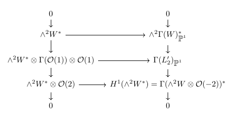
Figure 4.

where the left hand column is the Euler sequence on $\mbox{$\mathbb{P}$}^{1}$ twisted by $\wedge^{2}W^{*}\otimes\mathcal{O}(1)$, the right hand column comes from (18) and the map $\wedge^{2}W^{*}\rightarrow\wedge^{2}\Gamma(W)^{*}$ is the natural one. This diagram is $Sl_{2}(\mbox{$\mathbb{C}$})$ equivariant, where $Sl_{2}(\mbox{$\mathbb{C}$})$ acts on $\mbox{$\mathbb{P}$}^{1}$ in the usual way and on $\mbox{$\mathbb{P}$}^{1}\times\mbox{$\mathbb{P}$}^{1}$ by the diagonal action. In particular the morphism $\wedge^{2}W^{*}\otimes\mathcal{O}(2)\rightarrow\Gamma(\wedge^{2}W\otimes\mathcal{O}(-2))^{*}$ is $Sl_{2}(\mbox{$\mathbb{C}$})$ equivariant, by Lemma(4.2), it defines an embedding of $\mbox{$\mathbb{P}$}^{1}$ into $\mbox{$\mathbb{P}$}(\Gamma(\wedge^{2}W\otimes\mathcal{O}(-2))^{*})$ as a rational normal curve of degree $d-g-3$ .

Lemma 4.2.

[HPR92] Diagram in figure (4) gives rise to a commutative and exact diagram

Proposition 4.3.

$\Gamma(\wedge^{2}E)$ is generated by locally decomposable sections.

Proof: We have constructed maps $p_{2}^{*}(\wedge^{2}W^{*})\otimes\mathcal{O}(\Gamma)\rightarrow p_{1}^{*}(\wedge^{2}E)$ on $C\times\mbox{$\mathbb{P}$}^{1}$ and $q_{2}^{*}\wedge^{2}W^{*}\otimes\mathcal{O}(\bigtriangleup)\rightarrow q_{1}^{*}L_{2}^{\prime}$ on $\mbox{$\mathbb{P}$}^{1}\times\mbox{$\mathbb{P}$}^{1}$. Consider the diagram

Pulling the morphism $q_{2}^{*}\wedge^{2}W^{*}\otimes\mathcal{O}(\bigtriangleup)\rightarrow q_{1}^{*}L_{2}^{\prime}$ on $\mbox{$\mathbb{P}$}^{1}\times\mbox{$\mathbb{P}$}^{1}$ back to $C\times\mbox{$\mathbb{P}$}^{1}$, we get a morphism $p_{2}^{*}(\wedge^{2}W^{*})\otimes\mathcal{O}(\Gamma)\rightarrow p_{1}^{*}(\pi^{*}L_{2}^{\prime})$. By construction the diagram

commutes where the map $p_{1}^{*}(\pi^{*}L_{2}^{\prime})\rightarrow p_{1}^{*}\wedge^{2}E$ is the pullback via $p_{1}$ of the corresponding map in diagram in figure (3).Pushing this down via $\pi\times id$ to $\mbox{$\mathbb{P}$}^{1}\times\mbox{$\mathbb{P}$}^{1}$ leads to the commutative diagram

Now taking $q_{2*}$ of the outermost square we get

where the right hand vertical map is an isomorphism from Proposition 4.3.
Thus in order to compute the diagram

we can compute

and the result follows from Lemma 4.2. ∎

5. proof of main result

Here we want to prove Theorem 1.
We shall first show that for $2\leq i\leq d-g$, there is a natural epimorphism

$$\wedge^{i-2}\Gamma(W)^{*}\otimes\Gamma(L_{2}^{\prime})_{\mbox{$\mathbb{P}$}^{1}}\rightarrow\Gamma(L_{i}^{\prime})_{\mbox{$\mathbb{P}$}^{1}}\rightarrow 0$$

Setting $i=2$ in (14), we get

$$0\rightarrow\wedge^{2}W^{*}\rightarrow\wedge^{2}\Gamma(L)^{*}_{\mbox{$\mathbb{P}$}^{1}}\rightarrow L_{2}^{\prime}\rightarrow 0$$

Twisting with $\wedge^{i-2}\Gamma(W)^{*}$, we get an exact sequence

$$0\rightarrow\wedge^{i-2}\Gamma(W)^{*}\otimes\wedge^{2}W^{*}\rightarrow\wedge^{i-2}\Gamma(W)^{*}\otimes\wedge^{2}\Gamma(W)^{*}\rightarrow\wedge^{i-2}\Gamma(W)^{*}\otimes L_{2}^{\prime}\rightarrow 0$$

(since $\Gamma(L)\cong\Gamma(W)$) Combining this with (14), we get a diagram

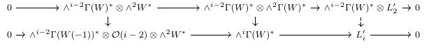
Figure 5.

Here the middle vertical map is the canonical one and the left hand vertical map is given by taking $\wedge^{i-2}$ of the dual evaluation sequence

$$0\rightarrow W^{*}\rightarrow\Gamma(W)^{*}\otimes\mathcal{O}_{\mbox{$\mathbb{P}$}^{1}}\rightarrow\Gamma(W(-1))^{*}\otimes\mathcal{O}_{\mbox{$\mathbb{P}$}^{1}}(1)\rightarrow 0$$

Taking $\wedge^{i-2}$ of the above sequence, we get

$$0\rightarrow\wedge^{2}W^{*}\otimes\wedge^{i-2}\Gamma(W(-1))^{*}\otimes\mathcal{O}_{\mbox{$\mathbb{P}$}^{1}}(i-2)\rightarrow\wedge^{i-2}\Gamma(W)^{*}\rightarrow F_{i-2}\rightarrow 0$$

$$0\rightarrow F_{i-2}\rightarrow\wedge^{i-2}\Gamma(W)^{*}\otimes\mathcal{O}_{\mbox{$\mathbb{P}$}^{1}}\rightarrow\wedge^{i-2}\Gamma(W(-1))^{*}\otimes\mathcal{O}_{\mbox{$\mathbb{P}$}^{1}}(i-2)\rightarrow 0$$

Tensoring above sequence with $\wedge^{2}W^{*}$, we get

$$0\rightarrow F_{i-2}\otimes\wedge^{2}W^{*}\rightarrow\wedge^{i-2}\Gamma(W)^{*}\otimes\mathcal{O}_{\mbox{$\mathbb{P}$}^{1}}\otimes\wedge^{2}W^{*}\rightarrow\wedge^{i-2}\Gamma(W(-1))^{*}\otimes\mathcal{O}_{\mbox{$\mathbb{P}$}^{1}}(i-2)\otimes\wedge^{2}W^{*}\rightarrow 0$$

Taking the associated cohomology sequence of commutative diagram in figure (5), we get the following commutative diagram:

Here $W$ is a rank $2$ vector bundle on $\mbox{$\mathbb{P}$}^{1}$ of degree $d-g-1$.

$$detW \cong \mathcal{O}(d-g-1)$$

$$detW^{*} \cong \mathcal{O}(-d+g+1)$$

$$i.e.\wedge^{2}W^{*} \cong \mathcal{O}(-d+g+1)$$

Since $2\leq d-g-1$
Thus $\Gamma(\wedge^{2}W)=0$

The top horizontal map is clearly surjective. The bottom horizontal map is surjective since $H^{2}$ vanishes on $\mbox{$\mathbb{P}$}^{1}$. By standard diagram chasing the middle horizontal map must be surjective thus giving our first claim.
By construction the natural diagram

Since $\Gamma(W)^{*}\cong\Gamma(L)^{*}$ and $\Gamma(L)^{*}$ can be identified with $\Gamma(E)$. By proposition (4.3), the horizontal maps are isomorphisms. Hence the natural map $\wedge^{i-2}\Gamma(E)\otimes\Gamma(\wedge^{2}E)\rightarrow\Gamma(\wedge^{i}E)$ is surjective and our claim follows from Proposition (4.3).

References

• [BE75] DavidΒ A. Buchsbaum and David Eisenbud, Generic free resolutions and a family of generically perfect ideals, Advances in Math. 18 (1975), no.Β 3, 245–301. MR 0396528
• [Eis05] David Eisenbud, The geometry of syzygies, Graduate Texts in Mathematics, vol. 229, Springer-Verlag, New York, 2005, A second course in commutative algebra and algebraic geometry. MR 2103875
• [ES12] Friedrich Eusen and Frank-Olaf Schreyer, A remark on a conjecture of Paranjape and Ramanan, Geometry and arithmetic, EMS Ser. Congr. Rep., Eur. Math. Soc., ZΓΌrich, 2012, pp.Β 113–123. MR 2987656
• [Gre84] MarkΒ L. Green, Koszul cohomology and the geometry of projective varieties, J. Differential Geom. 19 (1984), no.Β 1, 125–171. MR 739785 (85e:14022)
• [HPR92] K.Β Hulek, K.Β Paranjape, and S.Β Ramanan, On a conjecture on canonical curves, J. Algebraic Geom. 1 (1992), no.Β 3, 335–359. MR 1158621 (93c:14029)
• [PR88] Kapil Paranjape and S.Β Ramanan, On the canonical ring of a curve, Algebraic geometry and commutative algebra, Vol.Β II, Kinokuniya, Tokyo, 1988, pp.Β 503–516. MR 977775 (90b:14024)
• [Sch86] Frank-Olaf Schreyer, Syzygies of canonical curves and special linear series, Math. Ann. 275 (1986), no.Β 1, 105–137. MR 849058