Cholesky factorisation of linear systems coming from finite difference approximations of singularly perturbed problems

Abstract

We consider the solution of large linear systems of equations that arise when two-dimensional singularly perturbed reaction-diffusion equations are discretized. Standard methods for these problems, such as central finite differences, lead to system matrices that are positive definite. The direct solvers of choice for such systems are based on Cholesky factorisation. However, as observed in [6], these solvers may exhibit poor performance for singularly perturbed problems. We provide an analysis of the distribution of entries in the factors based on their magnitude that explains this phenomenon, and give bounds on the ranges of the perturbation and discretization parameters where poor performance is to be expected.

Keywords: Cholesky factorization, Shishkin mesh, singularly perturbed.

1 Introduction

We consider the singularly perturbed two dimensional reaction-diffusion problem:

$$-\varepsilon^{2}\Delta u+b(x,y)u=f(x,y),\quad\Omega=(0,1)^{2},\quad u(\partial\Omega)=g(x,y),$$ (1)

where the “perturbation parameter”, $\varepsilon$, is a small and positive, and the functions $g$, $b$ and $f$ are given, with $b(x,y)\geq\beta^{2}>0$.

We are interested in the numerical solution of (1) by the following standard finite difference technique. Denote the mesh points of an arbitrary rectangular mesh as $(x_{i},y_{j})$ for $i,j\in\{0,1,\dots,N\}$, write the local mesh widths as $h_{i}=x_{i}-x_{i-1}$ and $k_{j}=y_{j}-y_{j-1}$, and let $\bar{h}_{i}=(x_{i+1}-x_{i-1})/2$, and $\bar{k}_{j}=(y_{j+1}-y_{j-1})/2$. Then the linear system for the finite difference method can be written as

$$AU^{N}=f^{N},\quad\text{ where }\quad A=\left(-\varepsilon^{2}\Delta^{N}+\bar{h}_{i}\bar{k}_{j}b(x_{i},y_{j})\right),$$ (2a)

and $$\Delta^{N}$$ is the symmetrised 5-point second order central difference operator

$$\Delta^{N}:=\left(\begin{matrix}&\dfrac{\bar{h}_{i}}{k_{j+1}}&\\ \dfrac{\bar{k}_{j}}{h_{i}}&-\left(\bar{k}_{j}\left(\dfrac{1}{h_{i}}+\dfrac{1}{h_{i+1}}\right)+\bar{h}_{i}\left(\dfrac{1}{k_{j}}+\dfrac{1}{k_{j+1}}\right)\right)&\dfrac{\bar{k}_{j}}{h_{i+1}}\\ &\dfrac{\bar{h}_{i}}{k_{j}}&\end{matrix}\right).$$ (2b)

It is known that the scheme (2) applied to (1) on a boundary layer-adapted mesh with $N$ intervals in each direction yields a parameter robust approximation, see, e.g., [2, 5]. Since $A$ in (2a) is a banded, symmetric and positive definite, the direct solvers of choice are variants on Cholesky factorisation. This is based on the idea that there exists a unique lower-triangular matrix $L$ (the “Cholesky factor”) such that $A=LL^{T}$ (see, e.g., [4, Thm. 4.25]). Conventional wisdom is that the computational complexity of these methods depends exclusively on $N$ and the structure of the matrix (i.e., its sparsity pattern). However, MacLachlan and Madden [6, §4.1] observe that standard implementations of Cholesky factorisation applied to (2a) perform poorly when $\varepsilon$ in (1) is small. Their explanation is that the Cholesky factor, $L$, contains many small entries that fall in to the range of subnormal floating-point numbers. These are numbers that have magnitude (in exact arithmetic) between $2^{-1074}\approx 5\times 10^{-324}$ and $2^{-1022}\approx 2\times 10^{-308}$ (called realmin in MATLAB). Numbers greater than $2.2\times 10^{-308}$ are represented faithfully in IEEE standard double precision, while numbers less than $2^{-1074}$ are flushed to zero (we’ll call such numbers “underflow-zeros”). Floats between these values do not have full precision, but allow for “gradual underflow”, which (ostensibly) leads to more reliable computing (see, e.g., [7, Chap. 7]). Unlike standard floating-point numbers, most CPUs do not support operations on subnormals directly, but rely on microcode implementations, which are far less efficient. Thus it is to be expected that it is more time-consuming to factorise $A$ in (2a) when $\varepsilon$ is small. As an example of this, consider (2) where $N=128$ and the mesh is uniform. The nonzero entries of the associated Cholesky factor are located on the diagonals that are at most a distance $N$ from main diagonal. In Figure 1, we plot the absolute value of largest entry of a given diagonal of $L$, as a function of its distance from the main diagonal. On the left of Figure 1, where $\varepsilon=1$, we observe that the magnitude of the largest entry gradually decays away from the location of the nonzero entries of $A$. In contrast, when $\varepsilon=10^{-6}$ (on the right), magnitude of the largest entry decays exponentially.

To demonstrate the effect of this on computational efficiency, in Table 1 we show the time, in seconds, taken to compute the factorisation of $A$ in (2a) with a uniform mesh, and $N=512$, on a single core of AMD Opteron 2427, 2200 MHz processor, using CHOLMOD [1] with “natural order” (i.e., without a fill reducing ordering). Observe that the time-to-factorisation increases from 52 seconds when $\varepsilon$ is large, to nearly 500 seconds when $\varepsilon=10^{-3}$, when over 1% of the entries are in the subnormal range. When $\varepsilon$ is smaller again, the number of nonzero entries in $L$ is further reduced, and so the execution time decreases as well.

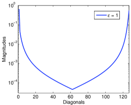
Figure 1: Semi-log plot of maximal entries on diagonals of $L$ with $N=128$, and $\varepsilon=1$ (left) and $\varepsilon=10^{-6}$ (right).

$\varepsilon$	$10^{-1}$	$10^{-2}$	$10^{-3}$	$10^{-4}$	$10^{-5}$	$10^{-6}$
Time (s)	52.587	52.633	496.887	175.783	74.547	45.773
Nonzeros in $L$	133,433,341	133,433,341	128,986,606	56,259,631	33,346,351	23,632,381
Subnormals in $L$	0	0	1,873,840	2,399,040	1,360,170	948,600
Underflow zeros	0	0	4,446,735	77,173,710	100,086,990	109,800,960

Table 1: Time taken (in seconds) to compute the Cholesky factor, $L$, of $A$ in (2) on a uniform mesh with $N=512$. The number of nonzeros, subnormals, and underflow-zeros in $L$ are also shown.

Our goal is to give an analysis that fully explains the observations of Figure 1 and Table 1, and that can also be exploited in other solver strategies. We derive expressions, in terms of $N$ and $\varepsilon$, for the magnitude of entries of $L$ as determined by their location. Ultimately, we are interested in the analysis of systems that arise from the numerical solution of (1) on appropriate boundary layer-adapted meshes. Away from the boundary, such meshes are usually uniform. Therefore, we begin in Section 2.1 with studying a uniform mesh discretisation, in the setting of exact arithmetic, which provides mathematical justification for observations in Figure 1. In Section 2.2, this analysis is used to quantify to number of entries in the Cholesky factors of a given magnitude. As an application of this, we show how to determine the number of subnormal numbers that will occur in $L$ in a floating-point setting, and also determine an lower bound for $\varepsilon$ for which the factors are free of subnormal numbers. Finally, the Cholesky factorisation on a boundary layer-adapted mesh is discussed in Section 2.3, and our conclusions are summarised in Section 3.

2 Cholesky factorisation on a uniform mesh

2.1 The magnitude of the fill-in entries

We consider the discretisation (2b) of the model problem (1) on a uniform mesh with $N$ intervals on each direction. The equally spaced stepsize is denoted by $h=N^{-1}$. When $\varepsilon\ll h$, which is typical in a singularly perturbed regime, the system matrix in (2a) can be written as the following 5-point stencil

$$A=\begin{pmatrix}&-\varepsilon^{2}&\\ -\varepsilon^{2}\ &4\varepsilon^{2}+h^{2}b(x_{i},y_{j})\ &-\varepsilon^{2}\\ &-\varepsilon^{2}&\end{pmatrix}=\begin{pmatrix}&-\varepsilon^{2}&\\ -\varepsilon^{2}\ &\mathcal{O}{(h^{2})}\ &-\varepsilon^{2}\\ &-\varepsilon^{2}&\end{pmatrix},$$ (3)

since $(4\varepsilon^{2}+h^{2}b(x_{i},y_{j}))=\mathcal{O}(h^{2})$, where we write $f(\cdot)=\mathcal{O}{(g(\cdot))}$ if there exist positive constants $C_{0}$ and $C_{1}$, independent of $N$ and $\varepsilon$, such that $C_{0}|g(\cdot)|\leq~{}f(\cdot)\leq~{}C_{1}|g(\cdot)|$.

Algorithm 1 presents a version of Cholesky factorisation which adapted from [4, page 143]. It computes a lower triangular matrix $L$ such that $A=LL^{T}$. We will follow MATLAB notation by denoting $A=[a(i,j)]$ and $L=[l(i,j)]$.

Algorithm 1 Cholesky factorisation:

for $j=1:n$
classif $j=1$
classclasscfor $i=j:n$
classclassclass$l(i,j)=\dfrac{a(i,j)}{\sqrt{a(j,j)}}$
classclassend
classelseif $(j>1)$
classclasscfor $i=j:n$
classclassclass$l(i,j)=\dfrac{a(i,j)-\sum_{k=1}^{j-1}l(i,k)l(j,k)}{\sqrt{a(j,j)}}$
classclassend
classend
end

We set $m=N-1$, so $A$ is a sparse, banded $m^{2}\times m^{2}$ matrix, with a bandwidth of $m$, and has no more than five nonzero entries per row. Its factor, $L$, is far less sparse: although it has the same bandwidth as $A$, it has $\mathcal{O}(m)$ nonzeros per row (see, e.g., [3, Prop. 2.4]). The set of non-zero entries in $L$ that are zero in the corresponding location in $A$ is called the fill-in. We want to find a recursive way to express the magnitude of these fill-in entries, in terms of $\varepsilon$ and $h$.

To analyse the magnitude of the fill-in entries, we borrow notation from [8, Sec. 10.3.3], and form distinct sets denoted $L^{[0]}$, $L^{[1]},\dots,L^{[m]}$ where all entries of $L$ of the same magnitude (in a sense explained carefully below) belong to the same set. We denote by $l^{[k]}$ the magnitude of entries in $L^{[k]}$, i.e., $l(i,j)\in L^{[k]}$ if and only if $l(i,j)$ is $\mathcal{O}(l^{[k]})$. We shall see that these sets are quite distinct, meaning that $l^{[k]}\gg l^{[k+1]}$ for $k\geq 1$. $L^{[0]}$ is used to denote the set of nonzero entries in $A$, and entries of $L$ that are zero (in exact arithmetic) are defined to belong to $L^{[\infty]}$.

In Algorithm 1, all the entries of $L$ are initialised as zero, and so belong to $L^{[\infty]}$. Suppose that $p_{i,j}$ is such that $l(i,j)\in L^{[p_{i,j}]}$, so, initially, each $p_{i,j}=\infty$. At each sweep through the algorithm, a new value of $l(i,j)$ is computed, and so $p_{i,j}$ is modified. From line 8 in Algorithm 1, we can see that the $p_{i,j}$ is updated by

$$p_{i,j}=\begin{cases}\min\{0,p_{i,1}+p_{j,1}+1,p_{i,2}+p_{j,2}+1,\ldots,p_{i,j-1}+p_{j,j-1}+1\},\ \textrm{if }\ a(i,j)\neq 0,\\ \min\{p_{i,1}+p_{j,1}+1,p_{i,2}+p_{j,2}+1,\ldots,p_{i,j-1}+p_{j,j-1}+1\},\ \textrm{otherwise}.\end{cases}$$

Then, as we shall explain in detail below, it can be determined that $L$ has a block structure shown in (4a)–(4c), where, for brevity, the entries belonging to $L^{[k]}$ are denoted by $[k]$, and the entries that corresponding to nonzero entries of original matrix are written in terms of their magnitude:

$$L=\begin{pmatrix}M&&&&\\ P&Q&&&\\ &P&Q&&\\ &&\ddots&\ddots&\\ &&&P&Q\\ \end{pmatrix},\text{ where }M=\begin{pmatrix}\mathcal{O}{(h)}&&&&\\ \mathcal{O}{(\varepsilon^{2}/h)}&\mathcal{O}{(h)}&&&\\ &\mathcal{O}{(\varepsilon^{2}/h)}&\mathcal{O}{(h)}&&\\ &&\ddots&\ddots&\\ &&&\mathcal{O}{(\varepsilon^{2}/h)}&\mathcal{O}{(h)}\\ \end{pmatrix},$$ (4a)

$$P=\begin{pmatrix}\mathcal{O}{(\varepsilon^{2}/h)}&[1]&[2]&[3]&\ldots&[m-2]&[m-1]\\ &\mathcal{O}{(\varepsilon^{2}/h)}&[1]&[2]&\ldots&[m-3]&[m-2]\\ &&\ddots&\ddots&\ddots&\vdots&\vdots\\ &&&\mathcal{O}{(\varepsilon^{2}/h)}&[1]&[2]&[3]\\ &&&&\mathcal{O}{(\varepsilon^{2}/h)}&[1]&[2]\\ &&&&&\mathcal{O}{(\varepsilon^{2}/h)}&[1]\\ &&&&&&\mathcal{O}{(\varepsilon^{2}/h)}\\ \end{pmatrix},$$ (4b)

$$Q=\begin{pmatrix}\mathcal{O}{(h)}&&&&&&\\ \mathcal{O}{(\varepsilon^{2}/h)}&\mathcal{O}{(h)}&&&&&\\ [3]&\mathcal{O}{(\varepsilon^{2}/h)}&\mathcal{O}{(h)}&&&&\\ [4]&[3]&\mathcal{O}{(\varepsilon^{2}/h)}&\mathcal{O}{(h)}&&&\\ \vdots&\vdots&\ddots&\ddots&\ddots&&\\ [m-1]&[m-2]&\ldots&[3]&\mathcal{O}{(\varepsilon^{2}/h)}&\mathcal{O}{(h)}&\\ [m]&[m-1]&\ldots&[4]&[3]&\mathcal{O}{(\varepsilon^{2}/h)}&\mathcal{O}{(h)}\\ \end{pmatrix}.$$ (4c)

We now explain why the entries of $L$, which are computed by column, have the structure shown in (4). According to Algorithm 1, the first column of $L$ is computed by $l(i,1)=a(i,1)/\sqrt{a(1,1)}$, which shows that there is no fill-in entry in this column. For the second column, the only fill-in entry is

$$l(m+1,2)=\frac{a(m+1,2)-l(m+1,1)l(2,1)}{\sqrt{a(2,2)}}=\frac{0-\mathcal{O}{(\varepsilon^{2}/h)}\mathcal{O}{(\varepsilon^{2}/h)}}{\mathcal{O}{(h)}}=\mathcal{O}{(\varepsilon^{4}/h^{3})},$$

where $l(m+1,1)$ and $l(2,1)$ belong to $L^{[0]}$, so $l(m+1,2)$ is in $L^{[1]}$. Similarly, there are two fill-ins in third column: $l(m+1,3)$ and $l(m+2,3)$. The entry $l(m+1,3)$ is computed as

$$\begin{split}l(m+1,3)&=\frac{a(m+1,3)-\sum_{k=1}^{2}l(m+1,k)l(3,k)}{\sqrt{a(3,3)}}=\frac{-l(m+1,2)l(3,2)}{\sqrt{a(3,3)}}\end{split}$$

which is $\mathcal{O}{(\varepsilon^{6}/h^{5})}$; moreover, since $l(m+1,2)\in L^{[1]}$, and $l(3,2)\in L^{[0]}$, so $l(m+1,3)\in L^{[2]}$. Similarly, it is easy to see that $l(m+2,3)\in L^{[1]}$. We may now proceed by induction to show that $l(m+1,j+1)=\mathcal{O}{(\varepsilon^{2(j+1)}/h^{(2j+1)})}$ belongs to $L^{[j]}$, for $1\leq j\leq m-2$. Suppose $l(m+1,j)=\mathcal{O}{(\varepsilon^{(2j)}/h^{(2j-1)})}\in L^{[j-1]}$. Then

$$\begin{split}l(m+1,j+1)&=\frac{a(m+1,j+1)-\sum_{k=1}^{j}l(m+1,k)l(j+1,k)}{\sqrt{a(j,j)}}\\ &=\frac{-l(m+1,j)l(j+1,j)}{\sqrt{a(j,j)}},\quad\textrm{since }l(j+1,k)=0,\quad\forall k\leq j-1,\\ &=\frac{\mathcal{O}{(\varepsilon^{(2j)}/h^{(2j-1)})}\mathcal{O}{(\varepsilon^{2}/h)}}{\mathcal{O}{(h)}}=\mathcal{O}{(\varepsilon^{(2j+2)}/h^{(2j+1)})}.\\ \end{split}$$

And, because $l(j+1,j)\in L^{[0]}$, we can deduce that $l(m+1,j+1)\in L^{[j]}$. The process is repeated from column 1 to column $m$, yielding the pattern for $P$ shown in (4b).

A similar process is used to show that $Q$ is as given in (4c). Its first fill-in entry is $l(m+3,m+1)$. Note that $a(m+3,m+1)=l(m+1,1)=l(m+1,2)=0$, that the magnitude of the entry in $L^{[j]}$ is $\mathcal{O}{(\varepsilon^{2(j+1)}/h^{(2j+1)})}$, and that the sum of two entries of the different magnitude has the same magnitude as larger one. Then

$$\begin{split}l(m+3,m+1)&=\frac{-\sum_{k=3}^{m}l(m+3,k)l(m+1,k)}{\sqrt{a(m+1,m+1)}}\\ &=\left[\mathcal{O}{\left(\frac{\varepsilon^{2}}{h}\right)}\mathcal{O}{\left(\frac{\varepsilon^{6}}{h^{5}}\right)}+\mathcal{O}{\left(\frac{\varepsilon^{4}}{h^{3}}\right)}\mathcal{O}{\left(\frac{\varepsilon^{8}}{h^{7}}\right)}+\ldots\right.\\ &\qquad\left.\,\,+\mathcal{O}{\left(\frac{\varepsilon^{2(m-2)}}{h^{(2(m-3)+1)}}\right)}\mathcal{O}{\left(\frac{\varepsilon^{2(m)}}{h^{(2(m-1)+1)}}\right)}\right]\frac{1}{\mathcal{O}{(h)}}\\ &=\left[\mathcal{O}{\left(\frac{\varepsilon^{2}}{h}\right)}\mathcal{O}{\left(\frac{\varepsilon^{6}}{h^{5}}\right)}\right]\frac{1}{\mathcal{O}{(h)}}=\mathcal{O}\left(\frac{\varepsilon^{8}}{h^{7}}\right),\end{split}$$

and so $l(m+3,m+1)$ belongs to $L^{[3]}$. Proceeding inductively, as was done for $P$ shows that $Q$ has the form given in (4c). Furthermore, the same process applies to each block of $L$ in (4a). Summarizing, we have established the following result.

Theorem 1.

The fill-in entries of the Cholesky factor $L$ of the matrix $A$ defined in (3) is as given in (4). Moreover, setting $\delta=\varepsilon/h$, the magnitude $l^{[k]}$ is

$$l^{[k]}=\mathcal{O}{\left(\varepsilon^{2(k+1)}/h^{(2k+1)}\right)}=\mathcal{O}{\left(\delta^{2(k+1)}h\right)}\quad\text{ for }\quad k=1,2,\dots,m.$$ (5)

2.2 Distribution of fill-in entries in a floating-point setting

In practice, Cholesky factorisation is computed in a floating-point setting. As discussed in Section 1, the time taken to compute these factorisations increases greatly if there are many subnormal numbers present. Moreover, even the underflow-zeros in the factors can be expensive to compute, since they typically arise from intermediate calculations involving subnormal numbers. Therefore, in this section we use the analysis of Section 2.1, to estimate, in terms of $\varepsilon$ and $N$, the number of entries in $L$ that are of a given magnitude. From this, one can easily predict the number of subnormals and underflow-zeros in $L$.

Lemma 1.

Let $A$ be the $m^{2}\times m^{2}$ matrix in (2) where the mesh is uniform. Then the number of nonzero entries in the Cholesky factor $L$ (i.e., $A=LL^{T}$) computed using exact arithmetic is

$$L_{nz}=m^{3}+m-1.$$ (6)

Proof.

Since $A$ has bandwidth $m$, and so too does $L$ ([3, Prop. 2.3]). By the Algorithm 1, the fill-in entries only occur from row $(m+1)$. So, from row $(m+1)$, any row of $L$ has $(m+1)$ nonzero entries and there are $m(m-1)$ such rows, plus $2m-1$ nonzero entries from top-left block $M$ in (4a). Summing these values, we obtain (6). ∎

Let $|L^{[k]}|$ be the number of fill-in entries which belong to $L^{[k]}$. To estimate $|L^{[k]}|$, it is sufficient to evaluate the fill-in entries in the submatrices $P$ and $Q$ shown in (4). Table 2 describes the number of fill-in entries associated with their magnitude.

$L^{[k]}$	$|L^{[k]}|$ in $P$	$|L^{[k]}|$ in $Q$	$|L^{[k]}|$ in $[P,Q]$
$L^{[1]}$	$m-1$	0	$m-1$
$L^{[2]}$	$m-2$	0	$m-2$
$L^{[3]}$	$m-3$	$m-2$	$2m-5$
⋮	⋮	⋮	⋮
$L^{[k]}$	$m-k$	$m-k+1$	$2m-2k+1$
⋮	⋮	⋮	⋮
$L^{[m-2]}$	2	$3$	5
$L^{[m-1]}$	1	$2$	3
$L^{[m]}$	0	1	1

Table 2: Number of fill-in entries in $P$ and $Q$ associated with their magnitude.

Note that there are $(m-1)$ blocks like $[P,Q]$ in $L$. Then, since $l^{[k]}\ll l^{[k-1]}$, and the smallest (exact) nonzero entries belong to $L^{[m]}$ we can use Table 2 to determine the number of entries that are at most $\mathcal{O}(l^{[p]})$, for some given $p$ as:

$$\sum\limits_{k=p}^{m}|L^{[k]}|=\begin{cases}(m-1)(2m-3)+(m-1)(m-2)^{2}=(m-1)^{3}&p=1,\\ (m-1)(m-2)+(m-1)(m-2)^{2}=(m-2)(m-1)^{2}&p=2,\\ (m-1)(m-p+1)^{2}&p\geq 3.\end{cases}$$

These equations can be combined and summarised as follows.

Theorem 2.

Let $A$ be the matrix of the form (3). Then, the number of fill-in entries associated with their magnitude of the matrix $L$ satisfies

$$\sum\limits_{k=p}^{m}|L^{[k]}|\leq(m-1)(m-p+1)^{2},\quad p\geq 1.$$ (7)

Combining Theorems 1 and 2 enables us to accurately predict the total number, and location, of subnormal and underflow-zero entries in $L$, for given $N$ and $\varepsilon$. For example, recall Figure 1 where we took $\varepsilon=10^{-6}$ and $N=128$. To determine, using Theorem 1, the diagonals where entries are subnormal, we solve

$$(\varepsilon N)^{2(k+1)}=2^{-1022}N,$$ (8)

for $N=128$ and $\varepsilon=10^{-6}$, which yields $k\approx 38$. It clearly agrees with the observation in Figure 1; i.e., the maximal value of the entries on diagonals 38 and $N-38=90$ are less than realmin. Similarly, all entries on diagonals between 40 and 88 are flushed to zero.

As a further example, letting $N=512$ and $\varepsilon=10^{-6}$, by (7), the total number of underflow-zero and subnormal entries in $L$ are, respectively,

$$\quad\sum\limits_{k=48}^{511}|L^{[k]}|=109,800,960,~{}\text{ and }~{}\sum\limits_{k=46}^{47}|L^{[k]}|=\sum\limits_{k=46}^{511}|L^{[k]}|-\sum\limits_{k=48}^{511}|L^{[k]}|=948,600.$$

This is exactly what is observed in Table 1. Moreover, the total number of entries with magnitude less than realmin is 110,749,560 which is over 80% of the exact nonzero entries (cf. Lemma 1) in $L$: 133,433,341. Such a predictable appearance of subnormals and underflows is important in the sense of choosing suitable linear solvers, i.e., direct or iterative ones.

More generally, we can use (8) to investigate ranges of $N$ and $\varepsilon$ for which subnormal entries occur (assuming $\varepsilon\leq N^{-1}$). Since the largest possible value of $k$ is $m$, a Cholesky factor will have subnormal entries if $\varepsilon$ and $N$ are such that $(\varepsilon N)^{2N}\leq 2^{-1022}N$. Rearranging, this gives that

$$\varepsilon\leq\frac{1}{N}\left(2^{-1022}N\right)^{1/(2N)}=2^{-511/N}N^{(1/(2N)-1)}=:g(N).$$ (9)

The function $g$ defined in (9) is informative because it gives the largest value of $\varepsilon$ for a discretisation with given $N$ leads to a Cholesky factor with entries less than $2^{-1022}$. For example, Figure 2 (on the left) shows $g(N)$ for $N\in[200,500]$. It demonstrates that, for $\varepsilon\leq 1.05\times 10^{-3}$ (determined numerically), subnormal entries are to be expected for some values of $N$ (cf. Table 1). The line $\varepsilon=10^{-3}$ intersects $g$ at approximately $N=263$ and $N=484$, meaning that a discretisation with $263\leq N\leq 484$ yields entries with the magnitude less than $2^{-1022}$ in $L$ for $\varepsilon=10^{-3}$. On the right of Figure 2 we show that, for large $N$, $g(N)$ decays like $N^{-1}$. Since we are interested in the regime where $\varepsilon\leq N^{-1}$, this shows that, for small $\varepsilon$, subnormals are to be expected for all but the smallest values of $N$.

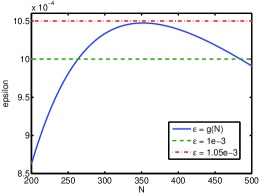
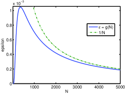
Figure 2: The function $g(N)$ defined in (9) with $N\in[200,500]$ (left) and $N\in[1,5000]$ (right).

2.3 Boundary layer-adapted meshes

Our analysis so far has been for computations on uniform meshes. However, a scheme such as (2) for (1) is usually applied on a layer-adapted mesh, such as a Shishkin mesh. For these meshes, in the neighbourhood of the boundaries, and especially near corner layers, the local mesh width is $\mathcal{O}(\varepsilon N^{-1})$ in each direction, and so the entries of the system matrix are of the same order, and no issue with subnormal numbers is likely to arise. However, away from layers, these fitted meshes are usually uniform, with a local mesh width of $\mathcal{O}(N^{-1})$, and so the analysis outlined above applies directly. Since roughly one quarter (depending on mesh construction) of all mesh points are located in this region, the influence on the computation is likely to be substantial.

The main complication in extending our analysis to, say, a Shishkin mesh, is in considering the “edge layers”, where the mesh width may be $\mathcal{O}(\varepsilon N^{-1})$ in one coordinate direction, and $\mathcal{O}(N^{-1})$ in another. Although we have not analysed this situation carefully, in practise it seems that the factorisation behaves more like a uniform mesh. This is demonstrated in Table 3 below. Comparing with Table 1, we see, for small $\varepsilon$, the number of entries flushed to zero is roughly three-quarters that of the uniform mesh case.

$\varepsilon$	$10^{-1}$	$10^{-2}$	$10^{-3}$	$10^{-4}$	$10^{-5}$	$10^{-6}$
Time (s)	52.580	58.213	447.533	179.540	101.507	73.250
Nonzeros in $L$	133,433,341	133,240,632	127,533,193	78,091,189	62,082,599	54,497,790
Subnormals in $L$	0	28,282	2,648,308	1,669,345	1,079,992	814,291
Underflow zeros	0	192,709	5,900,148	55,342,152	71,350,742	78,935,551

Table 3: Time taken (in seconds) to compute the Cholesky factor, $L$, of $A$ in (2) on a Shishkin mesh with $N=512$. The number of nonzeros, subnormals, and underflow-zeros in $L$ are also shown.

3 Conclusions

The paper addresses, in a comprehensive way, issues raised in [6] by showing how to predict the number and location of subnormal and underflow entries in the Cholesky factors of $A$ in (2a) for given $\varepsilon$ and $N$.

Further developments on this work are possible. In particular, the analysis shows that, away from the existing diagonals, the magnitude of fill-in entries decay exponentially, as seen in (5), a fact that could be exploited in the design of preconditioners of iterative solvers. For example, as shown in Lemma 1, the Cholesky factor of $A$, in exact arithmetic, has $\mathcal{O}(N^{3})$ nonzero entries. However, Theorem 2 shows that, in practice (i.e., in a float-point setting), there are only $\mathcal{O}(N^{2})$ entries in $L$ when $\varepsilon$ is small and $N$ is large. This suggests that, for a singularly perturbed problem, an incomplete Cholesky factorisation may be a very good approximation for $L$. This is a topic of ongoing work.

In this paper we have restricted our study to Cholesky factorisation of the coefficient matrix arising from finite-difference discretisation of the model problem (1) on a uniform and a boundary layer-adapted mesh, the same phenomenon is also observed in more general context of singularly perturbed problems. That includes the $LU$-factorisations of the coefficient matrices coming from both finite difference and finite element methods applied to reaction-diffusion and convection-diffusion problems, though further investigation is required to establish the details.

References

- [1] Y. Chen, T.A. Davis, W.W. Hager, and S. Rajamanickam, Algorithm 887: CHOLMOD, supernodal sparse cholesky factorization and update/downdate, ACM Trans. Math. Softw., 35 (2008), pp. 22:1–22:14.
- [2] C. Clavero, J.L. Gracia, and E. O’Riordan. A parameter robust numerical method for a two dimensional reaction-diffusion problem. Math. Comput., 74(252):1743–1758, 2005.
- [3] James W. Demmel. Applied numerical linear algebra. Society for Industrial and Applied Mathematics (SIAM), Philadelphia, PA (1997).
- [4] Gene H. Golub and Charles F. Van Loan. Matrix computations. Johns Hopkins Studies in the Mathematical Sciences. Johns Hopkins University Press, Baltimore, MD, third edition (1996).
- [5] Torsten Linß. Layer-adapted meshes for reaction-convection-diffusion problems, volume 1985 of Lecture Notes in Mathematics. Springer-Verlag, Berlin, 2010.
- [6] S. MacLachlan and N. Madden, Robust solution of singularly perturbed problems using multigrid methods, SIAM J. Sci. Comput., 35 (2013), pp. A2225-A2254.
- [7] Michael L. Overton. Numerical computing with IEEE floating point arithmetic. Society for Industrial and Applied Mathematics (SIAM), Philadelphia, PA, 2001.
- [8] Saad, Y. Iterative methods for sparse linear systems, Society for Industrial and Applied Mathematics, Philadelphia, PA, second edition (2003).