A Simple Way to Initialize Recurrent Networks of Rectified Linear Units

Abstract

Learning long term dependencies in recurrent networks is difficult due to vanishing and exploding gradients. To overcome this difficulty, researchers have developed sophisticated optimization techniques and network architectures. In this paper, we propose a simpler solution that use recurrent neural networks composed of rectified linear units. Key to our solution is the use of the identity matrix or its scaled version to initialize the recurrent weight matrix. We find that our solution is comparable to a standard implementation of LSTMs on our four benchmarks: two toy problems involving long-range temporal structures, a large language modeling problem and a benchmark speech recognition problem.

1 Introduction

Recurrent neural networks (RNNs) are very powerful dynamical systems and they are the natural way of using neural networks to map an input sequence to an output sequence, as in speech recognition and machine translation, or to predict the next term in a sequence, as in language modeling. However, training RNNs by using back-propagation through time [30] to compute error-derivatives can be difficult. Early attempts suffered from vanishing and exploding gradients [15] and this meant that they had great difficulty learning long-term dependencies. Many different methods have been proposed for overcoming this difficulty.

A method that has produced some impressive results [23, 24] is to abandon stochastic gradient descent in favor of a much more sophisticated Hessian-Free (HF) optimization method. HF operates on large mini-batches and is able to detect promising directions in the weight-space that have very small gradients but even smaller curvature. Subsequent work, however, suggested that similar results could be achieved by using stochastic gradient descent with momentum provided the weights were initialized carefully [34] and large gradients were clipped [28]. Further developments of the HF approach look promising [35, 25] but are much harder to implement than popular simple methods such as stochastic gradient descent with momentum [34] or adaptive learning rates for each weight that depend on the history of its gradients [5, 14].

The most successful technique to date is the Long Short Term Memory (LSTM) Recurrent Neural Network which uses stochastic gradient descent, but changes the hidden units in such a way that the backpropagated gradients are much better behaved [16]. LSTM replaces logistic or tanh hidden units with “memory cells” that can store an analog value. Each memory cell has its own input and output gates that control when inputs are allowed to add to the stored analog value and when this value is allowed to influence the output. These gates are logistic units with their own learned weights on connections coming from the input and also the memory cells at the previous time-step. There is also a forget gate with learned weights that controls the rate at which the analog value stored in the memory cell decays. For periods when the input and output gates are off and the forget gate is not causing decay, a memory cell simply holds its value over time so the gradient of the error w.r.t. its stored value stays constant when backpropagated over those periods.

The first major success of LSTMs was for the task of unconstrained handwriting recognition [12]. Since then, they have achieved impressive results on many other tasks including speech recognition [13, 10], handwriting generation [8], sequence to sequence mapping [36], machine translation [22, 1], image captioning [38, 18], parsing [37] and predicting the outputs of simple computer programs [39].

The impressive results achieved using LSTMs make it important to discover which aspects of the rather complicated architecture are crucial for its success and which are mere passengers. It seems unlikely that Hochreiter and Schmidhuber’s [16] initial design combined with the subsequent introduction of forget gates [6, 7] is the optimal design: at the time, the important issue was to find any scheme that could learn long-range dependencies rather than to find the minimal or optimal scheme. One aim of this paper is to cast light on what aspects of the design are responsible for the success of LSTMs.

Recent research on deep feedforward networks has also produced some impressive results [19, 3] and there is now a consensus that for deep networks, rectified linear units (ReLUs) are easier to train than the logistic or tanh units that were used for many years [27, 40]. At first sight, ReLUs seem inappropriate for RNNs because they can have very large outputs so they might be expected to be far more likely to explode than units that have bounded values. A second aim of this paper is to explore whether ReLUs can be made to work well in RNNs and whether the ease of optimizing them in feedforward nets transfers to RNNs.

2 The initialization trick

In this paper, we demonstrate that, with the right initialization of the weights, RNNs composed of rectified linear units are relatively easy to train and are good at modeling long-range dependencies. The RNNs are trained by using backpropagation through time to get error-derivatives for the weights and by updating the weights after each small mini-batch of sequences. Their performance on test data is comparable with LSTMs, both for toy problems involving very long-range temporal structures and for real tasks like predicting the next word in a very large corpus of text.

We initialize the recurrent weight matrix to be the identity matrix and biases to be zero. This means that each new hidden state vector is obtained by simply copying the previous hidden vector then adding on the effect of the current inputs and replacing all negative states by zero. In the absence of input, an RNN that is composed of ReLUs and initialized with the identity matrix (which we call an IRNN) just stays in the same state indefinitely. The identity initialization has the very desirable property that when the error derivatives for the hidden units are backpropagated through time they remain constant provided no extra error-derivatives are added. This is the same behavior as LSTMs when their forget gates are set so that there is no decay and it makes it easy to learn very long-range temporal dependencies.

We also find that for tasks that exhibit less long range dependencies, scaling the identity matrix by a small scalar is an effective mechanism to forget long range effects. This is the same behavior as LTSMs when their forget gates are set so that the memory decays fast.

Our initialization scheme bears some resemblance to the idea of Mikolov et al. [26], where a part of the weight matrix is fixed to identity or approximate identity. The main difference of their work to ours is the fact that our network uses the rectified linear units and the identity matrix is only used for initialization. The scaled identity initialization was also proposed in Socher et al. [32] in the context of tree-structured networks but without the use of ReLUs. Our work is also related to the work of Saxe et al. [31], who study the use of orthogonal matrices as initialization in deep networks.

3 Overview of the experiments

Consider a recurrent net with two input units. At each time step, the first input unit has a real value and the second input unit has a value of 0 or 1 as shown in figure 1. The task is to report the sum of the two real values that are marked by having a 1 as the second input [16, 15, 24]. IRNNs can learn to handle sequences with a length of 300, which is a challenging regime for other algorithms.

Another challenging toy problem is to learn to classify the MNIST digits when the 784 pixels are presented sequentially to the recurrent net. Again, the IRNN was better than the LSTM, having been able to achieve 3% test set error compared to 34% for LSTM.

While it is possible that a better tuned LSTM (with a different architecture or the size of the hidden state) would outperform the IRNN for the above two tasks, the fact that the IRNN performs as well as it does, with so little tuning, is very encouraging, especially given how much simpler the model is, compared to the LSTM.

We also compared IRNNs with LSTMs on a large language modeling task. Each memory cell of an LSTM is considerably more complicated than a rectified linear unit and has many more parameters, so it is not entirely obvious what to compare. We tried to balance for both the number of parameters and the complexity of the architecture by comparing an LSTM with N memory cells with an IRNN with four layers of N hidden units, and an IRNN with one layer and 2N hidden units. Here we find that the IRNN gives results comparable to the equivalent LSTM.

Finally, we benchmarked IRNNs and LSTMs on a acoustic modeling task on TIMIT. As the tasks only require a short term memory of the inputs, we used a the identity matrix scaled by 0.01 as initialization for the recurrent matrix. Results show that our method is also comparable to LSTMs, despite being a lot simpler to implement.

4 Experiments

In the following experiments, we compare IRNNs against LSTMs, RNNs that use tanh units and RNNs that use ReLUs with random Gaussian initialization.

For IRNNs, in addition to the recurrent weights being initialized at identity, the non-recurrent weights are initialized with a random matrix, whose entries are sampled from a Gaussian distribution with mean of zero and standard deviation of 0.001.

Our implementation of the LSTMs is rather standard and includes the forget gate. It is observed that setting a higher initial forget gate bias for LSTMs can give better results for long term dependency problems. We therefore also performed a grid search for the initial forget gate bias in LSTMs from the set $\{1.0,4.0,10.0,20.0\}$. Other than that we did not tune the LTSMs much and it is possible that the results of LSTMs in the experiments can be improved.

In addition to LSTMs, two other candidates for comparison are RNNs that use the tanh activation function and RNNs that use ReLUs with standard random Gaussian initialization. We experimented with several values of standard deviation for the random initialization Gaussian matrix and found that values suggested in [33] work well.

To train these models, we use stochastic gradient descent with a fixed learning rate and gradient clipping. To ensure that good hyperparameters are used, we performed a grid search over several learning rates $\alpha=\{10^{-9},10^{-8},...,10^{-1}\}$ and gradient clipping values $gc=\{1,10,100,1000\}$ [9, 36]. The reported result is the best result over the grid search. We also use the same batch size of 16 examples for all methods. The experiments are carried out using the DistBelief infrastructure, where each experiment only uses one replica [20, 4].

4.1 The Adding Problem

The adding problem is a toy task, designed to examine the power of recurrent models in learning long-term dependencies [16, 15]. This is a sequence regression problem where the target is a sum of two numbers selected in a sequence of random signals, which are sampled from a uniform distribution in [0,1]. At every time step, the input consists of a random signal and a mask signal. The mask signal has a value of zero at all time steps except for two steps when it has values of 1 to indicate which two numbers should be added. An example of the adding problem is shown in figure 1 below.

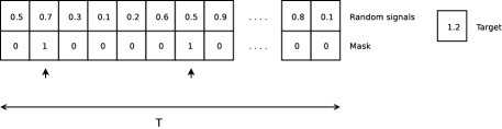
Figure 1: An example of the “adding” problem, where the target is 1.2 which is the sum of 2nd and the 7th numbers in the first sequence [24].

A basic baseline is to always predict the sum to have a value of 1 regardless of the inputs. This will give the Mean Squared Error (MSE) around 0.1767. The goal is to train a model that achieves MSE well below 0.1767.

The problem gets harder as the length of the sequence $T$ increases because the dependency between the output and the relevant inputs becomes more remote. To solve this problem, the recurrent net must remember the first number or the sum of the two numbers accurately whilst ignoring all of the irrelevant numbers.

We generated a training set of 100,000 examples and a test set of 10,000 examples as we varied $T$. We fixed the hidden states to have $100$ units for all of our networks (LSTMs, RNNs and IRNNs). This means the LSTMs had more parameters by a factor of about 4 and also took about 4 times as much computation per timestep.

As we varied $T$, we noticed that both LSTMs and RNNs started to struggle when $T$ is around 150. We therefore focused on investigating the behaviors of all models from this point onwards. The results of the experiments with $T=150,T=200,T=300,T=400$ are reported in figure 2 below (best hyperparameters found during grid search are listed in table 1).

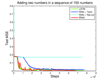
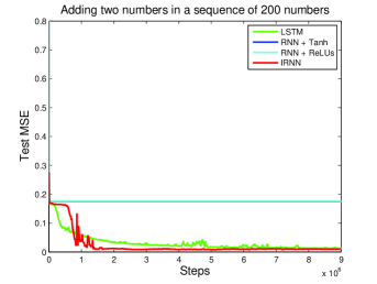
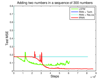
Figure 2: The results of recurrent methods on the “adding” problem for the case of $T=150$ (top left), $T=200$ (top right), $T=300$ (bottom left) and $T=400$ (bottom right). The objective function is the Root Mean Squared Error, reported on the test set of 10,000 examples. Note that always predicting the sum to be 1 should give MSE of 0.1767.

T	LSTM	RNN + Tanh	IRNN
150	$lr=0.01,gc=10,fb=1.0$	$lr=0.01,gc=100$	$lr=0.01,gc=100$
200	$lr=0.001,gc=100,fb=4.0$	N/A	$lr=0.01,gc=1$
300	$lr=0.01,gc=1,fb=4.0$	N/A	$lr=0.01,gc=10$
400	$lr=0.01,gc=100,fb=10.0$	N/A	$lr=0.01,gc=1$

Table 1: Best hyperparameters found for adding problems after grid search. $lr$ is the learning rate, $gc$ is gradient clipping, and $fb$ is forget gate bias. N/A is when there is no hyperparameter combination that gives good result.

The results show that the convergence of IRNNs is as good as LSTMs. This is given that each LSTM step is more expensive than an IRNN step (at least 4x more expensive). Adding two numbers in a sequence of 400 numbers is somewhat challenging for both algorithms.

4.2 MNIST Classification from a Sequence of Pixels

Another challenging toy problem is to learn to classify the MNIST digits [21] when the 784 pixels are presented sequentially to the recurrent net. In our experiments, the networks read one pixel at a time in scanline order (i.e. starting at the top left corner of the image, and ending at the bottom right corner). The networks are asked to predict the category of the MNIST image only after seeing all 784 pixels. This is therefore a huge long range dependency problem because each recurrent network has 784 time steps.

To make the task even harder, we also used a fixed random permutation of the pixels of the MNIST digits and repeated the experiments.

All networks have 100 recurrent hidden units. We stop the optimization after it converges or when it reaches 1,000,000 iterations and report the results in figure 3 (best hyperparameters are listed in table 2).

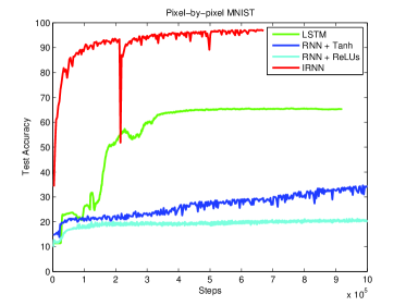
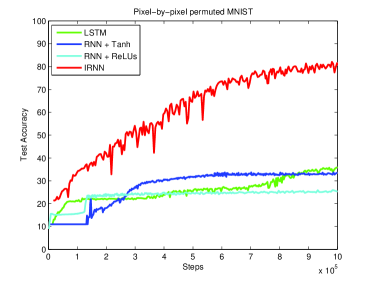
Figure 3: The results of recurrent methods on the “pixel-by-pixel MNIST” problem. We report the test set accuracy for all methods. Left: normal MNIST. Right: permuted MNIST.

Problem	LSTM	RNN + Tanh	RNN + ReLUs	IRNN
MNIST	$lr=0.01,gc=1$	$lr=10^{-8},gc=10$	$lr=10^{-8},gc=10$	$lr=10^{-8},gc=1$
	$fb=1.0$
permuted	$lr=0.01,gc=1$	$lr=10^{-8},gc=1$	$lr=10^{-6},gc=10$	$lr=10^{-9},gc=1$
MNIST	$fb=1.0$

Table 2: Best hyperparameters found for pixel-by-pixel MNIST problems after grid search. $lr$ is the learning rate, $gc$ is gradient clipping, and $fb$ is the forget gate bias.

The results using the standard scanline ordering of the pixels show that this problem is so difficult that standard RNNs fail to work, even with ReLUs, whereas the IRNN achieves 3% test error rate which is better than most off-the-shelf linear classifiers [21]. We were surprised that the LSTM did not work as well as IRNN given the various initialization schemes that we tried. While it still possible that a better tuned LSTM would do better, the fact that the IRNN perform well is encouraging.

Applying a fixed random permutation to the pixels makes the problem even harder but IRNNs on the permuted pixels are still better than LSTMs on the non-permuted pixels.

The low error rates of the IRNN suggest that the model can discover long range correlations in the data while making weak assumptions about the inputs. This could be important to have for problems when input data are in the form of variable-sized vectors (e.g. the repeated field of a protobuffer ).

4.3 Language Modeling

We benchmarked RNNs, IRNNs and LSTMs on the one billion word language modelling dataset [2], perhaps the largest public benchmark in language modeling. We chose an output vocabulary of 1,000,000 words.

As the dataset is large, we observed that the performance of recurrent methods depends on the size of the hidden states: they perform better as the size of the hidden states gets larger (cf. [2]). We however focused on a set of simple controlled experiments to understand how different recurrent methods behave when they have a similar number of parameters. We first ran an experiment where the number of hidden units (or memory cells) in LSTM are chosen to be 512. The LSTM is trained for 60 hours using 32 replicas. Our goal is then to check how well IRNNs perform given the same experimental environment and settings. As LSTM have more parameters per time step, we compared them with an IRNN that had 4 layers and same number of hidden units per layer (which gives approximately the same numbers of parameters).

We also experimented shallow RNNs and IRNNs with 1024 units. Since the output vocabulary is large, we projected the 1024 hidden units to a linear layer with 512 units before the softmax. This avoids greatly increasing the number of parameters.

The results are reported in table 3, which show that the performance of IRNNs is closer to the performance of LSTMs for this large-scale task than it is to the performance of RNNs.

Methods	Test perplexity
LSTM (512 units)	68.8
IRNN (4 layers, 512 units)	69.4
IRNN (1 layer, 1024 units + linear projection with 512 units before softmax)	70.2
RNN (4 layer, 512 tanh units)	71.8
RNN (1 layer, 1024 tanh units + linear projection with 512 units before softmax)	72.5

Table 3: Performances of recurrent methods on the 1 billion word benchmark.

4.4 Speech Recognition

We performed Phoneme recognition experiments on TIMIT with IRNNs and Bidirectional IRNNs and compared them to RNNs, LSTMs and Bidirectional LSTMs and RNNs. Bidirectional LSTMs have been applied previously to TIMIT in [11]. In these experiments we generated phoneme alignments from Kaldi [29] using the recipe reported in [17] and trained all RNNs with two and five hidden layers. Each model was given log Mel filter bank spectra with their delta and accelerations, where each frame was 120 (=40*3) dimensional and trained to predict the phone state (1 of 180). Frame error rates (FER) from this task are reported in table 4.

Methods	Frame error rates (dev / test)
RNN (500 neurons, 2 layers)	35.0 / 36.2
LSTM (250 cells, 2 layers)	34.5 / 35.4
iRNN (500 neurons, 2 layers)	34.3 / 35.5
RNN (500 neurons, 5 layers)	35.6 / 37.0
LSTM (250 cells, 5 layers)	35.0 / 36.2
iRNN (500 neurons, 5 layers)	33.0 / 33.8
Bidirectional RNN (500 neurons, 2 layers)	31.5 / 32.4
Bidirectional LSTM (250 cells, 2 layers)	29.6 / 30.6
Bidirectional iRNN (500 neurons, 2 layers)	31.9 / 33.2
Bidirectional RNN (500 neurons, 5 layers)	33.9 / 34.8
Bidirectional LSTM (250 cells, 5 layers)	28.5 / 29.1
Bidirectional iRNN (500 neurons, 5 layers)	28.9 / 29.7

Table 4: Frame error rates of recurrent methods on the TIMIT phone recognition task.

In this task, instead of the identity initialization for the IRNNs matrices we used $0.01I$ so we refer to them as iRNNs. Initalizing with the full identity led to slow convergence, worse results and sometimes led to the model diverging during training. We hypothesize that this was because in the speech task similar inputs are provided to the neural net in neighboring frames. The normal IRNN keeps integrating this past input, instead of paying attention mainly to the current input because it has a difficult time forgetting the past. So for the speech task, we are not only showing that iRNNs work much better than RNNs composed of tanh units, but we are also showing that initialization with the full identity is suboptimal when long range effects are not needed. Mulitplying the identity with a small scalar seems to be a good remedy in such cases.

In general in the speech recognition task, the iRNN easily outperforms the RNN that uses tanh units and is comparable to LSTM although we don’t rule out the possibility that with very careful tuning of hyperparameters, the relative performance of LSTMs or the iRNNs might change. A five layer Bidirectional LSTM outperforms all the other models on this task, followed closely by a five layer Bidirectional iRNN.

4.5 Acknowledgements

We thank Jeff Dean, Matthieu Devin, Rajat Monga, David Sussillo, Ilya Sutskever and Oriol Vinyals for their help with the project.

References

- [1] D. Bahdanau, K. Cho, and Y. Bengio. Neural machine translation by jointly learning to align and translate. arXiv preprint arXiv:1409.0473, 2014.
- [2] C. Chelba, T. Mikolov, M. Schuster, Q. Ge, T. Brants, and P. Koehn. One billion word benchmark for measuring progress in statistical language modeling. CoRR, abs/1312.3005, 2013.
- [3] G. E. Dahl, D. Yu, L. Deng, and A. Acero. Context-dependent pre-trained deep neural networks for large vocabulary speech recognition. IEEE Transactions on Audio, Speech, and Language Processing - Special Issue on Deep Learning for Speech and Language Processing, 2012.
- [4] J. Dean, G. S. Corrado, R. Monga, K. Chen, M. Devin, Q. V. Le, M. Z. Mao, M. A. Ranzato, A. Senior, P. Tucker, K. Yang, and A. Y. Ng. Large scale distributed deep networks. In NIPS, 2012.
- [5] J. Duchi, E. Hazan, and Y. Singer. Adaptive subgradient methods for online learning and stochastic optimization. The Journal of Machine Learning Research, 12:2121–2159, 2011.
- [6] F. A. Gers, J. Schmidhuber, and F. Cummins. Learning to forget: Continual prediction with LSTM. Neural Computation, 2000.
- [7] F. A. Gers, N. N. Schraudolph, and J. Schmidhuber. Learning precise timing with lstm recurrent networks. The Journal of Machine Learning Research, 2003.
- [8] A. Graves. Generating sequences with recurrent neural networks. arXiv preprint arXiv:1308.0850, 2013.
- [9] A. Graves. Generating sequences with recurrent neural networks. In Arxiv, 2013.
- [10] A. Graves and N. Jaitly. Towards end-to-end speech recognition with recurrent neural networks. In Proceedings of the 31st International Conference on Machine Learning, 2014.
- [11] A. Graves, N. Jaitly, and A-R. Mohamed. Hybrid speech recognition with deep bidirectional lstm. In IEEE Workshop on Automatic Speech Recognition and Understanding (ASRU),, 2013.
- [12] A. Graves, M. Liwicki, S. Fernández, R. Bertolami, H. Bunke, and J. Schmidhuber. A novel connectionist system for unconstrained handwriting recognition. IEEE Transactions on Pattern Analysis and Machine Intelligence, 2009.
- [13] A. Graves, A-R. Mohamed, and G. Hinton. Speech recognition with deep recurrent neural networks. In IEEE International Conference on Acoustics, Speech and Signal Processing (ICASSP), 2013.
- [14] G. Hinton. Lecture 6.5-rmsprop: Divide the gradient by a running average of its recent magnitude. COURSERA: Neural Networks for Machine Learning, 2012.
- [15] S. Hochreiter, Y. Bengio, P. Frasconi, and J. Schmidhuber. Gradient flow in recurrent nets: the difficulty of learning long-term dependencies. A Field Guide to Dynamical Recurrent Neural Networks, 2001.
- [16] S. Hochreiter and J. Schmidhuber. Long short-term memory. Neural Computation, 1997.
- [17] N. Jaitly. Exploring Deep Learning Methods for discovering features in speech signals. PhD thesis, University of Toronto, 2014.
- [18] R. Kiros, R. Salakhutdinov, and R. S. Zemel. Unifying visual-semantic embeddings with multimodal neural language models. arXiv preprint arXiv:1411.2539, 2014.
- [19] A. Krizhevsky, I. Sutskever, and G. E. Hinton. Imagenet classification with deep convolutional neural networks. In Advances in Neural Information Processing Systems, 2012.
- [20] Q. V. Le, M. A. Ranzato, R. Monga, M. Devin, K. Chen, G. S. Corrado, J. Dean, and A. Y. Ng. Building high-level features using large scale unsupervised learning. In International Conference on Machine Learning, 2012.
- [21] Y. LeCun, L. Bottou, Y. Bengio, and P. Haffner. Gradient-based learning applied to document recognition. Proceedings of the IEEE, 1998.
- [22] T. Luong, I. Sutskever, Q. V. Le, O. Vinyals, and W. Zaremba. Addressing the rare word problem in neural machine translation. arXiv preprint arXiv:1410.8206, 2014.
- [23] J. Martens. Deep learning via Hessian-free optimization. In Proceedings of the 27th International Conference on Machine Learning, 2010.
- [24] J. Martens and I. Sutskever. Learning recurrent neural networks with Hessian-Free optimization. In ICML, 2011.
- [25] J. Martens and I. Sutskever. Training deep and recurrent neural networks with Hessian-Free optimization. Neural Networks: Tricks of the Trade, 2012.
- [26] T. Mikolov, A. Joulin, S. Chopra, M. Mathieu, and M. A. Ranzato. Learning longer memory in recurrent neural networks. arXiv preprint arXiv:1412.7753, 2014.
- [27] V. Nair and G. Hinton. Rectified Linear Units improve Restricted Boltzmann Machines. In International Conference on Machine Learning, 2010.
- [28] R. Pascanu, T. Mikolov, and Y. Bengio. On the difficulty of training recurrent neural networks. arXiv preprint arXiv:1211.5063, 2012.
- [29] D. Povey, A. Ghoshal, G. Boulianne, L. Burget, O. Glembek, N. Goel, M. Hannemann, P. Motlicek, Y. Qian, P. Schwarz, J. Silovsky, G. Stemmer, and K. Vesely. The kaldi speech recognition toolkit. In IEEE 2011 Workshop on Automatic Speech Recognition and Understanding. IEEE Signal Processing Society, 2011.
- [30] D. Rumelhart, G. E. Hinton, and R. J. Williams. Learning representations by back-propagating errors. Nature, 323(6088):533–536, 1986.
- [31] A. M. Saxe, J. L. McClelland, and S. Ganguli. Exact solutions to the nonlinear dynamics of learning in deep linear neural networks. arXiv preprint arXiv:1312.6120, 2013.
- [32] R. Socher, J. Bauer, C. D. Manning, and A. Y. Ng. Parsing with compositional vector grammars. In ACL, 2013.
- [33] D. Sussillo and L. F. Abbott. Random walk intialization for training very deep networks. arXiv preprint arXiv:1412.6558, 2015.
- [34] I. Sutskever, J. Martens, G. Dahl, and G. Hinton. On the importance of initialization and momentum in deep learning. In Proceedings of the 30th International Conference on Machine Learning, 2013.
- [35] I. Sutskever, J. Martens, and G. E. Hinton. Generating text with recurrent neural networks. In Proceedings of the 28th International Conference on Machine Learning, pages 1017–1024, 2011.
- [36] I. Sutskever, O. Vinyals, and Q. V. Le. Sequence to sequence learning with neural networks. In NIPS, 2014.
- [37] O. Vinyals, L. Kaiser, T. Koo, S. Petrov, I. Sutskever, and G. Hinton. Grammar as a foreign language. arXiv preprint arXiv:1412.7449, 2014.
- [38] O. Vinyals, A. Toshev, S. Bengio, and D. Erhan. Show and tell: A neural image caption generator. arXiv preprint arXiv:1411.4555, 2014.
- [39] W. Zaremba and I. Sutskever. Learning to execute. arXiv preprint arXiv:1410.4615, 2014.
- [40] M. Zeiler, M. Ranzato, R. Monga, M. Mao, K. Yang, Q. V. Le, P. Nguyen, A. Senior, V. Vanhoucke, and J. Dean. On rectified linear units for speech processing. In IEEE Conference on Acoustics, Speech and Signal Processing (ICASSP), 2013.