Straintronic spin-neuron

Abstract

In artificial neural networks, neurons are usually implemented with highly dissipative CMOS-based operational amplifiers. A more energy-efficient implementation is a “spin-neuron” realized with a magneto-tunneling junction (MTJ) that is switched with a spin-polarized current (representing weighted sum of input currents) that either delivers a spin transfer torque or induces domain wall motion in the soft layer of the MTJ. Here, we propose and analyze a different type of spin-neuron in which the soft layer of the MTJ is switched with mechanical strain generated by a voltage (representing weighted sum of input voltages) and term it straintronic spin-neuron. It dissipates orders of magnitude less energy in threshold operations than the traditional current-driven spin neuron at 0 K temperature and may even be faster. We have also studied the room-temperature firing behaviors of both types of spin neurons and find that thermal noise degrades the performance of both types, but the current-driven type is degraded much more than the straintronic type if both are optimized for maximum energy-efficiency. On the other hand, if both are designed to have the same level of thermal degradation, then the current-driven version will dissipate orders of magnitude more energy than the straintronic version. Thus, the straintronic spin-neuron is superior to current-driven spin neurons.

Keywords: spin-neuron, neural network, straintronics, nanomagnets

1 Introduction

The building blocks of neural computing architectures are ‘neurons’ usually connected to each other and to external stimuli through programmable ‘synapses’. The transfer function of a neuron can be expressed as

$$O=f\left(\sum_{i}w_{i}x_{i}+b\right)$$ (1)

where $f$ is some nonlinear function, $w_{i}$-s are programmable weights of synapses, $x_{i}$-s are the input signals (representing dendrites), $b$ is a fixed bias and $O$ is the output (representing a neuron’s axon). In threshold operations, $f$ mimics a Heaviside unit step function whose value is 1 if the argument is positive and 0 otherwise.

Neural networks have myriad topologies, such as cellular neural network [1], feed-forward network [2], convolutional neural network [3], hierarchical temporal memory [4], etc. However, the basic unit of computing i.e., the neuron, remains more or less invariant across all topologies and its operation is governed by Equation (1). In a conventional neural network, CMOS operational amplifiers carry out the threshold operation of Equation (1) [5] and dissipate exorbitant amounts of energy. To a large extent, this has stymied the progress of neural computing. Alternate implementations to lower the energy dissipation have been proposed in recent years [6, 7, 8] and utilize a magneto-tunneling junction (MTJ) whose soft layer is an anisotropic nanomagnet with two stable magnetization orientations. Input variables are encoded in spin-polarized currents that are summed with variable weights to produce a net spin polarized current which is driven through the nanomagnet. When the net current exceeds a threshold value, the magnetization of the soft layer rotates from one stable orientation to the other, thereby changing the resistance of the MTJ abruptly. This implements the threshold firing behavior of a neuron. These types of artificial neurons have been termed ‘spin-neurons’ and unlike CMOS-based neurons, they are ‘non-volatile’ since the final state of the neuron can be stored in the magnetization state of the nanomagnet (and therefore the resistance of the MTJ) after the device is powered down. In Ref. [8], the soft layer of the MTJ is a nanomagnet possessing perpendicular magnetic anisotropy (see Figure 3(a) of Ref. [8]) and it is switched with spin-polarized current generated via the giant spin Hall effect [9] which induces domain wall motion. This type of spin neurons belongs to the general class of (spin-polarized) current driven artificial neurons.

In this paper we propose and analyze a different type of spin-neuron implemented with MTJs having soft layers that are magnetostrictive or multiferroic nanomagnets and whose magnetizations are flipped with mechanical stress/strain generated by a voltage. We call them ‘straintronic spin-neurons’ and they are voltage-driven as opposed to current-driven. This has the advantage of further reducing the energy dissipation during firing. Switching of multiferroic nanomagnets with voltage-generated stress has been proposed and/or demonstrated by many groups [10, 11, 12, 13, 14] and is particularly useful for writing bits in non-volatile memory [15, 16, 17, 18, 19, 20]. It can be also harnessed for logic applications [12, 21, 22, 23] and results in exceptionally low dissipation. Here, we propose it for neural applications. We compare the energy-efficiency of a straintronic spin neuron with that of a traditional current-driven spin neuron and show that the former is more energy efficient. Finally, since magnetization dynamics is vulnerable to thermal noise, we study the operation of spin-neurons at room temperature in the presence of thermal noise and compare that with 0 K operation to assess the degree of thermal degradation. As expected, thermal noise has a deleterious effect on the threshold behavior and seriously degrades the abruptness of the firing action. The degradation is far worse for the current-driven type than for the straintronic type.

2 Straintronic Spin Neuron

Figure 1 shows the schematic of a straintronic spin-neuron with programmable synapses. Inputs $x_{i}$-s and the bias $b$ are in the form of voltages $V_{i}$-s and $b$, the latter being realized with a constant current source $I$ [$b=I\left(R_{1}\parallel R_{2}\parallel r_{1}\parallel r_{2}\parallel\cdot\cdot\cdot\parallel r_{N-1}\parallel r_{N}\right)$]. The voltage appearing at node $P$ is dropped across the piezoelectric layer underneath the (shorted) contact pads A and A^′. It is a weighted sum of input voltages and bias, and is given by

$$V_{P}=\sum_{i=1}^{N}w_{i}V_{i}+b,$$ (2)

where $w_{i}={{R_{1}\parallel R_{2}\parallel r_{1}\parallel r_{2}\parallel\cdot\cdot\cdot\parallel r_{i-1}\parallel r_{i+1}\parallel\cdot\cdot\cdot\parallel r_{N}}\over{R_{1}\parallel R_{2}\parallel r_{1}\parallel r_{2}\parallel\cdot\cdot\cdot\parallel r_{i-1}\parallel r_{i+1}\parallel\cdot\cdot\cdot\parallel r_{N}+r_{i}}}$. The resistances $R_{1},R_{2}$ are the resistances of the piezoelectric layer underneath the contact pads and $r_{i}$-s are the series resistances (connected to the input terminals) that implement the programmable weights. Equation (2) is obtained from voltage superposition.

The magneto-tunneling junction (MTJ) in Figure 1 is the central unit of the neuron. It has a hard nanomagnet, a spacer layer and a soft magnetostrictive nanomagnet in contact with the piezoelectric. All nanomagnets are shaped like elliptical disks. A bias magnetic field $B$ in the plane of the soft nanomagnet directed along its minor axis makes the magnetization orientation of the soft nanomagnet bistable, with the two stable directions shown as $\Psi_{\parallel}$ and $\Psi_{\perp}$ which subtend an angle of $\sim$90^∘ between them [15]. The hard nanomagnet is implemented with a synthetic anti-ferromagnet and its two stable magnetization orientations are roughly along its major axis because of the extremely high shape anisotropy that this nanomagnet possesses. The hard nanomagnet is placed such that its major axis is collinear with one of the stable magnetization orientations of the soft nanomagnet (say $\Psi_{\parallel}$), resulting in a “skewed MTJ stack” where the major axes of the two nanomagnets are at an angle. The hard nanomagnet is then magnetized permanently in the direction that is anti-parallel to $\Psi_{\parallel}$. Thus, when the soft nanomagnet is in the stable state $\Psi_{\parallel}$, the magnetizations of the hard and soft layers of the MTJ are mutually anti-parallel, resulting in high MTJ resistance, while when the soft nanomagnet is in the other stable state $\Psi_{\perp}$, the magnetizations of the two layers are roughly perpendicular to each other, resulting in lower MTJ resistance. The ratio of the high-to-low MTJ resistances is approximately $1/\left(1-\eta_{1}\eta_{2}\right)$, where the $\eta$-s are the spin injection/detection efficiencies at the interfaces of the spacer with the two nanomagnets. We assume that at room temperature, $\eta_{1}=\eta_{2}\approx 70\%$ [24] and therefore the resistance ratio will be roughly 2:1. Higher resistance ratios exceeding 6:1 have been demonstrated at room temperature [25], but we will be conservative and assume the ratio to be 2:1.

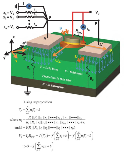
Figure 1: Schematic of a straintronic spin-neuron implementing a step transfer function. The artificial synapses are realized with the passive resistors $r_{1}\cdots r_{n}$.

The electrodes A and A^′ are placed on the piezoelectric layer such that the line joining their centers is parallel to $\Psi_{\parallel}$ and hence also to the major axis of the hard nanomagnet. Their lateral dimensions are of the same order as and the inter-electrode separation is 1-2 times the PZT thin film thickness. When voltages are applied between the electrode pair and the (grounded) conducting substrate, electric fields are generated underneath the electrode pads in the PZT layer as shown in Figure 1. They produce out-of-plane compressive strain and in-plane tensile strain or vice versa, depending on the polarity of the voltage in the PZT layer below the electrodes [26]. These strain fields interact and produce biaxial strain between the electrodes (tensile along the line joining the electrodes and compressive in the perpendicular direction, or vice versa) [26], which is almost completely transferred to the magnetostrictive soft magnet since the latter’s thickness is much smaller than that of the strained PZT layer.

If the magnetostriction coefficient of the soft magnet material is positive (e.g. Terfenol-D), then sufficient compressive stress resulting along the line joining the electrode centers, i.e. in the direction of $\Psi_{\parallel}$, will rotate the soft layer’s magnetization to $\Psi_{\perp}$, while sufficient tensile stress will keep the magnetization aligned along $\Psi_{\parallel}$. The situation will be opposite if the magnetostriction coefficient of the soft magnet is negative (e.g. cobalt). Since, for either sign of the magnetostriction coefficient, the sign of the stress (compressive or tensile) depends on the polarity of the voltage applied between the electrodes and the grounded substrate, the magnetization of the soft magnet can be aligned along either of the two stable orientations $\Psi_{\parallel}$ and $\Psi_{\perp}$ at will by simply choosing the voltage polarities (of the inputs and bias voltages).

There is a minimum stress (compressive/tensile) required to switch the magnetization of the soft nanomagnet of the MTJ from one orientation (say, $\Psi_{\parallel}$) to the other (say, $\Psi_{\perp}$) because the two stable states are separated by an energy barrier [15, 18, 19, 23] that needs to be overcome by stress to make the switching occur. At 0 K temperature, this feature gives rise to a sharp threshold in the switching behavior and makes it possible to mimic the sudden firing behavior of a neuron. The energy barrier (and hence the threshold stress) depends on the permanent magnetic field $B$ and the size and shape of the soft nanomagnet, if we ignore dipole coupling with the hard nanomagnet and any magneto-crystalline anisotropy (the magnets are assumed to be amorphous). These parameters determine the effective in-plane energy barrier between the two stable magnetization states $\Psi_{\parallel}$ and $\Psi_{\perp}$ that must be overcome by stress to switch the magnetization of the soft nanomagnet from one state to the other and therefore the MTJ resistance. The minimum stress needed for switching (also called the ‘critical stress’) at 0 K can be found by equating the stress anisotropy energy to the effective in-plane energy barrier.

The critical stress gives rise to a critical voltage $V_{c}$ for switching at 0 K. When the total voltage $V_{P}$, appearing at node $P$, due to all weighted inputs and the bias, exceeds the critical voltage, the MTJ resistance switches abruptly because the soft layer’s magnetization rotates from one stable orientation to the other. If we bias the MTJ with a constant current source $I_{B}$ as shown in Fig. 1, then the voltage across the MTJ is $V_{MTJ}=I_{B}R_{MTJ}$ where $R_{MTJ}$ is the MTJ resistance that has a non-linear dependence on $V_{P}$ (abrupt switching when $V_{P}$ exceeds $V_{c}$). Because there is virtually no electric field in the PZT layer directly underneath the magnet, we can ignore any potential drop in this region and write the output voltage in Fig. 1 as $V_{0}\approx V_{MTJ}=I_{B}R_{MTJ}$ which has a non-linear dependence on $V_{P}$ and hence exhibits a threshold behavior. Using Equation (2), we can now write

$$V_{0}=f\left(V_{P}\right)=f\left(\sum_{i=1}^{N}w_{i}V_{i}+b\right),$$ (3)

which replicates the neural behavior.

3 Simulation of neuron firing with the Landau-Lifshitz-Gilbert (LLG) equation

We will design our straintronic spin-neuron by choosing the dimensions of the nanomagnet and the magnitude of the permanent magnetic field to select the critical voltage $V_{c}$, and therefore the firing threshold. We choose a soft nanomagnet of major axis $a$ = 100 nm, minor axis $b$ = 42 nm and thickness $d$ = 16.5 nm, which ensures that it has a single ferromagnetic domain [27]. When stress is applied on the soft nanomagnet by applying the voltage $V_{P}$ at the electrodes A and A^′, which is the weighted sum of the inputs and bias, the magnetization vector of the soft nanomagnet experiences a torque that makes it rotate and ultimately switch the MTJ resistance. The torque depends on the shape anisotropy energy of the soft nanomagnet, the permanent magnetic field and the stress.

The shape anisotropy energy is a function of the time-dependent magnetization orientation during switching and can be written as

$$E_{sh}(t) = E_{s1}(t){\sin}^{2}{\theta^{\prime}(t)}+E_{s2}(t){\sin 2\theta^{\prime}(t)}+\frac{\mu_{0}}{4}\Omega{M}^{2}_{s}(N_{d-yy}+N_{d-zz})$$

$$E_{s1}(t) = \left(\frac{\mu_{0}}{4}\right)\Omega{M}^{2}_{s}\left(2N_{d-xx}-N_{d-yy}-N_{d-zz}\right){\cos}^{2}{\phi^{\prime}(t)}$$

$$E_{s2}(t) = \left(\frac{\mu_{0}}{4}\right)\Omega{M}^{2}_{s}\left(N_{d-zz}-N_{d-yy}\right){\sin\phi^{\prime}(t)},$$ (4)

where $\theta^{\prime}(t)$ and $\phi^{\prime}(t)$ are, respectively, the instantaneous polar and azimuthal angles of the soft nanomagnet’s magnetization vector in the primed reference frame shown in Figure 1. The unprimed reference frame is such that the z-axis coincides with the soft nanomagnet’s easy axis and y-axis with the hard axis. The primed reference frame is obtained by rotating anticlockwise about the x-axis by 45^∘. The quantity $M_{s}$ is the saturation magnetization of the soft nanomagnet, $N_{d-xx}$, $N_{d-yy}$ and $N_{d-zz}$ are the demagnetization factors that can be evaluated from the nanomagnet’s dimensions [28], $\mu_{0}$ is the permeability of free space, and $\Omega=(\pi/4)abd$ is the soft nanomagnet’s volume.

The permanent magnetic field contributes an additional term to the potential energy of the soft nanomagnet given by

$$E_{m}(t)=\frac{1}{\sqrt{2}}M_{s}\Omega B\left[{\cos\theta^{\prime}(t)}-{\sin\theta^{\prime}(t)}{\sin\phi^{\prime}(t)}\right].$$ (5)

The locations of the total potential energy $\left(E_{sh}(\theta(t),\phi(t))+E_{m}(\theta(t),\phi(t))\right)$ minima (in the absence of stress) determine the stable magnetization orientations of the soft nanomagnet and are found by minimizing the total potential energy with respect to $\theta(t),\phi(t)$. In our case, the two stable orientations (the two degenerate energy minima) turn out to be $\Psi_{\parallel}$ ($\theta=\theta_{1}=46.9^{\circ},\phi=\phi_{1}=90^{\circ}$) and $\Psi_{\perp}$ ($\theta=\theta_{0}=133^{\circ},\phi=\phi_{0}=90^{\circ}=\phi_{1}$) with an angular separation $\gamma$ of 86.1^∘ (Figure 1) between them when B is 0.14 T. The in-plane energy barrier separating these two energy minima is 73.1 kT at room temperature resulting in a tiny probability ($e^{-73.1}\sim 10^{-32}$) of the neuron firing spontaneously at room temperature by switching between the stable states $\Psi_{\parallel}$ and $\Psi_{\perp}$ per attempt. With an attempt frequency of 10¹⁵ Hz, the mean time between successive spontaneous firing (switching of the MTJ) would then be $10^{-15}\times 10^{32}$ = 10¹⁷ seconds = 3$\times$10⁷ centuries.

When voltages are applied at the electrodes A and A^′, the resulting stress produced in the soft nanomagnet contributes a stress anisotropy energy to the soft nanomagnet’s potential energy. Although the generated strain is biaxial, we will approximate it as uniaxial strain to somewhat compensate for the fact that not 100% of the strain in the PZT will be transferred to the soft nanomagnet. With this assumption, the stress anisotropy energy is written as

$$E_{str}(t)=-\frac{3}{2}\lambda_{s}\epsilon(t)Y\Omega{\cos}^{2}{\theta^{\prime}(t)},$$ (6)

where $\lambda_{s}$ is the magnetostriction coefficient of the soft nanomagnet, $Y$ is the Young’s modulus, and $\epsilon(t)$ is the strain generated by the applied voltage $V_{P}(t)$ at the instant of time $t$.

The total potential energy of a stressed nanomagnet at any instant of time $t$ is therefore

$$E(t)=E\left(\theta^{\prime}(t),\phi^{\prime}(t)\right)=E_{sh}(t)+E_{m}(t)+E_{str}(t).$$ (7)

We follow the standard procedure to derive the time evolution of the polar and azimuthal angles of the magnetization vector of the soft nanomagnet in the rotated coordinate frame under the actions of the torques due to shape anisotropy, stress anisotropy and magnetic field by solving the Landau-Lifshitz-Gilbert (LLG) equation:

$$\frac{d\mathbf{m}(t)}{dt} - \alpha\left[\mathbf{m}(t)\times\frac{d\mathbf{m}(t)}{dt}\right]=\frac{-|\gamma|}{\mu_{0}M_{s}\Omega}\mathbf{\tau_{ss}}(t),$$ (8)

where $\alpha$ is the Gilbert damping coefficient which depends on the soft nanomagnet’s material, $\gamma$ is the gyromagnetic ratio (a universal constant) and $\tau_{ss}$ is the total torque acting on the magnetization vector and is given by

$$\mathbf{\tau_{ss}}(t) = -\mathbf{m}(t)\times\left(\frac{\partial E(t)}{\partial\theta^{\prime}(t)}\hat{\boldsymbol{\theta}}+\frac{1}{\sin\theta^{\prime}(t)}\frac{\partial E(t)}{\partial\phi^{\prime}(t)}\hat{\boldsymbol{\phi}}\right)$$ (9)

$$= \{E_{\phi 1}(t)\sin\theta^{\prime}(t)+E_{\phi 2}(t)\cos\theta^{\prime}(t)$$

$$- \frac{1}{\sqrt{2}}M_{s}\Omega B\cos\phi^{\prime}(t)\}\hat{\boldsymbol{\theta}}$$

$$- \{E_{s1}(t)\sin 2\theta^{\prime}(t)+2E_{s2}(t)\cos 2\theta^{\prime}(t)$$

$$- \frac{1}{\sqrt{2}}M_{s}\Omega B(\sin\phi^{\prime}(t)\cos\theta^{\prime}(t)+\sin\theta^{\prime}(t))$$

$$+ (3/2)\lambda_{s}\epsilon(t)Y\Omega\sin 2\theta^{\prime}(t)\}\hat{\boldsymbol{\phi}},$$

where $\mathbf{m}(t)$ is the normalized magnetization vector, quantities with carets are unit vectors in the original frame of reference, and

$$E_{\phi 1}(t) = \frac{\mu_{0}}{4}{M}^{2}_{s}\Omega\{\left(N_{d-yy}+N_{d-zz}\right)\sin 2\phi^{\prime}(t)-2N_{d-xx}\sin 2\phi^{\prime}(t)\}$$

$$E_{\phi 2}(t) = \frac{\mu_{0}}{2}{M}^{2}_{s}\Omega\left(N_{d-zz}-N_{d-yy}\right)\cos\phi^{\prime}(t).$$

At non-zero temperatures, there is an additional torque acting on the magnetization vector owing to thermal noise. The procedure for finding this torque has been described in Ref. [29] and is not repeated here.

Solution of the LLG equation [Equation (8)] yields the magnetization of the stressed soft nanomagnet as a function of time and steady state is achieved when the magnetization no longer changes appreciably with time. This yields the switching time (time elapsed before reaching steady-state) and the energy dissipation for any given stress. The procedure for finding these quantities in the presence of thermal fluctuations requires solving the stochastic LLG equation and is described in Ref. [29] and [30].

We assume that the soft nanomagnet is made of Terfenol-D which has the following material parameters: saturation magnetization $M_{s}=$ 8 $\times$ 10⁵ A/m, magnetostriction coefficient $\lambda_{s}=$ 60 $\times$ 10^-5 , Young’s modulus $Y$ = 80 GPa and Gilbert damping coefficient $\alpha=$ 0.1 [31, 32, 33].

We solve the Landau-Lifshitz-Gilbert equation [Equation (8)] at 0 K (and its stochastic version at 300 K) to find the steady-state orientation of the magnetization vector of the soft nanomagnet as a function of stress in the nanomagnet and therefore as a function of the sum-total voltage applied at the electrode pairs. The stress is varied between -50 and +50 MPa. By following the procedure in Ref. [26], we compute that an electric field of 37.5 kV/m is required to produced a stress of 1 MPa in the PZT, which we assume is fully transferred to the soft magnet. Therefore, assuming that stress is linearly proportional to the voltage, the corresponding voltages for $\pm$50 MPa are $\pm$187.5 mV if the PZT film’s thickness is 100 nm.

At the critical stress value (or critical voltage), the soft layer’s magnetization vector changes abruptly from its initial stable orientation to the other causing the angle between the magnetizations of the soft and hard layer to change from $\beta_{L}=180^{\circ}-86.1^{\circ}=93.9^{\circ}$ to $\beta_{H}=180^{\circ}$, or vice versa. This will cause the S-MTJ resistance to change by a factor of $\left(1+\eta_{1}\eta_{2}cos(93.9^{\circ})\right)/\left(1-\eta_{1}\eta_{2}\right)$ $\sim$ 1.9 if we assume $\eta_{1}=\eta_{2}=0.7$.

Figure 2 shows the ratio $R(V)/R_{L}$ as a function of voltage $V$ applied at the contact pads, where $R(V)$ is the MTJ resistance at a voltage $V$ and $R_{L}$ is the MTJ resistance in the low-resistance state. If the MTJ is initially in the high resistance state, a compressive stress (positive voltage) is required to drive it to the low resistance state, whereas if it is initially in the low resistance state, a tensile stress (negative voltage) is required to drive it to the high resistance state because we have assumed the soft magnet material to be Terfenol-D which has positive magnetostriction. Thus, the critical voltage to switch from high-to-low resistance is +93.15 mV and the critical voltage to switch from low-to-high resistance is -93.15 mV, which produces the appearance of a ‘hysteresis’ in the characteristic in Fig. 2. This hysteretic behavior indicates that the device can also be used as a non-volatile memory. Note that the transitions are not completely abrupt even at 0 K temperature because sub-critical stress that is slightly lower than the critical stress can cause some rotation of the soft magnet’s magnetization vector and hence change the MTJ resistance perceptibly. This is the reason for the ‘rounded corners’.

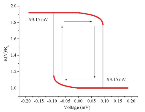
Figure 2: The transfer function (or firing behavior) for a straintronic spin neuron at 0 K. When the voltage appearing at node $P$ (in Figure 1) due to weighted inputs and bias is $V$, the resistance of the MTJ is $R(V)$. The low resistance is $R_{L}$.

The energy dissipated during a firing event is the sum of the $CV^{2}$ dissipation associated with charging the capacitance of the electrodes A and A^′, and the internal dissipation in the soft magnet due to Gilbert damping. We neglect any dissipation due to the current sources assuming that the currents are small and the current sources are turned on only when the inputs arrive. Here, $C$ is the capacitance of the electrodes and $V$ is the voltage at the electrodes. The capacitance is determined from the areas of the electrodes, the dielectric constant of PZT and the PZT film thickness. It is found to be 0.88fF. Therefore, the capacitance charging dissipation will be $2\times(1/2)CV^{2}$ = 0.09315² $\times$ 0.88fF = 7.63 aJ (there are two electrodes A and A^′). The dissipation due to Gilbert damping at 0 K was found to be 1.2 aJ from the solution of the LLG equation as described in Ref. [29] and [34]. Therefore, the total dissipation during a firing event is 8.83 aJ. This is $\sim$450 times lower than that reported (4 fJ) in Ref. [8] for current-driven spin neurons when the input voltage level was 100 mV and $\sim$45 times lower than that (0.4 fJ) when the input voltage level was 10 mV (our input voltage level is $\sim$ 93 mV). Note that the synapse resistances $r_{1}\cdot\cdot\cdot r_{N}$ can be set arbitrarily high and hence the dissipation in them can be neglected. The switching (firing) delay is found to be 1.37 ns at the threshold voltage level.

4 Current-driven Spin Neuron Based on Spin Transfer Torque (STT) switched MTJ

In this section, we discuss a spin-neuron implemented with the same type of MTJ as above, except this time the soft magnet is not switched with strain, but with a spin polarized current delivering a spin transfer torque (STT). The inputs are therefore not voltages, but currents. We choose the material to be CoFeB with in-plane anisotropy which has a Gilbert damping constant of $\sim$0.004 [35], much lower than that of Terfenol-D. This material has in-plane anisotropy if the magnet thickness exceeds a few nm [36]. STT-driven spin neurons built with magnets exhibiting perpendicular anisotropy have been studied in Refs. [8] and [37].

Note that we chose two different materials – Terfenol-D for the straintronic neuron and CoFeB for the current driven neuron – because we wish to optimize both for minimal energy dissipation and then make a fair comparison. Terfenol-D has a very large magnetostriction coefficient and is hence beneficial for a straintronic neuron. A current driven neuron does not benefit from large magnetostriction, but benefits from small Gilbert damping, which is why we chose CoFeB for it.

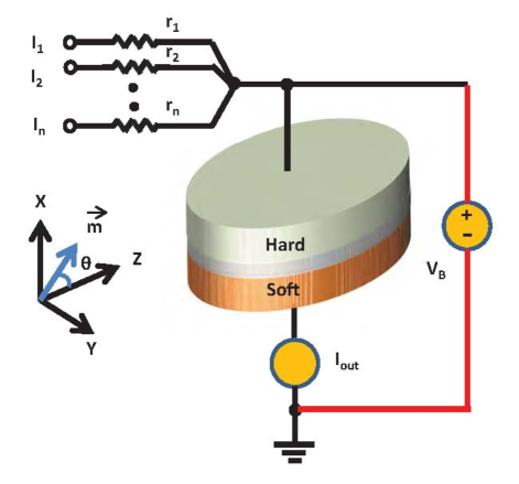
Figure 3: Schematic of a current-driven spin-neuron

Figure 3 shows the schematic of a STT-based current-driven spin neuron consisting of an MTJ stack that is not skewed. Both magnets are elliptical in shape and each has two stable magnetization orientations along the major axis of the ellipse. Their major axes are collinear.

The hard magnet is permanently magnetized along one of its stable orientations. The soft magnet’s magnetization can be either parallel (low-resistance state) or anti-parallel (high-resistance state) to that of the hard magnet. The high-to-low resistance ratio in this case is $\left(1+\eta_{1}\eta_{2}\right)/\left(1-\eta_{1}\eta_{2}\right)$ = 2.9, assuming once again that $\eta_{1}=\eta_{2}=0.7$ [24]. This corresponds to a tunneling magnetoresistance ratio, or TMR, of $\sim$200%.

A negative potential applied between the hard and soft layers will align the magnetization of the soft layer parallel to that of the hard layer (low MTJ resistance), while a positive potential will make it anti-parallel (high MTJ resistance). These potentials cause a spin polarized current to be injected into or extracted from the soft layer which brings about the magnetization switching by exerting a spin-transfer-torque on the magnetization vector [38, 39, 40, 41]. For consistency, the soft layer’s dimensions are chosen such that the in-plane shape anisotropy energy barrier is 71.7 kT, close to that of the soft magnet in the straintronic spin neuron. This is ensured by choosing the major axis $a$ = 50 nm, minor axis $b$ = 32 nm and thickness $d$ = 5 nm [28].

In the absence of spin polarized current, the soft nanomagnet has only shape anisotropy energy and its potential energy at any instant of time $t$ is given by,

$$E_{shape}(t)=E_{ss}(t){\sin}^{2}{\theta(t)}+\frac{\mu_{0}}{2}\Omega{M}^{2}_{s}N_{d-zz}$$

$$E_{ss}(t) =\left(\frac{\mu_{0}}{2}\right)\Omega{M}^{2}_{s}\{N_{d-xx}{\cos}^{2}{\phi(t)}+N_{d-yy}{\sin}^{2}{\phi(t)}-N_{d-zz}\},$$ (10)

where $\theta(t)$ and $\phi(t)$ are again, respectively, the instantaneous polar and azimuthal angles of the magnetization vector, and $M_{s}$ is the saturation magnetization which is $\sim$10.4 $\times$ 10⁵ A/m [42] for amorphous CoFeB.

The torque on the magnetization vector at any time $t$ due to shape anisotropy can be expressed as

$$\mathbf{\tau_{ss}}(t) = -\mathbf{m}(t)\times\left(\frac{\partial E(t)}{\partial\theta(t)}\hat{\boldsymbol{\theta}}+\frac{1}{\sin\theta(t)}\frac{\partial E(t)}{\partial\phi(t)}\hat{\boldsymbol{\phi}}\right)$$ (11)

$$= E_{\phi s}(t)\sin\theta(t)\hat{\boldsymbol{\theta}}-E_{ss}(t)\sin 2\theta(t)\hat{\boldsymbol{\phi}},$$

where $\mathbf{m}(t)$ is the normalized magnetization vector and
$E_{\phi s}(t)\!=\!\{\frac{\mu_{0}}{2}{M}^{2}_{s}\left(N_{d-yy}-N_{d-xx}\right)\}\Omega\sin 2\phi(t).$

Passage of the spin-polarized current $I_{s}$ through the nanomagnet generates a spin transfer torque (STT) on the magnetization vector given by [43]

$$\mathbf{\tau_{sst}}(t) = s[{\tt b}\sin(\zeta-\theta(t))\hat{\boldsymbol{\phi}}-{\tt c}\sin(\zeta-\theta(t))\hat{\boldsymbol{\theta}}],$$ (12)

where $s=(\hbar/2e)\chi I_{s}$ is the spin angular deposition per unit time, $\chi$ is the spin polarization of the current, b and c are coefficients of the out-of-plane and in-plane components of the spin-transfer-torque. We assume $\chi$ = 70% (assuming 70% spin injection efficiency), and b and c are 0.3 and 1, respectively. The current is passed perpendicular to the plane of the magnet as shown in Figure 3. The quantity $\zeta$ is the angle subtended by the direction of spin polarization with the z-axis and it is either 0^∘ or 180^∘.

The Landau-Lifshitz-Gilbert (LLG) equation and its stochastic version are solved again to extract the STT-induced magnetization switching behavior of the soft nanomagnet in the absence (0 K) and presence (300 K) of thermal noise.

$$\frac{d\mathbf{m}(t)}{dt} - \alpha\left(\mathbf{m}(t)\times\frac{d\mathbf{m}(t)}{dt}\right)=\frac{-|\gamma|}{\mu_{0}M_{s}\Omega}\left(\mathbf{\tau_{ss}}(t)+\mathbf{\tau_{sst}}(t)\right)$$ (13)

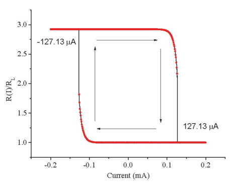
Figure 4: The transfer characteristic (or firing behavior) for a STT-based current-driven spin neuron at 0 K. $R(I)$ is the resistance of the MTJ when the total current injected into the soft layer (due to weighted inputs and bias) is $I$ and $R_{L}$ is again the low resistance of the MTJ.

First, we determine the current required to switch the soft layer (from the LLG simulations) and find it to be 127.13 $\mu$A (the corresponding current density is 10.11 MA/cm²) for a current pulse of duration 10 ns. Ref. [44] also assumed a current pulse duration of 10 ns and found the switching current density to be 4 MA/cm² for a barrier height of 42 kT in perpendicular magnetic anisotropy (our barrier height is 71.7 kT). Ref. [45] considered a CoFeB soft nanomagnet with in-plane anisotropy barrier of $\sim$57 kT (calculated from the reported dimensions of 170 nm $\times$ 60 nm $\times$ 1.4 nm using Ref. [28]) and found the switching current density to be $\sim$ 5.5 MA/cm² for a switching time of 10 ns.

Figure 4 shows the 0 K temperature transfer characteristic (or firing behavior) of the MTJ when the total input current $I$ has been varied between -200 $\mu$A and +200 $\mu$A. Note that rounded corners are more “square” here because a subthreshold current (unlike subthreshold voltage) hardly rotates the magnetization of the soft magnet and hence does not alter the MTJ resistance perceptibly.

If we consider a typical resistance-area product (RA) of 2.1 $\Omega$-$\mu$m² for the MTJ in the high resistance state [46] and a TMR ratio of 200%, then the high-state MTJ resistance for our chosen dimensions becomes 1671 ohms and the low-state MTJ resistance 557 ohms. Energy dissipation $E_{R}$ due to the current passing through MTJ’s tri-layered structure is given by [47]

$$E_{R}=\int_{0}^{\tau}dtI^{2}\left[R_{P}+(R_{AP}-R_{P})\left(\frac{1-\cos{\theta(t)}}{2}\right)\right],$$ (14)

where $R_{P}$ and $R_{AP}$ are the MTJ resistances in the parallel (low) and anti-parallel (high) state, and $\theta(t)$ is the angle between the magnetization states of the soft layer and the hard layer at time $t$. This dissipation turns out to be $\sim$0.26 pJ. The LLG simulation showed that the neuron takes 14 ns to switch. The dissipation due to Gilbert damping in the soft magnet is a mere $\sim$0.48 aJ, which is negligible.

The total dissipation reported in Ref. [8] for current-driven spin neurons that use magnets with perpendicular anisotropy is 0.4 fJ. We used magnets with in-plane anisotropy. There are at least two reasons why Ref. [8] could have reported a 650 times lower dissipation compared to what we found (0.26 pJ). First, their critical current density was 4 MA/cm² which is 2.5 times less than ours. Presumably, the lower current density is due to the fact that the energy barrier between stable magnetization states in their device might have been only $\sim$40 kT which is what we estimate following the procedure in Refs. [48] and [36]. Ours was 71.7 kT. The critical current density scales with the energy barrier height; for example, Ref. [49] reported a critical current density of 8.7 MA/cm² for a barrier height of 67 kT. Additionally, in Ref. [8], the soft layer thickness was only 2 nm to maintain perpendicular anisotropy, whereas our thickness was 5 nm and the critical current density increases with the soft layer thickness [42]. These two factors increased the current density in our case and caused a higher dissipation. Second, and more importantly, Ref. [8] utilized the spin Hall effect to inject/extract spin polarized current from the magnets which would allow passing the charge current parallel to the heterointerface between the spacer and the magnets. This would allow the current to avoid going through the highly resistive spacer and decrease the resistance-area product of the MTJ considerably compared to ours. These two factors might be the cause for the 650 times lower dissipation figure reported in Ref. [8] compared to what we find. Even then, the lower dissipation reported in Ref. [8] is still 45 times higher than that encountered in the straintronic spin neuron. If we carry out the comparison between similar designs (in-plane anisotropy magnets, similar energy barrier heights to maintain similar resilience to thermally induced random firing), then the difference is even more stark; the straintronic spin neuron is 29445 times more energy-efficient and yet 10 times faster. The current-driven spin neuron however has however one small advantage; it has a 50% higher on/off ratio of the MTJ resistance because the angular separation between the two stable orientations of the soft magnet in the MTJ is $\sim 180^{\circ}$ for the current-driven spin neuron and $\sim 90^{\circ}$ for the straintronic spin neuron.

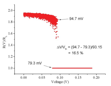
Figure 5: Transfer characteristic (or firing behavior) for the straintronic spin neuron at room temperature in the presence of thermal noise. Results are shown for positive threshold only since no additional information can be gleaned from the negative threshold segment. Since the simulation is terminated immediately upon completion of firing, no fluctuations in the transfer characteristic are visible in the low-resistance state.

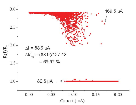
Figure 6: Transfer characteristic (or firing behavior) for the current-driven spin neuron at room temperature in the presence of thermal noise.

5 Room-temperature firing behavior of spin neurons

The room temperature firing characteristics are found by solving the stochastic LLG equation which will generate a distribution of characteristics since each one is slightly different in the presence of thermal noise. Each characteristic will show slightly different switching threshold and slightly different switching delay.

Figure 5 shows the $R(V)/R_{L}$ versus $V$ characteristic of the straintronic spin neuron at 300 K when switching from high- to low-resistance state (the characteristic for switching from low- to high-resistance state will be qualitatively similar and hence not shown). As many as 10,000 switching trajectories were simulated from the stochastic LLG equation and make up this plot. There average switching time was 0.61 ns when the voltage appearing at node $P$ in Figure 1 was above the 0 K threshold voltage of 93.15 mV. Clearly, the threshold has been significantly broadened at room temperature, indicating that there is a significant probability of pre-mature firing (firing before reaching the threshold defined at 0K) because of random thermal torque, as well as failure to fire at or slightly beyond the threshold for the same reason. The likelihood of false firing is a matter of concern which calls for further investigation of thermal degradation.

One measure of the threshold broadening is the ratio $\Delta V$/$V_{th}$, where $V_{th}$ is the average voltage at which the neuron fires and $\Delta V$ is the standard deviation. For the straintronic spin neuron studied, this quantity turns out to be 16.5%. Of course this can be reduced by increasing $V_{th}$ (by making the soft nanomagnet more shape-anisotropic to increase the in-plane shape anisotropy energy), but this will also increase the energy dissipation which varies roughly as $V_{th}^{2}$ (because the dissipation is dominated by the $CV^{2}$ loss). Let us say that 1% broadening is acceptable. Then we will have to increase $V_{th}$ 16.5-fold (assuming that it does not change $\Delta V$), resulting in an energy dissipation of 8.83aJ $\times$ 16.5² = 2.4 fJ. This is still much less than what is encountered in CMOS-base implementations (0.7 pJ reported in Ref. [8]).

The same thermal broadening is not only present in a current-driven spin neuron, but it is much worse there. Figure 6 shows $R(I)/R_{L}$ versus $I$ for the current-driven spin neuron where $I$ is the driving current. Here, 5,000 switching trajectories were simulated to produce this plot because simulation of 10,000 trajectories became computationally prohibitive (because of the longer simulation time). The average switching time was now 7.26 ns above the 0 K threshold current of 127.13 $\mu$A. The quantity $\Delta I$/$I_{th}$ turns out to be 69.92% for the simulated neuron. Had we been able to simulate more trajectories, we might have found the broadening to be even worse. Once again, the relative broadening can be reduced by increasing $I_{th}$ (by increasing the shape anisotropy of the soft nanomagnet) but of course at the cost of increasing dissipation since the latter varies roughly as $I_{th}^{2}$ (because the dissipation is dominated by the $I^{2}R$ loss). Once again, if 1% broadening is acceptable, then we will need to increase the threshold 69-fold (assuming this does not change $\Delta I$), resulting in an energy dissipation of 0.26pJ $\times$ 69² = 1.23 nJ. This would make it 1768 times worse than CMOS-based neurons and therefore the viability of STT-based spin neurons at room temperature is questionable. Even if better design (use of spin Hall effect, perpendicular anisotropy magnets, etc.) can reduce the energy dissipation by two orders of magnitude, it will still provide little advantage over CMOS implementations. In contrast, the straintronic spin neuron is still $\sim$290 times more energy-efficient than its CMOS-based counterpart at room temperature.

6 Conclusion

In conclusion, we have proposed and analyzed a straintronic spin-neuron that is orders of magnitude more energy-efficient than the usual current-driven spin neuron and also faster. The primary obstacle they both face is the significant broadening of the firing threshold at room temperature. For the current-driven spin neuron, it may not be possible to mitigate this problem without increasing the energy dissipation to the point where it is no longer superior to CMOS-based implementations. Fortunately, for the straintronic spin neuron, it may still be possible to mitigate this problem while retaining a significant energy advantage over CMOS.

7 Appendix

The broadening in Fig. 6 for current-driven spin neuron due to thermal noise at room temperature can be reduced if we choose a different soft material with larger Gilbert damping coefficient ($\alpha$). Since the switching current density is approximately linearly proportional to $\alpha$, the energy dissipation will increase quadratically. In order to illustrate this, we chose a hypothetical material which is identical to CoFeB in all respects, except its Gilbert damping coefficient $\alpha$ is 0.1 and carried out the stochastic LLG simulations. The switching current turned out to be 1.44 mA for a current pulse duration of 10 ns, but the broadening ($\Delta$I/I_th) was reduced to 11.25%. However, the extremely large switching current results in energy dissipation of 23.8 pJ which is clearly prohibitive. This case study shows us that although thermal degradation may be countered with increased energy dissipation, the price to be paid in energy may be prohibitive.

Programmable synapses: In this paper, our synapses have fixed weights because they are implemented with passive resistors. Programmable synapses are required for more versatile renditions of neural computing such as Spike Time Dependent Plasticity (STDP) models of neural networks [50, 51, 52, 53] that are popular for Hebbian learning [54]. For STDP models, the synapse weight should be programmed by a spike signal, e.g. it should be a function of a time-integrated spike current. The time integrated spike current is a charge that could be stored in a capacitor which then applies a voltage across a piezoelectric layer that generates strain and rotates the magnetization of a magnetostrictive magnet that is elastically coupled to the piezoelectric layer. The magnetostrictive magnet could be the soft layer of a magneto-tunneling junction whose resistance is thus programmed by the time integrated spike signal, resulting in the appropriate programmable synapse. This is a different topic and would be treated elsewhere.

This work was supported by the US National Science Foundation under grants ECCS-1124714 and CCF-1216614. J. A. would also like to acknowledge the NSF CAREER grant CCF-1253370.

References

References

- [1] L. Chua and L. Yang, Cellular neural networks: applications, IEEE Trans. Circuits Syst. 35, 1273 (1988).
- [2] M. Ueda, Y. Kaneko, Y. Nishitani, and E. Fujii, A neural network circuit using persistent interfacial conducting heterostructures, J. Appl. Phys. 110, 086104 (2011).
- [3] P. Simard, D. Steinkraus, and J. C. Platt, Best practices for convolutional neural networks applied to visual document analysis, in proceedings of the International Conference on Document Analysis and Recognition (ICDAR) 3, 958 (2003).
- [4] D. George and J. Hawkins, Towards a mathematical theory of cortical micro-circuits, PLOS Comput. Biol. 5, e1000532 (2009).
- [5] R. Lippmann, An introduction to computing with neural nets, IEEE ASSP Mag. 2, 4 (1987).
- [6] S. Datta, S. Salahuddin, and B. Behin-Aein, Non-volatile spin switch for boolean and non-boolean logic, Appl. Phys. Lett. 101, 252411 (2012).
- [7] M. Sharad, C. Augustine, G. Panagopoulos, and K. Roy, Spin-based neuron model with domain-wall magnets as synapse, IEEE Trans. Nanotech. 11, 843 (2012).
- [8] M. Sharad, D. Fan, and K. Roy, Spin-neurons: A possible path to energy-efficient neuromorphic computers, J. Appl. Phys. 114, 234906 (2013).
- [9] L. Liu, C.-F. Pai, Y. Li, H. W. Tseng, D. C. Ralph, and R. A. Buhrman, Spin-torque switching with the giant spin hall effect of tantalum, Science 336, 555 (2012).
- [10] F. Zavaliche, T. Zhao, H. Zheng, F. Straub, M. P. Cruz, P.-L. Yang, D. Hao, and R. Ramesh, Electrically assisted magnetic recording in multiferroic nanostructures, Nano Lett. 7, 1586 (2007).
- [11] T. Brintlinger, S.-H. Lim, K. H. Baloch, P. Alexander, Y. Qi, J. Barry, J. Melngailis, L. Salamanca-Riba, I. Takeuchi, and J. Cumings, In situ observation of reversible nanomagnetic switching induced by electric fields, Nano Lett. 10, 1219 (2010).
- [12] J. Atulasimha and S. Bandyopadhyay, Bennett clocking of nanomagnetic logic using multiferroic single domain nanomagnets, Appl. Phys. Lett. 97, 173105 (2010).
- [13] M. Buzzi, R. Chopdekar, J. L. Hockel, A. Bur, T. Wu, N. Pilet, P. Warnicke, G. P. Carman, L. J. Heyderman, and F. Nolting, Single domain spin manipulation by electric fields in strain coupled artificial multiferroic nanostructures, Phys. Rev. Lett. 111, 027204 (2013).
- [14] N. D Souza, M. Salehi-Fashami, S. Bandyopadhyay, and J. Atulasimha, Strain induced clocking of nanomagnets for ultra low power boolean logic, arXiv:1404.2980 [cond-mat.mes-hall] (2014).
- [15] N. Tiercelin, Y. Dusch, V. Preobrazhensky, and P. Pernod, Magnetoelectric memory using orthogonal magnetization states and magnetoelastic switching, J. Appl. Phys. 109, 07D726 (2011).
- [16] N. A. Pertsev and H. Kohlstedt, Magnetic tunnel junction on a ferroelectric substrate, Appl. Phys. Lett. 95, 163503 (2009).
- [17] K. Roy, S. Bandyopadhyay, and J. Atulasimha, Binary switching in a symmetric potential landscape, Sci. Rep. 03, 3038 (2013).
- [18] A. K. Biswas, S. Bandyopadhyay, and J. Atulasimha, Energy-efficient magnetoelastic non-volatile memory, Appl. Phys. Lett. 104, 232403 (2014).
- [19] A. K. Biswas, S. Bandyopadhyay, and J. Atulasimha, Complete magnetization reversal in a magnetostrictive nanomagnet with voltage generated stress: A reliable energy-efficient non-volatile magnetoelastic memory, Appl. Phys. Lett. 105, 072408 (2014).
- [20] J. J. Wang, J. M. Hu, J.Ma, J. X. Zhang, L. Q. Chen, and C. W. Nan, Full 180∘ magnetization reversal with electric fields, Sci. Rep. 04, 7507 (2014).
- [21] M. S. Fashami, K. Roy, J. Atulasimha, and S. Bandyopadhyay, Magnetization dynamics, bennett clocking and associated energy dissipation in multiferroic logic, Nanotechnology 22, 155201 (2011).
- [22] M. S. Fashami, J. Atulasimha, and S. Bandyopadhyay, Magnetization dynamics, throughput and energy dissipation in a universal multiferroic nanomagnetic logic gate with fan-in and fan-out, Nanotechnology 23, 105201 (2012).
- [23] A. K. Biswas, J. Atulasimha, and S. Bandyopadhyay, An error-resilient non-volatile magneto-elastic universal logic gate with ultralow energy-delay product, Sci. Rep. 4, 7553 (2014).
- [24] G. Salis, R. Wang, X. Jiang, R. M. Shelby, S. S. P. Parkin, S. R. Bank, and J. S. Harris, Temperature independence of the spin-injection efficiency of a MgO-based tunnel spin injector, Appl. Phys. Lett. 87, 262503 (2005).
- [25] S. Ikeda, J. Hayakawa, Y. Ashizawa, Y. M. Lee, K. Miura, H. Hasegawa, M. Tsunoda, F. Matsukura, and H. Ohno, Tunnel magnetoresistance of 604% at 300 K by suppression of Ta diffusion in CoFeB/MgO/CoFeB pseudo-spin-valves annealed at high temperature, Appl. Phys. Lett. 93, 082508 (2008).
- [26] J. Cui, J. L. Hockel, P. K. Nordeen, D. M. Pisani, C. y. Liang, G. P. Carman, and C. S. Lynch, A method to control magnetism in individual strain-mediated magnetoelectric islands, Appl. Phys. Lett. 103, 232905 (2013).
- [27] R. P. Cowburn, D. K. Koltsov, A. O. Adeyeye, M. E. Welland, and D. M.Tricker, Single-domain circular nanomagnets, Phys. Rev. Lett. 83, 1042 (1999).
- [28] M. Beleggia, M. D. Graef, Y. T. Millev, D. A. Goode, and G. Rowlands, Demagnetization factors for elliptic cylinders, J. Phys. D: Appl. Phys. 38, 3333 (2005).
- [29] K. Roy, S. Bandyopadhyay, and J. Atulasimha, Energy dissipation and switching delay in stress-induced switching of multiferroic nanomagnets in the presence of thermal fluctuations, J. Appl. Phys. 112, 023914 (2012).
- [30] W. Scholz, T. Schrefl, and J. Fidler, Micromagnetic simulation of thermally activated switching in fine particles, J. Magn. Magn. Mater. 233, 296 (2001).
- [31] R. Abbundi and A. E. Clark, Anomalous thermal expansion and manetostriction of single crystal Tb0.27Dy0.73Fe2, IEEE Trans. Magn. 13, 1519 (1977).
- [32] K. Ried, M. Schnell, F. Schatz, M. Hirscher, B. Ludescher, W. Sigle, and H. Kronmller, Crystallization behaviour and magnetic properties of magnetostrictive TbDyFe films, Phys. Status Solidi A 167, 195 (1998).
- [33] R. Kellogg and A. Flatau, Experimental investigation of Terfenol-D s elastic modulus, J. Intell. Mater. Syst. Struct. 19, 583 (2008).
- [34] T. V. Lyutyy, S. I. Denisov, A. Y. Peletskyi, and C. Binns, Energy dissipation in single-domain ferromagnetic nanoparticles: Dynamical approach, arXiv:1502.04222v1[cond-mat.mes-hall] (2015).
- [35] S. Iihama, S. Mizukami, H. Naganuma, M. Oogane, Y. Ando, and T. Miyazaki, Gilbert damping constants of Ta/CoFeB/MgO(Ta) thin films measured by optical detection of precessional magnetization dynamics, Phys. Rev. B 89, 174416 (2014).
- [36] S. Ikeda, K. Miura, H. Yamamoto, K. Mizunuma, H. D. Gan, M. Endo, S. Kanai, J. Hayakawa, F. Matsukura, and H. Ohno, A perpendicular-anisotropy CoFeB-MgO magnetic tunnel junction, Nature Mater. 9, 721 (2010).
- [37] M. Sharad, D. Fan, K. Aitken, and K. Roy, Energy-efficient non-boolean computing with spin neurons and resistive memory, IEEE Trans. Nanotech. 13, 23 (2014).
- [38] J. Slonczewski, Current-driven excitation of magnetic multilayers, J. Magn. Magn. Mater. 159, L1 (1996).
- [39] D. C. Ralph and M. D. Stiles, Spin transfer torques, J. Magn. Magn. Mater. 320, 1190 (2008).
- [40] H. Kubota, A. Fukushima, K. Yakushiji, T. Nagahama, S. Yuasa, K. Ando, H. Maehara, Y. Nagamine, K. Tsunekawa, D. D. Djayaprawira, N. Watanabe, and Y. Suzuki, Quantitative measurement of voltage dependence of spin-transfer torque in MgO-based magnetic tunnel junctions, Nature Phys. 4, 37 (2008).
- [41] G. E. Rowlands, T. Rahman, J. A. Katine, J. Langer, A. Lyle, H. Zhao, J. G. Alzate, A. A. Kovalev, Y. Tserkovnyak, Z. M. Zeng, H. W. Jiang, K. Galatsis, Y. M. Huai, P. K. Amiri, K. L. Wang, I. N. Krivorotov, and J.-P. Wang, Deep subnanosecond spin torque switching in magnetic tunnel junctions with combined in-plane and perpendicular polarizers, Appl. Phys. Lett. 98, 102509 (2011).
- [42] J. Hayakawa, S. Ikeda, Y. M. Lee, R. Sasaki, T. Meguro, F. Matsukura, H. Takahashi, and H. Ohno, Current-driven magnetization switching in CoFeB/MgO/CoFeB magnetic tunnel junctions, Jap. J. Appl. Phys. 44, L1267 (2005).
- [43] S. Salahuddin, D. Datta, and S. Datta, Spin transfer torque as a non-conservative pseudo-field, arXiv:0811.3472 [cond-mat.mes-hall] (2008).
- [44] P. K. Amiri, Z. M. Zeng, J. Langer, H. Zhao, G. Rowlands, Y.-J. Chen, I. N. Krivorotov, J.-P. Wang, H. W. Jiang, J. A. Katine, Y. Huai, K. Galatsis, and K. L. Wang, Switching current reduction using perpendicular anisotropy in CoFeB/MgO magnetic tunnel junctions, Appl. Phys. Lett. 98, 112507 (2011).
- [45] R. Tomasello, V. Puliafito, B. Azzerboni, and G. Finocchio, Switching properties in magnetic tunnel junctions with interfacial perpendicular anisotropy: Micromagnetic study, IEEE Trans. Magn. 50, 7100305 (2014).
- [46] S. Isogami, M. Tsunoda, K. Komagaki, K. Sunaga, Y. Uehara, M. Sato, T. Miyajima, and M. Takahashi, In situ heat treatment of ultrathin mgo layer for giant magnetoresistance ratio with low resistance area product in CoFeB/MgO/CoFeB magnetic tunnel junctions, Appl. Phys. Lett. 93, 192109 (2008).
- [47] M. Carpentieri, M. Ricci, P. Burrascano, L. Torres, and G. Finocchio, Wideband microwave signal to trigger fast switching processes in magnetic tunnel junctions, J. Appl. Phys. 111, 07C909 (2012).
- [48] K. Lee, J. J. Sapan, S. H. Kang, and E. E. Fullerton, Perpendicular magnetization of CoFeB on single crystal MgO, J. Appl. Phys. 109, 123910 (2011).
- [49] S. Ikeda, J. Hayakawa, Y. M. Lee, F. Matsukura, H. Ohno, and T. Hanyu, Magnetic tunnel junctions for spintronic memories and beyond, IEEE Trans. Elec. Dev. 54, 991 (2007).
- [50] G-q Bi and M-m Poo, Synaptic modifications in cultured hippocampal neurons: Dependence on spike timing, synaptic strength, and postsynaptic cell type, J. Neuroscience 18, 10464 (1998).
- [51] M. Favero, A. Cangiano and G. Busetto, Hebb-based rules of neuro-plasticity: Are they ubiquitously important for the refinement of synaptic connections in development, The Neuroscientist 20, 8 (2014).
- [52] T. Aoki and T. Aoyagi, A possible role of incoming spike synchrony in associative memeory model with STDP learning rule, Prog. Theor. Phys. Suppl. 161, 152 (2006).
- [53] A. Sengupta, Z. Al Azim, X. Fong and K. Roy, Spin-orbit torque induced spike-timing dependent plasticity, Appl. Phys. Lett. 106, 093704 (2015).
- [54] D. Hebb, The Organization of Behavior (Wiley, New York, 1949).