A variant of the linear isotropic indeterminate couple stress model with symmetric local force-stress, symmetric nonlocal force-stress, symmetric couple-stresses and complete traction boundary conditions

Abstract

In this paper we venture a new look at the linear isotropic indeterminate couple stress model in the general framework of second gradient elasticity and we propose a new alternative formulation which obeys Cauchy-Boltzmann’s axiom of the symmetry of the force stress tensor. For this model we prove the existence of solutions for the equilibrium problem. Relations with other gradient elastic theories and the possibility to switch from a 4th order (gradient elastic) problem to a 2nd order micromorphic model are also discussed with a view of obtaining symmetric force-stress tensors. It is shown that the indeterminate couple stress model can be written entirely with symmetric force-stress and symmetric couple-stress. The difference of the alternative models rests in specifying traction boundary conditions of either rotational type or strain type. If rotational type boundary conditions are used in the partial integration, the classical anti-symmetric nonlocal force stress tensor formulation is obtained. Otherwise, the difference in both formulations is only a divergence–free second order stress field such that the field equations are the same, but the traction boundary conditions are different. For these results we employ a novel integrability condition, connecting the infinitesimal continuum rotation and the infinitesimal continuum strain. Moreover, we provide the complete, consistent traction boundary conditions for both models.

Key words: symmetric Cauchy stresses, generalized continua, non-polar material, microstructure, size effects, microstrain model, non-smooth solutions, gradient elasticity, strain gradient elasticity, couple stresses, polar continua, hyperstresses, Boltzman axiom, dipolar gradient model, modified couple stress model, conformal invariance, micro-randomness, symmetry of couple stress tensor, consistent traction boundary conditions.

AMS 2010 subject classification: 74A30, 74A35.

Dedicated to Richard Toupin, in deep admiration of his scientific achievements.

1 Introduction

1.1 General viewpoint

The Cosserat model is an extended continuum model which features independent degrees of rotation in addition to the standard translational degrees of particles, see [28, 83, 81, 66, 64] for a detailed exposition. The prize, which has to be paid for this extension are non-symmetric force stress tensors together with so-called couple stress tensors which then represent the response of the model due to spatially differing Cosserat rotations. The couple stress model is the Cosserat model [48] with restricted rotations, i.e. in which the Cosserat rotations coincide with the continuum rotations. As such it belongs also to a certain subclass of gradient elasticity models, where the higher derivatives only act on the continuum rotations. This constitutes a big conceptual advantage since the interpretation of the Cosserat rotations as new physical degrees of freedom is in general a difficult task. Such a model is also called a model with “latent microstructure” [11, 12].

Let $F=R\,U$ be the polar decomposition of the deformation gradient $F=\nabla\varphi$ into rotation $R\in{\rm SO}(3)$ and positive definite symmetric right stretch tensor $U=\sqrt{F^{T}F}$, where $\varphi:\Omega\subset\mathbb{R}^{3}\rightarrow\mathbb{R}^{3}$ characterizes the deformation of the material filling the domain $\Omega\subseteq\mathbb{R}^{3}$. We write $R={\rm polar}(F)$. In a variational context, the energy density $W$ to be minimized in the geometrically nonlinear constrained Cosserat model is given by

$$W=W(\underbrace{U-{\boldsymbol{\mathbbm{1}}}}_{\text{strain}},\underbrace{{\rm polar}(F)^{T}\nabla_{\rm x}{\rm polar}(F)}_{\text{curvature}})\,,$$ (1.1)

which reduced form follows from left-invariance of the Lagrangian $W$ under superposed rotations. In this paper, our objectives are much more modest. We will only be concerned with the linearized variant of (1.1), which can be written as

$$W=W(\!\!\!\!\!\!\underbrace{\operatorname{sym}\nabla u}_{\begin{array}[]{c}\text{\footnotesize{infinitesimal}}\vspace{-1.5mm}\\ \text{\footnotesize{strain}}\end{array}}\!\!\!\!\!\!,\,\underbrace{\nabla[\operatorname{axl}(\text{skew}\nabla u)]}_{\begin{array}[]{c}\text{\footnotesize{infinitesimal}}\vspace{-1.5mm}\\ \text{\footnotesize{curvature}}\end{array}})=W_{\rm lin}(\operatorname{sym}\nabla u)+W_{\rm curv}(\nabla[\operatorname{axl}(\text{skew}\nabla u)]),$$ (1.6)

where $u:\Omega\subset\mathbb{R}^{3}\rightarrow\mathbb{R}^{3}$ is the displacement and

$$\nabla\operatorname{axl}(\text{skew}\nabla u)=2\,\textrm{curl\,}u.$$ (1.7)

The energy density (1.6) is the classical Lagrangian for the indeterminate couple stress formulation. As will be seen later, this formulation leads naturally to totally skew symmetric nonlocal force stress contributions.

Toupin already remarked on an alternative representation of the energy (1.1) [102, Section 6] which leads, in its linearized variant given by Mindlin [72, eq. (2.4)] to a dependence on

$$W=W(\operatorname{sym}\nabla u,\operatorname{Curl\,}(\operatorname{sym}\nabla u))=W_{\rm lin}(\operatorname{sym}\nabla u)+W_{\rm curv}(\operatorname{Curl\,}(\operatorname{sym}\nabla u))\,,$$ (1.8)

due to the equivalence

$$\nabla(\operatorname{axl}\text{skew}\nabla u)=\frac{1}{2}\nabla\textrm{curl\,}u=(\operatorname{Curl\,}(\operatorname{sym}\nabla u))^{T}$$

instead of (1.6). The representation $\frac{1}{2}\nabla\textrm{curl\,}u$ is directly derived from the original Cosserat model [15, 98]. Both authors, Toupin and Mindlin, noted that now, comparing (1.6) and (1.8) the force stress tensors and the couple stress tensors are changed while the balance of linear momentum equation remains unchanged such that these concepts are not uniquely defined (see also Truesdell and Toupin’s remark on null-tensors [105, p.  547]. However, they apparently did not realize that it is possible to use this ambiguity to obtain completely symmetric force stress tensors also in the couple stress model which is otherwise the paragon for a model having non-symmetric force stress tensors. We also need to remark that in a purely mechanical context, the observation of size-effects does not necessitate to introduce skew-symmetric stress-tensors [5].

In this paper we do not discuss in detail the field of applications of such a special format of gradient elasticity model. Suffice it to say that much attention is directed to nano-scaled material in which size-effects may become important, which may make the present model applicable at strong stress gradients in the vicinity of cracks, or more generally, in highly heterogeneous media. We must also warn the reader: the indeterminate couple stress model is, in our view, a certain singular limit of the Cosserat model with independent displacements and micro-rotation and therefore some degenerate behaviour is to be expected throughout.

1.2 The linear indeterminate couple stress model

As hinted at above, the indeterminate couple stress model is a specific gradient elastic model in which the higher order interaction is restricted to the continuum rotation $\text{skew}\,\nabla u$ (or equivalently, $\textrm{curl\,}u$). It is therefore traditionally interpreted to include interactions of rotating particles and it is possible to prescribe boundary conditions of rotational type. Superficially, this is the simplest possible generalization of linear elasticity in order to include the gradient of the local continuum rotation as a source of stress and strain energy. In this paper, we limit our analysis to linear isotropic materials and only to the second gradient of the displacement

$$D^{2}u=u_{k,ij}=\varepsilon_{ik,j}-\varepsilon_{jk,i}-\varepsilon_{ij,k},\quad\text{where}\quad\varepsilon=\operatorname{sym}\nabla u.$$

In general, the strain gradient models have the great advantage of simplicity and physical transparency since there are no new independent degree of freedoms introduced which would require interpretation. Since in this model there are no additional degrees of freedom (as compared to the Cosserat or micromorphic approach) the higher derivatives introduce a “latent-microstructure” (constrained microstructure). However, this apparent simplicity has to be payed with much more complicated traction boundary conditions, as will be seen later.

We will see in Section 4, surprisingly, that the mentioned rotational interaction can equivalently be viewed as a strain type interaction in the indeterminate couple stress model. Therefore, the first interpretation of rotational interaction (which is classical) is ambiguous as long as the problem is not specified together with boundary conditions appearing as effect of the kind of partial integration which is performed. We may choose, contrarily to our intuition, another representation of the curvature energy motivated by formal considerations of invariance properties. In this regard we highlight the fact that force stresses for a material of higher order are far from being uniquely defined: it is always possible to add a self-equilibrated (divergence-free tensor field) force field changing the constitutive stress tensor but leaving unaltered the equilibrium equations [26, 73].

Often, such kind of models introduce too many additional parameters (or too many additional artificial degrees of freedom) which are neither easily interpreted, nor easily to be determined from experiments. Our discussion may also be interpreted with the background to only include those higher order terms that are required to describe the pertinent physics. It is clear that higher order models should not be more complicated than is warranted by experimental observation. A permanent nuisance in this respect is the question of how to identify new material parameters which are connected to the possible non-symmetry of the total force-stress tensor having the same dimensions as the classical shear modulus $\mu$ ${\rm[N/mm^{2}]}$. In the Cosserat model the connecting parameter is the Cosserat-couple modulus $\mu_{c}$ [28, 82], which, for the indeterminate couple stress model considered here, is formally $\mu_{c}\rightarrow\infty$.

The Cauchy-Boltzmann axiom, well known from classical elasticity, requires the symmetry of the force stress tensor and may serve us also in the realm of this higher order theory to restrict the bewildering possibilities. Already Cauchy wrote [13, p. 344-345]:

“… les composantes $\mathcal{A},\mathcal{F},\mathcal{E};\mathcal{F},\mathcal{B},\mathcal{D};\mathcal{E},\mathcal{D},\mathcal{C}$ des pressions supportées au point P par trois plans parallèles aux plans coordonnés des $yz$, des $zx$ et des $xy$, pourront être généralement considérées comme des fonctions linéaires des déplacements $\xi,\eta,\zeta$ et des leurs dérivées des divers ordres.”.

Truesdell and Toupin [105, p. 390] write:

““Theories of elastic materials of grade 2 or higher had been proposed by several authors [Cauchy [13], St. Venant [97], Jaramillo [47]], but under the assumption that the [total-force] stress tensor is symmetric”.

Indeed, Jaramillo [47] considers a second gradient elastic material and obtains the dynamic equations by Hamilton’s principle. He observes dispersion relations in wave propagation problems. For simplicity only he restricts his discussion to those second gradient formulations, which give rise to a symmetric total force-stress tensor and obtains a classification for isotropic materials [47, p. 51, Eq. (96)]. The subject was pushed forward in the late 1950’s with works of Toupin [102, 103], Grioli [37, 38], Mindlin  [69] and Koiter [51], among others, see the references later in this paper. Yang et al. [106] give an erroneous motivation for a symmetric moment stress tensor, as will be shown in [74]. Neff et al. [85] considered the singular stiffening behaviour for arbitrary small samples in the Cosserat and indeterminate couple stress model and concluded that in order to avoid these singular effects one has to take a symmetric moment stress, thus providing the first rational argument in favour of symmetric moment stresses. In [85] the same model has been derived based on a homogenization procedure and a novel invariance requirement introduced by Neff et al. [48], called micro-randomness and it has been shown that the model is well-posed.

1.3 Our perspective

Our contribution is intended to clarify and delineate under what boundary conditions we may expect or use symmetric nonlocal force stresses in the indeterminate couple stress model. When trying to relax the 4.th order problem (from gradient elasticity), it also seems expedient to retain the symmetry of the force stress tensor and of the moment stress tensor. Respecting symmetry restricts the possibilities to choose among 2.nd order micromorphic models. The importance of switching to a 2.nd order problem with new independent degrees of freedom is clear from the implementational point of view with finite elements: a 2.nd order problem is much easier and more efficient. However, given the antisymmetric classical and our new symmetric formulations we may arrive at completely different 2.nd order formulations in case of mixed displacement-traction boundary conditions.

In general, the hyperstress-tensor (couple stresses, sometimes called double-stress [65]) in second gradient elasticity [102, 69, 51, 100, 16, 17] (see also the recent papers [20, 21, 19, 107, 95, 6, 18, 29, 59, 27, 94, 25]) may be defined as $\mathfrak{m}=(\mathfrak{m}_{ijk})=D_{D^{2}u}W(D^{2}u)$. Since $D^{2}u=(u_{i,jk})$ is a third order tensor, so is $\mathfrak{m}$. Moreover, since $u_{i,jk}$ is symmetric in $(jk)$ the same is usually assumed for $\mathfrak{m}_{ijk}$. This, however, is not mandatory, see [73].

In the framework considered in this paper, the hyperstress-tensor is defined as

$$\widetilde{m}:=D_{\nabla(\textrm{curl\,}u)}W_{\rm curv}(\nabla(\textrm{curl\,}u))\qquad\ \text{ or }\qquad\ \widehat{m}:=D_{\operatorname{Curl\,}(\operatorname{sym}\nabla u)}W_{\rm curv}(\operatorname{Curl\,}(\operatorname{sym}\nabla u)),$$

respectively, and both expressions are 2.nd order tensors and are also called couple stress tensors, since they act as dual objects to gradients of rotations. On the other hand, as we will see, we have two competing expressions of the nonlocal force stress tensor: a symmetric tensor $\widehat{\tau}$ versus an anti-symmetric tensor $\widetilde{\tau}$:

$$\widehat{\tau} =\mu\,L_{c}^{2}\,\operatorname{sym}\operatorname{Curl\,}\{2\,\alpha_{1}\operatorname{dev}\operatorname{sym}\operatorname{Curl\,}(\operatorname{sym}\nabla u)+2\,\alpha_{2}\,\operatorname{skew}\operatorname{Curl\,}(\operatorname{sym}\nabla u)\}=\operatorname{sym}\operatorname{Curl\,}(\widehat{m})\in{\rm Sym}(3)$$

$$\widetilde{\tau} =\frac{\mu}{2}\,L_{c}^{2}\,\operatorname{anti}{\rm Div}\{2\,\alpha_{1}\,\operatorname{dev}\operatorname{sym}\nabla[\operatorname{axl}(\operatorname{skew}\nabla u)]+2\,\alpha_{2}\,\operatorname{skew}\nabla[\operatorname{axl}(\operatorname{skew}\nabla u)]\}=\frac{1}{2}\operatorname{anti}{\rm Div}(\widetilde{m})\in\operatorname{\mathfrak{so}}(3),$$

with ${\rm Div}(\widehat{\tau}-\widetilde{\tau})=0$. Since $[\operatorname{Curl\,}(\operatorname{sym}\nabla u)]^{T}=\nabla[\operatorname{axl}(\operatorname{skew}\nabla u)]$, it follows

$$\widehat{\tau}-\widetilde{\tau}=\mu\,L_{c}^{2}\,\Big{\{} \quad\ 2\,\alpha_{1}\,(\operatorname{sym}\operatorname{Curl\,}-\frac{1}{2}\,\operatorname{anti}{\rm Div}).[\operatorname{dev}\operatorname{sym}\operatorname{Curl\,}(\operatorname{sym}\nabla u)]$$

$$\,+2\,\alpha_{2}\,(\operatorname{sym}\operatorname{Curl\,}+\frac{1}{2}\operatorname{anti}{\rm Div}).[\operatorname{skew}\operatorname{Curl\,}(\operatorname{sym}\nabla u)]\quad\ \ \Big{\}}.$$

The independent constitutive variable $\widetilde{k}:=\nabla(\textrm{curl\,}u)$ is the second gradient contribution considered by Grioli [37], Toupin [102], Mindlin [72], Koiter [51] and Sokolowski [100]. In general, neither $\widetilde{m}$ nor $\widehat{m}$ couple stress tensors are symmetric.

The symmetry of the force stress tensor in continuum mechanics is regulary discussed in the literature, see e.g. [52, 68, 76]. It has been suggested by McLennan [68] that a symmetric force stress tensor can always be constructed by adding divergence-free couple stresses, since only its divergence occurs in the local conservation law. However, all of the previously given expositions use anti-symmetric nonlocal force-stresses. Since there is no conclusive evidence for the real need of a non-symmetric total force-stress tensor in the purely mechanical context, we apply Ockham’s razor and discard these non-symmetric force stress formulations. Our new alternative formulation will have symmetric couple stresses and symmetric force stresses. Thus it satisfies the Cauchy-Boltzmann’s axiom. We also show that the new formulation is well-posed in statics. While conceptually very pleasing, the real merits of such a “completely symmetric” formulation have yet to be discovered.

Similarly to the classical indeterminate couple stress model which can be obtained as a constrained Cosserat model, our new $\operatorname{Curl\,}(\operatorname{sym}\nabla u)$-model can be obtained as a constrained “microstrain” model [34, 33, 78].

The question of boundary conditions in higher gradient elasticity models has been a subject of constant attention. Bleustein has formulated the conclusive answer for general gradient elastic models involving the surface divergence operator [10]. However, the traction boundary conditions obtained by Tiersten and Bleustein in [101] with respect to the special case of the indeterminate couple stress model are incomplete. In a forthcoming paper [61] we discuss and correct the form of the traction boundary conditions considered until now in the classical indeterminate couple stress model [72, 102, 51, 85, 93, 4, 106, 92]. Here, we just provide the correct answer obtained there in the form of a summarizing box.

The plan of the paper is now as follows: after a subsection fixing the notation, we outline some related models in isotropic second gradient elasticity; we prove some auxiliary results and we discuss the invariance properties of the considered energy; we recall the classical indeterminate couple stress model with skew-symmetric nonlocal force-stress (i.e. with non symmetric total force-stress tensor); we formulate the equilibrium problem for the new isotropic gradient elasticity model with symmetric nonlocal force stress (i.e. with symmetric total force-stress tensor) and we give an existence result; we discuss the difference of the classical indeterminate couple stress model with the introduced symmetric model; paying particular attention to the boundary virtual work principle we show that these two possible formulations are applicable for different types of traction boundary conditions; we discuss the possibility to switch from a 4.th-order problem to a 2.nd order micromorphic model. All our existence results can be extended, mutatis mutandis, to first order anisotropic behaviour [59, 24, 60], i.e. considering as total energy $\langle\mathbb{C}.\,\operatorname{sym}\nabla u,\operatorname{sym}\nabla u\rangle+W_{\rm curv}(D^{2}u)$ as long as $\mathbb{C}$ is a uniformly positive definite tensor. We finish with some boxes summarizing our models and findings.

1.4 Notational agreements

In this paper, we denote by $\mathbb{R}^{3\times 3}$ the set of real $3\times 3$ second order tensors, written with capital letters. For $a,b\in\mathbb{R}^{3}$ we let $\langle{a},{b}\rangle_{\mathbb{R}^{3}}$ denote the scalar product on $\mathbb{R}^{3}$ with associated vector norm $\|{a}\|^{2}_{\mathbb{R}^{3}}=\langle{a},{a}\rangle_{\mathbb{R}^{3}}$. The standard Euclidean scalar product on $\mathbb{R}^{3\times 3}$ is given by $\langle{X},{Y}\rangle_{\mathbb{R}^{3\times 3}}=\operatorname{tr}({XY^{T}})$, and thus the Frobenius tensor norm is $\|{X}\|^{2}=\langle{X},{X}\rangle_{\mathbb{R}^{3\times 3}}$. In the following we omit the index $\mathbb{R}^{3},\mathbb{R}^{3\times 3}$. The identity tensor on $\mathbb{R}^{3\times 3}$ will be denoted by ${\boldsymbol{\mathbbm{1}}}$, so that $\operatorname{tr}({X})=\langle{X},{{\boldsymbol{\mathbbm{1}}}}\rangle$. We adopt the usual abbreviations of Lie-algebra theory, i.e., $\operatorname{\mathfrak{so}}(3):=\{X\in\mathbb{R}^{3\times 3}\;|X^{T}=-X\}$ is the Lie-algebra of skew symmetric tensors and $\operatorname{\mathfrak{sl}}(3):=\{X\in\mathbb{R}^{3\times 3}\;|\operatorname{tr}({X})=0\}$ is the Lie-algebra of traceless tensors. For all $X\in\mathbb{R}^{3\times 3}$ we set $\operatorname{sym}X=\frac{1}{2}(X^{T}+X)\in{\rm{Sym}}$, $\operatorname{skew}X=\frac{1}{2}(X-X^{T})\in\operatorname{\mathfrak{so}}(3)$ and the deviatoric part $\operatorname{dev}X=X-\frac{1}{3}\;\operatorname{tr}(X){\boldsymbol{\mathbbm{1}}}\in\operatorname{\mathfrak{sl}}(3)$ and we have the orthogonal Cartan-decomposition of the Lie-algebra $\operatorname{\mathfrak{gl}}(3)$

$$\operatorname{\mathfrak{gl}}(3) =\{\operatorname{\mathfrak{sl}}(3)\cap{\rm{Sym}}(3)\}\oplus\operatorname{\mathfrak{so}}(3)\oplus\mathbb{R}\!\cdot\!{\boldsymbol{\mathbbm{1}}},\quad X=\operatorname{dev}\operatorname{sym}X+\operatorname{skew}X+\frac{1}{3}\operatorname{tr}(X){\boldsymbol{\mathbbm{1}}}\,.$$ (1.9)

Throughout this paper (when we do not specify else) Latin subscripts take the values $1,2,3$. Typical conventions for differential operations are implied such as comma followed by a subscript to denote the partial derivative with respect to the corresponding cartesian coordinate. We also use the Einstein notation of the sum over repeated indices if not differently specified. Here, for

$$\overline{A}=\left(\begin{array}[]{ccc}0&-a_{3}&a_{2}\\ a_{3}&0&-a_{1}\\ -a_{2}&a_{1}&0\end{array}\right)\in\operatorname{\mathfrak{so}}(3)$$ (1.13)

we consider the operators $\operatorname{axl}:\operatorname{\mathfrak{so}}(3)\rightarrow\mathbb{R}^{3}$ and $\operatorname{anti}:\mathbb{R}^{3}\rightarrow\operatorname{\mathfrak{so}}(3)$ through

$$\operatorname{axl}(\overline{A}):=\left(a_{1},a_{2},a_{3}\right)^{T},\quad\quad\overline{A}.\,v=(\operatorname{axl}\overline{A})\times v,\qquad\qquad(\operatorname{anti}(v))_{ij}=-\varepsilon_{ijk}v_{k},\quad\quad\forall\,v\in\mathbb{R}^{3},$$ (1.14)

$$(\operatorname{axl}\overline{A})_{k}=-\frac{1}{2}\,\epsilon_{ijk}\overline{A}_{ij}=\frac{1}{2}\,\epsilon_{kij}\overline{A}_{ji}\,,\quad\qquad\overline{A}_{ij}=-\epsilon_{ijk}(\operatorname{axl}\overline{A})_{k}=:\operatorname{anti}(\operatorname{axl}\overline{A})_{ij},\quad\quad$$

where $\epsilon_{ijk}$ is the totally antisymmetric third order permutation tensor. We recall that for a third order tensor $\mathbb{E}$ and $X\in\mathbb{R}^{3\times 3}$, $v\in\mathbb{R}^{3}$ we have the contraction operations $\mathbb{E}:X\in\mathbb{R}^{3}$, $\mathbb{E}.\,v\in\mathbb{R}^{3\times 3}$ and $X.\,v\in\mathbb{R}^{3}$, with the components

$$(\mathbb{E}:\,X)_{i}=\mathbb{E}_{ijk}\,X_{kj}\,,\qquad(\mathbb{E}.\,v)_{ij}=\mathbb{E}_{ijk}\,v_{k}\,,\qquad(X.\,v)_{i}=X_{ij}\,v_{j}.$$ (1.15)

For multiplication of two matrices we will not use other specific notations.

We consider a body which occupies a bounded open set $\Omega$ of the three-dimensional Euclidian space $\mathbb{R}^{3}$ and assume that its boundary $\partial\Omega$ is a piecewise smooth surface. An elastic material fills the domain $\Omega\subseteq\mathbb{R}^{3}$ and we refer the motion of the body to rectangular axes $Ox_{i}$. By $C_{0}^{\infty}(\Omega)$ we denote the set of infinitely differentiable functions with compact support in $\Omega$. In order to realize certain boundary conditions on an open subset $\Gamma\subseteq\partial\Omega$ we make use of the space [9] of functions that vanish in a neighborhood of $\Gamma$, i.e.

$$C^{\infty}_{0}(\overline{\Omega},\Gamma):=\big{\{}u\,|\,\exists\,v\in C_{0}^{\infty}(\mathbb{R}^{n}\setminus\overline{\Gamma})\ \ \text{such that}\ \ v\big{|}_{\Gamma}=u\big{\}}\,.$$

Figure 1: The domain $\Omega\subseteq\mathbb{R}^{3}$ together with the part $\Gamma\subseteq\partial\Omega$, where (geometric) Dirichlet boundary conditions are prescribed. We need to represent the boundary conditions on a disjoint union of $\partial\Omega=(\partial\Omega\setminus\overline{\Gamma})\cup\Gamma\cup\partial\Gamma$, where $\Gamma$ is a open subset of $\partial\Omega$.

Here, $\nu^{-}$ is a vector tangential to the surface $\partial\Omega\setminus\overline{\Gamma}$ and which is orthogonal to its boundary $\partial(\partial\Omega\setminus\overline{\Gamma})=\partial\Gamma$, $\tau^{-}=n\times\nu^{-}$ is the tangent to the curve $\partial\Gamma$ with respect to the orientation on $\partial\Omega\setminus\overline{\Gamma}$. Similarly, $\nu:=\nu^{+}$ is a vector tangential to the surface $\Gamma$ and which is orthogonal to its boundary $\partial\Gamma$, $\tau:=\tau^{+}=n\times\nu^{+}$ is the tangent to the curve $\partial\Gamma$ with respect to the orientation on $\Gamma$. The jump across the joining curve $\partial\Gamma$ is defined by $[\,\cdot\,]^{+}-[\,\cdot\,]^{-}$, where

$$[\,\cdot\,]^{-}:=\displaystyle\lim\limits_{\footnotesize{\begin{array}[]{c}x\in\partial\Omega\setminus\overline{\Gamma}\\ \ x\rightarrow\partial\Gamma\end{array}}}[\,\cdot\,],\qquad\qquad[\,\cdot\,]^{+}:=\displaystyle\lim\limits_{\footnotesize{\begin{array}[]{c}x\in\Gamma\\ \ x\rightarrow\partial\Gamma\end{array}}}[\,\cdot\,].$$

We assume that $\partial\Omega$ is a smooth surface. Hence, there are no singularities of the boundary and the jump $[\,\cdot\,]^{+}-[\,\cdot\,]^{-}$ arises only as consequence of possible discontinuities of the corresponding quantities which follows from the prescribed boundary conditions on $\Gamma$ and $\partial\Omega\setminus\overline{\Gamma}$.

The usual Lebesgue spaces of square integrable functions, vector or tensor fields on $\Omega$ with values in $\mathbb{R}$, $\mathbb{R}^{3}$ or $\mathbb{R}^{3\times 3}$, respectively will be denoted by $L^{2}(\Omega)$. Moreover, we introduce the standard Sobolev spaces [1, 36, 57]

$$\begin{array}[]{ll}{\rm H}^{1}(\Omega)=\{u\in L^{2}(\Omega)\,|\,{\rm grad}\,u\in L^{2}(\Omega)\},&\|u\|^{2}_{{\rm H}^{1}(\Omega)}:=\|u\|^{2}_{L^{2}(\Omega)}+\|{\rm grad}\,u\|^{2}_{L^{2}(\Omega)}\,,\vspace{1.5mm}\\ {\rm H}({\rm curl};\Omega)=\{v\in L^{2}(\Omega)\,|\,{\rm curl}\,v\in L^{2}(\Omega)\},&\|v\|^{2}_{{\rm H}({\rm curl};\Omega)}:=\|v\|^{2}_{L^{2}(\Omega)}+\|{\rm curl}\,v\|^{2}_{L^{2}(\Omega)}\,,\vspace{1.5mm}\\ {\rm H}({\rm div};\Omega)=\{v\in L^{2}(\Omega)\,|\,{\rm div}\,v\in L^{2}(\Omega)\},&\|v\|^{2}_{{\rm H}({\rm div};\Omega)}:=\|v\|^{2}_{L^{2}(\Omega)}+\|{\rm div}\,v\|^{2}_{L^{2}(\Omega)}\,,\end{array}$$ (1.19)

of functions $u$ or vector fields $v$, respectively. Furthermore, we introduce their closed subspaces $H_{0}^{1}(\Omega)$, ${\rm H}_{0}({\rm curl};\Omega)$ as completion under the respective graph norms of the scalar valued space $C_{0}^{\infty}(\Omega)$. We also consider the spaces

$$H^{1}_{0}(\Omega;\Gamma),\qquad H^{1}_{0}(\textrm{div};\Omega;\Gamma),\qquad H^{1}_{0}(\textrm{curl\,};\Omega;\Gamma)$$

as completion under the respective graph norms of the scalar-valued space of the scalar-values space $C^{\infty}(\overline{\Omega},\Gamma)$. Therefore, these spaces generalize the homogeneous Dirichlet boundary conditions:

$$u\big{|}_{\Gamma}=0,\qquad\text{and}\qquad\langle u,n\rangle|_{\Gamma}=0\qquad\text{and}\qquad u\times n|_{\Gamma}=0,$$

respectively. For vector fields $v$ with components in ${\rm H}^{1}(\Omega)$, i.e. $v=\left(v_{1},v_{2},v_{3}\right)^{T}\,,v_{i}\in{\rm H}^{1}(\Omega),$ we define $\nabla\,v=\left((\nabla\,v_{1})^{T},(\nabla\,v_{2})^{T},(\nabla\,v_{3})^{T}\right)^{T}$, while for tensor fields $P$ with rows in ${\rm H}({\rm curl}\,;\Omega)$, respectively ${\rm H}({\rm div}\,;\Omega)$, i.e. $P=\left(P_{1}^{T},P_{2}^{T},P_{3}^{T}\right)$, $P_{i}\in{\rm H}({\rm curl}\,;\Omega)$ respectively $P_{i}\in{\rm H}({\rm div}\,;\Omega)$ we define ${\rm Curl}\,P=\left(({\rm curl}\,P_{1})^{T},({\rm curl}\,P_{2})^{T},({\rm curl}\,P_{3})^{T}\right)^{T},$ ${\rm Div}\,P=\left({\rm div}\,P_{1},{\rm div}\,P_{2},{\rm div}\,P_{3}\right)^{T}$. The corresponding Sobolev-spaces will be denoted by

$$H^{1}(\Omega),\qquad H^{1}(\textrm{Div\,};\Omega),\qquad H^{1}(\operatorname{Curl\,};\Omega),\qquad H^{1}_{0}(\Omega;\Gamma),\qquad H^{1}_{0}(\textrm{Div\,};\Omega;\Gamma),\qquad H^{1}_{0}(\operatorname{Curl\,};\Omega;\Gamma).$$

2 Preliminaries

2.1 Related models in isotropic second gradient elasticity

One aim of this paper is to propose a new representation of the curvature energy $W_{\rm curv}(D^{2}u)$ and to prove that the corresponding minimization problem

$$I(u)=\int_{\Omega}\left[\mu\,\|{\rm sym}\nabla u\|^{2}+\frac{\lambda}{2}\,[\operatorname{tr}({\rm sym}\nabla u)]^{2}+W_{\rm curv}(D^{2}u)\right]dV\qquad\mapsto\qquad\text{min. \ w.r.t.}\quad u,$$ (2.1)

admit unique minimizers under some appropriate boundary condition. Here $\lambda,\mu$ are the usual Lamé constitutive coefficients of isotropic linear elasticity, which is fundamental to small deformation gradient elasticity. If the curvature energy has the form $W_{\rm curv}(D^{2}u)=W_{\rm curv}(D\operatorname{sym}\nabla u)$, the model is called a strain gradient model. We define the third order hyperstress as $D_{D^{2}u}W_{\rm curv}(D^{2}u)$.

In the following we outline some curvature energies already proposed in different isotropic second gradient elasticity models:

• Mindlin [69, 70, 72] considered energies (gradient elastic) based on the tensors

  $$\eta_{ijk} =u_{k,ij},\qquad\quad\qquad\qquad\qquad\qquad\quad\ \ (\text{i.e.}\ \ \eta=\nabla(\nabla u)),$$

  $$\widetilde{\eta}_{ijk} =\frac{1}{2}(u_{k,ji}+u_{j,ki})=\varepsilon_{kj,i},\qquad\qquad\quad(\text{i.e.}\ \ \widetilde{\eta}=\nabla(\operatorname{sym}\nabla u))),$$

  $$\widetilde{k}_{ij} =\frac{1}{2}\epsilon_{jlk}u_{k,li}\qquad\quad\qquad\qquad\qquad\qquad\ (\text{i.e.}\ \ \widetilde{k}=\frac{1}{2}\nabla(\textrm{curl\,}u)),$$

  $$\eta^{S}_{ijk} =\frac{1}{3}(u_{k,ij}+u_{i,jk}+u_{j,ki}).$$

  The most general isotropic curvature energy defined in terms of $D^{2}u$ has 5 material constants, while the anisotropic representation is much more involved and still subject of ongoing research [7, 23].

  Mindlin and Eshel [71] have also proposed the following three alternative forms :

  $$W_{\rm curv}(D^{2}u) =\mu\,L_{c}^{2}\,[a_{1}^{(1)}\,\eta_{kii}\eta_{kjj}+a_{2}^{(1)}\,\eta_{ijk}\eta_{ijk}+a_{3}^{(1)}\,\eta_{ijk}\eta_{jki}+a_{4}^{(1)}\,\eta_{jji}\eta_{kki}+a_{5}^{(1)}\,\eta_{iik}\eta_{kjj}]$$ (I)

  $$=\mu\,L_{c}^{2}\,[a_{1}^{(2)}\widetilde{\eta}_{iik}\widetilde{\eta}_{kjj}+a_{2}^{(2)}\widetilde{\eta}_{ijj}\widetilde{\eta}_{ikk}+a_{3}^{(2)}\widetilde{\eta}_{iik}\widetilde{\eta}_{jjk}+a_{4}^{(2)}\widetilde{\eta}_{ijk}\widetilde{\eta}_{ijk}+a_{5}^{(2)}\widetilde{\eta}_{ijk}\widetilde{\eta}_{kji}]$$ (II)

  $$=\mu\,L_{c}^{2}\,[\widetilde{a}_{1}^{(3)}\widetilde{k}_{ij}\widetilde{k}_{ij}+\widetilde{a}_{2}^{(3)}\widetilde{k}_{ij}\widetilde{k}_{ji}+\widetilde{a}_{3}^{(3)}\eta^{S}_{iij}\eta^{S}_{kkj}+\widetilde{a}_{4}^{(3)}\eta^{S}_{ijk}\eta^{S}_{ijk}+\widetilde{a}_{5}^{(3)}\epsilon_{ijk}\widetilde{k}_{ij}\eta^{S}_{kll}]\,,$$ (III)

  which are frequently cited in the literature, where $L_{c}$ is the smallest characteristic length in the body and $a_{i}^{(j)},\widetilde{a}_{i}^{(j)}$ are dimensionless weighting parameters.

• a simple curvature energy is considered by Lam [53, 88]

  $$W_{\rm curv}(D^{2}u) =\mu\,L_{c}^{2}[\,a_{0}\,\|\nabla{\rm div}\,u\|^{2}+a_{1}\,\widehat{\eta}_{ijk}\widehat{\eta}_{ijk}+a_{2}\,\|\operatorname{sym}\nabla(\textrm{curl\,}u)\|^{2}]$$ (2.2)

  $$=\mu\,L_{c}^{2}[\,a_{0}\,\|\nabla\operatorname{tr}(\operatorname{sym}\nabla u)\|^{2}+a_{1}\,\widehat{\eta}_{ijk}\widehat{\eta}_{ijk}+4\,a_{2}\,\|\operatorname{sym}\operatorname{Curl\,}(\operatorname{sym}\nabla u)\|^{2}]\,,$$

  where $\widehat{\eta}_{ijk}$ is called the deviatoric stretch gradient and which is defined (see e.g. [85]) by

  $$\widehat{\eta}_{ijk}={\eta}_{ijk}^{S}-{\eta}_{ijk}^{(0)},\qquad\ {\eta}_{ijk}^{(0)}=\frac{1}{5}(\delta_{ij}\,{\eta}_{mmk}^{S}+\delta_{jk}\,{\eta}_{mmi}^{S}+\delta_{ki}\,{\eta}_{mmj}^{S}).$$

• another simplified strain gradient elasticity model is proposed in [3, 55, 56] based on the curvature energy

  $$W_{\rm curv}(D^{2}u) =\mu\,L_{c}^{2}\,[a_{0}\,\|\nabla{\rm tr}(\operatorname{sym}\nabla\,u)\|^{2}+a_{1}\,\|\nabla\,(\operatorname{sym}\nabla u)\|^{2}]$$ (2.3)

  $$=\mu\,L_{c}^{2}\,[a_{0}\,\|\nabla\,{\rm div}\,u\|^{2}+a_{1}\,\|\nabla\,(\operatorname{sym}\nabla u)\|^{2}],$$

  which already leads to symmetric nonlocal force-stresses, see Section 3.

• in the same line, using also the second order curvature tensor $\tilde{k}=\frac{1}{2}\nabla\,\textrm{curl\,}u$, in [108, 50] the following energy is considered

  $$W_{\rm curv}(D^{2}u) =\mu\,L_{c}^{2}\,[a_{0}\,\|\nabla{\rm div}\,u\|^{2}+{a}_{1}\,\|\nabla\textrm{curl\,}\,u\|^{2}]=\mu\,L_{c}^{2}\,[a_{0}\,\|\nabla{\rm tr}(\operatorname{sym}\nabla\,u)\|^{2}\,+{a}_{1}\,\|\nabla[\operatorname{axl}(\operatorname{skew}\nabla u)]\|^{2}]$$

  $$=\mu\,L_{c}^{2}\,[a_{0}\,\|\nabla{\rm tr}(\operatorname{sym}\nabla\,u)\|^{2}\,+{a}_{1}\,\|\nabla\,(\text{skew}\nabla u)\|^{2}].$$ (2.4)

  Let us remark that $\operatorname{tr}(\widetilde{k})=\operatorname{tr}(\nabla\operatorname{axl}\text{skew}\nabla u)={\rm div}(\textrm{curl\,}\,u)=0$.

• the indeterminate couple stress model (Grioli-Koiter-Mindlin-Toupin model) [37, 2, 51, 72, 103, 100, 39] in which the higher derivatives (apparently) appear only through derivatives of the infinitesimal continuum rotation $\textrm{curl\,}u$. Hence, the curvature energy has the equivalent forms

  $$W_{\rm curv}(D^{2}u) =\mu\,L_{c}^{2}\,\left[\frac{\alpha_{1}}{4}\,\|\operatorname{sym}\nabla(\textrm{curl\,}\,u)\|^{2}+\frac{\alpha_{2}}{4}\,\|\operatorname{skew}\nabla(\textrm{curl\,}\,u)\|^{2}\right]$$

  $$=\mu\,L_{c}^{2}\,[\alpha_{1}\,\|\operatorname{sym}\nabla[\operatorname{axl}(\operatorname{skew}\nabla u)]\|^{2}+\alpha_{2}\,\|\operatorname{skew}\nabla[\operatorname{axl}(\operatorname{skew}\nabla u)]\|^{2}]$$

  $$=\mu\,L_{c}^{2}\,\left[\frac{\alpha_{1}}{4}\,\|\operatorname{dev}\operatorname{sym}\nabla(\textrm{curl\,}\,u)\|^{2}+\frac{\alpha_{2}}{4}\,\|\operatorname{skew}\nabla(\textrm{curl\,}\,u)\|^{2}\right]$$ (2.5)

  $$=\mu\,L_{c}^{2}\,[\alpha_{1}\,\|\operatorname{sym}\operatorname{Curl\,}(\operatorname{sym}\nabla u)\|^{2}+{\alpha_{2}}\,\|\operatorname{skew}\operatorname{Curl\,}(\operatorname{sym}\nabla u)\|^{2}]$$

  $$=\mu\,L_{c}^{2}\,[\alpha_{1}\,\|\operatorname{dev}\operatorname{sym}\operatorname{Curl\,}(\operatorname{sym}\nabla u)\|^{2}+{\alpha_{2}}\,\|\operatorname{skew}\operatorname{Curl\,}(\operatorname{sym}\nabla u)\|^{2}].$$

  Note carefully that $\operatorname{tr}[\operatorname{sym}\operatorname{Curl\,}(\operatorname{sym}\nabla u)]=\operatorname{tr}[\operatorname{sym}\nabla[\operatorname{axl}(\operatorname{skew}\nabla u)]]=0$. Therefore, we are entitled to use the deviatoric-representation, which is useful when regarding the model in the larger context of micromorphic models. Here, we have used the master identity to be established in Corollary 2.2

  $$\underbrace{\nabla[\operatorname{axl}(\operatorname{skew}\nabla u)]}_{\text{rotation gradient}} =\underbrace{[\operatorname{Curl\,}(\operatorname{sym}\,\nabla u)]^{T}}_{\text{strain gradient}},$$

  which allows us easily to switch from considerations on the level of strain gradients to the level of rotational gradients and vice versa.

  We also used the identities

  $$\ \quad 2\,\operatorname{axl}(\operatorname{skew}\nabla u) =\textrm{curl\,}u,\qquad\operatorname{sym}\nabla(\textrm{curl\,}u)=2\,\operatorname{sym}\operatorname{Curl\,}(\operatorname{sym}\nabla u),$$

  $$\operatorname{skew}\nabla(\textrm{curl\,}u) =-2\,\operatorname{skew}\operatorname{Curl\,}(\operatorname{sym}\nabla u),\qquad\operatorname{tr}[\operatorname{Curl\,}(\operatorname{sym}\nabla u)]=0.$$

  Although this energy admits the equivalent forms (• ‣ 2.1)₁ and (• ‣ 2.1)₆, the equations and the boundary value problem of the indeterminate couple stress model is usually formulated only using the form (• ‣ 2.1)₁ of the energy. Hence, we may reformulate the main aim of the present paper: to formulate the boundary value problem for the indeterminate couple stress model using the alternative form (• ‣ 2.1)₆ of the energy of the Grioli-Koiter-Mindlin-Toupin model. We also remark that the spherical part of the couple stress tensor remains indeterminate since $\operatorname{tr}(\nabla(\textrm{curl\,}u))={\rm div}(\textrm{curl\,}u)=0$. In order to prove the pointwise uniform positive definiteness it is assumed, following [51], that $\alpha_{1}>0,\alpha_{2}>0$. Note that pointwise uniform positivity is often assumed when deriving analytical solutions for simple boundary value problems because it allows to invert the couple stress-curvature relation. We will see subsequently, that pointwise positive definiteness is not necessary for well-posedness.

• In this setting, Grioli [37, 39] (see also Fleck [30, 31, 32]) initially considered only the choice $\alpha_{1}=\alpha_{2}$. In fact, the energy originally proposed by Grioli [37] is

  $$W_{\rm curv}(D^{2}u) =\mu\,L_{c}^{2}\,\left[\frac{\alpha_{1}}{4}\,\,\|\nabla(\textrm{curl\,}\,u)\|^{2}+\frac{\eta^{\prime}}{4}\,\operatorname{tr}[(\nabla(\textrm{curl\,}\,u))^{2}]\right]$$

  $$=\mu\,L_{c}^{2}\,[\alpha_{1}\,\|\operatorname{dev}\operatorname{sym}\nabla[\operatorname{axl}(\operatorname{skew}\nabla u)]\|^{2}+\alpha_{1}\,\|\operatorname{skew}\nabla[\operatorname{axl}(\operatorname{skew}\nabla u)]\|^{2}$$

  $$\qquad\qquad+\eta^{\prime}\,\langle\nabla[\operatorname{axl}(\operatorname{skew}\nabla u)],(\nabla[\operatorname{axl}(\operatorname{skew}\nabla u)])^{T}\rangle]$$ (2.6)

  $$=\mu\,L_{c}^{2}\,\left[\frac{\alpha_{1}}{4}\,\,\|\operatorname{dev}\operatorname{sym}\nabla(\textrm{curl\,}\,u)\|^{2}+\frac{\alpha_{1}}{4}\,\,\|\operatorname{skew}\nabla(\textrm{curl\,}\,u)\|^{2}+\frac{\eta^{\prime}}{4}\,\langle\nabla(\textrm{curl\,}\,u),(\nabla(\textrm{curl\,}\,u))^{T}\rangle\right]$$

  $$=\mu\,L_{c}^{2}\,\left[\frac{\alpha_{1}+\eta^{\prime}}{4}\,\|\operatorname{dev}\operatorname{sym}\nabla(\textrm{curl\,}\,u)\|^{2}+\frac{\alpha_{1}-\eta^{\prime}}{4}\,\|\operatorname{skew}\nabla(\textrm{curl\,}\,u)\|^{2}\right].$$

  Mindlin [72, p. 425] explained the relations between Toupin’s constitutive equations [102] and Grioli’s [37] constitutive equations and concluded that the obtained equations in the linearized theory are identical, since the extra constitutive parameter $\eta^{\prime}$ of Grioli’s model does not explicitly appear in the equations of motion but enters only the boundary conditions. The same extra constitutive coefficient appears in Mindlin and Eshel’s (III) and Grioli’s version (• ‣ 2.1).

• the modified - symmetric couple stress model - the conformal model. On the other hand, in the conformal case [85, 84] one may consider that $\alpha_{2}=0$, which makes the second order couple stress tensor $\widetilde{m}$ symmetric and trace free [17]. This conformal curvature case has been considered by Neff in [85], the curvature energy having the form

  $$W_{\rm curv}(D^{2}u) =\mu\,L_{c}^{2}\,\frac{\alpha_{1}}{4}\,\|\operatorname{sym}\nabla(\textrm{curl\,}\,u)\|^{2}=\mu\,L_{c}^{2}\,\alpha_{1}\,\|\operatorname{dev}\operatorname{sym}\operatorname{Curl\,}(\operatorname{sym}\nabla u)\|^{2}.$$ (2.7)

  Indeed, there are two major reasons uncovered in [85] for using the modified couple stress model. First, in order to avoid singular stiffening behaviour for smaller and smaller samples in bending [83] one has to take $\alpha_{2}=0$. Second, based on a homogenization procedure invoking an intuitively appealing natural “micro-randomness” assumption (a strong statement of microstructural isotropy) requires conformal invariance, which is again equivalent to $\alpha_{2}=0$. Such a model is still well-posed [48], leading to existence and uniqueness results with only one additional material length scale parameter, while it is not pointwise uniformly positive definite.

• the skew-symmetric couple stress model. Hadjesfandiari and Dargush strongly advocate [42, 43, 44] the opposite extreme case, $\alpha_{1}=0$ and $\alpha_{2}>0$, i.e. they propose the curvature energy

  $$W_{\rm curv}(D^{2}u) =\mu\,L_{c}^{2}\,\frac{\alpha_{2}}{4}\,\|\operatorname{skew}\nabla({\rm curl}\,u)\|^{2}=\mu\,L_{c}^{2}\,\frac{\alpha_{2}}{2}\,\|\operatorname{axl}\operatorname{skew}\nabla({\rm curl}\,u)\|^{2}$$ (2.8)

  $$=\mu\,L_{c}^{2}\,\frac{\alpha_{2}}{8}\,\|{\rm curl}\,({\rm curl}\,u)\|^{2}=\mu\,L_{c}^{2}\,{\alpha_{2}}\,\|\operatorname{skew}\operatorname{Curl\,}(\operatorname{sym}\nabla u)\|^{2}.$$

  In that model the nonlocal force stresses and the couple stresses are both assumed to be skew-symmetric. Their reasoning, based in fact on an incomplete understanding of boundary conditions (see [61]) is critically discussed and generally refuted in [87], while mathematically it is also well-posed.

2.2 Auxiliary results

Further on, we consider a simply connected domain $\Omega\subseteq\mathbb{R}^{3\times 3}$. The starting point is given by the well-known Nye’s formula [90, 86]

$$-\operatorname{Curl\,}\,\overline{A} =(\nabla\operatorname{axl}\overline{A})^{T}-\operatorname{tr}[(\nabla\operatorname{axl}\,\overline{A})^{T}]\,{\boldsymbol{\mathbbm{1}}},$$

$$\overline{\kappa}:=\nabla(\operatorname{axl}\overline{A}) =-(\operatorname{Curl\,}\,\overline{A})^{T}+\frac{1}{2}\operatorname{tr}[(\operatorname{Curl\,}\,\overline{A})^{T}]\,{\boldsymbol{\mathbbm{1}}}=\alpha^{T}-\frac{1}{2}\operatorname{tr}[\alpha]\,{\boldsymbol{\mathbbm{1}}}\,\quad\quad\text{ ``Nye's curvature tensor"},$$ (2.9)

for all skew-symmetric matrices $\overline{A}\in\operatorname{\mathfrak{so}}(3)$, where $\alpha:=-\operatorname{Curl\,}\overline{A}$ is the micro-dislocation density tensor.

Proposition 2.1.

Let $p:\Omega\subseteq\mathbb{R}^{3}\rightarrow\mathbb{R}^{3\times 3}$ be given. The formula

$$\nabla[\operatorname{axl}\operatorname{skew}p]=[\operatorname{Curl\,}(\operatorname{sym}\,p)]^{T}$$ (2.10)

holds true if and only if there is $u\in C^{2}(\Omega)$ such that $p=\nabla u$.

Proof.

Let us first prove that

$$\nabla[\operatorname{axl}(\operatorname{skew}\nabla u)]=[\operatorname{Curl\,}(\operatorname{sym}\,\nabla u)]^{T},\qquad\text{for all}\qquad u\in C^{2}(\Omega).$$ (2.11)

On the one hand, using Nye’s formula for $A=\operatorname{skew}\nabla u$, we obtain

$$-\operatorname{Curl\,}\,(\operatorname{skew}\nabla u) =(\nabla[\operatorname{axl}(\operatorname{skew}\nabla u)])^{T}-\operatorname{tr}[(\nabla[\operatorname{axl}(\operatorname{skew}\nabla u)])^{T}]\,{\boldsymbol{\mathbbm{1}}},$$ (2.12)

which implies

$$-\operatorname{Curl\,}(\operatorname{skew}\nabla u) =(\nabla[\operatorname{axl}(\operatorname{skew}\nabla u)])^{T}-\frac{1}{2}\operatorname{tr}[(\nabla(\textrm{curl\,}u))^{T}]\,{\boldsymbol{\mathbbm{1}}}$$ (2.13)

$$=(\nabla[\operatorname{axl}(\operatorname{skew}\nabla u)])^{T}-\frac{1}{2}{\rm div}(\textrm{curl\,}u)\,{\boldsymbol{\mathbbm{1}}}=(\nabla[\operatorname{axl}(\operatorname{skew}\nabla u)])^{T}.$$

On the other hand, $\operatorname{Curl\,}(\nabla u)=0,\ \nabla u=\operatorname{sym}\nabla u+\operatorname{skew}\nabla u.$ Thus, we deduce

$$\operatorname{Curl\,}(\operatorname{sym}\nabla u) =\operatorname{Curl\,}(\nabla u-\operatorname{skew}\nabla u)=\operatorname{Curl\,}(\nabla u)-\operatorname{Curl\,}(\operatorname{skew}\nabla u)$$ (2.14)

$$\!\!\!\overset{\eqref{v25}}{=}\operatorname{Curl\,}(\nabla u)+(\nabla[\operatorname{axl}(\operatorname{skew}\nabla u)])^{T}-\frac{1}{2}{\rm div}(\textrm{curl\,}u)\,{\boldsymbol{\mathbbm{1}}}=(\nabla[\operatorname{axl}(\operatorname{skew}\nabla u)])^{T}.$$

This establishes the first part of the claim.

Now, we prove that $\nabla[\operatorname{axl}\operatorname{skew}p]=[\operatorname{Curl\,}(\operatorname{sym}\,p)]^{T}$ implies that there is a function $u\in C^{2}(\Omega)$ such that $p=\nabla u$. Using again Nye’s formula, we obtain

$$(\nabla\operatorname{axl}\operatorname{skew}p)^{T}\overset{\text{(Nye)}}{=}-(\operatorname{Curl\,}\,(\operatorname{skew}p))+\operatorname{tr}[\nabla[\operatorname{axl}\operatorname{skew}p]]\,{\boldsymbol{\mathbbm{1}}}.$$ (2.15)

Hence, our new hypothesis is $\operatorname{Curl\,}(\operatorname{sym}p){=}(\nabla[\operatorname{axl}\operatorname{skew}p])^{T},$ which implies $\operatorname{Curl\,}(\operatorname{sym}p){=}-(\operatorname{Curl\,}\,\operatorname{skew}p)+\operatorname{tr}[\nabla[\operatorname{axl}\operatorname{skew}p]]\,{\boldsymbol{\mathbbm{1}}}.$ Hence, we obtain

$$\operatorname{Curl\,}(\operatorname{sym}p+\operatorname{skew}p) =\operatorname{tr}[\nabla[\operatorname{axl}\operatorname{skew}p]]\,{\boldsymbol{\mathbbm{1}}}\qquad\Leftrightarrow\qquad\operatorname{Curl\,}(p)=\operatorname{tr}[\nabla[\operatorname{axl}\operatorname{skew}p]]\,{\boldsymbol{\mathbbm{1}}},$$ (2.16)

or, in the equivalent form

$$\operatorname{Curl\,}(p)={\rm div}(\operatorname{axl}\operatorname{skew}p)\,{\boldsymbol{\mathbbm{1}}}.$$ (2.17)

We have obtained the formula

$$\operatorname{tr}[\operatorname{Curl\,}p]=3\,{\rm div}(\operatorname{axl}\operatorname{skew}p).$$ (2.18)

Let us also remark that considering a matrix $B\in\mathbb{R}^{3\times 3}$, we have

$$\operatorname{tr}[\operatorname{Curl\,}(\operatorname{skew}B)\big{]}=2(b_{1,1}+b_{2,2}+b_{3,3})=2\,{\rm div}\,b\,,\qquad b=\operatorname{axl}(\operatorname{skew}B).$$ (2.19)

Therefore, from (2.19) we also have obtained

$$\operatorname{tr}[\operatorname{Curl\,}(\operatorname{skew}p)\big{]}=2\,{\rm div}\,[\operatorname{axl}(\operatorname{skew}p)]\,.$$ (2.20)

Moreover, for a matrix $B\in\mathbb{R}^{3\times 3}$, we have that

$$\operatorname{tr}(\operatorname{Curl\,}B) =(B_{13,2}-B_{31,2})+(B_{21,3}-B_{12,3})+(B_{32,1}-B_{23,1}).$$

We deduce $\operatorname{tr}(\operatorname{Curl\,}S)=0\ \text{for all}\ S\in{\rm Sym}(3).$ Hence,

$$\operatorname{tr}[\operatorname{Curl\,}(\operatorname{sym}p)\big{]}=0\,\quad\forall\,p\in\mathbb{R}^{3\times 3}.$$ (2.21)

The relations (2.20) and (2.21) lead to $\operatorname{tr}[\operatorname{Curl\,}p\big{]}=2\,{\rm div}\,[\operatorname{axl}(\operatorname{skew}p)]\,,$ and together with (2.18) to

$${\rm div}\,[\operatorname{axl}(\operatorname{skew}p)]=0.$$ (2.22)

Using (2.17), we obtain $\operatorname{Curl\,}p=0.$ Since $\Omega$ is an open domain in $\mathbb{R}^{3}$, it follows that there is an vector $u$, such that $p=\nabla u$ and the proof is complete. ∎

Corollary 2.2.

For $u\in C^{2}(\Omega)$ the following formula holds true

$$\nabla[\operatorname{axl}(\operatorname{skew}\nabla u)]=[\operatorname{Curl\,}(\operatorname{sym}\,\nabla u)]^{T}.$$ (2.23)

Corollary 2.3.

For $u\in C^{2}(\Omega)$ the following formula holds true

$$[\nabla{\rm curl}\,u]^{T}=\operatorname{Curl\,}[(\nabla u)^{T}].$$ (2.24)

Therefore, $(\nabla u)^{T}\in H(\operatorname{Curl\,};\Omega)$ is equivalent to ${\rm curl}\,u\in H^{1}(\Omega)$.

As consequence of the above remark, it follows that if ${\rm curl}\,u\in H^{1}(\Omega)$, then $(\nabla u)^{T}.\tau\in L^{2}(\partial\Omega)$ for any tengential direction $\tau$ at the boundary and, since $\langle(\nabla u)^{T}.\tau,n\rangle=\langle\tau,(\nabla u).n\rangle$, it results that $({\boldsymbol{\mathbbm{1}}}-n\otimes n)\,(\nabla u).n\in L^{2}(\partial\Omega)$, in the sense of trace.

Let us also recall the Saint-Venant compatibility condition

Proposition 2.4.

(see e.g. [14]) Let a symmetric tensor field $\widehat{\varepsilon}:\Omega\subseteq\mathbb{R}^{3}\rightarrow{\rm Sym}(3)$ be given. Then,

$${\rm\bf inc}(\varepsilon):=\operatorname{Curl\,}[(\operatorname{Curl\,}\widehat{\varepsilon})^{T}]=0\qquad\Leftrightarrow\qquad\text{there is}\quad u\in C^{2}(\Omega)\quad\text{such that}\quad\widehat{\varepsilon}=\operatorname{sym}(\nabla u).$$ (2.25)

We note that

$${\rm\bf inc}(p):=\operatorname{Curl\,}[(\operatorname{Curl\,}\operatorname{sym}p)^{T}] \in{\rm Sym}(3)$$ (2.26)

$$\text{while}\ \ \ \operatorname{Curl\,}[(\operatorname{Curl\,}\text{skew}\,p)^{T}] \in\operatorname{\mathfrak{so}}(3)\quad\quad\forall\ p\in\mathbb{R}^{3\times 3}.$$

We also remark that a direct consequence of Proposition 2.1 is the following first order compatibility condition

Proposition 2.5.

Let $p:\Omega\subseteq\mathbb{R}^{3}\rightarrow\mathbb{R}^{3\times 3}$ be given. Then,

$${\rm\bf INC}(p):=[\operatorname{Curl\,}(\operatorname{sym}\,p)]^{T}-\nabla[\operatorname{axl}\operatorname{skew}p]\qquad\Leftrightarrow\qquad\text{there is}\quad u\in C^{2}(\Omega)\quad\text{such that}\quad p=\nabla u.$$ (2.27)

We observe that

$${\rm\bf INC}(p)\in\mathbb{R}^{3\times 3}\quad\quad\forall\ p\in\mathbb{R}^{3\times 3}.$$

We recall the well known first order compatibility condition

Proposition 2.6.

Let $p:\Omega\subseteq\mathbb{R}^{3}\rightarrow\mathbb{R}^{3\times 3}$ be given. Then,

$$\operatorname{Curl\,}p=0\quad([\operatorname{Curl\,}(\operatorname{sym}p)]^{T}=-[\operatorname{Curl\,}(\operatorname{skew}p)]^{T})\quad\Leftrightarrow\quad\text{there is}\quad u\in C^{2}(\Omega)\quad\text{such that}\quad p=\nabla u.$$ (2.28)

Hence, we have the following equivalence

Corollary 2.7.

Let $p:\Omega\subseteq\mathbb{R}^{3}\rightarrow\mathbb{R}^{3\times 3}$ be given. Then,

$$\operatorname{Curl\,}p=0\qquad\Leftrightarrow\qquad{\rm\bf INC}(p)=0.$$ (2.29)

We finally remark that

$$\operatorname{Curl\,}({\rm\bf INC}(p))=\operatorname{Curl\,}[(\operatorname{Curl\,}\operatorname{sym}p)^{T}]={\rm\bf inc}(\operatorname{sym}p).$$ (2.30)

2.3 Discussion of invariance properties

The difference between the $\nabla[\operatorname{axl}(\text{skew}\nabla u)]$ formulation and the $\operatorname{Curl\,}(\operatorname{sym}\nabla u)$ formulation can be seen when considering the results under superposed incompatible tensor fields:

Remark 2.8.

The quantity $[\operatorname{Curl\,}(\operatorname{sym}\nabla u)]^{T}$ is invariant under locally adding a skew-symmetric non-constant tensor field $W(x)\in\operatorname{\mathfrak{so}}(3)$, i.e.

$$[\operatorname{Curl\,}(\operatorname{sym}(\nabla u+W(x)))]^{T}=[\operatorname{Curl\,}(\operatorname{sym}\nabla u)]^{T}.$$ (2.31)

However, since $\nabla[\operatorname{axl}\operatorname{skew}p]\neq[\operatorname{Curl\,}\,(\operatorname{sym}p)]^{T}$ for general incompatible $p\in\mathbb{R}^{3\times 3}$, $p\neq\nabla u$, the quantity $\nabla[\operatorname{axl}(\operatorname{skew}\nabla u)]$ is not invariant under locally adding $W(x)\in\operatorname{\mathfrak{so}}(3)$, i.e.

$$\nabla[\operatorname{axl}(\operatorname{skew}(\nabla u+W(x))]\neq\nabla[\operatorname{axl}(\operatorname{skew}\nabla u)].$$ (2.32)

Remark 2.9.

The term $\nabla[\operatorname{axl}(\operatorname{skew}\nabla u)]$ is invariant under locally adding a symmetric, non-constant tensor field $S(x)\in{\rm Sym}(3)$, i.e.

$$\nabla[\operatorname{axl}\,(\operatorname{skew}(\nabla u+S(x))]=\nabla[\operatorname{axl}(\operatorname{skew}\nabla u)].$$ (2.33)

Let us recall the Lie-group decomposition ${\rm GL}^{+}(3)$ and the corresponding Lie-algebra decomposition:

$${\rm GL}^{+}(3) =\{{\rm SL}(3)/{\rm SO}(3)\}\cdot{\rm SO}(3)\cdot(\mathbb{R}^{+}\!\cdot\!{\boldsymbol{\mathbbm{1}}})\qquad\quad\qquad\,\text{Lie-group decomposition},$$

$$T_{{\boldsymbol{\mathbbm{1}}}}{\rm GL}^{+}(3)=\mathbb{R}^{3\times 3}={\mathfrak{gl}}(3) =\{\operatorname{\mathfrak{sl}}(3)\cap{\rm{Sym}}(3)\}\oplus\operatorname{\mathfrak{so}}(3)\oplus\mathbb{R}\!\cdot\!{\boldsymbol{\mathbbm{1}}}\qquad\qquad\quad\ \text{Lie-algebra decomposition}.$$ (2.34)

The space ${\rm Sym}(3)$ is not a Lie-algebra, it is only a vector space and it does not have a group structure: the set ${\rm GL}(3)/{\rm SO}(3)={\rm PSym}(3)$ is not a group, neither is the set ${\mathfrak{gl}}(3)\cap{\rm{Sym}}(3)$ a Lie-algebra. Hence, the invariance requirement in (2.31), i.e., locally adding $W(x)\in\operatorname{\mathfrak{so}}(3)$ is much more plausible than assuming (2.33) since it yields $\operatorname{\mathfrak{so}}(3)$-Lie invariance.

2.4 Conformal invariance of the curvature energy and group theoretic arguments in favour of the modified couple stress theory

An infinitesimal conformal mapping [82, 85] preserves (to first order) angles and shapes of infinitesimal figures. The included inhomogeneity is therefore only a global feature of the mapping (see Figure 2). There is locally no shear-type deformation. Therefore it seems natural to require that the second gradient model should not ascribe energy to such deformation modes.

A map $\phi_{c}:\mathbb{R}^{3}\rightarrow\mathbb{R}^{3}$ is infinitesimal conformal if and only if its Jacobian satisfies pointwise $\nabla\phi_{c}(x)\in\mathbb{R}\cdot{\boldsymbol{\mathbbm{1}}}+\operatorname{\mathfrak{so}}(3)$, where $\mathbb{R}\cdot{\boldsymbol{\mathbbm{1}}}+\operatorname{\mathfrak{so}}(3)$ is the conformal Lie-algebra. This implies [82, 85, 83] the representation (see Figure 2)

$$\phi_{c}(x)=\frac{1}{2}\left(2\langle\operatorname{axl}\overline{W},x\rangle\,x-\operatorname{axl}\overline{W}\|x\|^{2}\right)+[\widehat{p}\,{\boldsymbol{\mathbbm{1}}}+\widehat{A}]\cdot x+\widehat{b}\,,$$ (2.35)

where $\overline{W},\widehat{A}\in\operatorname{\mathfrak{so}}(3)$, $\widehat{b}\in\mathbb{R}^{3}$, $\widehat{p}\in\mathbb{R}$ are arbitrary given constants. For the infinitesimal conformal mapping $\phi_{c}$ we note

$$\begin{array}[]{ll}\nabla\phi_{c}(x)=[\langle\operatorname{axl}\overline{W},x\rangle+\widehat{p}]\,{\boldsymbol{\mathbbm{1}}}+\operatorname{anti}(\overline{W}.\,x)+\widehat{A},&\qquad{\rm div}\,\phi_{c}(x)=\operatorname{tr}[\nabla\phi_{c}(x)]=3\,[\langle\operatorname{axl}\overline{W},x\rangle+\widehat{p}],\vspace{1.2mm}\\ \text{skew}\nabla\phi_{c}(x)=\operatorname{anti}(\overline{W}.\,x)+\widehat{A},&\qquad\operatorname{sym}\nabla\phi_{c}(x)=[\langle\operatorname{axl}\overline{W},x\rangle+\widehat{p}]\,{\boldsymbol{\mathbbm{1}}},\vspace{1.2mm}\\ \operatorname{dev}\operatorname{sym}\nabla\phi_{c}(x)=0,&\qquad\nabla\textrm{curl\,}\phi_{c}(x)=2\,\overline{W}\in\operatorname{\mathfrak{so}}(3),\vspace{1.2mm}\\ \operatorname{sym}\nabla\textrm{curl\,}\phi_{c}(x)=0,&\qquad\text{skew}\,\nabla\textrm{curl\,}\phi_{c}(x)=2\,\overline{W}.\end{array}$$ (2.40)

These relations are easily established. By conformal invariance of the curvature energy term we mean that the curvature energy vanishes on infinitesimal conformal mappings. This is equivalent to

$$W_{\rm curv}(D^{2}\phi_{c})=0\qquad\text{for all conformal maps}\quad\phi_{c},$$ (2.41)

or in terms of the second order couple stress tensor $\widetilde{m}:=D_{\nabla\textrm{curl\,}u}W_{\rm curv}(\nabla\textrm{curl\,}u)$,

$$\widetilde{m}(D^{2}\phi_{c})=0\qquad\text{for all conformal maps}\quad\phi_{c}.$$ (2.42)

The classical linear elastic energy still ascribes energy to such a deformation mode, but only related to the bulk modulus, i.e.,

$$W_{\rm lin}(\nabla\phi_{c})=\underbrace{\mu\,\|\operatorname{dev}\operatorname{sym}\nabla\phi_{c}\|^{2}}_{=0}+\frac{2\,\mu+3\,\lambda}{2}\,[\operatorname{tr}(\nabla\phi_{c})]^{2}=\frac{2\,\mu+3\,\lambda}{2}\,[\operatorname{tr}(\nabla\phi_{c})]^{2}.$$ (2.43)

In case of a classical infinitesimal perfect plasticity formulation with von Mises deviatoric flow rule, conformal mappings are precisely those inhomogeneous mappings, that do not lead to plastic flow [77], since the deviatoric stresses remain zero: $\operatorname{dev}\operatorname{sym}\nabla\phi_{c}=0$.

In that perspective

conformal mappings are ideally elastic transformations and should not lead to moment stresses.

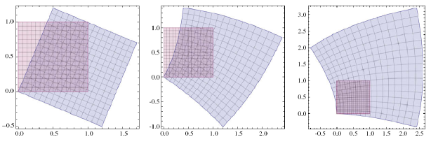
Figure 2: Infinitesimal conformal mappings [83] preserve locally angles and shapes. The corresponding couple stress tensor $\widetilde{m}$ is zero for these deformation modes.

Using the formulas (2.40), it can be easily remarked that $\|\nabla[\operatorname{dev}\operatorname{sym}\nabla u]\|^{2}$, $\|\operatorname{dev}\operatorname{sym}\nabla u\|^{2}$,$\|\operatorname{dev}\operatorname{sym}\nabla(\textrm{curl\,}u)\|^{2}$, $\|\operatorname{sym}\operatorname{Curl\,}(\operatorname{sym}\nabla u)\|^{2}=\frac{1}{4}\,\|\operatorname{sym}\nabla(\textrm{curl\,}u)\|^{2}$ are conformally invariant. Let us note that, using Lemma 2.1, we have

$$\|\operatorname{sym}\operatorname{Curl\,}(\operatorname{sym}\nabla u)\|^{2} =\|\operatorname{sym}\nabla[\operatorname{axl}(\operatorname{skew}\nabla u)]\|^{2}=\frac{1}{4}\,\|\operatorname{sym}\nabla(\textrm{curl\,}u)\|^{2},$$ (2.44)

$$\|\operatorname{skew}[\operatorname{Curl\,}(\operatorname{sym}\nabla u)]\|^{2} =\|\operatorname{skew}\nabla[\operatorname{axl}(\operatorname{skew}\nabla u)]\|^{2}=\frac{1}{4}\,\|\operatorname{skew}\nabla(\textrm{curl\,}u)\|^{2}.$$ (2.45)

Hence $\|\operatorname{sym}\operatorname{Curl\,}(\operatorname{sym}\nabla u)\|^{2}=\frac{1}{4}\,\|\operatorname{sym}\nabla(\textrm{curl\,}u)\|^{2}$ is also conformally invariant (use (2.40)₆), while

$$\|\operatorname{skew}[\operatorname{Curl\,}(\operatorname{sym}\nabla\phi_{c})]\|^{2} =\frac{1}{4}\,\|\operatorname{skew}\nabla(\textrm{curl\,}\phi_{c})\|^{2}=\|\overline{W}\|^{2},$$ (2.46)

and therefore $\|\operatorname{Curl\,}(\operatorname{sym}\nabla u)\|^{2}$ is not conformally invariant, nor is $\|\nabla(\operatorname{axl}(\operatorname{skew}\nabla u))\|^{2}$ conformally invariant. Nor is $\|\nabla\operatorname{tr}(\operatorname{sym}\nabla u)\|^{2}=\|\nabla{\rm div}u\|^{2}$ conformally invariant.

The underlying additional invariance property of the modified couple stress theory is precisely conformal invariance. In the modified couple stress model, these deformations are free of size-effects, while e.g. the Hadjesfandiari and Dargush choice would describe size-effects. In other words, the generated couple stress tensor $\widetilde{m}$ in the modified couple stress model is zero for this inhomogeneous deformation mode, while in the Hadjesfandiari and Dargush choice $\widetilde{m}$ is constant and skew-symmetric.

2.5 The classical indeterminate couple stress model based on
$\|\nabla[\operatorname{axl}(\operatorname{skew}\nabla u)]\|^{2}$ with skew-symmetric nonlocal force-stress

We are now re-deriving the classical equations based on the $\nabla[\operatorname{axl}(\operatorname{skew}\nabla u)]$-formulation of the indeterminate couple stress model. This part does not contain new results, see, e.g., [61] for further details, but is included for setting the stage of our new modelling approach.

Taking free variations $\delta u\in C^{\infty}(\Omega)$ in the energy $W(e,\widetilde{k})=W_{\rm lin}(e)+W_{\rm curv}(\widetilde{k})$, but using the following equivalent curvature energy based on $\widetilde{k}=\nabla[\operatorname{axl}(\operatorname{skew}\nabla u)]=\frac{1}{2}\nabla(\textrm{curl\,}u)$ :

$$W_{\rm curv}(\widetilde{k})= \mu\,L_{c}^{2}\,[\alpha_{1}\,\|\operatorname{dev}\operatorname{sym}\nabla[\operatorname{axl}(\operatorname{skew}\nabla u)]\|^{2}+\alpha_{2}\,\|\operatorname{skew}\nabla[\operatorname{axl}(\operatorname{skew}\nabla u)]\|^{2}]$$ (2.47)

$$= \mu\,L_{c}^{2}\,[\alpha_{1}\,\|\operatorname{dev}\operatorname{sym}\operatorname{Curl\,}(\operatorname{sym}\nabla u)]\|^{2}+\alpha_{2}\,\|\operatorname{skew}\operatorname{Curl\,}(\operatorname{sym}\nabla u)]\|^{2}]\,,$$

we obtain the virtual work principle taking free variations $\delta u\in C^{\infty}(\Omega)$ in the energy (2.47)

$$\frac{\rm d}{\rm dt}\int_{\Omega}W(\nabla u+t\nabla\delta u)dv\Big{|}_{t=0}= \int_{\Omega}\bigg{[}2\mu\,\langle\operatorname{sym}\nabla u,\operatorname{sym}\nabla\delta u\rangle+\lambda\operatorname{tr}(\nabla u)\,\operatorname{tr}(\nabla\delta u)$$

$$+\mu\,L_{c}^{2}\,[2\,\alpha_{1}\,\langle\operatorname{dev}\operatorname{sym}\nabla[\operatorname{axl}(\operatorname{skew}\nabla u)],\operatorname{dev}\operatorname{sym}\nabla[\operatorname{axl}(\operatorname{skew}\nabla\delta u)]\rangle$$ (2.48)

$$+2\,\alpha_{2}\,\langle\operatorname{skew}\nabla[\operatorname{axl}(\operatorname{skew}\nabla u)],\operatorname{skew}\nabla[\operatorname{axl}(\operatorname{skew}\nabla\delta u)]\rangle]+\langle f,\delta u\rangle\bigg{]}dv=0.$$

The classical divergence theorem leads to

$$\int_{\Omega}\langle\textrm{Div\,}(\sigma-\widetilde{\tau})+f,\delta u\rangle\,dv-\int_{\partial\Omega}\langle(\sigma-\widetilde{\tau}).\,n,\delta u\rangle\,dv-\int_{\partial\Omega} \langle\widetilde{{m}}.\,n,\operatorname{axl}(\operatorname{skew}\nabla\delta u)\rangle da=0,$$ (2.49)

for all virtual displacements $\delta u\in C^{\infty}(\Omega)$, where $n$ is the unit outward normal vector at the surface $\partial\Omega$, $\sigma$ is the symmetric local force-stress tensor

$$\sigma=2\,\mu\,\operatorname{sym}\nabla u+\lambda\,\operatorname{tr}(\nabla u)\,{\boldsymbol{\mathbbm{1}}}\!\in{\rm Sym}(3)$$ (2.50)

and $\widetilde{\tau}$ represents the nonlocal force-stress tensor (which here is automatically skew-symmetric)

$$\widetilde{\tau} =\mu\,L_{c}^{2}\,[{\alpha_{1}}\,\operatorname{anti}{\rm Div}(\operatorname{dev}\operatorname{sym}\nabla[\operatorname{axl}(\operatorname{skew}\nabla u)])+{\alpha_{2}}\,\operatorname{anti}{\rm Div}(\operatorname{skew}\nabla[\operatorname{axl}(\operatorname{skew}\nabla u)])$$ (2.51)

$$=\mu\,L_{c}^{2}\,[\frac{\alpha_{1}}{2}\operatorname{anti}{\rm Div}(\operatorname{dev}\operatorname{sym}\nabla(\textrm{curl\,}u))+\frac{\alpha_{2}}{2}\,\operatorname{anti}{\rm Div}(\operatorname{skew}\nabla(\textrm{curl\,}u))]$$

$$=\mu\,L_{c}^{2}\,\operatorname{anti}{\rm Div}\left[\frac{\alpha_{1}}{2}\operatorname{dev}\operatorname{sym}\nabla(\textrm{curl\,}u)+\frac{\alpha_{2}}{2}\,\operatorname{skew}\nabla(\textrm{curl\,}u)\right]=\frac{1}{2}\operatorname{anti}{\rm Div}[\widetilde{{m}}]\in\operatorname{\mathfrak{so}}(3),$$

where

$$\widetilde{{m}} =\mu\,L_{c}^{2}\,[{\alpha_{1}}\operatorname{sym}\nabla(\textrm{curl\,}u)+{\alpha_{2}}\,\operatorname{skew}\nabla(\textrm{curl\,}u)]$$

$$=\mu\,L_{c}^{2}\,[{\alpha_{1}}\operatorname{dev}\operatorname{sym}\nabla(\textrm{curl\,}u)+{\alpha_{2}}\,\operatorname{skew}\nabla(\textrm{curl\,}u)]$$ (2.52)

$$=\mu\,L_{c}^{2}\,[2\,{\alpha_{1}}\operatorname{dev}\operatorname{sym}\nabla[\operatorname{axl}(\operatorname{skew}\nabla u)]+2\,{\alpha_{2}}\,\operatorname{skew}\nabla[\operatorname{axl}(\operatorname{skew}\nabla u)]],$$

is the hyperstress tensor (couple stress tensor) which may or may not be symmetric, depending on the material parameters.

The non-symmetry of force stress is a constitutive assumption. Thus, if the test function $\delta u\in C^{\infty}(\Omega)$ also satisfies $\operatorname{axl}(\operatorname{skew}\nabla\delta u)=0$ on $\Gamma$ (equivalently $\textrm{curl\,}\delta u=0$), then we obtain the equilibrium equation

$$\textrm{Div\,}\bigg{\{} \underbrace{2\,\mu\,\operatorname{sym}\nabla u+\lambda\,\operatorname{tr}(\nabla u)\,{\boldsymbol{\mathbbm{1}}}}_{\text{\rm symmetric local force stress}\ \sigma\in{\rm Sym}(3)}$$

$$-\underbrace{\mu\,L_{c}^{2}\,[\operatorname{anti}\{{\rm Div}(\underbrace{\alpha_{1}\,\operatorname{dev}\operatorname{sym}\nabla[\operatorname{axl}(\operatorname{skew}\nabla u)]+\alpha_{2}\,\operatorname{skew}\nabla[\operatorname{axl}(\operatorname{skew}\nabla u)]}_{\text{\rm hyperstress }\frac{1}{2}\widetilde{m}\in\operatorname{\mathfrak{gl}}(3)})\}]\bigg{\}}}_{\text{\rm completely skew-symmetric nonlocal force stress}\ \widetilde{\tau}\in\operatorname{\mathfrak{so}}(3)}+f=0,$$ (2.53)

or equivalently

$$\textrm{Div\,}\,\widetilde{\sigma}_{\rm total}+f=0,$$ (2.54)

where

$$\widetilde{\sigma}_{\rm total}=\sigma-\widetilde{\tau}\not\in{\rm Sym}(3).$$ (2.55)

The complete consistent boundary conditions for this formulation is presented for the first time in [61, 80] and recapitulated in Figure 4 and Figure 7.

3 The new isotropic gradient elasticity model with symmetric nonlocal force stress and symmetric hyperstresses

As independent constitutive variables for our novel gradient elastic model we choose now

$$\varepsilon=\operatorname{sym}\nabla u,\quad\quad\quad\widehat{k}=\operatorname{Curl\,}(\operatorname{sym}\nabla u)=\operatorname{Curl\,}\varepsilon.$$ (3.1)

We use again the orthogonal Lie-algebra decomposition of $\mathbb{R}^{3\times 3}$

$$\operatorname{Curl\,}(\operatorname{sym}\nabla u) ={\operatorname{dev}\operatorname{sym}(\operatorname{Curl\,}(\operatorname{sym}\nabla u))}+{\operatorname{skew}\operatorname{Curl\,}(\operatorname{sym}\nabla u)}\,.$$ (3.2)

The term $\frac{1}{3}\operatorname{tr}(\operatorname{Curl\,}(\operatorname{sym}\nabla u))\,{\boldsymbol{\mathbbm{1}}}$ is missing since $\operatorname{tr}(\operatorname{Curl\,}(\operatorname{sym}\nabla u))=0$ anyway (already $\operatorname{tr}(\operatorname{Curl\,}S)=0$ for $S\in{\rm Sym}(3)$). The model is derived from the free energy $W(e,\widehat{k})=W_{\rm lin}(e)+W_{\rm curv}(\widehat{k})$, with

$$W_{\rm lin}(\varepsilon) =\,\mu\,\|\operatorname{sym}\nabla u\|^{2}+\frac{\lambda}{2}\,[\operatorname{tr}(\operatorname{sym}\nabla u)]^{2}=\,\mu\,\|\operatorname{dev}\operatorname{sym}\nabla u\|^{2}+\frac{\kappa}{2}\,[\operatorname{tr}(\operatorname{sym}\nabla u)]^{2},$$ (3.3)

$$W_{\rm curv}(\widehat{k}) =\mu\,L_{c}^{2}\,\Big{[}\,\alpha_{1}\,\underbrace{\|\operatorname{dev}\operatorname{sym}\operatorname{Curl\,}(\operatorname{sym}\nabla u)\|^{2}}_{\text{conformally invariant}}+\alpha_{2}\,\underbrace{\|\operatorname{skew}\operatorname{Curl\,}(\operatorname{sym}\nabla u)\|^{2}}_{\text{not conformally invariant}}\Big{]}\,,$$

where $\alpha_{1}$, $\alpha_{2}$ are non-negative constitutive curvature coefficients and $\kappa=\frac{2\mu+3\lambda}{3}$ is the infinitesimal bulk modulus, while $\mu$ is the classical shear modulus.

The hyperstress-tensor (moment stress tensor, couple stress tensor)

$$\widehat{{m}}:=D_{\widehat{k}}W_{\rm curv}(\widehat{k})=\mu\,L_{c}^{2}\,[2\,\alpha_{1}\,\operatorname{dev}\operatorname{sym}\operatorname{Curl\,}(\operatorname{sym}\nabla u)+2\,\alpha_{2}\,\operatorname{skew}\operatorname{Curl\,}(\operatorname{sym}\nabla u)]$$

is symmetric in the conformal case $\alpha_{2}=0$, while the nonlocal force stress tensor is always symmetric, see eq. (3).

Due to isotropy, the curvature energy $W_{\rm curv}(k)$ involves in principle only 2 additional constitutive constants. Taking free variations $\delta u\in C^{\infty}(\Omega)$ in the energy (3.3), we obtain the virtual work principle

$$\frac{\rm d}{\rm dt}\int_{\Omega}W(\nabla u+t\nabla\delta u)dv\Big{|}_{t=0}= \int_{\Omega}\bigg{[}\quad 2\,\mu\,\langle\operatorname{sym}\nabla u,\operatorname{sym}\nabla\delta u\rangle+\lambda\operatorname{tr}(\nabla u)\,\operatorname{tr}(\nabla\delta u)$$

$$\qquad+\mu\,L_{c}^{2}\,[2\,\alpha_{1}\,\langle\operatorname{dev}\operatorname{sym}\operatorname{Curl\,}(\operatorname{sym}\nabla u),\operatorname{dev}\operatorname{sym}\operatorname{Curl\,}(\operatorname{sym}\nabla\delta u)\rangle$$ (3.4)

$$\qquad+2\,\alpha_{2}\,\langle\operatorname{skew}\operatorname{Curl\,}(\operatorname{sym}\nabla u),\operatorname{skew}\operatorname{Curl\,}(\operatorname{sym}\nabla\delta u)\rangle]+\langle f,\delta u\rangle\bigg{]}dv=0,$$

where $f$ is the body force per unit volume. We have the formulas

$${\rm div}(\varphi_{i}\,Q_{i}) =\langle Q_{i},\nabla\,\varphi_{i}\rangle+\varphi_{i}\,{\rm div}\,Q_{i}\,\qquad\qquad\text{not summed},$$ (3.5)

$${\rm div}\,(R_{i}\times S_{i}) =\langle S_{i},\textrm{curl\,}\,R_{i}\rangle-\langle R_{i},\textrm{curl\,}\,S_{i}\rangle\,\quad\ \ \text{not summed},$$

for all $C^{1}$-functions $\varphi_{i}:\Omega\rightarrow\mathbb{R}$ and $Q_{i},P_{i},S_{i}:\Omega\rightarrow\mathbb{R}^{3}$, where $\varphi_{i}$ are the components of the vector $\varphi$ and $Q_{i},P_{i},S_{i}$ are the rows of the matrix $Q$, $P$ and $S$, respectively, where $\times$ denotes the vector product. If we take in (3.5) $R_{i}=[\operatorname{dev}\operatorname{sym}\operatorname{Curl\,}(\operatorname{sym}\nabla u)]_{i},S_{i}=(\operatorname{sym}\nabla\delta u)_{i}\,,$ we get

$$\sum\limits_{i=1}^{3}{\rm div}\,([\operatorname{dev}\operatorname{sym}\operatorname{Curl\,}(\operatorname{sym}\nabla u)]_{i}\times(\operatorname{sym}\nabla\delta u)_{i})= \sum\limits_{i=1}^{3}\langle(\operatorname{sym}\nabla\delta u)_{i},\textrm{curl\,}\,[\operatorname{dev}\operatorname{sym}\operatorname{Curl\,}(\operatorname{sym}\nabla u)]_{i}\rangle$$ (3.6)

$$-\sum\limits_{i=1}^{3}\langle[\operatorname{dev}\operatorname{sym}\operatorname{Curl\,}(\operatorname{sym}\nabla u)]_{i},\textrm{curl\,}\,(\operatorname{sym}\nabla\delta u)_{i}\rangle\,.$$

Hence, we obtain

$$\sum\limits_{i=1}^{3}{\rm div}\,([\operatorname{dev}\operatorname{sym}\operatorname{Curl\,}(\operatorname{sym}\nabla u)]_{i}\times(\operatorname{sym}\nabla\delta u)_{i})= \langle(\operatorname{sym}\nabla\delta u),\operatorname{Curl\,}\,[\operatorname{dev}\operatorname{sym}\operatorname{Curl\,}(\operatorname{sym}\nabla u)]\rangle$$ (3.7)

$$-\langle[\operatorname{dev}\operatorname{sym}\operatorname{Curl\,}(\operatorname{sym}\nabla u)],\operatorname{Curl\,}(\operatorname{sym}\nabla\delta u)\rangle\,.$$

Doing a similar calculus, but choosing $R_{i}=[\operatorname{skew}\operatorname{Curl\,}(\operatorname{sym}\nabla u)]_{i},S_{i}=(\operatorname{sym}\nabla\delta u)_{i},$ we obtain

$$\sum\limits_{i=1}^{3}{\rm div}\,([\operatorname{skew}\operatorname{Curl\,}(\operatorname{sym}\nabla u)]_{i}\times(\operatorname{sym}\nabla\delta u)_{i})= \langle(\operatorname{sym}\nabla\delta u),\operatorname{Curl\,}\,[\operatorname{skew}\operatorname{Curl\,}(\operatorname{sym}\nabla u)]\rangle$$ (3.8)

$$-\langle[\operatorname{skew}\operatorname{Curl\,}(\operatorname{sym}\nabla u)],\operatorname{Curl\,}(\operatorname{sym}\nabla\delta u)\rangle\,.$$

The above formulas lead, for all variations $\delta u\in C^{\infty}(\Omega)$, to

$$\int_{\Omega}\bigg{[} \alpha_{1}\,\langle\operatorname{dev}\operatorname{sym}\operatorname{Curl\,}(\operatorname{sym}\nabla u),\operatorname{Curl\,}(\operatorname{sym}\nabla\delta u)\rangle+\alpha_{2}\,\langle\operatorname{skew}\operatorname{Curl\,}(\operatorname{sym}\nabla u),\operatorname{Curl\,}(\operatorname{sym}\nabla\delta u)\rangle\bigg{]}dv$$

$$=\int_{\Omega}\bigg{[}\alpha_{1}\,\langle\operatorname{sym}\operatorname{Curl\,}\,[\operatorname{dev}\operatorname{sym}\operatorname{Curl\,}(\operatorname{sym}\nabla u)],\nabla\delta u,\rangle+\alpha_{2}\,\langle\operatorname{sym}\operatorname{Curl\,}\,[\operatorname{skew}\operatorname{Curl\,}(\operatorname{sym}\nabla u)],\nabla\delta u,\rangle$$ (3.9)

$$\quad-\sum\limits_{i=1}^{3}{\rm div}\,\bigg{[}\alpha_{1}\,([\operatorname{dev}\operatorname{sym}\operatorname{Curl\,}(\operatorname{sym}\nabla u)]_{i}\times(\operatorname{sym}\nabla\delta u)_{i})+\alpha_{2}([\operatorname{skew}\operatorname{Curl\,}(\operatorname{sym}\nabla u)]_{i}\times(\operatorname{sym}\nabla\delta u)_{i})\bigg{]}dv$$

$$=\int_{\Omega}\bigg{[}\alpha_{1}\,\langle\operatorname{sym}\operatorname{Curl\,}\,[\operatorname{dev}\operatorname{sym}\operatorname{Curl\,}(\operatorname{sym}\nabla u)],\nabla\delta u\rangle+\alpha_{2}\,\langle\operatorname{sym}\operatorname{Curl\,}\,[\operatorname{skew}\operatorname{Curl\,}(\operatorname{sym}\nabla u)],\nabla\delta u\rangle$$

$$\quad-\sum\limits_{i=1}^{3}{\rm div}\,\bigg{[}\alpha_{1}\,([\operatorname{dev}\operatorname{sym}\operatorname{Curl\,}(\operatorname{sym}\nabla u)]_{i}\times(\operatorname{sym}\nabla\delta u)_{i})+\alpha_{2}([\operatorname{skew}\operatorname{Curl\,}(\operatorname{sym}\nabla u)]_{i}\times(\operatorname{sym}\nabla\delta u)_{i})\bigg{]}dv\,.$$

Therefore, using the divergence theorem and a special format of the partial integration which is suggested by the matrix $\operatorname{Curl\,}$-operator, it follows that

$$\int_{\Omega}\bigg{[} \alpha_{1}\,\langle\operatorname{dev}\operatorname{sym}\operatorname{Curl\,}(\operatorname{sym}\nabla u),\operatorname{Curl\,}(\operatorname{sym}\nabla\delta u)\rangle+\alpha_{2}\,\langle\operatorname{skew}\operatorname{Curl\,}(\operatorname{sym}\nabla u),\operatorname{Curl\,}(\operatorname{sym}\nabla\delta u)\rangle\bigg{]}dv$$ (3.10)

$$=\int_{\Omega}\bigg{[}\alpha_{1}\,\langle\operatorname{sym}\operatorname{Curl\,}\,[\operatorname{dev}\operatorname{sym}\operatorname{Curl\,}(\operatorname{sym}\nabla u)],\nabla\delta u\rangle+\alpha_{2}\,\langle\operatorname{sym}\operatorname{Curl\,}\,[\operatorname{skew}\operatorname{Curl\,}(\operatorname{sym}\nabla u)],\nabla\delta u\rangle\bigg{]}dv$$

$$\quad-\int_{\partial\Omega}\bigg{[}\sum\limits_{i=1}^{3}\langle\alpha_{1}\,([\operatorname{dev}\operatorname{sym}\operatorname{Curl\,}(\operatorname{sym}\nabla u)]_{i}\times(\operatorname{sym}\nabla\delta u)_{i})+\alpha_{2}([\operatorname{skew}\operatorname{Curl\,}(\operatorname{sym}\nabla u)]_{i}\times(\operatorname{sym}\nabla\delta u)_{i}),n\rangle da$$

$$=-\int_{\Omega}\bigg{[}\alpha_{1}\,\langle\textrm{Div\,}\{\operatorname{sym}\operatorname{Curl\,}\,[\operatorname{dev}\operatorname{sym}\operatorname{Curl\,}(\operatorname{sym}\nabla u)]+\alpha_{2}\,\langle\operatorname{sym}\operatorname{Curl\,}\,[\operatorname{skew}\operatorname{Curl\,}(\operatorname{sym}\nabla u)]\},\delta u\rangle\bigg{]}dv$$

$$\qquad+\int_{\partial\Omega}\langle\bigg{[}\alpha_{1}\,\operatorname{sym}\operatorname{Curl\,}\,[\operatorname{dev}\operatorname{sym}\operatorname{Curl\,}(\operatorname{sym}\nabla u)]+\alpha_{2}\,\operatorname{sym}\operatorname{Curl\,}\,[\operatorname{skew}\operatorname{Curl\,}(\operatorname{sym}\nabla u)\bigg{]}.\,n,\delta u\rangle da$$

$$\qquad-\int_{\partial\Omega}\bigg{[}\sum\limits_{i=1}^{3}\langle\alpha_{1}\,[\operatorname{dev}\operatorname{sym}\operatorname{Curl\,}(\operatorname{sym}\nabla u)]_{i}+\alpha_{2}[\operatorname{skew}\operatorname{Curl\,}(\operatorname{sym}\nabla u)]_{i},(\operatorname{sym}\nabla\delta u)_{i}\times n\rangle da,$$

where $n$ is the unit outward normal vector at the surface $\partial\Omega$. Hence, the relation (3) leads to

$$\int_{\Omega}\textrm{Div\,}\bigg{\{}2 \,\mu\,\operatorname{sym}\nabla u+\lambda\,\operatorname{tr}(\nabla u)\,{\boldsymbol{\mathbbm{1}}}$$ (3.11)

$$+\mu\,L_{c}^{2}\,[2\,\alpha_{1}\operatorname{sym}\operatorname{Curl\,}\,[\operatorname{dev}\operatorname{sym}\operatorname{Curl\,}(\operatorname{sym}\nabla u)]+2\,\alpha_{2}\,\operatorname{sym}\operatorname{Curl\,}\,[\operatorname{skew}\operatorname{Curl\,}(\operatorname{sym}\nabla u)]]\bigg{\}}+f,\delta u\rangle\,dv$$

$$-\int_{\partial\Omega} \bigg{[}\langle\bigg{[}2\mu\,\langle\operatorname{sym}\nabla u+\lambda\,\operatorname{tr}(\nabla u)\,{\boldsymbol{\mathbbm{1}}}\bigg{]}.\,n,\delta u\rangle da$$

$$-\int_{\partial\Omega} \langle 2\,\mu\,L_{c}^{2}\,\bigg{[}\alpha_{1}\,\operatorname{sym}\operatorname{Curl\,}\,[\operatorname{dev}\operatorname{sym}\operatorname{Curl\,}(\operatorname{sym}\nabla u)]+\alpha_{2}\,\operatorname{sym}\operatorname{Curl\,}\,[\operatorname{skew}\operatorname{Curl\,}(\operatorname{sym}\nabla u)]\bigg{]}.\,n,\delta u\rangle da$$

$$\qquad+\int_{\partial\Omega} \bigg{[}\sum\limits_{i=1}^{3}2\,\mu\,L_{c}^{2}\,\langle\alpha_{1}\,[\operatorname{dev}\operatorname{sym}\operatorname{Curl\,}(\operatorname{sym}\nabla u)]_{i}+\alpha_{2}[\operatorname{skew}\operatorname{Curl\,}(\operatorname{sym}\nabla u)]_{i},(\operatorname{sym}\nabla\delta u)_{i}\times n\rangle da=0,$$

for all variations $\delta u\in C^{\infty}(\Omega)$.

We can write the above variational formulation, for all variations $\delta u\in C^{\infty}(\Omega)$, in the following form

$$\int_{\Omega}\langle\textrm{Div\,}(\sigma+\widehat{\tau})+f,\delta u\rangle\,dv-\int_{\partial\Omega}\langle(\sigma+\widehat{\tau}).\,n,\delta u\rangle da-\int_{\partial\Omega}\sum\limits_{i=1}^{3}\langle\widehat{{m}}_{i}\times n,(\operatorname{sym}\nabla\delta u)_{i}\rangle da=0,$$ (3.12)

where

$$\sigma =2\,\mu\,\operatorname{sym}\nabla u+\lambda\,\operatorname{tr}(\nabla u)\,{\boldsymbol{\mathbbm{1}}}\in{\rm Sym}(3),\qquad\qquad\qquad\qquad\qquad\qquad\quad\ \text{(local force-stress)}\vspace{1.5mm}$$

$$\widehat{\tau} =\mu\,L_{c}^{2}\,\operatorname{sym}\{2\,\alpha_{1}\operatorname{Curl\,}\,[\operatorname{dev}\operatorname{sym}\operatorname{Curl\,}(\operatorname{sym}\nabla u)]+2\,\alpha_{2}\,\operatorname{Curl\,}\,[\operatorname{skew}\operatorname{Curl\,}(\operatorname{sym}\nabla u)]\}$$ (3.13)

$$=\operatorname{sym}\operatorname{Curl\,}(\widehat{{m}})\in{\rm Sym}(3),\qquad\qquad\qquad\qquad\qquad\qquad\qquad\qquad\qquad\text{(non-local force stress)}\vspace{1.5mm}$$

$$\widehat{{m}} =\mu\,L_{c}^{2}\,\{2\,\alpha_{1}\operatorname{dev}\operatorname{sym}[\operatorname{Curl\,}(\operatorname{sym}\nabla u)]+2\,\alpha_{2}\,\operatorname{skew}[\operatorname{Curl\,}(\operatorname{sym}\nabla u)]\}\in\operatorname{\mathfrak{gl}}(3)\qquad(\in{\rm Sym}(3)\ \ \text{for}\ \ \alpha_{2}=0).$$

We call $\sigma$ the local force stress tensor, $\widehat{\tau}$ the non-local force stress tensor and $\widehat{{m}}=D_{\widehat{k}}W_{\rm curv}(\widehat{k})$ the hyperstress tensor (couple stress tensor).

Thus, if the test function $\delta u\in C^{\infty}(\Omega)$ also satisfies $(\operatorname{sym}\nabla\delta u)_{i}\times n=0$ (or equivalently $(\operatorname{sym}\nabla\delta u).\tau=0$ for all tangential vectors $\tau$ at $\Gamma$), then we obtain the equilibrium equation

$$\textrm{Div\,}\{\!\!\!\!\!\! \underbrace{2\,\mu\,\operatorname{sym}\nabla u+\lambda\,\operatorname{tr}(\nabla u)\,{\boldsymbol{\mathbbm{1}}}}_{\text{symmetric local force stress}\ \sigma\,\in\,{\rm Sym}(3)}$$

$$\quad+\underbrace{\mu\,L_{c}^{2}\,\operatorname{sym}\operatorname{Curl\,}\,[\underbrace{2\,\alpha_{1}\operatorname{dev}\operatorname{sym}\operatorname{Curl\,}(\operatorname{sym}\nabla u)+2\,\alpha_{2}\,\operatorname{skew}\operatorname{Curl\,}(\operatorname{sym}\nabla u)}_{\text{hyperstress}\ \widehat{{m}}\in\operatorname{\mathfrak{gl}}(3)}]}_{\text{symmetric nonlocal force stress}\ \widehat{\tau}\,\in\,{\rm Sym}(3)}\}+f=0.$$ (3.14)

The first impulse is to prescribe on $\Gamma\subseteq\partial\Omega$ the following geometric boundary conditions

$$u =\widehat{u}^{0}\qquad\ \qquad\qquad\quad\ \qquad\qquad\quad\qquad\qquad\qquad\quad\text{on}\qquad\Gamma,$$ (3.15)

$$({\boldsymbol{\mathbbm{1}}}-n\otimes n)\,(\operatorname{sym}\nabla u)_{i}\times n =({\boldsymbol{\mathbbm{1}}}-n\otimes n)\,(\operatorname{sym}\nabla\widehat{u}^{0})_{i}\times n,\quad i=1,2,3\qquad\quad\,\text{on}\qquad\Gamma,$$

where $\widehat{u}^{0}:\mathbb{R}^{3}\rightarrow\mathbb{R}^{3}$ is a prescribed function (i.e. 3+2+2+2=9 boundary conditions), with $\widehat{u}^{0}\in H^{2,2}(\Omega)$, and the following traction boundary conditions on $\partial\Omega\setminus\overline{\Gamma}$

$$(\sigma+\widehat{\tau}).n =\widehat{g},\ \ \qquad\qquad\qquad\qquad\quad\quad\qquad\quad\qquad\text{on}\qquad\partial\Omega\setminus\overline{\Gamma},$$ (3.16)

$$({\boldsymbol{\mathbbm{1}}}-n\otimes n)\,\widehat{m}_{i}\times n =({\boldsymbol{\mathbbm{1}}}-n\otimes n)\,\widehat{g}_{i},\quad i=1,2,3\ \qquad\quad\quad\ \ \text{on}\qquad\partial\Omega\setminus\overline{\Gamma},$$

where $\widehat{g},\widehat{g}_{i}:\mathbb{R}^{3}\rightarrow\mathbb{R}^{3}$ are prescribed functions (i.e. 3+2+2+2=9 boundary conditions).

However, we need to separate normal and tangential derivatives of the test function $\delta u$ in (3.12) which is standard in general strain gradient elasticity, since tangential derivatives of $\delta u$ are not independent of $\delta u$. Let us define the matrix

$$\widehat{M}:=\left(\begin{array}[]{c}\widehat{m}_{1}\times n\_\_\_\_\\ \widehat{m}_{2}\times n\_\_\_\_\\ \widehat{m}_{3}\times n\_\_\_\_\\ \end{array}\right),\qquad\text{where}\qquad\widehat{m}:=\left(\begin{array}[]{c}\widehat{m}_{1}\_\_\_\_\\ \widehat{m}_{2}\_\_\_\_\\ \widehat{m}_{3}\_\_\_\_\\ \end{array}\right).$$ (3.23)

With the help of this matrix $\widehat{M}$, we may write

$$\sum\limits_{i=1}^{3}\langle\widehat{{m}}_{i}\times n,(\operatorname{sym}\nabla\delta u)_{i}\rangle=\langle\widehat{M},\operatorname{sym}\nabla\delta u\rangle=\langle\operatorname{sym}\widehat{M},\nabla\delta u\rangle.$$ (3.24)

At this point, it must be considered that the tangential trace of the gradient of virtual displacement can be integrated by parts once again and that the surface divergence theorem can be applied to this tangential part of $\nabla\delta{u}$. Before doing so, one needs to introduce (see also [24, 99, 22] for details) two second order tensors $T$ and $Q$ which are the two projectors on the tangent plane and on the normal to the considered surface, respectively. As it is well known from differential geometry, such projectors actually allow to split a given vector or tensor field in one part projected on the plane tangent to the considered surface and one projected on the normal to such surface (see e.g. [24]). Let $\left\{\tau^{1},\tau^{2}\right\}$ be an orthonormal local basis of the tangent plane to the considered surface at point $p$ and let ${n}$ be the unit normal vector at the same point. We can introduce the quoted projectors as

$$T =\tau^{1}\otimes\tau^{1}+\tau^{2}\otimes\tau^{2}={\boldsymbol{\mathbbm{1}}}-{n}\otimes{n}\quad(T_{ij}=\delta_{ij}-n_{i}n_{j}),\qquad{Q}={n}\otimes{n}\qquad(Q_{ij}=n_{i}n_{j}).$$ (3.25)

In our abbreviations, the surface divergence theorem means [40, p. 58, ex. 7]

$$\int_{\partial S}\langle T.\,v,{\nu}\rangle da=\int_{\partial S}\langle v,T.\,{\nu}\rangle da=\int_{\partial S}\langle v,{\nu}\rangle ds\,,$$ (3.26)

for any field $v\in\mathbb{R}^{3}$ and $\nu=\tau\times n$. Regarding the boundary conditions, similar as in [71], we obtain

$$\begin{array}[]{ll}\displaystyle\sum\limits_{i=1}^{3}&\langle\widehat{{m}}_{i}\times n,(\operatorname{sym}\nabla\delta u)_{i}\rangle=\langle\operatorname{sym}\widehat{M},\nabla\delta u\,{\boldsymbol{\mathbbm{1}}}\rangle=\langle\operatorname{sym}\widehat{M},\nabla\delta u\,(T+Q)\rangle\vspace*{-3mm}\\ &=\langle(\operatorname{sym}\widehat{M}),(\nabla\delta u)\,T\rangle+\langle(\operatorname{sym}\widehat{M}),(\nabla\delta u)\,Q\rangle=\langle(\operatorname{sym}\widehat{M})\,T,\nabla\delta u\rangle+\langle(\operatorname{sym}\widehat{M}),(\nabla\delta u)\,Q\rangle\\ &=\langle(\operatorname{sym}\widehat{M})\,T\,T,\nabla\delta u\rangle+\langle(\operatorname{sym}\widehat{M}),(\nabla\delta u)\,Q\rangle=\langle\,T,T(\operatorname{sym}\widehat{M})\nabla\delta u\rangle+\langle(\operatorname{sym}\widehat{M}),(\nabla\delta u)\,Q\rangle\\ &=\langle\,T,T(\operatorname{sym}\widehat{M})\nabla\delta u\rangle+\langle(\operatorname{sym}\widehat{M}),(\nabla\delta u)\,n\otimes n\rangle.\end{array}$$

The last term on the right hand side may be rewritten in the form

$$\begin{array}[]{ll}\langle(\operatorname{sym}\widehat{M}),(\nabla\delta u)\,Q\rangle&=\displaystyle\frac{1}{2}\langle\widehat{M},(\nabla\delta u)\,Q+Q(\nabla\delta u)^{T}\rangle=\displaystyle\frac{1}{2}\langle\widehat{M}\,Q,\nabla\delta u\rangle+\frac{1}{2}\langle\widehat{M},Q(\nabla\delta u)^{T}\rangle\vspace{2mm}\\ &=\displaystyle\frac{1}{2}\langle\widehat{M}\,n\otimes n,\nabla\delta u\rangle+\frac{1}{2}\langle\widehat{M},n\otimes n(\nabla\delta u)^{T}\rangle.\end{array}$$ (3.27)

Thus, we deduce

$$\begin{array}[]{ll}\displaystyle\sum\limits_{i=1}^{3}&\langle\widehat{{m}}_{i}\times n,(\operatorname{sym}\nabla\delta u)_{i}\rangle=\langle\,T,T(\operatorname{sym}\widehat{M})\nabla\delta u\rangle+\displaystyle\langle(\operatorname{sym}\widehat{M}),(\nabla\delta u)\,Q\rangle\vspace*{-3mm}\\ &=\langle\,T,T(\operatorname{sym}\widehat{M})\nabla\delta u\rangle+\displaystyle\langle(\operatorname{sym}\widehat{M}),(\nabla\delta u)\,n\otimes n\rangle=\langle\,T,T(\operatorname{sym}\widehat{M})\nabla\delta u\rangle+\displaystyle\langle\{n\otimes[(\nabla\delta u).n]\}(\operatorname{sym}\widehat{M}),{\boldsymbol{\mathbbm{1}}}\rangle\\ &=\langle\,T,T(\operatorname{sym}\widehat{M})\nabla\delta u\rangle+\displaystyle\langle n\otimes\{(\operatorname{sym}\widehat{M})(\nabla\delta u).n\},{\boldsymbol{\mathbbm{1}}}\rangle=\langle\,T,T(\operatorname{sym}\widehat{M})\nabla\delta u\rangle+\displaystyle\langle n,(\operatorname{sym}\widehat{M})(\nabla\delta u).n\rangle\\ &=\langle\,T,T(\operatorname{sym}\widehat{M})\nabla\delta u\rangle+\displaystyle\langle(\operatorname{sym}\widehat{M}).n,(\nabla\delta u).n\rangle=\langle\,T,T(\operatorname{sym}\widehat{M})\nabla\delta u\rangle+\displaystyle\langle(\operatorname{sym}\widehat{M}).n,\frac{\partial\delta u}{\partial n}\rangle\,.\end{array}$$

We can therefore recognize in the last term of this formula that the normal derivative

$$\frac{\partial}{\partial n}\,\delta u=(\nabla\delta u).n=(\delta u_{i,h}n_{h})_{i}$$ (3.28)

of the test function field $\delta u$ (the virtual displacement) appears. As for the other term, it can be manipulated suitably integrating by parts and then using the surface divergence theorem (3.26), so that we can finally write the last summand from (3.12) in the form

$$\int_{\partial\Omega}\sum\limits_{i=1}^{3}\langle\widehat{{m}}_{i}\times n,(\operatorname{sym}\nabla\delta u)_{i}\rangle da= \int_{\Gamma}\sum\limits_{i=1}^{3}\langle\widehat{{m}}_{i}\times n,(\operatorname{sym}\nabla\delta u)_{i}\rangle da+\int_{\partial\Omega\setminus\overline{\Gamma}}\sum\limits_{i=1}^{3}\langle\widehat{{m}}_{i}\times n,(\operatorname{sym}\nabla\delta u)_{i}\rangle da.$$ (3.29)

We deduce by gathering the results in (3.27)-(3.29) that the last integral on the right hand side is given by

$$\int_{\partial\Omega\setminus\overline{\Gamma}}\sum\limits_{i=1}^{3}\langle\widehat{{m}}_{i}\times n,(\operatorname{sym}\nabla\delta u)_{i}\rangle da=\int_{\partial\Omega\setminus\overline{\Gamma}}\langle\,T,T(\operatorname{sym}\widehat{M})\nabla\delta u\rangle da+\int_{\partial\Omega\setminus\overline{\Gamma}}\displaystyle\langle(\operatorname{sym}\widehat{M}).n,(\nabla\delta u).n\rangle da.$$ (3.30)

Since

$$\{\nabla[\underbrace{T(\operatorname{sym}\widehat{M})\delta u}_{\in\mathbb{R}^{3}}]\}_{ik} =\{T(\operatorname{sym}\widehat{M})).\delta u\}_{i,k}=\{\big{(}T(\operatorname{sym}\widehat{M})\big{)}_{ij}(\delta u)_{j}\}_{,k}$$

$$=\big{(}T(\operatorname{sym}\widehat{M})\big{)}_{ij,k}(\delta u)_{j}+\big{(}T(\operatorname{sym}\widehat{M})\big{)}_{ij}(\delta u)_{j,k}$$ (3.31)

$$=\big{(}T(\operatorname{sym}\widehat{M})\big{)}_{ij,k}(\delta u)_{j}+\big{(}T(\operatorname{sym}\widehat{M})\big{)}_{ij}(\nabla\delta u)_{jk}$$

$$=\big{(}T(\operatorname{sym}\widehat{M})\big{)}_{ij,k}(\delta u)_{j}+\{T(\operatorname{sym}\widehat{M})\,\nabla\delta u\}_{ik},$$

we obtain

$$\int_{\partial\Omega\setminus\overline{\Gamma}}\sum\limits_{i=1}^{3}\langle\widehat{{m}}_{i}\times n,(\operatorname{sym}\nabla\delta u)_{i}\rangle da= \int_{\partial\Omega\setminus\overline{\Gamma}}\langle\,\underbrace{T,\nabla[T(\operatorname{sym}\widehat{M}).\,\delta u]}_{\text{surface divergence is to be used}}\rangle da-\int_{\partial\Omega\setminus\overline{\Gamma}}T_{ik}\big{(}T(\operatorname{sym}\widehat{M})\big{)}_{ij,k}(\delta u)_{j}da$$ (3.32)

$$+\int_{\partial\Omega\setminus\overline{\Gamma}}\displaystyle\langle(\operatorname{sym}\widehat{M}).n,(\nabla\delta u).n\rangle da.$$

In order to write in a compact form the above relation, let us remark that

$$\big{(}T(\operatorname{sym}\widehat{M})\big{)}_{ij} =T_{il}(\operatorname{sym}\widehat{M})_{lj}=T_{il}(\operatorname{sym}\widehat{M})_{jl}=T_{li}(\operatorname{sym}\widehat{M})_{jl}=(\operatorname{sym}\widehat{M})_{jl}T_{li}=\{(\operatorname{sym}\widehat{M})\,T\}_{ji},$$

and further that

$$\big{(}T(\operatorname{sym}\widehat{M})\big{)}_{ij,k}\,T_{ik} =\{(\operatorname{sym}\widehat{M})\,T\}_{ji,k}\,T_{ik}=\big{(}\nabla[(\operatorname{sym}\widehat{M})\,T]:T\big{)}_{j}.$$ (3.33)

We obtain

$$T_{ik}\big{(}T(\operatorname{sym}\widehat{M})\big{)}_{ij,k}(\delta u)_{j}=\big{(}\nabla[(\operatorname{sym}\widehat{M})\,T]:T\big{)}_{j}(\delta u)_{j}=\langle\nabla[(\operatorname{sym}\widehat{M})\,T]:T,\delta u\rangle.$$ (3.34)

We deduce by gathering the results in (3.27)-(3.29) that the last integral on the right hand side is given by

$$\int_{\partial\Omega\setminus\overline{\Gamma}}\sum\limits_{i=1}^{3}\langle\widehat{{m}}_{i}\times n,(\operatorname{sym}\nabla\delta u)_{i}\rangle da$$

$$=\int_{\partial\Omega\setminus\overline{\Gamma}}\langle\,\underbrace{T,\nabla[T(\operatorname{sym}\widehat{M}).\,\delta u]}_{\text{surface divergence is to be used}}\rangle da-\int_{\partial\Omega\setminus\overline{\Gamma}}\langle\nabla[(\operatorname{sym}\widehat{M})\,T]:T,\delta u\rangle da+\,\int_{\partial\Omega\setminus\overline{\Gamma}}\langle(\operatorname{sym}\widehat{M}).n,(\nabla\delta u).n\rangle da$$

$$=-\int_{\partial\Omega\setminus\overline{\Gamma}}\langle\nabla[(\operatorname{sym}\widehat{M})\,T]:T,\delta u\rangle da+\,\int_{\partial\Omega\setminus\overline{\Gamma}}\langle(\operatorname{sym}\widehat{M}).n,(\nabla\delta u).n\rangle da+\int_{\partial(\partial\Omega\setminus\overline{\Gamma})}\langle[(\operatorname{sym}\widehat{M})]^{-}.\nu^{-},\delta u\rangle ds.$$

In the above computation $\nabla[(\operatorname{sym}\widehat{M})\,T]$ is not a matrix, rather a third order tensor and $\nabla[(\operatorname{sym}\widehat{M})\,T]:T\in\mathbb{R}^{3}$ is a contraction operation, i.e.

$$\{\nabla[(\operatorname{sym}\widehat{M})\,T]:T\}_{i}=\{(\operatorname{anti}[(\operatorname{sym}\widehat{M})\,T\}_{ij,k}.T_{jk}.$$

Similar, we handle the corresponding integral on $\partial\Gamma$ from (3.29)

$$\int_{\Gamma}\sum\limits_{i=1}^{3} \langle\widehat{{m}}_{i}\times n,(\operatorname{sym}\nabla\delta u)_{i}\rangle da$$ (3.35)

$$=-\int_{\Gamma}\langle\nabla[(\operatorname{sym}\widehat{M})\,T]:T,\delta u\rangle da+\,\int_{\Gamma}\langle(\operatorname{sym}\widehat{M}).n,(\nabla\delta u).n\rangle da+\int_{\partial\Gamma}\langle[(\operatorname{sym}\widehat{M})]^{+}.\nu^{+},\delta u\rangle ds.$$

Therefore, the variational formulation (3.12) can be rewritten as

$$\int_{\Omega}\langle\textrm{Div\,}(\sigma+\widehat{\tau})+f,\delta u\rangle\,dv -\int_{\partial\Omega}\underbrace{\langle\underbrace{(\sigma+\widehat{\tau}).\,n-\nabla[(\operatorname{sym}\widehat{M})\,T]:T}_{\begin{array}[]{c}\footnotesize{\delta u}-\text{\footnotesize{surface contact forces depending}}\vspace{-0.5mm}\\ \text{\footnotesize{on the curvature of the boundary}}\end{array}},\delta u\rangle}_{\delta u-\text{independent first order variation}}da$$ (3.38)

$$-\,\int_{\partial\Omega}\underbrace{\langle\underbrace{(\operatorname{sym}\widehat{M}).n}_{\text{double force}},(\nabla\delta u).n\rangle}_{\begin{array}[]{c}\footnotesize{\delta u}-\text{\footnotesize{independent second order}}\vspace{-0.5mm}\\ \text{\footnotesize{normal variation of the gradient}}\end{array}}da-\int_{\partial\Gamma}\underbrace{\langle([\operatorname{sym}\widehat{M}]^{+}-[\operatorname{sym}\widehat{M}]^{-}).\,\nu,\delta u\rangle}_{\text{``edge line force"}}ds=0,$$ (3.41)

for all variations $\delta u\in C^{\infty}(\Omega)$, where we have used that for the regular surface $\partial\Omega$ it holds $\nu^{+}=-\nu^{-}=\nu$. Moreover, we also obtain

$$\widehat{M}.n=\left[\left(\begin{array}[]{c}\widehat{m}_{1}\times n\\ \widehat{m}_{2}\times n\\ \widehat{m}_{3}\times n\\ \end{array}\right).n\right]=\left[\left(\begin{array}[]{c}\langle\widehat{m}_{1}\times n,n\rangle\\ \langle\widehat{m}_{2}\times n,n\rangle\\ \langle\widehat{m}_{3}\times n,n\rangle\\ \end{array}\right).n\right]=0.$$ (3.48)

Hence

$$(\operatorname{sym}\widehat{M}).n=\frac{1}{2}\widehat{M}^{T}.n.$$ (3.49)

On the other hand, we deduce

$$\widehat{M}^{T}.n =T\,\widehat{M}^{T}.n+Q\,\widehat{M}^{T}.n=({\boldsymbol{\mathbbm{1}}}-n\otimes n)\,\widehat{M}^{T}.n+n\otimes n\,\widehat{M}^{T}.n$$

$$=({\boldsymbol{\mathbbm{1}}}-n\otimes n)\,\widehat{M}^{T}.n+[n\otimes n\,\widehat{M}^{T}].n=({\boldsymbol{\mathbbm{1}}}-n\otimes n)\,\widehat{M}^{T}.n+n\otimes[\widehat{M}.\,n].n$$

$$=({\boldsymbol{\mathbbm{1}}}-n\otimes n)\,\widehat{M}^{T}.n+n\otimes\left[\left(\begin{array}[]{c}\widehat{m}_{1}\times n\\ \widehat{m}_{2}\times n\\ \widehat{m}_{3}\times n\\ \end{array}\right).n\right].n=({\boldsymbol{\mathbbm{1}}}-n\otimes n)\,\widehat{M}^{T}.n+n\otimes\left[\left(\begin{array}[]{c}\langle\widehat{m}_{1}\times n,n\rangle\\ \langle\widehat{m}_{2}\times n,n\rangle\\ \langle\widehat{m}_{3}\times n,n\rangle\\ \end{array}\right)\right].n$$ (3.56)

$$=({\boldsymbol{\mathbbm{1}}}-n\otimes n)\,\widehat{M}^{T}.n+[n\otimes 0].n=({\boldsymbol{\mathbbm{1}}}-n\otimes n)\,\widehat{M}^{T}.n\,.$$

In view of (3.49), we see

$$(\operatorname{sym}\widehat{M}).n=({\boldsymbol{\mathbbm{1}}}-n\otimes n)\,(\operatorname{sym}\widehat{M}).n\,.$$ (3.57)

Therefore, finally we get from (3.12)

$$\int_{\Omega}\langle\textrm{Div\,}(\sigma+ \widehat{\tau})+f,\delta u\rangle\,dv-\int_{\partial\Omega}\underbrace{\langle(\sigma+\widehat{\tau}).\,n-\nabla[(\operatorname{sym}\widehat{M})\,T]:T,\delta u\rangle}_{\delta u-\text{independent first order variation}}da$$ (3.58)

$$-\,\int_{\partial\Omega}\underbrace{\langle({\boldsymbol{\mathbbm{1}}}-n\otimes n)(\operatorname{sym}\widehat{M}).n,({\boldsymbol{\mathbbm{1}}}-n\otimes n)(\nabla\delta u).n\rangle}_{\begin{array}[]{c}\delta u-\text{\footnotesize{independent second order}}\vspace{-0.5mm}\\ \text{\footnotesize{normal variation of gradient}}\end{array}}da-\int_{\partial\Gamma}\underbrace{\langle([\operatorname{sym}\widehat{M}]^{+}-[\operatorname{sym}\widehat{M}]^{-}).\,\nu,\delta u\rangle}_{\text{\footnotesize{``edge line forces"}}}ds=0,$$ (3.61)

for all variations $\delta u\in C^{\infty}(\Omega)$. An equivalent form, replacing simply $\widehat{\tau}=\operatorname{sym}\operatorname{Curl\,}(\widehat{{m}})$, is

$$\int_{\Omega}\langle\textrm{Div\,}(\sigma+ \operatorname{sym}\operatorname{Curl\,}(\widehat{{m}}))+f,\delta u\rangle\,dv-\int_{\partial\Omega}\underbrace{\langle(\sigma+\operatorname{sym}\operatorname{Curl\,}(\widehat{{m}})).\,n-\nabla[(\operatorname{sym}\widehat{M})\,T]:T,\delta u\rangle}_{\delta u-\text{independent first order variation}}da$$ (3.62)

$$-\,\int_{\partial\Omega}\underbrace{\langle({\boldsymbol{\mathbbm{1}}}-n\otimes n)(\operatorname{sym}\widehat{M}).n,({\boldsymbol{\mathbbm{1}}}-n\otimes n)(\nabla\delta u).n\rangle}_{\begin{array}[]{c}\delta u-\text{\footnotesize{independent second order}}\vspace{-0.5mm}\\ \text{\footnotesize{normal variation of the gradient}}\end{array}}da-\int_{\partial\Gamma}\underbrace{\langle([\operatorname{sym}\widehat{M}]^{+}-[\operatorname{sym}\widehat{M}]^{-}).\,\nu,\delta u\rangle}_{\text{\footnotesize{``edge line forces"}}}ds=0.$$ (3.65)

3.1 Formulation of the complete boundary value problem

3.1.1 Equilibrium equation

In terms of the symmetric force-stress tensor $\sigma$ and of the nonlocal force-stress tensor $\widehat{\tau}$ which is also here symmetric, while the hyperstress $\widehat{{m}}\in\operatorname{\mathfrak{gl}}(3)$ is symmetric only for $\alpha_{2}=0$, the equilibrium equations may now be written in the format

$$\textrm{Div\,}\widehat{\sigma}_{\rm total}+f=0,$$ (3.66)

where the symmetric total force stress is given by $\widehat{\sigma}_{\rm total}=\sigma+\widehat{\tau}\in{\rm Sym}(3).$

3.1.2 Geometric (essential) boundary conditions

To the above equilibrium equation, we adjoin on $\Gamma\subseteq\partial\Omega$ the following boundary conditions

$$u(x) =\widehat{u}^{0}(x)\ \ \qquad\qquad\qquad\qquad\quad\quad\text{on}\qquad\,\Gamma,\qquad\qquad\qquad\qquad\ (3\ \text{bc})$$ (3.67)

$$[({\boldsymbol{\mathbbm{1}}}-n\otimes n)(\nabla u).n]\,(x) =[({\boldsymbol{\mathbbm{1}}}-n\otimes n)(\nabla\widehat{u}^{0}).n](x)\qquad\ \ \text{on}\qquad\Gamma,\ \qquad\qquad\qquad\qquad(2\ \text{bc})$$

where $\widehat{u}^{0}:\mathbb{R}^{3}\rightarrow\mathbb{R}^{3}$ is a prescribed function (i.e. 3+2=5 boundary conditions). We assume that $\widehat{u}^{0}\in H^{2,2}(\Omega)$ for simplicity and transparency. If $\nabla\widehat{u}^{0}\in H^{1}(\Omega)$, then all tangential and normal traces of $\nabla\widehat{u}^{0}$ at $\Gamma$ exist. Therefore, we may evaluate $\nabla\widehat{u}^{0}$ at $\Gamma$.

3.1.3 Traction boundary conditions

Corresponding to the geometric boundary conditions, we have to prescribe the following traction boundary conditions

$$\left.\begin{array}[]{rcl}\{(\sigma+\widehat{\tau}).n-\nabla[(\operatorname{sym}\widehat{M})\,({\boldsymbol{\mathbbm{1}}}-n\otimes n)]:({\boldsymbol{\mathbbm{1}}}-n\otimes n)\}\,(x)\!\!&=&\!\!\widehat{t}(x),\vspace{1.2mm}\\ \displaystyle[({\boldsymbol{\mathbbm{1}}}-n\otimes n)(\operatorname{sym}\widehat{M}).n]\,(x)\!\!&=&\!\![({\boldsymbol{\mathbbm{1}}}-n\otimes n)\,\widehat{g}]\,(x),\end{array}\right\}\quad x\in\partial\Omega\setminus{\overline{\Gamma}}\quad\begin{array}[]{r}(3\ \text{bc})\vspace{1.2mm}\\ (2\ \text{bc})\end{array}$$ (3.72)

$$\begin{array}[]{rcl}\{([\operatorname{sym}\widehat{M}]^{+}-[\operatorname{sym}\widehat{M}]^{-}).\,\nu\}\,(x)\!\!&=&\!\!\widehat{\pi}(x),\end{array}\quad x\in\partial{\Gamma}\quad\quad\ \ \begin{array}[]{r}(3\ \text{bc})\end{array}$$ (3.75)

where $t,g:\mathbb{R}^{3}\rightarrow\mathbb{R}^{3}$ are prescribed functions on $\partial\Omega\setminus\overline{\Gamma}$ (i.e. 3+2=5 boundary conditions), while $\pi:\mathbb{R}^{3}\rightarrow\mathbb{R}^{3}$ is prescribed on $\partial\Gamma=\partial(\partial\Omega\setminus\overline{\Gamma})$ and leads to 3 boundary conditions on $\partial\Gamma$.

Remark 3.1.

If $\Gamma=\partial\Omega$ then the solution in the $\operatorname{Curl\,}(\operatorname{sym}\nabla u)$-formulation and in the $\nabla[{\rm axl}(\operatorname{skew}\nabla u)]$-formulation are the same, since the Euler-Lagrange equations are the same and the geometric boundary conditions are the same. Differences appear only if $\Gamma\neq\partial\Omega$ due to different specifications of traction boundary conditions.

3.2 Existence and uniqueness of the solution in the $\operatorname{Curl\,}(\operatorname{sym}\nabla u)$-formulation

In the linear couple stress theory with constrained rotations, Hlaváček and Hlaváček [46, Remark 2, p. 426] recognized the couple stress model already in the form (1.8) but did not give an existence result. There are many existence and uniqueness results for the indeterminate couple stress model in its classical anti-symmetric formulation. Recently, optimal results have been obtained in [48, 49]. In this section we establish an existence theorem for the solution of the boundary value problem $(\mathcal{P})$ defined by (3.66), (3.67) and (3.72), where $\widehat{t}=0$, $\widehat{g}=0$, $\widehat{h}=0$, $\widehat{u}^{0}=0$ and $({\boldsymbol{\mathbbm{1}}}-n\otimes n)(\nabla\widehat{u}^{0}).n=0$ for simplicity only.

Lemma 3.2.

Let $u\in{\rm H}_{0}^{1}(\Omega;\Gamma)$ be such that $\operatorname{sym}\operatorname{Curl\,}(\operatorname{sym}\nabla u)\in{\rm L}^{2}(\Omega)$. Then, $\operatorname{Curl\,}(\operatorname{sym}\nabla u)\in{\rm L}^{2}(\Omega)$ and there is a positive constant $c^{+}$ such that

$$\int_{\Omega}\Big{[}\|\operatorname{sym}\nabla u\|^{2}+\|\operatorname{sym}\operatorname{Curl\,}(\operatorname{sym}\nabla u)\|^{2}\Big{]}dv \geq c^{+}\int_{\Omega}\Big{[}\|\operatorname{sym}\nabla u\|^{2}+\|\operatorname{Curl\,}(\operatorname{sym}\nabla u)\|^{2}\Big{]}dv.$$ (3.76)

Proof.

For $u\in{\rm H}_{0}^{1}(\Omega;\Gamma)$, the first Korn’s inequality implies that there is a positive constant $c^{+}$ such that

$$\int_{\Omega}\|\operatorname{sym}\nabla u\|^{2}dv=\int_{\Omega}\left(\frac{1}{2}\|\operatorname{sym}\nabla u\|^{2}+\frac{1}{2}\|\operatorname{sym}\nabla u\|^{2}\right)dv\geq\frac{1}{2}\int_{\Omega}\|\operatorname{sym}\nabla u\|^{2}dv+\frac{c^{+}}{2}\int_{\Omega}\|\nabla u\|^{2}dv.$$ (3.77)

On the other hand the orthogonality of $\operatorname{sym}$ and skew implies

$$\int_{\Omega}\|\nabla u\|^{2}dv\geq\int_{\Omega}\|\text{skew}\nabla u\|^{2}dv.$$ (3.78)

Therefore, there is another positive constant $c^{+}$ such that

$$\int_{\Omega}\Big{[}\|\operatorname{sym}\nabla u\|^{2} +\|\operatorname{sym}\operatorname{Curl\,}(\operatorname{sym}\nabla u)\|^{2}\Big{]}dv=\int_{\Omega}\Big{[}\frac{1}{2}\|\operatorname{sym}\nabla u\|^{2}+\frac{1}{2}\|\operatorname{sym}\nabla u\|^{2}+\|\operatorname{sym}\nabla[\operatorname{axl}(\operatorname{skew}\nabla u)]\|^{2}\Big{]}dv$$

$$\geq c^{+}\int_{\Omega}\Big{[}\|\operatorname{sym}\nabla u\|^{2}+\|\text{skew}\nabla u\|^{2}+\|\operatorname{sym}\nabla[\operatorname{axl}(\operatorname{skew}\nabla u)]\|^{2}\Big{]}dv$$ (3.79)

$$\geq c^{+}\int_{\Omega}\Big{[}\|\operatorname{sym}\nabla u\|^{2}+\|\operatorname{axl}\text{skew}\nabla u\|^{2}+\|\operatorname{sym}\nabla[\operatorname{axl}(\operatorname{skew}\nabla u)]\|^{2}\Big{]}dv.$$

Moreover, since $\operatorname{axl}\text{skew}\nabla u\in{\rm L}^{2}(\Omega)$, the second Korn’s inequality (without boundary conditions and applied to $\operatorname{axl}(\operatorname{skew}\nabla u)$) implies the existence of a positive constant $c^{+}$ such that

$$\int_{\Omega}\Big{[}\|\operatorname{axl}\text{skew}\nabla u\|^{2}+\|\operatorname{sym}\nabla[\operatorname{axl}(\operatorname{skew}\nabla u)]\|^{2}\Big{]}dv\geq c^{+}\int_{\Omega}\Big{[}\|\operatorname{axl}\text{skew}\nabla u\|^{2}+\|\nabla[\operatorname{axl}(\operatorname{skew}\nabla u)]\|^{2}\Big{]}dv.$$ (3.80)

Thus, there are positive constants $c^{+},c_{1}^{+}$ such that

$$\int_{\Omega}\Big{[}\|\operatorname{sym}\nabla u\|^{2}+\|\operatorname{sym}\operatorname{Curl\,}(\operatorname{sym}\nabla u)\|^{2}\Big{]}dv \geq c_{1}^{+}\int_{\Omega}\Big{[}\|\operatorname{sym}\nabla u\|^{2}+\|\operatorname{axl}\text{skew}\nabla u\|^{2}+\|\nabla[\operatorname{axl}(\operatorname{skew}\nabla u)]\|^{2}\Big{]}dv$$

$$=c_{1}^{+}\int_{\Omega}\Big{[}\|\operatorname{sym}\nabla u\|^{2}+\|\operatorname{axl}\text{skew}\nabla u\|^{2}+\|\operatorname{Curl\,}(\operatorname{sym}\nabla u)\|^{2}\Big{]}dv$$

$$\geq c^{+}\int_{\Omega}\Big{[}\|\operatorname{sym}\nabla u\|^{2}+\|\operatorname{Curl\,}(\operatorname{sym}\nabla u)\|^{2}\Big{]}dv.$$ (3.81)

The proof is complete. ∎

Let us consider that we have considered null boundary conditions for simplicity. Hence, in the following we study the existence of the solution in the space

$${\mathcal{X}_{0}}\,{=}\,\big{\{}u\,{\in}\,{H}^{1}_{0}(\Omega;\Gamma)\,|\,\operatorname{sym}\nabla u\in\,H(\operatorname{Curl\,};\Omega)\big{\}}.$$ (3.82)

On ${\mathcal{X}_{0}}$ we define the norm

$$\|u\|_{\mathcal{X}_{0}}=\left(\|\nabla u\|^{2}_{L^{2}(\Omega)}+\|\operatorname{Curl\,}(\operatorname{sym}\nabla u)\|^{2}_{L^{2}(\Omega)}\right)^{\frac{1}{2}},$$ (3.83)

and the bilinear form

$$(u,v)=\int_{\Omega}\bigg{[} 2\,\mu\,\langle\operatorname{sym}\nabla u,\operatorname{sym}\nabla v\rangle+\lambda\operatorname{tr}(\nabla u)\,\operatorname{tr}(\nabla v)$$

$$+\mu\,L_{c}^{2}\,[2\,\alpha_{1}\,\langle\operatorname{dev}\operatorname{sym}\operatorname{Curl\,}(\operatorname{sym}\nabla u),\operatorname{dev}\operatorname{sym}\operatorname{Curl\,}(\operatorname{sym}\nabla v)\rangle$$ (3.84)

$$+2\,\alpha_{2}\,\langle\operatorname{skew}\operatorname{Curl\,}(\operatorname{sym}\nabla u),\operatorname{skew}\operatorname{Curl\,}(\operatorname{sym}\nabla v)\rangle]\bigg{]}dv,$$

where $u,v\in{\mathcal{X}_{0}}$. Let us define the linear operator $l:{\mathcal{X}_{0}}\rightarrow\mathbb{R}$, describing the influence of external loads, $l(v)=\int_{\Omega}\langle f,v\rangle dv$ for all $\widetilde{w}\in{\mathcal{X}_{0}}.$ We say that $w$ is a weak solution of the problem $(\mathcal{P})$ if and only if

$$(u,v)=l(v)\ \ \text{ for all }\ \ v\in{\mathcal{X}_{0}}.$$ (3.85)

A classical solution $u\in{\mathcal{X}_{0}}$ of the problem $(\mathcal{P})$ is also a weak solution.

Theorem 3.3.

Assume that

• the constitutive coefficients satisfy $\ \ \mu>0,\quad 3\,\lambda+2\mu>0,\quad\alpha_{1}>0,\quad\alpha_{2}\geq 0$;

• the loads satisfy the regularity condition $f\in L^{2}(\Omega)$.

Then there exists one and only one solution of the problem (3.85).

Proof.

Let us first consider the case $\boldsymbol{\alpha_{2}>0}$. The Cauchy-Schwarz inequality, the inequalities $(a\pm b)^{2}\leq 2(a^{2}+b^{2})$ and the assumption upon the constitutive coefficients lead to

$$(u,v) \leq\displaystyle\,C\,\Bigg{[}\int_{\Omega}\biggl{(}\|\operatorname{sym}\nabla u\|^{2}+\|\operatorname{Curl\,}(\operatorname{sym}\nabla u)\|^{2}\biggl{)}dv\Bigg{]}^{\frac{1}{2}}\Bigg{[}\int_{\Omega}\biggl{(}\|\operatorname{sym}\nabla{v}\|^{2}+\|\operatorname{Curl\,}(\operatorname{sym}\nabla v)\|^{2}\biggl{)}dv\Bigg{]}^{\frac{1}{2}}$$ (3.86)

$$\leq\displaystyle\,C\,\|w\|_{{\mathcal{X}_{0}}}\,\,\|\widetilde{w}\|_{{\mathcal{X}_{0}}}\,,$$

which means that $(\cdot,\cdot)$ is bounded. On the other hand, we have

$$({u},{u})=\int_{\Omega}\bigg{[} 2\mu\,\|\operatorname{sym}\nabla u\|^{2}+\lambda\,[\operatorname{tr}(\nabla u)]^{2}$$

$$+\mu\,L_{c}^{2}\,[2\,\alpha_{1}\,\|\operatorname{dev}\operatorname{sym}\operatorname{Curl\,}(\operatorname{sym}\nabla u)\|^{2}+2\,\alpha_{2}\,\|\operatorname{skew}\operatorname{Curl\,}(\operatorname{sym}\nabla u)\|^{2}]\bigg{]}dv,$$

for all $u\in{\mathcal{X}_{0}}$. Moreover, as a consequence of the properties i) of the constitutive coefficients we have that there exists the positive constant $c$

$$({u},{u}) \geq\displaystyle c\,\int_{\Omega}\biggl{(}\|\operatorname{sym}\nabla u\|^{2}+\|\operatorname{Curl\,}(\operatorname{sym}\nabla u)\|^{2}\biggl{)}\,dv.$$ (3.87)

From linearized elasticity we have the first Korn’s inequality [75], that is

$$\|\nabla u\|_{L^{2}(\Omega)}\leq C\|\operatorname{sym}{\nabla}\,u\|_{L^{2}(\Omega)}\,,$$ (3.88)

for all functions $u\in H_{0}^{1}(\Omega;\Gamma)$ with some constant $C>0$, for bounding the deformation of an elastic medium in terms of the symmetric strains. Hence, using the Korn’s inequality (3.88), it results that there is a positive constant $C$ such that

$$({u},{u}) \geq\displaystyle c\,\int_{\Omega}\biggl{(}\|\nabla u\|^{2}+\|\operatorname{Curl\,}(\operatorname{sym}\nabla u)\|^{2}\biggl{)}\,dv=c\,\|u\|^{2}_{{\mathcal{X}_{0}}}.$$ (3.89)

Therefore our bilinear form $(\cdot,\cdot)$ is coercive. The Cauchy-Schwarz inequality and the Poincaré-inequality imply that the linear operator $l(\cdot)$ is bounded. By the Lax-Milgram theorem it follows that (3.85) has one and only one solution. The proof is complete in the case ${\alpha_{2}>0}$.

Now, we consider the case $\boldsymbol{\alpha_{2}=0}$. Using Lemma 3.2 it follows that the bilinear form $(\cdot,\cdot)$ is also coercive for $\alpha_{2}=0$. Using similar estimates as above the existence follows also in this case and the proof is complete. ∎

Remark 3.4.

The Lax-Milgram theorem used in the proof of the previous theorem also offers a continuous dependence result on the load $f$. Moreover, the weak solution $u$ minimizes on ${\mathcal{X}_{0}}$ the energy functional

$$I(u)=\int_{\Omega}\bigg{[} 2\,\mu\,\|\operatorname{sym}\nabla u\|^{2}+\lambda[\operatorname{tr}(\nabla u)]^{2}$$

$$+\mu\,L_{c}^{2}\,[2\,\alpha_{1}\,\|\operatorname{dev}\operatorname{sym}\operatorname{Curl\,}(\operatorname{sym}\nabla u)\|^{2}+2\,\alpha_{2}\,\|\operatorname{skew}\operatorname{Curl\,}(\operatorname{sym}\nabla u)\|^{2}]-\langle f,u\rangle\bigg{]}dv.$$

Let us consider $v\in C_{0}^{\infty}(\Omega;\Gamma)$ and $u$ a solution of problem (3.66)–(3.72). Then we obtain

$$(u,v)= \int_{\Omega}\langle f,v\rangle dv+\int_{\partial\Omega}\langle(\sigma+\operatorname{sym}\operatorname{Curl\,}(\widehat{{m}})).\,n-\nabla[(\operatorname{sym}\widehat{M})\,T]:T,v\rangle da$$ (3.90)

$$+\,\int_{\partial\Omega}\langle({\boldsymbol{\mathbbm{1}}}-n\otimes n)(\operatorname{sym}\widehat{M}).n,({\boldsymbol{\mathbbm{1}}}-n\otimes n)(\nabla v).n\rangle da+\int_{\partial\Gamma}\langle([\operatorname{sym}\widehat{M}]^{+}-[\operatorname{sym}\widehat{M}]^{-}).\,\nu,v\rangle ds$$

$$= \int_{\Omega}\langle f,v\rangle dv+\int_{\partial\Omega}\langle(\sigma+\operatorname{sym}\operatorname{Curl\,}(\widehat{{m}})).\,n,v\rangle da-\int_{\partial\Omega}\sum\limits_{i=1}^{3}\langle\widehat{{m}}_{i}\times n,(\operatorname{sym}\nabla v)_{i}\rangle da.$$

Therefore, the corresponding existence results assures that there exists the weak solution $u$ minimizing on $C_{0}^{\infty}(\Omega;\Gamma)$ the energy functional

$$I(u)=\int_{\Omega}\bigg{[} 2\,\mu\,\|\operatorname{sym}\nabla u\|^{2}+\lambda[\operatorname{tr}(\nabla u)]^{2}$$

$$+\mu\,L_{c}^{2}\,[2\,\alpha_{1}\,\|\operatorname{dev}\operatorname{sym}\operatorname{Curl\,}(\operatorname{sym}\nabla u)\|^{2}+2\,\alpha_{2}\,\|\operatorname{skew}\operatorname{Curl\,}(\operatorname{sym}\nabla u)\|^{2}]\bigg{]}dv-\int_{\Omega}\langle f,u\rangle dv$$

$$-\int_{\partial\Omega}\langle(\sigma+\operatorname{sym}\operatorname{Curl\,}(\widehat{{m}})).\,n-\nabla[(\operatorname{sym}\widehat{M})\,T]:T,u\rangle da$$ (3.91)

$$-\,\int_{\partial\Omega}\langle({\boldsymbol{\mathbbm{1}}}-n\otimes n)(\operatorname{sym}\widehat{M}).n,({\boldsymbol{\mathbbm{1}}}-n\otimes n)(\nabla u).n\rangle da-\int_{\partial\Gamma}\langle([\operatorname{sym}\widehat{M}]^{+}-[\operatorname{sym}\widehat{M}]^{-}).\,\nu,u\rangle ds$$

$$=\int_{\Omega}\bigg{[} 2\,\mu\,\|\operatorname{sym}\nabla u\|^{2}+\lambda[\operatorname{tr}(\nabla u)]^{2}$$

$$+\mu\,L_{c}^{2}\,[2\,\alpha_{1}\,\|\operatorname{dev}\operatorname{sym}\operatorname{Curl\,}(\operatorname{sym}\nabla u)\|^{2}+2\,\alpha_{2}\,\|\operatorname{skew}\operatorname{Curl\,}(\operatorname{sym}\nabla u)\|^{2}]\bigg{]}dv-\int_{\Omega}\langle f,u\rangle dv$$

$$-\int_{\partial\Omega}\langle(\sigma+\operatorname{sym}\operatorname{Curl\,}(\widehat{{m}})).\,n,u\rangle da+\int_{\partial\Omega}\sum\limits_{i=1}^{3}\langle\widehat{{m}}_{i}\times n,(\operatorname{sym}\nabla v)_{i}\rangle da.$$

3.3 Traction boundary condition in the $\operatorname{Curl\,}(\operatorname{sym}\nabla u)$-formulation
versus the $\nabla[\operatorname{axl}(\text{skew}\nabla u)]$-formulation

In this section we compare the possible traction boundary conditions in the $\nabla[\operatorname{axl}(\text{skew}\nabla u)]$-formulation and the $\operatorname{Curl\,}(\operatorname{sym}\nabla u)$-formulation. The conclusion is summarized in Figure 7 and Figure 3. Prescribing $\delta u$ and $({\boldsymbol{\mathbbm{1}}}-n\otimes n).\textrm{curl\,}u$ on the boundary means that we have prescribed independent geometrical boundary conditions, this is also the argumentation of Mindlin and Tiersten [72], Koiter [51], Sokolowski [100], etc. However, the prescribed traction conditions remain not independent, in the sense that $\widetilde{g}$ leads to a further energetic conjugate, besides $\widetilde{t}$, of $u$. From this reason we claim that, in order to prescribe independent geometric boundary conditions and their corresponding completely independent energetic conjugate (traction boundary conditions), we have to prescribe $u$ and $({\boldsymbol{\mathbbm{1}}}-n\otimes n)\nabla u.n$. In other words, we prescribe

$$\int_{\partial\Omega}\langle\widetilde{t},u\rangle\,da+\int_{\partial\Omega}\langle\widehat{g},({\boldsymbol{\mathbbm{1}}}-n\otimes n)\,\nabla u.n\rangle da,$$ (3.92)

in which now $u$ and $({\boldsymbol{\mathbbm{1}}}-n\otimes n)\nabla u.n$ are independent and $\widehat{g}$ does not produce work against $u$, see [61] for further detailed explanations. This type of independent boundary conditions are also correctly considered already by Bleustein [10], but for the full strain gradient elasticity case only. In order to have a complete overview on the subject, in Table 1 we also summarize the equivalent form of the equilibrium equations.

Table 1. Euler-Lagrange equations in various formulations Euler-Lagrange equations Euler-Lagrange equations in direct tensor format in indices $\begin{array}[]{l}\text{Euler-Lagrange equations for}\ \boldsymbol{\operatorname{Curl\,}(\operatorname{sym}\nabla u)}\vspace{2mm}\\ {\rm Div}(\sigma+\widehat{\tau})+f=0\vspace{2mm}\\ \sigma=D_{\operatorname{sym}\nabla u}W_{\rm lin}(\operatorname{sym}\nabla u)\in{\rm Sym}(3)\vspace{2mm}\\ \widehat{\tau}=\operatorname{sym}(\operatorname{Curl\,}\widehat{m})\in{\rm Sym}(3)\vspace{2mm}\\ \widehat{m}=D_{\operatorname{Curl\,}(\operatorname{sym}\nabla u)}W_{\rm curv}(\operatorname{Curl\,}(\operatorname{sym}\nabla u)),\ \ \ \text{second order}\end{array}$ $\begin{array}[]{l}\text{Euler-Lagrange equations for}\ \boldsymbol{\operatorname{Curl\,}(\operatorname{sym}\nabla u)}\vspace{2mm}\\ (\sigma_{ij}+\widehat{\tau}_{ij})_{,j}+f_{i}=0\vspace{2mm}\\ \sigma_{ij}=D_{\frac{1}{2}(u_{i,j}+u_{j,i})}W_{\rm lin}(\frac{1}{2}(u_{i,j}+u_{j,i}))\in{\rm Sym}(3)\vspace{2mm}\\ \widehat{\tau}_{ij}=\frac{1}{2}\left(\epsilon_{ilk}\widehat{m}_{jk,l}+\epsilon_{jlk}\widehat{m}_{ik,l}\right)\in{\rm Sym}(3)\vspace{2mm}\\ \widehat{m}=D_{\frac{1}{2}\epsilon_{ilk}\left(u_{j,kl}+u_{k,jl}\right)}W_{\rm curv}\left(\frac{1}{2}\epsilon_{ilk}\left(u_{j,kl}+u_{k,jl}\right)\right)\end{array}$ $\begin{array}[]{l}\text{Euler-Lagrange equations for}\ \boldsymbol{\nabla[\operatorname{axl}\operatorname{skew}\nabla u]}\vspace{2mm}\\ {\rm Div}(\sigma-\widetilde{\tau})+f=0\vspace{2mm}\\ \sigma=D_{\operatorname{sym}\nabla u}W_{\rm lin}(\operatorname{sym}\nabla u)\in{\rm Sym}(3)\vspace{2mm}\\ \widetilde{\tau}=\frac{1}{2}\operatorname{anti}({\rm Div}\,\widetilde{m})\in\operatorname{\mathfrak{so}}(3)\vspace{2mm}\\ \widetilde{m}=D_{\nabla[\operatorname{axl}(\operatorname{skew}\nabla u)]}W_{\rm curv}(\nabla[\operatorname{axl}(\operatorname{skew}\nabla u)]),\ \text{second order}\end{array}$ $\begin{array}[]{l}\text{Euler-Lagrange equations for}\ \boldsymbol{\nabla[\operatorname{axl}\operatorname{skew}\nabla u]}\vspace{2mm}\\ (\sigma_{ij}-\widetilde{\tau}_{ij})_{,j}+f_{i}=0\vspace{2mm}\\ \sigma_{ij}=D_{\frac{1}{2}(u_{i,j}+u_{j,i})}W_{\rm lin}(\frac{1}{2}(u_{i,j}+u_{j,i}))\in{\rm Sym}(3)\vspace{2mm}\\ \widetilde{\tau}_{ij}=\frac{1}{2}\epsilon_{jik}\widetilde{m}_{kl,l}\in\operatorname{\mathfrak{so}}(3)\vspace{2mm}\\ \widetilde{m}=D_{\left(\epsilon_{ijk}u_{k,j}\right)_{,m}}\widetilde{W}_{\mathrm{curv}}\left(\left(\epsilon_{ijk}u_{k,j}\right)_{,m}\right)\end{array}$ $\begin{array}[]{l}\text{Euler-Lagrange equations for}\ \boldsymbol{\nabla[\operatorname{axl}\operatorname{skew}\nabla u]}\ \text{(3rd order)}\vspace{2mm}\\ {\rm Div}(\sigma-\widetilde{\tau})+f=0\vspace{2mm}\\ \sigma=D_{\operatorname{sym}\nabla u}W_{\rm lin}(\operatorname{sym}\nabla u)\in{\rm Sym}(3)\vspace{2mm}\\ \widetilde{\tau}=\textrm{Div\,}\widetilde{\mathfrak{m}}=\frac{1}{2}\operatorname{anti}({\rm Div}\,\widetilde{m})\in\operatorname{\mathfrak{so}}(3)\vspace{2mm}\\ \widetilde{\mathfrak{m}}=D_{\nabla\nabla u}[W_{\rm curv}(\nabla[\operatorname{axl}(\operatorname{skew}\nabla u)])],\qquad\quad\ \ \text{third order}\end{array}$ $\begin{array}[]{l}\text{Euler-Lagrange equations for}\ \boldsymbol{\nabla[\operatorname{axl}\operatorname{skew}\nabla u]}\ \text{(3rd order)}\vspace{2mm}\\ (\sigma_{ij}-\widetilde{\mathfrak{m}}_{ijk,k})_{,j}+f_{i}=0\vspace{2mm}\\ \sigma_{ij}=D_{\frac{1}{2}(u_{i,j}+u_{j,i})}W_{\rm lin}(\frac{1}{2}(u_{i,j}+u_{j,i}))\in{\rm Sym}(3)\vspace{2mm}\\ \widetilde{\tau}_{ij}=\widetilde{\mathfrak{m}}_{ijk,k}=\frac{1}{2}\epsilon_{jik}\widetilde{m}_{kl,l}\in\operatorname{\mathfrak{so}}(3)\vspace{2mm}\\ \widetilde{\mathfrak{m}}_{ijk}=D_{u_{,ijk}}\widetilde{W}_{\mathrm{curv}}\left(\left(\epsilon_{ijk}u_{k,j}\right)_{,m}\right)\end{array}$

Figure 3: The possible independent geometrically boundary conditions. The joining bracket means that the conditions are equivalent.

We outline that there exists a relation between the allowed traction boundary conditions in the $\operatorname{Curl\,}(\operatorname{sym}\nabla u)$-formulation and those from the $\nabla[\operatorname{axl}(\text{skew}\nabla u)]$-formulation which we take from [61]

$$\underbrace{-\int_{\partial\Omega}\langle(\sigma-\widetilde{\tau}).\,n,\delta u\rangle\,da-\int_{\partial\Omega}\langle\widetilde{{m}}.\,n,\operatorname{axl}(\operatorname{skew}\nabla\delta u)\rangle\,da}_{\text{axl-formulation}}\hskip 56.9055pt$$ (3.93)

$$=\underbrace{-\int_{\partial\Omega}\langle(\sigma+\widehat{\tau}).\,n,\delta u\rangle da-\int_{\partial\Omega}\sum\limits_{i=1}^{3}\langle\widehat{{m}}_{i}\times n,(\operatorname{sym}\nabla\delta u)_{i}\rangle\,da}_{\text{Curl-formulation}}.$$

or after splitting up with use of the surface divergence theorem on both sides

$$\underbrace{-\int_{\partial\Omega}\underbrace{\langle(\sigma+\operatorname{sym}\operatorname{Curl\,}(\widehat{{m}})).\,n-\nabla[(\operatorname{sym}\widehat{M})\,({\boldsymbol{\mathbbm{1}}}-n\otimes n)]:({\boldsymbol{\mathbbm{1}}}-n\otimes n)}_{(1)},\delta u\rangle da}_{(a)}$$ (3.94)

$$-\underbrace{\int_{\partial\Omega}\langle\underbrace{({\boldsymbol{\mathbbm{1}}}-n\otimes n)(\operatorname{sym}\widehat{M}).n}_{(2)},\nabla\delta u.n\rangle da}_{(b)}-\underbrace{\int_{\partial\Gamma}\langle\underbrace{([\operatorname{sym}\widehat{M}]^{+}-[\operatorname{sym}\widehat{M}]^{-}).\,\nu}_{(3)},\delta u\rangle ds}_{(c)}$$

$$= \underbrace{-\int_{\partial\Omega}\langle\underbrace{(\sigma-\frac{1}{2}\operatorname{anti}{\rm Div}[\widetilde{{m}}]).\,n-\frac{1}{2}\nabla[(\operatorname{anti}(\widetilde{{m}}.\,n))\,({\boldsymbol{\mathbbm{1}}}-n\otimes n)]:({\boldsymbol{\mathbbm{1}}}-n\otimes n)}_{(1^{\prime})},\delta u\rangle\,da}_{(a^{\prime})}$$

$$-\underbrace{\int_{\partial\Omega}\langle\underbrace{\frac{1}{2}({\boldsymbol{\mathbbm{1}}}-n\otimes n)\operatorname{anti}(\widetilde{{m}}.\,n).n}_{(2^{\prime})},\nabla\delta u.n\rangle da}_{(b^{\prime})}-\underbrace{\int_{\partial\Gamma}\langle\underbrace{\frac{1}{2}([\operatorname{anti}(\widetilde{{m}}.\,n)]^{+}-[\operatorname{anti}(\widetilde{{m}}.\,n)]^{-}).\,\nu}_{(3^{\prime})},\delta u\rangle ds}_{(c^{\prime})},$$

for all variations $\delta u\in C^{\infty}(\Omega)$. Naively, we might expect that the quantities involved have to be equal term by term, i.e. $(1)=(1^{\prime}),(2)=(2^{\prime}),(3)=(3^{\prime})$ or $(a)=(a^{\prime}),(b)=(b^{\prime}),(c)=(c^{\prime})$. However, this is not true, see Appendix A.

3.4 Principle of virtual work in the indeterminate couple stress model

3.4.1 Principle of virtual work in Cosserat theory

Let us first recall that in the Cosserat theory with independent fields of displacement and microrotations the internal energy has the form $W(\nabla u,\overline{A},\nabla\overline{A})$ in which $u:\Omega\rightarrow\mathbb{R}^{3}$ is the displacement and $\overline{A}:\Omega\rightarrow\operatorname{\mathfrak{so}}(3)$ is the infinitesimal microrotation. The virtual work principle of the Cosserat theory is given by

$$\mathcal{P}^{\rm int}=\mathcal{P}^{\rm ext},$$ (3.95)

where

$$\mathcal{P}^{\rm int} =\frac{\rm d}{\rm dt}\int_{\Omega}W((\nabla u+t\nabla\delta u),\overline{A}+t\delta\overline{A},\nabla(\overline{A}+t\delta\overline{A}))\Big{|}_{t=0},$$

$$\mathcal{P}^{\rm ext} =\int_{\Omega}\langle\underbrace{f}_{\text{body force}},u\rangle\,dv+\int_{\Omega}\langle\underbrace{\operatorname{axl}(\mathfrak{M})}_{\text{body couple}},\operatorname{axl}(\overline{A})\rangle\,dv$$

$$\quad+\int_{\partial\Omega\setminus\overline{\Gamma}}\langle\underbrace{t}_{\text{surface tractions}},u\rangle\,da+\int_{\partial\Omega\setminus\overline{\Gamma}}\langle\underbrace{\operatorname{axl}(\mathfrak{G})}_{\text{surface couple}},\operatorname{axl}(\overline{A})\rangle\,da,$$ (3.96)

with $f:\partial\Omega\setminus\overline{\Gamma}\subseteq\mathbb{R}^{3}\rightarrow\mathbb{R}^{3}$, $t:\partial\Omega\setminus\overline{\Gamma}\subseteq\mathbb{R}^{3}\rightarrow\mathbb{R}^{3}$, $\mathfrak{M}:\Omega\subseteq\mathbb{R}^{3}\rightarrow\operatorname{\mathfrak{so}}(3)$, $\mathfrak{G}:\overline{\Omega}\subseteq\mathbb{R}^{3}\rightarrow\operatorname{\mathfrak{so}}(3)$. From this virtual work principle, one obtains the equilibrium equations

$$\textrm{Div\,}\sigma+f =0,$$ (3.97)

$$\textrm{Div\,}\mathfrak{m}+\operatorname{axl}(\text{skew}\,\sigma)+\operatorname{axl}(\mathfrak{M}) =0,$$

where $\sigma=D_{\operatorname{sym}\nabla u}W(\operatorname{sym}\nabla u,\overline{A})$ and $\mathfrak{m}=D_{\nabla\overline{A}}W(\nabla u,\overline{A},\nabla\overline{A})$, and the boundary conditions

$$\sigma.\,n={t},\qquad\mathfrak{m}.\,n=\operatorname{axl}(\mathfrak{G}).$$ (3.98)

In order to obtain these equilibrium equations and the form of the boundary conditions, we have used the fact that $u$ and $\overline{A}$ are independent constitutive variables.

3.4.2 Virtual work principle in the $\operatorname{Curl\,}(\operatorname{sym}(\nabla u))$-formulation of the indeterminate couple stress model

Using again the fact that $u$ and $2\,\textrm{curl\,}u=\operatorname{axl}(\text{skew}\nabla u)\thicksim\overline{A}$ are not independent constitutive variables, and the identity

$$\nabla[\operatorname{axl}(\operatorname{skew}\nabla u)]=[\operatorname{Curl\,}(\operatorname{sym}\nabla u)]^{T}$$

we consider the energy $W(\operatorname{sym}(\nabla u),\operatorname{Curl\,}(\operatorname{sym}(\nabla u)))$ and the following new form of the virtual work principle

$$\mathcal{P}^{\rm int}=\mathcal{P}^{\rm ext},$$ (3.99)

where

$$\mathcal{P}^{\rm int} =\frac{\rm d}{\rm dt}\int_{\Omega}W(\operatorname{sym}(\nabla u+t\nabla\delta u),\operatorname{Curl\,}(\operatorname{sym}(\nabla u+t\nabla\delta u)))\Big{|}_{t=0},$$

$$\mathcal{P}^{\rm ext} =\int_{\Omega}\langle\underbrace{f}_{\text{body forces}},u\rangle dv+\int_{\Omega}\langle\underbrace{\mathcal{M}}_{\text{body couple}},\operatorname{sym}\nabla u\rangle dv$$ (3.100)

$$\quad+\int_{\partial\Omega\setminus\overline{\Gamma}}\langle\underbrace{t}_{\text{surface traction}},u\rangle da+\int_{\partial\Omega\setminus\overline{\Gamma}}\langle\underbrace{g}_{\text{surface double tractions}},({\boldsymbol{\mathbbm{1}}}-n\otimes n)\nabla u.n\rangle da+\oint_{\partial\Gamma}\langle\underbrace{\pi}_{\text{edge line force}},\nu\rangle ds,$$

with $f:\Omega\subseteq\mathbb{R}^{3}\rightarrow\mathbb{R}^{3}$, ${t}:{\partial\Omega\setminus\overline{\Gamma}}\subseteq\mathbb{R}^{3}\rightarrow\mathbb{R}^{3}$, $\mathcal{M}:\Omega\subseteq\mathbb{R}^{3}\rightarrow\operatorname{\mathfrak{so}}(3)$, ${g}:{\partial\Omega\setminus\overline{\Gamma}}\subseteq\mathbb{R}^{3}\rightarrow\mathbb{R}^{3}$ and $\pi:\partial\Gamma\subseteq\mathbb{R}^{3}\rightarrow\mathbb{R}^{3}$.

From this virtual work principle, we obtain the equilibrium equations

$$\textrm{Div\,}\,(\sigma+\widehat{\tau}+\mathcal{M})+\underbrace{\textrm{Div\,}\,\mathcal{M}+f}_{\text{the total body force}}=0,$$ (3.101)

where

$$\sigma =D_{\operatorname{sym}\nabla u}W(\operatorname{sym}\nabla u,\operatorname{Curl\,}(\operatorname{sym}\nabla u)),$$

$$\widehat{\tau} =\operatorname{sym}[\operatorname{Curl\,}\widehat{m}]\in{\rm Sym}(3),$$ (3.102)

$$\widehat{m} =D_{\operatorname{Curl\,}(\operatorname{sym}\nabla u)}W(\operatorname{sym}\nabla u,\operatorname{Curl\,}(\operatorname{sym}\nabla u))$$

and the following traction boundary conditions

$$\left.\begin{array}[]{rcl}[(\sigma+\widehat{\tau}).n-\nabla[(\operatorname{sym}\widehat{M})\,({\boldsymbol{\mathbbm{1}}}-n\otimes n)]:({\boldsymbol{\mathbbm{1}}}-n\otimes n)]\,(x)&=&\underbrace{t(x)-\mathcal{M}.n,}_{\text{the total traction condition}}\vspace{1.2mm}\\ \displaystyle[({\boldsymbol{\mathbbm{1}}}-n\otimes n)(\operatorname{sym}\widehat{M}).n]\,(x)&=&[({\boldsymbol{\mathbbm{1}}}-n\otimes n)\,g]\,(x),\end{array}\right\}\quad x\in\partial\Omega\setminus{\overline{\Gamma}}\quad\begin{array}[]{r}(3\ \text{bc})\vspace{1.2mm}\\ (2\ \text{bc})\end{array}$$ (3.107)

$$\begin{array}[]{rcl}\{([\operatorname{sym}\widehat{M}]^{+}-[\operatorname{sym}\widehat{M}]^{-}).\,\nu\}\,(x)&=&\pi,\end{array}\quad x\in\partial{\Gamma}\quad\quad\ \begin{array}[]{r}(3\ \text{bc})\end{array}$$ (3.110)

where $\Gamma$ is an arbitrary open subset of $\partial\Omega$.

In Subsection 3.3 and Appendix A we show that the traction boundary conditions in the $\operatorname{Curl\,}(\operatorname{sym}(\nabla u))$-formulation do not coincide pointwise with those arising from $\nabla[\operatorname{axl}(\operatorname{skew}\nabla u)]$-formulation, even if the boundary virtual power works are identical.

Figure 4: The incompletely boundary conditions in the $\nabla[\operatorname{axl}(\operatorname{skew}\nabla u)]$–formulation which have been employed hitherto by all authors to our knowledge. The virtual displacement is denoted by $\delta u\in C^{\infty}(\Omega,\mathbb{R}^{3})$. The number of traction boundary conditions is correct, but the split into independent variations at the boundary is incomplete, as shown in [61].

Figure 5: The complete-standard boundary conditions in the $\nabla[\operatorname{axl}(\operatorname{skew}\nabla u)]$–formulation in terms of a third order couple stress tensor coming from full gradient elasticity. The virtual displacement is denoted by $\delta u\in C^{\infty}(\Omega,\mathbb{R}^{3})$. The summation convention was used in index notations.

Figure 6: The possible boundary conditions in the $\nabla[\operatorname{axl}(\operatorname{skew}\nabla u)]$ and $\operatorname{Curl\,}(\operatorname{sym}\nabla u)$–formulation. The equivalence of the geometric boundary condition is clear. The virtual displacement is denoted by $\delta u\in C^{\infty}(\Omega,\mathbb{R}^{3})$.

Figure 7: The possible boundary conditions in the $\nabla[\operatorname{axl}(\operatorname{skew}\nabla u)]$ and $\operatorname{Curl\,}(\operatorname{sym}\nabla u)$–formulation. The equivalence of the geometric boundary condition is clear. The virtual displacement is denoted by $\delta u\in C^{\infty}(\Omega,\mathbb{R}^{3})$.

4 Relation to the Cosserat-micropolar and micromorphic model

We have seen that it is irrelevant whether we take $\nabla[\operatorname{axl}(\operatorname{skew}\nabla u)]$ or $\operatorname{Curl\,}\,(\operatorname{sym}\nabla u)$ as basic curvature measures for the indeterminate couple stress model as long as consistent requirements on $\Gamma=\partial\Omega$ are considered and the following Dirichlet conditions are used both together

$$u\big{|}_{\Gamma}=u_{0},\quad({\boldsymbol{\mathbbm{1}}}-n\otimes n)\nabla u.n\big{|}_{\Gamma}=({\boldsymbol{\mathbbm{1}}}-n\otimes n)\nabla u_{0}.n\ \Leftrightarrow\ u\big{|}_{\Gamma}=u_{0},\quad({\boldsymbol{\mathbbm{1}}}-n\otimes n).\textrm{curl\,}u\big{|}_{\Gamma}=({\boldsymbol{\mathbbm{1}}}-n\otimes n).\textrm{curl\,}u_{0}.$$

The difference of the formulation appears only when considering mixed Dirichlet-Neumann boundary conditions. However, when we want to switch from a 4th-order (gradient elastic) problem to a 2nd-order micromorphic model or Cosserat model [15, 81, 28], we need to introduce new independent variables and decide about the useful coupling conditions in terms of adding a penalty term. It is also clear that adding more variables it depends on the number of the added fields whether the new formulation is weaker softer in the language of a finite element context. In general, more degrees of freedom mean weaker response, at the prize of needing to specify more boundary conditions.

We discuss the following cases:

• [Cosserat] $\boldsymbol{\text{skew}\nabla u\mapsto\overline{A}\in\operatorname{\mathfrak{so}}(3)}$. In the case $\nabla[\operatorname{axl}(\operatorname{skew}\nabla u)]$ we are led to introduce a skew-symmetric variable $\overline{A}\in\operatorname{\mathfrak{so}}(3)$ instead of $\operatorname{skew}\nabla u$, thus using the curvature tensor $\nabla\operatorname{axl}(\overline{A})$ together with the coupling

  $$\mu_{c}\,\|\operatorname{skew}(\nabla u)-\overline{A}\|^{2}=\frac{\mu_{c}}{2}\,\|\textrm{curl\,}u-2\operatorname{axl}(\overline{A})\|^{2},$$

  leading to the classical Cosserat model, with a new penalty parameter $\mu_{c}>0$ known as the Cosserat couple modulus. To be more precise, the corresponding minimization problem becomes

  $$I(u,\overline{A})=\int_{\Omega}\bigg{[} \mu\,\|{\rm sym}\nabla u\|^{2}+\frac{\lambda}{2}\,[\operatorname{tr}({\rm sym}\nabla u)]^{2}+\mu_{c}\|\operatorname{skew}(\nabla u)-\overline{A}\|^{2}$$

  $$+\mu\,L_{c}^{2}\,\big{(}\alpha_{1}\|\operatorname{dev}\operatorname{sym}\nabla\operatorname{axl}(\overline{A})\|^{2}+\alpha_{2}\operatorname{tr}[\nabla\operatorname{axl}(\overline{A})]^{2}+\alpha_{2}\|\text{skew}\nabla\operatorname{axl}(\overline{A})\|^{2}\big{)}\bigg{]}dV\ \ \rightarrow\ \ \text{min.}$$

  w.r.t $u\in H^{1}_{0}(\Omega),\ \overline{A}\in H^{1}_{0}(\Omega)$. In this case, the force-stress tensor is clearly non-symmetric

  $$\sigma=2\,\mu\,\operatorname{sym}\nabla u+2\,\mu_{c}\,(\text{skew}\nabla u-\overline{A})+\lambda\,\operatorname{tr}(\nabla u)\,{\boldsymbol{\mathbbm{1}}}\not\in{\rm Sym}(3),$$ (4.1)

  and the couple stress tensor (hyperstress tensor) is given by

  $$\widetilde{{m}}=2\,\mu\,L_{c}^{2}\,\big{(}\alpha_{1}\,\operatorname{dev}\operatorname{sym}\nabla\operatorname{axl}(\overline{A})+\alpha_{2}\,\operatorname{tr}[\nabla\operatorname{axl}(\overline{A})]\,{\boldsymbol{\mathbbm{1}}}+\alpha_{2}\,\text{skew}\nabla\operatorname{axl}(\overline{A})\big{)},$$ (4.2)

  which is also in general non-symmetric. Note that $\widetilde{m}$ has now 3 independent length scale parameters.

• [microstrain] $\boldsymbol{\operatorname{sym}\nabla u\mapsto\widehat{\varepsilon}\in{\rm Sym}(3)}$. In the case of starting with the representation $\operatorname{Curl\,}(\operatorname{sym}\nabla u)$ we are led to introduce a symmetric tensor variable $\widehat{\varepsilon}\in{\rm Sym}(3)$ instead of $\operatorname{sym}\nabla u$, thus using the curvature measure $\operatorname{Curl\,}\widehat{\varepsilon}$ together with the coupling

  $$\varkappa^{+}\|\operatorname{sym}\nabla u-\widehat{\varepsilon}\|^{2},$$

  leading to a “microstrain” theory [33, 78], the minimization problem is now

  $$I(u,\widehat{\varepsilon})=\int_{\Omega}\bigg{[} \mu\,\|{\rm sym}\nabla u\|^{2}+\frac{\lambda}{2}\,[\operatorname{tr}({\rm sym}\nabla u)]^{2}+\varkappa^{+}\|\operatorname{sym}\nabla u-\widehat{\varepsilon}\|^{2}$$

  $$+\mu\,L_{c}^{2}\big{(}\beta_{1}\|\operatorname{dev}\operatorname{sym}\operatorname{Curl\,}\widehat{\varepsilon}\|^{2}+\beta_{3}\|\text{skew}\operatorname{Curl\,}\widehat{\varepsilon}\|^{2}\big{)}\bigg{]}dV\ \ \rightarrow\ \ \text{min.}$$

  w.r.t $u\in H^{1}_{0}(\Omega),\ \widehat{\varepsilon}\in H_{0}^{1}(\operatorname{Curl\,};\Omega)$, and, in this case, the force-stress tensor is symmetric

  $$\sigma=2\,\mu\,\operatorname{sym}\nabla u+2\,\varkappa^{+}\,(\operatorname{sym}\nabla u-\widehat{\varepsilon})+\lambda\,\operatorname{tr}(\nabla u)\,{\boldsymbol{\mathbbm{1}}}\in{\rm Sym}(3),$$ (4.3)

  and the hyperstress-tensor is given by

  $$\widehat{{m}}=2\,\mu\,L_{c}^{2}\,\big{(}\beta_{1}\,\operatorname{dev}\operatorname{sym}\operatorname{Curl\,}\widehat{\varepsilon}+\beta_{3}\,\text{skew}\operatorname{Curl\,}\widehat{\varepsilon}\big{)},$$ (4.4)

  which is non-symmetric in general, depending on the material parameters. Note again that $\operatorname{tr}(\operatorname{Curl\,}\widehat{\varepsilon})=0$, thus the spherical part of the hyperstress tensor vanishes and $\widehat{m}$ features only 2 independent length scale parameters.

• [micromorphic] $\boldsymbol{\nabla u\mapsto p}$. In this case we may introduce a tensor $p\in\mathbb{R}^{3\times 3}$ instead of $\nabla u$, and use the coupling

  $$\varkappa^{+}\|\nabla u-p\|^{2}$$

  leading to a micromorphic theory [28, 81], the minimization problem being

  $$I(u,p)=\int_{\Omega}\bigg{[} \mu\,\|{\rm sym}\nabla u\|^{2}+\frac{\lambda}{2}\,[\operatorname{tr}({\rm sym}\nabla u)]^{2}+\varkappa^{+}\|\nabla u-p\|^{2}$$

  $$+\mu\,L_{c}^{2}\big{(}\gamma_{1}\|\operatorname{dev}\operatorname{sym}\operatorname{Curl\,}(\operatorname{sym}p)\|^{2}+\gamma_{3}\|\text{skew}\operatorname{Curl\,}(\operatorname{sym}p)\|^{2}\big{)}\bigg{]}dV\ \ \rightarrow\ \ \text{min.}$$

  w.r.t $u\in H^{1}_{0}(\Omega),\ p\in H_{0}^{1}(\operatorname{Curl\,};\Omega)$. We also point out that the force-stress tensor in this formulation will be non-symmetric

  $$\sigma =2\,\mu\,\operatorname{sym}\nabla u+2\,\varkappa^{+}\,(\nabla u-P)+\lambda\,\operatorname{tr}(\nabla u)\,{\boldsymbol{\mathbbm{1}}}$$ (4.5)

  $$=2\,\mu\,\operatorname{sym}\nabla u+2\,\varkappa^{+}\,\operatorname{skew}(\nabla u-P)+2\,\varkappa^{+}\,\operatorname{sym}(\nabla u-P)+\lambda\,\operatorname{tr}(\nabla u)\,{\boldsymbol{\mathbbm{1}}}\not\in{\rm Sym}(3)$$

  and the hyperstress tensor (non-symmetric) is given by

  $$\widehat{{m}}=2\,\mu\,L_{c}^{2}\,\big{(}\gamma_{1}\,\operatorname{dev}\operatorname{sym}\operatorname{Curl\,}(\operatorname{sym}p)+\gamma_{3}\,\text{skew}\operatorname{Curl\,}(\operatorname{sym}p)\big{)}.$$ (4.6)

  In this formulation $\operatorname{tr}(\operatorname{Curl\,}\operatorname{sym}p)$ does not appear since $\operatorname{tr}(\operatorname{Curl\,}\operatorname{sym}p)=0,\forall p\in\mathbb{R}^{3\times 3}$. Thus the spherical part of the hyperstress tensor vanishes, and $\widehat{m}$ features only 2 independent length scale parameters.

• [relaxed micromorphic] for comparison with other extended continuum models we present the relaxed micromorphic model [81, 35, 63, 62, 79]. In the relaxed micromorphic model, the minimization problem is of the type

  $$I(u,p)=\int_{\Omega}\bigg{[} \mu\,\|{\rm sym}\nabla u\|^{2}+\frac{\lambda}{2}\,[\operatorname{tr}({\rm sym}\nabla u)]^{2}+\varkappa^{+}\,\|\operatorname{sym}(\nabla u-p)\|^{2}$$

  $$+L_{c}^{2}\big{(}\alpha_{1}\,\|\operatorname{dev}\operatorname{sym}\operatorname{Curl\,}p\|^{2}+\alpha_{2}\,\|\text{skew}\operatorname{Curl\,}p\|^{2}+\alpha_{3}\,[\operatorname{tr}(\operatorname{Curl\,}p)]^{2}\big{)}\bigg{]}dV$$

  w.r.t $u\in H^{1}_{0}(\Omega),\ p\in H_{0}^{1}(\operatorname{Curl\,};\Omega)$, and the corresponding force-stress tensor is symmetric

  $$\sigma=2\,\mu\,\operatorname{sym}\nabla u+2\,\varkappa^{+}\,\operatorname{sym}(\nabla u-p)+\lambda\,\operatorname{tr}(\nabla u)\,{\boldsymbol{\mathbbm{1}}}\in{\rm Sym}(3)$$ (4.7)

  and the hyperstress tensor is given by

  $$\widehat{{m}}=2\,\mu\,L_{c}^{2}\,\big{(}\alpha_{1}\,\operatorname{dev}\operatorname{sym}\operatorname{Curl\,}p+\alpha_{2}\,\text{skew}\operatorname{Curl\,}p+\alpha_{3}\operatorname{tr}[\operatorname{Curl\,}p]\,{\boldsymbol{\mathbbm{1}}}\big{)},$$ (4.8)

  with a non-vanishing spherical part of the hyperstress tensor. Note that $\widehat{m}$ has 3 independent material parameters.

• we have also proposed a further relaxed micromorphic model [81, 35, 63, 62, 79], in which case the minimization problem is of the type

  $$I(u,p)=\int_{\Omega}\bigg{[} \mu\,\|{\rm sym}\nabla u\|^{2}+\frac{\lambda}{2}\,[\operatorname{tr}({\rm sym}\nabla u)]^{2}+\varkappa^{+}\,\|\operatorname{sym}(\nabla u-p)\|^{2}$$

  $$+\mu\,L_{c}^{2}\big{(}\alpha_{1}\,\|\operatorname{dev}\operatorname{sym}\operatorname{Curl\,}p\|^{2}+\alpha_{2}\,\|\text{skew}\operatorname{Curl\,}p\|^{2}\big{)}\bigg{]}dV$$

  w.r.t $u\in H^{1}_{0}(\Omega),\ p\in H_{0}^{1}(\operatorname{Curl\,};\Omega)$, the corresponding force-stress tensor is symmetric

  $$\sigma=2\,\mu\,\operatorname{sym}\nabla u+2\,\varkappa^{+}\,\operatorname{sym}(\nabla u-p)+\lambda\,\operatorname{tr}(\nabla u)\,{\boldsymbol{\mathbbm{1}}}\in{\rm Sym}(3),$$ (4.9)

  and the hyperstress $\widehat{{m}}$ is trace free

  $$\widehat{{m}}=2\,\mu\,L_{c}^{2}\,\big{(}\alpha_{1}\,\operatorname{dev}\operatorname{Curl\,}p+\alpha_{2}\,\text{skew}\operatorname{Curl\,}p\big{)}.$$ (4.10)

  The further relaxed micromorphic model remains well-posed [35]. A still weaker variant is v) with $\alpha_{2}=0$. Whether this choice is mathematically well-posed is yet unclear.

Figure 8: Different possibilities of lifting the variants of the 4th.-order indeterminate couple stress model to a 2nd.-order micromorphic or Cosserat-type formulation formulation. In the penalty case, all the considered alternatives lead to the same limit model provided only geometric boundary conditions are imposed. It is not surprising that the limit model has some peculiarities since the limit procedure is itself singular. Note that different micromorphic or Cosserat type formulations generate different sets of boundary conditions. Here $\tau_{\alpha}$, $\alpha=1,2$ denote two independent tangential vectors on the boundary.

Figure 9: Integrability conditions.

Figure 10: For comparison, the same situation as in Fig. 8 for the relaxed micromorphic model and the further relaxed micromorphic model [81]. The first two micromorphic formulations are well-posed. In our view these models are advantageous as compared to the models in Fig. 8. Note also that the boundary conditions for the new microdistortion field $p$ has 6 degrees of freedom, the only physical and mathematical possible choice is $p\times n\big{|}_{\Gamma}=0$ on $\Gamma$, where Dirichlet-boundary conditions $u\big{|}_{\Gamma}=0$ are prescribed. In the case of non-homogeneous (non-zero) boundary prescription $u$ on $\Gamma$, we would need to modify the total energy by adding as a boundary term $\int_{\Gamma}\|(\nabla u-p)\times n\|^{2}ds$. This will introduce a certain coupling at the boundary. The model in this format is still well-posed and awaits to be further investigated. A nonlinear modification of this model is investigated in [54].

5 Conclusion

Our new symmetric-conformal $\operatorname{Curl\,}(\operatorname{sym}\nabla u)$-reformulation has the following crucial properties setting it apart from existing formulations of couple-stress models:

• the local and the nonlocal force stress tensors ($\sigma$, $\widehat{\tau}$) are both symmetric, while the couple stress tensor $\widehat{m}$ is symmetric in the conformally-invariant model.

• the curvature energy is conformally invariant and the couple stress tensor $\widehat{m}$ vanishes for conformal displacement.

• the model has only one additional length scale parameter, similar to the modified couple stress model.

• the model is derived with consistent boundary conditions: either 5 geometrical conditions or 5 mechanical (traction) conditions. The mechanical conditions are separated into force stress tractions and couple stress tractions and correspond to completely independent boundary conditions.

• for mixed Dirichlet-Neumann boundary conditions the model does not reduce to the modified indeterminate couple stress model.

Figure 11: Some models involving size effects and their interrelation. The given energy expressions are only meant to represent the main features of the models: $\mu\,\|\operatorname{sym}\nabla u\|^{2}$ represents the linear elastic energy which may be anisotropic $\langle\mathbb{C}.\operatorname{sym}\nabla u,\operatorname{sym}\nabla u\rangle$, while $\mu\,L_{c}^{2}\|\nabla[\operatorname{axl}(\operatorname{skew}\nabla u)]\|^{2}$ represents the curvature energy, which could also be anisotropic.

Figure 12: The two possibilities of defining a nonlocal force stress tensor: either $\widehat{\tau}$ is symmetric in the $\operatorname{Curl\,}(\operatorname{sym}\nabla u)$ formulation or $\widetilde{\tau}$ is antisymmetric in the $\nabla[\operatorname{axl}(\operatorname{skew}\nabla u)]$ formulation. The difference between both stresses is a divergence-free stress field (a self-equilibrated force field).

The energies in both possible formulations (in terms of $\nabla[\operatorname{axl}(\operatorname{skew}\nabla u)]$ or $\operatorname{Curl\,}(\operatorname{sym}\nabla u)$) are the same, differences appear only once traction boundary conditions are specified. The need for prescribing this or that boundary conditions determines which model should be used.

In a polar gradient elasticity model we could influence directly continuum rotations without prescribing $u\big{|}_{\Gamma}=0$. But this should only be possible in a theory which extends beyond mechanics: for example to magnetic or electric effects, i.e. needed for particular loading and boundary conditions which excite particular micro-rotations (“polarization”). In contrast, in a non-polar elasticity model it is not possible to influence directly continuum rotations but a non-polar model is applicable and much more appropriate in a purely mechanical context (see Figure 11). The case iv) in Fig. 10 needs mathematical discussion. The extension of the well-posedness to the finite strain case in which the corresponding Lagrangian may be written as $W=W(U)+W_{\rm curv}(U,\operatorname{Curl\,}U)$, where $F=R\,U$ is the polar decomposition is yet missing. Some steps in this direction are presented in [54].

6 Epilogue: Much ado about nothing

We have seen how much effort it took us to derive the consistent boundary conditions in the indeterminate couple stress model. The conceptual advantage of not having to discuss the physical meaning of independent degrees of freedom is, now, more than outweighed by the burdensome interpretation of traction boundary conditions. Nevertheless, all presented formulations are shown to be mathematically well-posed. In the last part of the paper we have had a look at 2nd-order (micromorphic) approximations of the given gradient elastic models. In these micromorphic models, the boundary conditions are completely transparent. However, it seems that in this larger class of models there is yet another variant (the relaxed micromorphic model with integral boundary coupling) which combines conceptual simplicity, symmetry of force stress tensor and symmetry of moment stress tensor, simplicity of traction boundary conditions and well-posedness to make it superior to all other presented formulations. With hindsight, we understand why the indeterminate couple stress model had been abandoned in the late ’60ies. For us it is a mystery how it was possible at all to identify material parameters in a theory in which boundary conditions had not been conclusively settled?

Appendix A The traction boundary conditions in the $\boldsymbol{\operatorname{Curl\,}(\operatorname{sym}\nabla u)}$-formulation and in the $\nabla[\operatorname{axl}(\text{skew}\nabla u)]$-formulation are different

In this section we prove the claim from Subsection (3.3), i.e. we show that the possible traction boundary conditions in the $\nabla[\operatorname{axl}(\text{skew}\nabla u)]$-formulation and the $\operatorname{Curl\,}(\operatorname{sym}\nabla u)$-formulation are different.

We consider a point $P$ at the boundary and we show that $(2)\neq(2^{\prime})$ in this point. Without confining, we consider that the system of coordinates is initially chosen such that the normal vector on the boundary at this point $P$ is $n=e_{1}:=(1,0,0)$. Since there are no derivatives in $(2)$ and $(2^{\prime})$, it is enough to prove that

$$({\boldsymbol{\mathbbm{1}}}-e_{1}\otimes e_{1})(\operatorname{sym}\widehat{M}).e_{1}\neq\frac{1}{2}({\boldsymbol{\mathbbm{1}}}-e_{1}\otimes e_{1})\operatorname{anti}(\widetilde{{m}}.\,e_{1}).e_{1}.$$ (A.1)

On one hand, we have

$$\operatorname{sym}\widehat{M}.e_{1} =\operatorname{sym}\left(\begin{array}[]{c}(\widehat{m}_{11}e_{1}+\widehat{m}_{12}e_{2}+\widehat{m}_{13}e_{3})\times e_{1}\\ (\widehat{m}_{21}e_{1}+\widehat{m}_{22}e_{2}+\widehat{m}_{23}e_{3})\times e_{1}\\ (\widehat{m}_{31}e_{1}+\widehat{m}_{32}e_{2}+\widehat{m}_{33}e_{3})\times e_{1}\end{array}\right).\,e_{1}=\operatorname{sym}\left(\begin{array}[]{c}-\widehat{m}_{12}e_{3}+\widehat{m}_{13}e_{2}\\ -\widehat{m}_{22}e_{3}+\widehat{m}_{23}e_{2}\\ -\widehat{m}_{32}e_{3}+\widehat{m}_{33}e_{2}\end{array}\right).\,e_{1}$$ (A.8)

$$=\operatorname{sym}\left(\begin{array}[]{ccc}0&\widehat{m}_{13}&-\widehat{m}_{12}\\ 0&\widehat{m}_{23}&-\widehat{m}_{22}\\ 0&\widehat{m}_{33}&-\widehat{m}_{32}\end{array}\right).\,e_{1}=\frac{1}{2}\left(\begin{array}[]{ccc}0&\widehat{m}_{13}&-\widehat{m}_{12}\\ \widehat{m}_{13}&\widehat{m}_{23}&-\widehat{m}_{22}+\widehat{m}_{33}\\ -\widehat{m}_{12}&-\widehat{m}_{22}+\widehat{m}_{33}&-\widehat{m}_{32}\end{array}\right).\,e_{1}=\frac{1}{2}\left(\begin{array}[]{c}0\\ \widehat{m}_{13}\\ -\widehat{m}_{12}\\ \end{array}\right),$$ (A.18)

and therefore

$$({\boldsymbol{\mathbbm{1}}}-e_{1}\otimes e_{1})(\operatorname{sym}\widehat{M}).e_{1}=\left(\begin{array}[]{ccc}0&0&0\\ 0&1&0\\ 0&0&1\\ \end{array}\right)\frac{1}{2}\left(\begin{array}[]{c}0\\ \widehat{m}_{13}\\ -\widehat{m}_{12}\\ \end{array}\right)=\frac{1}{2}\left(\begin{array}[]{c}0\\ \widehat{m}_{13}\\ -\widehat{m}_{12}\\ \end{array}\right).$$ (A.28)

On the other hand, we obtain

$$\operatorname{anti}(\widetilde{m}.\,e_{1}).e_{1}=\operatorname{anti}(\widetilde{m}_{11},\widetilde{m}_{21},\widetilde{m}_{31}).e_{1}=\left(\begin{array}[]{ccc}0&\widetilde{m}_{31}&-\widetilde{m}_{21}\\ -\widetilde{m}_{31}&0&\widetilde{m}_{11}\\ \widetilde{m}_{21}&-\widetilde{m}_{11}&0\end{array}\right).e_{1}=\left(\begin{array}[]{c}0\\ -\widetilde{m}_{31}\\ \widetilde{m}_{21}\end{array}\right)\,.$$ (A.35)

Hence, we deduce

$$({\boldsymbol{\mathbbm{1}}}-e_{1}\otimes e_{1})\operatorname{anti}(\widetilde{m}.\,e_{1}).e_{1}=\left(\begin{array}[]{ccc}0&0&0\\ 0&1&0\\ 0&0&1\\ \end{array}\right)\left(\begin{array}[]{c}0\\ -\widetilde{m}_{31}\\ \widetilde{m}_{21}\end{array}\right)=\left(\begin{array}[]{c}0\\ -\widetilde{m}_{31}\\ \widetilde{m}_{21}\end{array}\right).$$ (A.45)

We may conclude that $(2)=(2^{\prime})$ implies

$$\widehat{m}_{13}=-\widetilde{m}_{31},\qquad\widehat{m}_{23}=-\widetilde{m}_{32}.$$ (A.46)

Let us now point out that $\widehat{m}$ and $\widetilde{m}$ are not independent, see Figure 11. Considering the case $\alpha_{2}=0$ we have $\widehat{m}=\widetilde{m}\in{\rm Sym}(3)$, while considering $\alpha_{1}=0$ we have $\widehat{m}=-\widetilde{m}\in\operatorname{\mathfrak{so}}(3)$. Therefore, in the conformal invariant case $\alpha_{2}=0$ and also in the case $\alpha_{1}=0$, since the condition (A.46) does not hold true, it follows that $(2)\neq(2^{\prime})$.

If the boundary conditions imply the continuity of $\widetilde{m}$ and $\widehat{m}$, then $(3)=(3^{\prime})=0$. However, if $\widetilde{m}$ and $\widehat{m}$ are not continuous across the curve $\partial\Gamma$, considering again a point $P\in\partial\Gamma$ and considering, without confining, that the system of coordinates is initially chosen such that the normal vector on the boundary at this point $P$ is $n=e_{1}:=(1,0,0)$ and $\nu=e_{3}:=(0,0,1)$, we prove that

$$\operatorname{sym}\widehat{M}.e_{3}\neq\operatorname{anti}(\widetilde{{m}}.\,e_{1}).e_{3}.$$ (A.47)

Doing similar calculations as above, we deduce

$$\operatorname{sym}\widehat{M}.e_{3}=\frac{1}{2}\left(\begin{array}[]{ccc}0&\widehat{m}_{13}&-\widehat{m}_{12}\\ \widehat{m}_{13}&\widehat{m}_{23}&-\widehat{m}_{22}+\widehat{m}_{33}\\ -\widehat{m}_{12}&-\widehat{m}_{22}+\widehat{m}_{33}&-\widehat{m}_{32}\end{array}\right).\,e_{3}=\frac{1}{2}\left(\begin{array}[]{ccc}-\widehat{m}_{12}\\ -\widehat{m}_{22}+\widehat{m}_{33}\\ -\widehat{m}_{32}\end{array}\right)$$ (A.54)

and

$$\operatorname{anti}(\widetilde{{m}}.\,e_{1}).e_{3}=\left(\begin{array}[]{ccc}0&\widetilde{m}_{31}&-\widetilde{m}_{21}\\ -\widetilde{m}_{31}&0&\widetilde{m}_{11}\\ \widetilde{m}_{21}&-\widetilde{m}_{11}&0\end{array}\right).e_{3}=\left(\begin{array}[]{ccc}-\widetilde{m}_{21}\\ \widetilde{m}_{11}\\ 0\end{array}\right).$$ (A.61)

We remark that in both particular cases, the conformal invariance model $\alpha_{2}=0$ and the case $\alpha_{1}=0$, we deduce that $\operatorname{sym}\widehat{M}.e_{3}\neq\operatorname{anti}(\widetilde{{m}}.\,e_{1}).e_{3}$, in general. However, even if $\operatorname{sym}\widehat{M}.e_{3}\neq\operatorname{anti}(\widetilde{{m}}.\,e_{1}).e_{3}$, the jump $(c)$ may coincide with the jump $(c^{\prime})$.

Let us remark that in order to compare $(1)$ and $(1^{\prime})$ we may not proceed as above. However, we will prove that $(1)\neq(1^{\prime})$ in a specific situation. We assume that there is an open subset $\omega\subset\partial\Omega$ such that on $\omega$ the normal vector $n$ is constant. Let us consider a point $P\in\omega$. We may assume for simplicity that $n=e_{1}$ at all points $P\in\omega$. Upon this assumption on the domain $\Omega$, at the point $P\in\omega$ we obtain

$$(\nabla[(\operatorname{sym}\widehat{M})\,T]:T =\nabla[\frac{1}{2}\left(\begin{array}[]{ccc}0&\widehat{m}_{13}&-\widehat{m}_{12}\\ \widehat{m}_{13}&\widehat{m}_{23}&-\widehat{m}_{22}+\widehat{m}_{33}\\ -\widehat{m}_{12}&-\widehat{m}_{22}+\widehat{m}_{33}&-\widehat{m}_{32}\end{array}\right)\,\left(\begin{array}[]{ccc}0&0&0\\ 0&1&0\\ 0&0&1\\ \end{array}\right)].\,\left(\begin{array}[]{ccc}0&0&0\\ 0&1&0\\ 0&0&1\\ \end{array}\right)$$ (A.71)

$$=\frac{1}{2}\nabla[\left(\begin{array}[]{ccc}0&\widehat{m}_{13}&-\widehat{m}_{12}\\ 0&\widehat{m}_{23}&-\widehat{m}_{22}+\widehat{m}_{33}\\ 0&-\widehat{m}_{22}+\widehat{m}_{33}&-\widehat{m}_{32}\end{array}\right)].\,\left(\begin{array}[]{ccc}0&0&0\\ 0&1&0\\ 0&0&1\\ \end{array}\right)$$ (A.78)

$$=\frac{1}{2}\left(\begin{array}[]{c}\widehat{m}_{13,2}-\widehat{m}_{12,3}\\ \widehat{m}_{23,2}-\widehat{m}_{22,3}+\widehat{m}_{33,3}\\ -\widehat{m}_{22,2}+\widehat{m}_{33,2}-\widehat{m}_{32,3}\end{array}\right)$$ (A.82)

and

$$\operatorname{sym}\operatorname{Curl\,}(\widehat{{m}}).\,n=\operatorname{sym}\left(\begin{array}[]{ccc}\widehat{{m}}_{13,2}-\widehat{{m}}_{12,3}&\widehat{{m}}_{11,3}-\widehat{{m}}_{13,1}&\widehat{{m}}_{12,1}-\widehat{{m}}_{11,2}\\ \widehat{{m}}_{23,2}-\widehat{{m}}_{22,3}&\widehat{{m}}_{21,3}-\widehat{{m}}_{23,1}&\widehat{{m}}_{22,1}-\widehat{{m}}_{21,2}\\ \widehat{{m}}_{33,2}-\widehat{{m}}_{32,3}&\widehat{{m}}_{31,3}-\widehat{{m}}_{33,1}&\widehat{{m}}_{32,1}-\widehat{{m}}_{31,2}\\ \end{array}\right).e_{1}$$ (A.86)

$$=\frac{1}{2}\,\left(\begin{array}[]{ccc}\widehat{{m}}_{13,2}-\widehat{{m}}_{12,3}&\widehat{{m}}_{11,3}-\widehat{{m}}_{13,1}+\widehat{{m}}_{23,2}-\widehat{{m}}_{22,3}&\widehat{{m}}_{12,1}-\widehat{{m}}_{11,2}+\widehat{{m}}_{33,2}-\widehat{{m}}_{32,3}\\ \widehat{{m}}_{11,3}-\widehat{{m}}_{13,1}+\widehat{{m}}_{23,2}-\widehat{{m}}_{22,3}&\widehat{{m}}_{21,3}-\widehat{{m}}_{23,1}&\widehat{{m}}_{22,1}-\widehat{{m}}_{21,2}+\widehat{{m}}_{31,3}-\widehat{{m}}_{33,1}\\ \widehat{{m}}_{12,1}-\widehat{{m}}_{11,2}+\widehat{{m}}_{33,2}-\widehat{{m}}_{32,3}&\widehat{{m}}_{22,1}-\widehat{{m}}_{21,2}+\widehat{{m}}_{31,3}-\widehat{{m}}_{33,1}&\widehat{{m}}_{32,1}-\widehat{{m}}_{31,2}\\ \end{array}\right).e_{1}$$ (A.90)

$$=\frac{1}{2}\,\left(\begin{array}[]{ccc}\widehat{{m}}_{13,2}-\widehat{{m}}_{12,3}\\ \widehat{{m}}_{11,3}-\widehat{{m}}_{13,1}+\widehat{{m}}_{23,2}-\widehat{{m}}_{22,3}\\ \widehat{{m}}_{12,1}-\widehat{{m}}_{11,2}+\widehat{{m}}_{33,2}-\widehat{{m}}_{32,3}\end{array}\right).$$ (A.94)

Therefore, we deduce

$$\operatorname{sym}\operatorname{Curl\,}(\widehat{{m}}).\,n-(\nabla[(\operatorname{sym}\widehat{M})\,T]:T =\frac{1}{2}\,\left(\begin{array}[]{ccc}\widehat{{m}}_{13,2}-\widehat{{m}}_{12,3}\\ \widehat{{m}}_{11,3}-\widehat{{m}}_{13,1}+\widehat{{m}}_{23,2}-\widehat{{m}}_{22,3}\\ \widehat{{m}}_{12,1}-\widehat{{m}}_{11,2}+\widehat{{m}}_{33,2}-\widehat{{m}}_{32,3}\end{array}\right)-\frac{1}{2}\left(\begin{array}[]{c}\widehat{m}_{13,2}-\widehat{m}_{12,3}\\ \widehat{m}_{23,2}-\widehat{m}_{22,3}+\widehat{m}_{33,3}\\ -\widehat{m}_{22,2}+\widehat{m}_{33,2}-\widehat{m}_{32,3}\end{array}\right)$$ (A.101)

$$=\frac{1}{2}\,\left(\begin{array}[]{ccc}\widehat{{m}}_{13,2}-\widehat{{m}}_{12,3}-\widehat{m}_{13,2}+\widehat{m}_{12,3}\\ \widehat{{m}}_{11,3}-\widehat{{m}}_{13,1}+\widehat{{m}}_{23,2}-\widehat{{m}}_{22,3}-\widehat{m}_{23,2}+\widehat{m}_{22,3}-\widehat{m}_{33,3}\\ \widehat{{m}}_{12,1}-\widehat{{m}}_{11,2}+\widehat{{m}}_{33,2}-\widehat{{m}}_{32,3}+\widehat{m}_{22,2}-\widehat{m}_{33,2}+\widehat{m}_{32,3}\end{array}\right)$$ (A.105)

$$=\frac{1}{2}\,\left(\begin{array}[]{ccc}\widehat{{m}}_{13,2}-\widehat{{m}}_{12,3}-\widehat{m}_{13,2}+\widehat{m}_{12,3}\\ \widehat{{m}}_{11,3}-\widehat{{m}}_{13,1}-\widehat{m}_{33,3}\\ \widehat{{m}}_{12,1}-\widehat{{m}}_{11,2}+\widehat{m}_{22,2}\end{array}\right).$$ (A.109)

Moreover, we obtain

$$\frac{1}{2}\nabla[(\operatorname{anti}(\widetilde{{m}}.\,n))\,T]:T=\frac{1}{2}\nabla[(\operatorname{anti}(\widetilde{{m}}.\,e_{1}))\,T]:T=\frac{1}{2}\nabla[(\operatorname{anti}(\widetilde{{m}}_{11},\widetilde{{m}}_{21},\widetilde{{m}}_{31}))\,T]:T$$ (A.110)

$$=\frac{1}{2}\nabla[\left(\begin{array}[]{ccc}0&\widetilde{m}_{31}&-\widetilde{m}_{21}\\ -\widetilde{m}_{31}&0&\widetilde{m}_{11}\\ \widetilde{m}_{21}&-\widetilde{m}_{11}&0\end{array}\right)\,\,\left(\begin{array}[]{ccc}0&0&0\\ 0&1&0\\ 0&0&1\\ \end{array}\right)].\,T$$ (A.117)

$$=\frac{1}{2}\nabla[\left(\begin{array}[]{ccc}0&\widetilde{m}_{31}&-\widetilde{m}_{21}\\ 0&0&\widetilde{m}_{11}\\ 0&-\widetilde{m}_{11}&0\end{array}\right)].\,\,\,\left(\begin{array}[]{ccc}0&0&0\\ 0&1&0\\ 0&0&1\\ \end{array}\right)=\frac{1}{2}\left(\begin{array}[]{c}\widetilde{m}_{31,2}-\widetilde{m}_{21,3}\\ \widetilde{m}_{11,3}\\ -\widetilde{m}_{11,2}\end{array}\right)$$ (A.127)

and

$$\frac{1}{2}\operatorname{anti}{\rm Div}[\widetilde{{m}}].\,n =\frac{1}{2}\operatorname{anti}(\widetilde{{m}}_{1j,j},\widetilde{{m}}_{2j,j},\widetilde{{m}}_{3j,j}).e_{1}=\frac{1}{2}\left(\begin{array}[]{ccc}0&\widetilde{m}_{3j,j}&-\widetilde{m}_{2j,j}\\ -\widetilde{m}_{3j,j}&0&\widetilde{m}_{1j,j}\\ \widetilde{m}_{2j,j}&-\widetilde{m}_{1j,j}&0\end{array}\right).e_{1}$$ (A.131)

$$=\frac{1}{2}\left(\begin{array}[]{c}0\\ -\widetilde{m}_{3j,j}\\ \widetilde{m}_{2j,j}\end{array}\right)$$ (A.135)

Hence, it follows that

$$-\frac{1}{2}\operatorname{anti}{\rm Div}[\widetilde{{m}}].\,n-\frac{1}{2}\nabla[(\operatorname{anti}(\widetilde{{m}}.\,n))\,T]:T =-\frac{1}{2}\left(\begin{array}[]{c}0\\ -\widetilde{m}_{3j,j}\\ \widetilde{m}_{2j,j}\end{array}\right)-\frac{1}{2}\left(\begin{array}[]{c}\widetilde{m}_{31,2}-\widetilde{m}_{21,3}\\ \widetilde{m}_{11,3}\\ -\widetilde{m}_{11,2}\end{array}\right)$$ (A.142)

$$=-\frac{1}{2}\left(\begin{array}[]{c}\widetilde{m}_{31,2}-\widetilde{m}_{21,3}\\ -\widetilde{m}_{3j,j}+\widetilde{m}_{11,3}\\ \widetilde{m}_{2j,j}-\widetilde{m}_{11,2}\end{array}\right).$$ (A.146)

Concluding, $(1)=(1^{\prime})$ if and only if

$$\left(\begin{array}[]{ccc}\widehat{{m}}_{13,2}-\widehat{{m}}_{12,3}\\ \widehat{{m}}_{11,3}-\widehat{{m}}_{13,1}+\widehat{{m}}_{23,2}-\widehat{{m}}_{22,3}\\ \widehat{{m}}_{12,1}-\widehat{{m}}_{11,2}+\widehat{{m}}_{33,2}-\widehat{{m}}_{32,3}\end{array}\right)=\left(\begin{array}[]{c}-\widetilde{m}_{31,2}+\widetilde{m}_{21,3}\\ \widetilde{m}_{3j,j}-\widetilde{m}_{11,3}\\ -\widetilde{m}_{2j,j}+\widetilde{m}_{11,2}\end{array}\right),$$ (A.153)

which holds not true, in general. In the conformal case, the above condition reads

$$\widehat{{m}}_{13,2}=\widehat{{m}}_{12,3},\qquad 2\,\widehat{{m}}_{11,3}-2\,\widehat{{m}}_{13,1}=\widehat{{m}}_{22,3}+\widehat{{m}}_{33,3}\qquad 2\,\widehat{{m}}_{11,2}-2\,\widehat{{m}}_{12,1}=\widehat{{m}}_{33,2}+\widehat{{m}}_{22,2},$$ (A.154)

while in the case $\alpha_{1}=0$ it becomes

$$\widehat{{m}}_{23,2}=0,\qquad\widehat{{m}}_{32,3}=0\quad\Rightarrow\quad\widehat{{m}}_{23}=\widehat{{m}}_{23}(x_{1}),$$ (A.155)

which is clearly not satisfied, in general.

Appendix B From second order couple stress tensors to third order moment stress tensors and back

Let us consider the general anisotropic case and

$$W_{\rm curv}(D^{2}u)=\langle\mathbb{C}.D^{2}u,D^{2}u\rangle_{\mathbb{R}^{3\times 3\times 3}},\qquad\widehat{W}_{\rm curv}(\operatorname{Curl\,}(\operatorname{sym}\nabla u))=\langle\mathbb{L}.\operatorname{Curl\,}(\operatorname{sym}\nabla u),\operatorname{Curl\,}(\operatorname{sym}\nabla u)\rangle_{\mathbb{R}^{3\times 3}},$$

where

$$\mathbb{C}=(\mathbb{C}_{ijklmn}):\mathbb{R}^{3\times 3\times 3}\rightarrow\mathbb{R}^{3\times 3\times 3}\ \ \text{ and }\ \ \mathbb{L}=(\mathbb{L}_{ijkl}):\mathbb{R}^{3\times 3}\rightarrow\mathbb{R}^{3\times 3}.$$

Let us also consider the tensors

$$\mathfrak{m}:=D_{D^{2}u}W_{\rm curv}(D^{2}u)\ \ \text{ and }\ \ \widehat{m}:=D_{\operatorname{Curl\,}(\operatorname{sym}\nabla u)}\widehat{W}_{\rm curv}(\operatorname{Curl\,}(\operatorname{sym}\nabla u)),$$

which for our anisotropic case are

$$\mathfrak{m}:=\mathbb{C}.D^{2}u\ \ \text{ and }\ \ \widehat{m}:=\mathbb{L}.\operatorname{Curl\,}(\operatorname{sym}\nabla u).$$

Since

$$D^{2}u={\rm Lin}(\nabla\,(\operatorname{sym}\nabla u))=\mathbb{A}.(\nabla\,(\operatorname{sym}\nabla u)),\qquad u_{k,ij}=\varepsilon_{ik,j}-\varepsilon_{jk,i}-\varepsilon_{ij,k},$$

where $\varepsilon=\operatorname{sym}\nabla u$, we obtain

$$\mathfrak{m}:=\mathbb{C}\mathbb{A}.(\nabla\,(\operatorname{sym}\nabla u))=\mathbb{B}.(\nabla\,(\operatorname{sym}\nabla u)).$$

The next problem is to find particular form of the tensor $\mathbb{C}$, for which we have

$$\langle\mathfrak{m},D^{2}u\rangle_{\mathbb{R}^{3\times 3\times 3}}=\langle\widetilde{m},\operatorname{Curl\,}(\operatorname{sym}\nabla u)\rangle_{\mathbb{R}^{3\times 3}},$$

or equivalently

$$\langle\mathbb{C}\mathbb{A}.(\nabla\,(\operatorname{sym}\nabla u)),\mathbb{A}.(\nabla\,(\operatorname{sym}\nabla u))\rangle_{\mathbb{R}^{3\times 3\times 3}}=\langle\mathbb{L}.\operatorname{Curl\,}(\operatorname{sym}\nabla u),\operatorname{Curl\,}(\operatorname{sym}\nabla u)\rangle_{\mathbb{R}^{3\times 3}}.$$

This is equivalent to

$$\langle\mathbb{A}^{T}\mathbb{C}\mathbb{A}.(\nabla\,(\operatorname{sym}\nabla u)),(\nabla\,(\operatorname{sym}\nabla u))\rangle_{\mathbb{R}^{3\times 3\times 3}}=\langle\mathbb{L}.\operatorname{Curl\,}(\operatorname{sym}\nabla u),\operatorname{Curl\,}(\operatorname{sym}\nabla u)\rangle_{\mathbb{R}^{3\times 3}}.$$

Let us denote in the following

$$\mathbb{B}:=\mathbb{A}^{T}\mathbb{C}\,\mathbb{A}.$$

We consider a specific form of the tensor $\mathbb{B}$ in terms of another tensor $\mathbb{L}:\mathbb{R}^{3\times 3}\rightarrow\mathbb{R}^{3\times 3}$ such that

$$\langle\mathbb{B}.(\nabla\,(\operatorname{sym}\nabla u)),(\nabla\,(\operatorname{sym}\nabla u))\rangle_{\mathbb{R}^{3\times 3\times 3}}=\langle\mathbb{L}.\operatorname{Curl\,}(\operatorname{sym}\nabla u),\operatorname{Curl\,}(\operatorname{sym}\nabla u)\rangle_{\mathbb{R}^{3\times 3}}.$$

Let us show how to obtain the tensor $\mathbb{B}$ if $\mathbb{L}$ is given, such that the last identity holds true. We first remark that a tensor $\mathbb{B}:\mathbb{R}^{3\times 3\times 3}\rightarrow\mathbb{R}^{3\times 3\times 3}$ is uniquely defined by the fourth order tensors

$$\mathbb{B}_{im}=({\mathbb{B}}_{ijkmnp})_{im},\qquad{\mathbb{B}}_{im}:\mathbb{R}^{3\times 3}\rightarrow\mathbb{R}^{3\times 3},$$ (B.1)

and

$$\langle{\mathbb{B}}.\,\nabla(\operatorname{sym}\nabla u),\nabla(\operatorname{sym}\nabla u)\rangle_{\mathbb{R}^{3\times 3\times 3}} :=\langle{\mathbb{B}}_{im}.\nabla(\operatorname{sym}\nabla u)_{m},\nabla(\operatorname{sym}\nabla u)_{i}\rangle_{\mathbb{R}^{3\times 3}},$$

where Einstein’s summation rule is used. Let ${\mathbb{L}}:\mathbb{R}^{3\times 3}\rightarrow\mathbb{R}^{3\times 3}$ be a given fourth order tensor. We may write this tensor in the form

$${\mathbb{L}}=(\widehat{\mathbb{L}}^{1},\widehat{\mathbb{L}}^{2},\widehat{\mathbb{L}}^{3}),\qquad\widehat{\mathbb{L}}^{i}:\mathbb{R}^{3}\rightarrow\mathbb{R}^{3}.$$ (B.2)

Let us define the tensor ${\mathbb{B}}$ by (B.1) where

$${\mathbb{B}}_{im}=\left\{\begin{array}[]{lll}2\,\text{skew}\operatorname{anti}\widehat{\mathbb{L}}^{i}\operatorname{axl}\text{skew}&\text{for}&i=m\vspace{1.5mm}\\ 0&\text{for}&i\neq m.\end{array}\right.\,$$ (B.5)

For the particular form (B.5) of ${\mathbb{B}}_{im}$, using the formula $2\,\operatorname{axl}\text{skew}\nabla(\operatorname{sym}\nabla u)_{i}=\textrm{curl\,}(\operatorname{sym}\nabla u)_{i}$, we obtain

$$\langle{\mathbb{B}}_{im}.\nabla(\operatorname{sym}\nabla u)_{m},\nabla(\operatorname{sym}\nabla u)_{i}\rangle_{\mathbb{R}^{3\times 3}} =2\,\langle\text{skew}\operatorname{anti}\widehat{\mathbb{L}}^{i}.\operatorname{axl}\text{skew}\nabla(\operatorname{sym}\nabla u)_{i},\nabla(\operatorname{sym}\nabla u)_{i}\rangle_{\mathbb{R}^{3\times 3}}$$

$$=2\,\langle\operatorname{anti}\widehat{\mathbb{L}}^{i}.\operatorname{axl}\text{skew}\nabla(\operatorname{sym}\nabla u)_{i},\text{skew}\nabla(\operatorname{sym}\nabla u)_{i}\rangle_{\mathbb{R}^{3\times 3}}$$

$$=4\,\langle\widehat{\mathbb{L}}^{i}.\operatorname{axl}\text{skew}\nabla(\operatorname{sym}\nabla u)_{i},\operatorname{axl}\text{skew}\nabla(\operatorname{sym}\nabla u)_{i}\rangle_{\mathbb{R}^{3}}$$

$$=\langle\widehat{\mathbb{L}}^{i}.\textrm{curl\,}(\operatorname{sym}\nabla u)_{i},\textrm{curl\,}(\operatorname{sym}\nabla u)_{i}\rangle_{\mathbb{R}^{3}}.$$

Now, we conclude that for a given fourth order tensor ${\mathbb{L}}:\mathbb{R}^{3\times 3}\rightarrow\mathbb{R}^{3\times 3}$ the tensor $\widetilde{\mathbb{L}}$ defined by (B.1) and (B.5) is such that

$$\langle{\mathbb{B}}.\,\nabla(\operatorname{sym}\nabla u),\nabla(\operatorname{sym}\nabla u)\rangle_{\mathbb{R}^{3\times 3\times 3}} =\langle{\mathbb{B}}_{im}.\nabla(\operatorname{sym}\nabla u)_{m},\nabla(\operatorname{sym}\nabla u)_{i}\rangle_{\mathbb{R}^{3\times 3}}$$ (B.6)

$$=\langle\widehat{\mathbb{L}}^{i}.\textrm{curl\,}(\operatorname{sym}\nabla u)_{i},\textrm{curl\,}(\operatorname{sym}\nabla u)_{i}\rangle_{\mathbb{R}^{3}}=\langle{\mathbb{L}}.\operatorname{Curl\,}(\operatorname{sym}\nabla u),\operatorname{Curl\,}(\operatorname{sym}\nabla u)\rangle_{\mathbb{R}^{3\times 3}}.$$

In conclusion, we have found a tensor $\mathbb{C}$ given by

$$\mathbb{C}:=\mathbb{A}\mathbb{B}\,\mathbb{A}^{T},$$

where $\mathbb{B}$ is given by (B.1) and (B.5), such that

$$\langle\mathbb{C}.D^{2}u,D^{2}u\rangle_{\mathbb{R}^{3\times 3\times 3}}=\langle\mathbb{L}.\operatorname{Curl\,}(\operatorname{sym}\nabla u),\operatorname{Curl\,}(\operatorname{sym}\nabla u)\rangle_{\mathbb{R}^{3\times 3}},$$

or equivalently

$$\langle\mathfrak{m},D^{2}u\rangle_{\mathbb{R}^{3\times 3\times 3}}=\langle\widehat{m},\operatorname{Curl\,}(\operatorname{sym}\nabla u)\rangle_{\mathbb{R}^{3\times 3}},$$

or equivalently

$$W_{\rm curv}(D^{2}u)=\widehat{W}_{\rm curv}(\operatorname{Curl\,}(\operatorname{sym}\nabla u)).$$

Appendix C The name of the indeterminate couple stress model

Regarding the name of the indeterminate couple stress model, Paria [91, p. 1] writes: “…it has led to the difficulties that the anti-symmetric part of the stress dyadic as well as the isotropic part of the couple-stress dyadic remain indeterminate. These indeterminacies are perhaps due to the fact that the rotation vector, defined above, is not independent but depends on the displacement vector”. The theory has a variety of names, such as “Cosserat theory with constrained rotations” (Toupin, 1964), “Couple stress theory” (Koiter, 1964), “Indeterminate couple stress theory” (Eringen, 1968), “Cosserat pseudo-continuum” (Nowacki, 1968). Eringen writes [28]: “At this time [in the 1960, our addition] also popular was a theory of indeterminate couple stress which is mostly abandoned now [1998]. In this theory, the axisymmetric [skew-symmetric] part of the stress tensor is redundant and it remains indeterminate”. Schäfer [98] called “indeterminate couple stress model” as pseudo-Cosserat-continuum of the triédre caches (see also [89]).

If the microrotations $\overline{A}\in\operatorname{\mathfrak{so}}(3)$ are constrained to be equal to the macrorotations $\text{skew}\nabla u$, the Cosserat model reduces to the couple stress theory. This corresponds to the case $\mu_{c}\rightarrow\infty$, for which the antisymmetric part of the strain tensor $\text{skew}(\nabla u-\overline{A})$ and the spherical part of the curvature tensor $\operatorname{tr}(\nabla\operatorname{axl}(\text{skew}\overline{A}))$ tend to zero. Consequently, by energetic duality the antisymmetric part of the Cauchy stress tensor $\text{skew}(\sigma)$ in the Cosserat model, and the first invariant of the couple stress, namely $\operatorname{tr}(\widetilde{m})$ do not appear in the formulation of the virtual work principle as well as in the constitutive equations. The first invariant of the couple stress remains “indeterminate” and it is taken to be equal to zero [51]. Now, the skew-symmetric part of the total force stress tensor now is not constitutively determined, but can be obtained from balance of momentum.

References

- [1] R.A. Adams. Sobolev Spaces., volume 65 of Pure and Applied Mathematics. Academic Press, London, 1. edition, 1975.
- [2] E.L. Aero and E.V. Kuvshinskii. Fundamental equations of the theory of elastic media with rotationally interacting particles. Soviet Physics-Solid State, 2:1272–1281, 1961.
- [3] B.S. Altan and E.C. Aifantis. On some aspects in the special theory of gradient elasticity. J. Mech. Behav. Mater., 8(3):231–282, 1997.
- [4] A. Anthoine. Effect of couple-stresses on the elastic bending of beams. Int. J. Solids Struct., 37:1003–1018, 2000.
- [5] H. Askes and E.C. Aifantis. Gradient elasticity in statics and dynamics: An overview of formulations, length scale identification procedures, finite element implementations and new results. Int. J. Solids Struct., 48:1962–1990, 2011.
- [6] N. Auffray, F. dell’Isola, V.A. Eremeyev, A. Madeo, and G. Rosi. Analytical continuum mechanics á la Hamilton–Piola least action principle for second gradient continua and capillary fluids. Math. Mech. Solids, page doi: 10.1177/1081286513497616, 2013.
- [7] N. Auffray, H. Le Quang, and Q.C. He. Matrix representations for 3d strain-gradient elasticity. J. Mech. Phys. Solids, 61(5):1202–1223, 2013.
- [8] S. Bauer, P. Neff, D. Pauly, and G. Starke. New Poincaré-type inequalities. Compte Rendus Acad. Sci. Paris, Ser. Math., 352(2):163–166, 2014.
- [9] S. Bauer, P. Neff, D. Pauly, and G. Starke. Dev-Div and DevSym-DevCurl inequalities for incompatible square tensor fields with mixed boundary conditions. to appear in ESAIM: COCV, arXiv:1307.1434, 2015.
- [10] J. Bleustein. A note on the boundary conditions of Toupin’s strain-gradient theory. Int. J. Solids Struct., 3(6):1053–1057, 1967.
- [11] G. Capriz. Continua with latent microstructure. Arch. Rat. Mech. Anal., 90:43–56, 1985.
- [12] G. Capriz. Continua with Microstructure. Springer, Heidelberg, 1989.
- [13] A.L. Cauchy. Note sur l’equilibre et les mouvements vibratoires des corps solides. CR Acad. Sci. Paris, 32:341–346, 1851.
- [14] P.G. Ciarlet. Three-Dimensional Elasticity., volume 1 of Studies in Mathematics and its Applications. Elsevier, Amsterdam, first edition, 1988.
- [15] E. Cosserat and F. Cosserat. Théorie des corps déformables. Librairie Scientifique A. Hermann et Fils (engl. translation by D. Delphenich 2007, pdf available at http://www.uni-due.de/hm0014/Cosserat_files/Cosserat09_eng.pdf), reprint 2009 by Hermann Librairie Scientifique, ISBN 978 27056 6920 1, Paris, 1909.
- [16] J.S. Dahler and L.E. Scriven. Angular momentum of continua. Nature, 192:36–37, 1961.
- [17] J.S. Dahler and L.E. Scriven. Theory of structured continua. I. General consideration of angular momentum and polarization. Proc. Royal Soc. London. Series A. Math. Phys. Sci., 275(1363):504–527, 1963.
- [18] F. dell’Isola, U. Andreaus, and L. Placidi. At the origins and in the vanguard of peridynamics, non-local and higher-gradient continuum mechanics: An underestimated and still topical contribution of Gabrio Piola. Math. Mech. Solids, page doi: 10.1177/1081286513509811, 2014.
- [19] F. dell’Isola, H. Gouin, and G. Rotoli. Nucleation of spherical shell-like interfaces by second gradient theory: numerical simulations. European J. Mech.-B/Fluids, 15(4):545–568, 1996.
- [20] F. dell’Isola, H. Gouin, and P. Seppecher. Radius and surface tension of microscopic bubbles by second gradient theory. Comptes rendus de l’Académie des sciences. Série II, Mécanique, physique, chimie, astronomie, 320(5):211–216, 1995.
- [21] F. dell’Isola and G. Rotoli. Validity of Laplace formula and dependence of surface tension on curvature in second gradient fluids. Mech. Res. Commun., 22(5):485–490, 1995.
- [22] F. dell’Isola, G. Sciarra, and A. Madeo. Beyond Euler-Cauchy Continua: The structure of contact actions in N-th gradient generalized continua: a generalization of the Cauchy tetrahedron argument. CISM Lecture Notes C-1006, Chap.2. Springer, 2012.
- [23] F. dell’Isola, G. Sciarra, and S. Vidoli. Generalized Hooke’s law for isotropic second gradient materials. Proc. R. Soc. A, 465:2177–2196, 2009.
- [24] F. dell’Isola, P. Seppecher, and A. Madeo. How contact interactions may depend on the shape of Cauchy cuts in Nth gradient continua: approach “á la d’Alembert”. Z. Angew. Math. Phys., 63(6):1119–1141, 2012.
- [25] F. dell’Isola and D.J. Steigmann. A two-dimensional gradient-elasticity theory for woven fabrics. J. Elast., 118(1):113–125, 2015.
- [26] J.E. Dunn and J. Serrin. On the thermomechanics of interstitial working. Arch. Ration. Mech. Anal., 88:95–133, 1985.
- [27] V. Eremeyev and H. Altenbach. Equilibrium of a second-gradient fluid and an elastic solid with surface stresses. Meccanica, 49(11):2635–2643, 2014.
- [28] A.C. Eringen. Microcontinuum Field Theories. Springer, Heidelberg, 1999.
- [29] M. Ferretti, A. Madeo, F. dell’Isola, and P. Boisse. Modeling the onset of shear boundary layers in fibrous composite reinforcements by second-gradient theory. Z. Angew. Math. Phys., 65(3):587–612, 2014.
- [30] N.A. Fleck and J.W. Hutchinson. A phenomenological theory for strain gradient effects in plasticity. J. Mech. Phys. Solids, 41:1825–1857, 1995.
- [31] N.A. Fleck and J.W. Hutchinson. Strain gradient plasticity. In J.W. Hutchinson and T.Y. Wu, editors, Advances in Applied Mechanics, volume 33, pages 295–361. Academic Press, New-York, 1997.
- [32] N.A. Fleck and J.W. Hutchinson. A reformulation of strain gradient plasticity. J. Mech. Phys. Solids, 49:2245–2271, 2001.
- [33] S. Forest and R. Sievert. Nonlinear microstrain theories. Int. J. Solids Struct., 43:7224–7245, 2006.
- [34] S. Forest, R. Sievert, and E.C. Aifantis. Strain gradient crystal plasticity: thermodynamical formulations and applications. J. Mech. Beh. Mat., 13:219–232, 2002.
- [35] I.D. Ghiba, P. Neff, A. Madeo, L. Placidi, and G. Rosi. The relaxed linear micromorphic continuum: Existence, uniqueness and continuous dependence in dynamics. Math. Mech. Solids, doi: 10.1177/1081286513516972, 2014.
- [36] V. Girault and P.A. Raviart. Finite Element Approximation of the Navier-Stokes Equations., volume 749 of Lect. Notes Math. Springer, Heidelberg, 1979.
- [37] G. Grioli. Elasticitá asimmetrica. Ann. Mat. Pura Appl., Ser. IV, 50:389–417, 1960.
- [38] G. Grioli. Mathematical theory of elastic equilibrium. Springer, 1962.
- [39] G. Grioli. Microstructures as a refinement of Cauchy theory. Problems of physical concreteness. Cont. Mech. Thermodyn., 15(5):441–450, 2003.
- [40] M.E. Gurtin, E. Fried, and L. Anand. The mechanics and thermodynamics of continua. Cambridge University Press, 2010.
- [41] A. Hadjesfandiari and G.F. Dargush. Polar continuum mechanics. Preprint arXiv:1009.3252, 2010.
- [42] A. Hadjesfandiari and G.F. Dargush. Couple stress theory for solids. Int. J. Solids Struct., 48(18):2496–2510, 2011.
- [43] A. Hadjesfandiari and G.F. Dargush. Fundamental solutions for isotropic size-dependent couple stress elasticity. Int. J. Solids Struct., 50(9):1253–1265, 2013.
- [44] A.R. Hadjesfandiari. On the skew-symmetric character of the couple-stress tensor. Preprint arXiv:1303.3569, 2013.
- [45] A.R. Hadjesfandiari and G.F. Dargush. Evolution of generalized couple-stress continuum theories: a critical analysis. Preprint arXiv:1501.03112, 2015.
- [46] I. Hlaváček and M. Hlaváček. On the existence and uniqueness of solutions and some variational principles in linear theories of elasticity with couple-stresses. I: Cosserat continuum. II: Mindlin’s elasticity with micro-structure and the first strain gradient. J. Apl. Mat., 14:387–426, 1969.
- [47] D. Jaramillo. A generalization of the energy function of elastic theory. Ph.D-Thesis, University of Chicago, Illinois, 1929.
- [48] J. Jeong and P. Neff. Existence, uniqueness and stability in linear Cosserat elasticity for weakest curvature conditions. Math. Mech. Solids, 15(1):78–95, 2010.
- [49] J. Jeong, H. Ramezani, I. Münch, and P. Neff. A numerical study for linear isotropic Cosserat elasticity with conformally invariant curvature. Z. Angew. Math. Mech., 89(7):552–569, 2009.
- [50] H. Kleinert. Gauge Fields in Condensed Matter., volume II: Stresses and Defects. World Scientific, Singapore, 1989.
- [51] W.T. Koiter. Couple stresses in the theory of elasticity I,II. Proc. Kon. Ned. Akad. Wetenschap, B 67:17–44, 1964.
- [52] G. Kuiken. The symmetry of the stress tensor. Ind. Eng. Chem. Res., 34(10):3568–3572, 1995.
- [53] C. C. Lam, F. Yang, A. C. M. Chong, J. Wang, and P. Tong. Experiments and theory in strain gradient elasticity. J. Mech. Phys. Solids, 51(8):1477–1508, 2003.
- [54] J. Lankeit, P. Neff, F. Osterbrink, and C. Vallée. Integrability conditions between the first and the second Cosserat deformation tensor in geometrically nonlinear micropolar models and existence of minimizers. in preparation, 2015.
- [55] M. Lazar and G.A. Maugin. Nonsingular stress and strain fields of dislocations and disclinations in first strain gradient elasticity. Int. J. Eng. Sci., 43(13-14):1157–1184, 2005.
- [56] M. Lazar and G.A. Maugin. A note on line forces in gradient elasticity. Mech. Research Comm., 33(5):674–680, 2006.
- [57] R. Leis. Initial Boundary Value problems in Mathematical Physics. Teubner, Stuttgart, 1986.
- [58] V.A. Lubarda. The effects of couple stresses on dislocation strain energy. Int. J. Solids Struct., 40(15):3807–3826, 2003.
- [59] A. Madeo, M. Ferretti, F. dell’Isola, and P. Boisse. Thick fibrous composite reinforcements behave as special second gradient materials: three point bending of 3D interlocks. to appear in Z. Angew. Math. Phys., doi: 10.1007/s00033-015-0496-z, 2015.
- [60] A. Madeo, D. George, T. Lekszycki, M. Nierenberger, and Y. Rémond. A second gradient continuum model accounting for some effects of micro-structure on reconstructed bone remodelling. Comptes Rendus Mécanique, 340(8):575–589, 2012.
- [61] A. Madeo, I.D. Ghiba, P. Neff, and I. Münch. Incomplete traction boundary conditions in Grioli-Koiter-Mindlin-Toupin’s indeterminate couple stress model. in preparation, 2015.
- [62] A. Madeo, P. Neff, I.D. Ghiba, L. Placidi, and G. Rosi. Band gaps in the relaxed linear micromorphic continuum. Z. Angew. Math. Mech., doi 10.1002 / zamm.201400036, 2014.
- [63] A. Madeo, P. Neff, I.D. Ghiba, L. Placidi, and G. Rosi. Wave propagation in relaxed linear micromorphic continua: modelling metamaterials with frequency band-gaps. Cont. Mech. Therm., doi 10.1007/s00161-013-0329-2, 2014.
- [64] G.A. Maugin. The method of virtual power in continuum mechanics: application to coupled fields. Acta Mech., 35(1-2):1–70, 1980.
- [65] G.A. Maugin. Generalized continuum mechanics: What do we mean by that? In G.A. Maugin and V.A. Metrikine, editors, Mechanics of Generalized Continua, volume 21 of Advances in Mechanics and Mathematics, pages 3–13. Springer, 2010.
- [66] G.A. Maugin. The principle of virtual power: from eliminating metaphysical forces to providing an efficient modelling tool. In memory of Paul Germain (1920-2009). Cont. Mech. Thermodyn., 25:127–146, 2013.
- [67] G.A. Maugin. Continuum Mechanics Through the Eighteenth and Nineteenth Centuries: Historical Perspectives from John Bernoulli (1727) to Ernst Hellinger (1914), volume 214. Springer, 2014.
- [68] J.A. McLennan. Symmetry of the stress tensor. Physica, 32(4):689–692, 1966.
- [69] R.D. Mindlin. Micro-structure in linear elasticity. Arch. Rat. Mech. Anal., 16:51–77, 1964.
- [70] R.D. Mindlin. Second gradient of strain and surface tension in linear elasticity. Int. J. Solids Struct., 1:417–438, 1965.
- [71] R.D. Mindlin and N.N. Eshel. On first strain-gradient theories in linear elasticity. Int. J. Solids Struct., 4:109–124, 1968.
- [72] R.D. Mindlin and H.F. Tiersten. Effects of couple stresses in linear elasticity. Arch. Rat. Mech. Anal., 11:415–447, 1962.
- [73] A. Morro and M. Vianello. Interstitial energy flux and stress-power for second-gradient elasticity. Math. Mech. Solids, doi: 10.1177/1081286514522475, 2014.
- [74] I. Münch, P. Neff, A. Madeo, and I.D. Ghiba. The modified indeterminate couple stress model: Why Yang’s et al. arguments motivating a symmetric couple stress tensor contain a gap and why the couple stress tensor may be chosen symmetric nevertheless. in preparation, 2015.
- [75] P. Neff. On Korn’s first inequality with nonconstant coefficients. Proc. Roy. Soc. Edinb. A, 132:221–243, 2002.
- [76] P. Neff. The Cosserat couple modulus for continuous solids is zero viz the linearized Cauchy-stress tensor is symmetric. Z. Angew. Math. Mech., 86:892–912, 2006.
- [77] P. Neff. A finite-strain elastic-plastic Cosserat theory for polycrystals with grain rotations. Int. J. Eng. Sci., 44:574–594, 2006.
- [78] P. Neff and S. Forest. A geometrically exact micromorphic model for elastic metallic foams accounting for affine microstructure. Modelling, existence of minimizers, identification of moduli and computational results. J. Elasticity, 87:239–276, 2007.
- [79] P. Neff, I.D. Ghiba, M. Lazar, and A. Madeo. The relaxed linear micromorphic continuum: well-posedness of the static problem and relations to the gauge theory of dislocations. Q. J. Mech. Appl. Math., 68:53–84, 2015.
- [80] P. Neff, I.D. Ghiba, A. Madeo, and I. Münch. Correct traction boundary conditions in the indeterminate couple stress model. submited, Preprint arXiv:1504.00448, 2015.
- [81] P. Neff, I.D. Ghiba, A. Madeo, L. Placidi, and G. Rosi. A unifying perspective: the relaxed linear micromorphic continuum. Cont. Mech. Therm., 26:639–681, 2014.
- [82] P. Neff and J. Jeong. A new paradigm: the linear isotropic Cosserat model with conformally invariant curvature energy. Z. Angew. Math. Mech., 89(2):107–122, 2009.
- [83] P. Neff, J. Jeong, and A. Fischle. Stable identification of linear isotropic Cosserat parameters: bounded stiffness in bending and torsion implies conformal invariance of curvature. Acta Mech., 211(3-4):237–249, 2010.
- [84] P. Neff, J. Jeong, I. Münch, and H. Ramezani. Linear Cosserat Elasticity, Conformal Curvature and Bounded Stiffness. In G.A. Maugin and V.A. Metrikine, editors, Mechanics of Generalized Continua. One hundred years after the Cosserats, volume 21 of Advances in Mechanics and Mathematics, pages 55–63. Springer, Berlin, 2010.
- [85] P. Neff, J. Jeong, and H. Ramezani. Subgrid interaction and micro-randomness - novel invariance requirements in infinitesimal gradient elasticity. Int. J. Solids Struct., 46(25-26):4261–4276, 2009.
- [86] P. Neff and I. Münch. Curl bounds Grad on . ESAIM: Control, Optimisation and Calculus of Variations, 14(1):148–159, 2008.
- [87] P. Neff, I. Münch, I.D. Ghiba, and A. Madeo. On some fundamental misunderstandings in the indeterminate couple stress model. A comment on the recent papers [A.R. Hadjesfandiari and G.F. Dargush, Couple stress theory for solids, Int. J. Solids Struct. 48, 2496–2510, 2011; A.R. Hadjesfandiari and G.F. Dargush, Fundamental solutions for isotropic size-dependent couple stress elasticity, Int. J. Solids Struct. 50, 1253–1265, 2013.]. in preparation, 2015.
- [88] S. Nikolov, C.S. Han, and D. Raabe. On the origin of size effects in small-strain elasticity of solid polymers. Int. J. Sol. Struct., 44(5):1582–1592, 2007.
- [89] W. Nowacki. Theory of Asymmetric Elasticity. (polish original 1971). Pergamon Press, Oxford, 1986.
- [90] J.F. Nye. Some geometrical relations in dislocated crystals. Acta Metall., 1:153–162, 1953.
- [91] G. Paria. Constitutive equations in Cosserat elasticity. J. Eng. Math., 4(3):203–208, 1970.
- [92] S.K. Park and X.L. Gao. Variational formulation of a simplified strain gradient elasticity theory and its application to a pressurized thick-walled cylinder problem. Int. J. Solids Struct., 44:7486–7499, 2007.
- [93] S.K. Park and X.L. Gao. Variational formulation of a modified couple stress theory and its application to a simple shear problem. Z. Angew. Math. Mech., 59:904–917, 2008.
- [94] A. Rinaldi and L. Placidi. A microscale second gradient approximation of the damage parameter of quasi-brittle heterogeneous lattices. Z. Angew. Math. Mech., 94(10):862–877, 2014.
- [95] G. Rosi, I. Giorgio, and V. Eremeyev. Propagation of linear compression waves through plane interfacial layers and mass adsorption in second gradient fluids. Z. Angew. Math. Mech., 93(12):914–927, 2013.
- [96] J. Le Roux. Étude géométrique de la torsion et de la flexion dans la déformation infinitésimale d’un milieu continu. Ann. scient. de l’Ecole Normale Sup., 28:523–579, 1911.
- [97] A.J.C.B. Saint-Venant. Note sur les valeurs que prennent les pressions dans un solide élastique isotrope lorsque l’on tient compte des dérivées d’ordre supérieur des déplacements très-petits que leurs points ont éprouvés. CR Acad. Sci. Paris, 68:569–571, 1869.
- [98] H. Schäfer. Das Cosserat Kontinuum. Z. Angew. Math. Mech., 47(8):485–498, 1967.
- [99] P. Seppecher. Etude d’une Modelisation des Zones Capillaires Fluides: Interfaces et Lignes de Contact. Ph.D-Thesis, Ecole Nationale Superieure de Techniques Avancees, Université Pierre et Marie Curie, Paris, 1987.
- [100] M. Sokolowski. Theory of Couple Stresses in Bodies with Constrained Rotations., volume 26 of International Center for Mechanical Sciences CISM: Courses and Lectures. Springer, Wien, 1972.
- [101] H.F. Tiersten and J.L. Bleustein. Generalized elastic continua. In G. Herrmann, editor, R.D. Mindlin and Applied Mechanics, pages 67–103. Pergamon Press, 1974.
- [102] R.A. Toupin. Elastic materials with couple stresses. Arch. Rat. Mech. Anal., 11:385–413, 1962.
- [103] R.A. Toupin. Theory of elasticity with couple stresses. Arch. Rat. Mech. Anal., 17:85–112, 1964.
- [104] C. Truesdell and W. Noll. The non-linear field theories of mechanics. In S. Flügge, editor, Handbuch der Physik, volume III/3. Springer, Heidelberg, 1965.
- [105] C. Truesdell and R. Toupin. The classical field theories. In S. Flügge, editor, Handbuch der Physik, volume III/1. Springer, Heidelberg, 1960.
- [106] F. Yang, A.C.M. Chong, D.C.C. Lam, and P. Tong. Couple stress based strain gradient theory for elasticity. Int. J. Solids Struct., 39:2731–2743, 2002.
- [107] Y. Yang and A. Misra. Higher-order stress-strain theory for damage modeling implemented in an element-free Galerkin formulation. CMES-Computer modeling in engineering & sciences, 64(1):1–36, 2010.
- [108] X. Zhang and P. Sharma. Inclusions and inhomogeneities in strain gradient elasticity with couple stresses and related problems. Int. J. Solids Struct., 42:3833–3851, 2005.