Can Back-Reaction Prevent Eternal Inflation?

Abstract

We study the effects which the back-reaction of long wavelength fluctuations exert on stochastic inflation. In the cases of power-law and Starobinsky inflation these effects are too weak to terminate the stochastic growth of the inflaton field. However, in the case of the cyclic Ekpyrotic scenario, the back-reaction effects prevent the unlimited growth of the scalar field.

I Introduction

Inflationary cosmology Guth ; Sato ; Starob0 ; Brout is the current paradigm of early universe cosmology. According to this scenario, the almost constant potential energy $V(\varphi)$ of a weakly coupled scalar field $\varphi$ (the inflaton) leads to accelerated expansion of space. This accelerated expansion of space redshifts all initial matter, leaving a vacuum state behind. As first realized by Mukhanov and Chibisov for cosmological fluctuations Mukh and Starobinsky for gravitational waves Starob1 , quantum vacuum fluctuations are continuously generated on sub-Hubble scales (wavelength smaller than the Hubble radius $H^{-1}(t)$, where $H(t)$ is the cosmological expansion rate). As the wavelengths of these fluctuation modes exit the Hubble radius, the vacuum oscillations freeze out and the modes get squeezed (see e.g. MFB ; RHBrev for reviews of the theory of cosmological perturbations) and become the seeds for the observed inhomogeneities in the distribution of matter and anisotropies in the cosmic microwave background (CMB) which are now being mapped by cosmological experiments.

At quadratic order, the fluctuations effect the background space-time and matter. The effects on the inflaton field lead to the stochastic inflation scenario Starob2 which is one of the cornerstones of the inflationary multiverse (see e.g. multi for a review) and has possible implications for an anthropic “resolution” of the cosmological constant problem (see e.g. anthro for recent reviews on dark energy and the cosmological constant problem). Stochastic inflation is based on the effects which the short wavelength cosmological fluctuations impart on the effective background inflaton field when the wavelength of the fluctuation modes cross the Hubble radius. The effects lead to a stochastic source term in the equation of motion for $\varphi$ which leads to an equal probability of driving $\varphi$ up or down the potential $V(\varphi)$. Note that having $\varphi$ moving up its potential does not violate covariant energy conservation since the covariant conservation equations apply only to the sum of background and fluctuations. Note also that stochastic inflation is based on the infinite reservoir of ultraviolet modes which are stretched by the accelerated expansion of space taking place during the period of cosmological inflation.

At quadratic order, cosmological fluctuations and gravitational waves also back-react on the metric. In inflationary cosmology, these effects were first considered in the case of gravitational waves in WT , and in the case of cosmological perturbations in ABM . By the (almost) time translation symmetry of the (almost) exponentially expanding background, the back-reaction effects of sub-Hubble modes is constant in time. On the other hand, since inflation builds up an increasing sea of super-Hubble modes, the back-reaction effects of these infrared modes grows in time. It was found ABM that each long wavelength modes leads to a small decrease in the effective energy density. Note that it is the same infinite reservoir of fluctuation modes which drives stochastic inflation which is responsible for the increasing sea of long wavelength fluctuations modes which can back-react.

Thus, in terms of the background energy density, there is a competition between the effects of stochastic inflation which lead (at least in half of space) to an increase in the energy density, and those of back-reaction which lead to a decrease. A natural question is whether back-reaction effects can prevent stochastic inflation from continuing without bounds, and hence prevent eternal inflation. This is the question we here address in a couple of different scenarios: power-law inflation Linde , Starobinsky inflation Starob0 , and also the phase of exponential expansion taking place between the cycles of the cyclic Ekpyrotic scenario ST . We find that back-reaction effects are unable to prevent eternal inflation for power-law and Starobinsky inflation, but that they dominate over stochastic effects in the cyclic Ekpyrotic scenario. The reason that back-reaction effects dominate in the cyclic Ekpyrotic scenario is that the fluctuations which are exiting the Hubble radius during the accelerating phase are not in their vacuum state but have already been highly squeezed during the phase of contraction.

In the following, we first summarize the basis of stochastic inflation, followed by a review of back-reaction effects of super-Hubble cosmological perturbations. We establish firstly the criterion on values of $\varphi$ for which stochastic effects dominate over the classical rolling of $\varphi$, and secondly the criterion for back-reaction effects to dominate over the stochastic terms. In Sections 4 - 6 we apply these conditions in turn to power-law inflation, Starobinsky inflation, and to the phase of accelerated expansion (the “dark energy phase”) of the cyclic Ekpyrotic scenario. We conclude with a summary of our results and some discussions.

II Stochastic Dynamics of the Background Field

Let us begin with a brief review of stochastic inflation Starob1 . To put the discussion into context, consider the space-time sketch of inflationary cosmology shown in Fig. 1. Here, the horizontal axis gives the physical distance and the vertical axis is physical time $t$. The inflationary phase lasts from initial time $t_{i}$ until the final time $t_{R}$, the time of reheating. The solid curve which is (almost) vertical in the inflationary phase denotes the Hubble radius. The dotted curves show the wavelengths of various fluctuation modes which exit the Hubble radius during inflation.

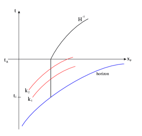
Figure 1: Space-time sketch of an inflationary cosmology. The vertical axis is time, the horizontal axis is physical distance. The inflationary phase lasts from $t_{i}$ until $t_{R}$, and it is during this period that the fluctuations we consider here exit the Hubble radius.

The formalism of stochastic inflationary dynamics describes the effect of modes exiting the Hubble radius on the evolution of the effective background field which is the full field coarse grained over the Hubble volume (see e.g. Laurence for a modern view on the formalism of stochastic inflation). In slight abuse of notation we will also denote the effective background field (and not just the full field) by $\varphi$. Taking into account the effects of modes crossing the Hubble radius which are now entering the sea of long wavelength modes, the equation of motion for $\varphi$ becomes

$${\ddot{\varphi}}+3H{\dot{\varphi}}+V^{\prime}(\varphi)\,=\,\frac{3}{2\pi}H^{3}\xi(t)\,,$$ (1)

which assumes that $H$ is approximately constant and where the prime denotes the derivative with respect to $\varphi$, and where $\xi(t)$ is a Gaussian random variable with unit variance which takes on different values in different Hubble patches. If $\xi(t)$ is positive, then the source term in (1) will drive $\varphi$ up the potential, but if $\xi(t)$ is negative, then the stochastic source will reinforce the classical force driving $\varphi$ down its potential.

The stochastic region of field space is defined to be the one for which the classical force term (the right hand side of (1) exceeds the classical force in magnitude, i.e.

$$\frac{3}{2\pi}H^{3}\,\geq\,|V^{\prime}(\varphi)|\,.$$ (2)

For example, for the simplest chaotic inflation model with potential

$$V(\varphi)\,=\,\frac{1}{2}m^{2}\varphi^{2}$$ (3)

the condition (2) becomes

$$|\frac{\varphi}{m_{pl}}|\,\geq\,\sqrt{4\pi}6^{1/4}\biggl{(}\frac{m_{pl}}{m}\biggr{)}^{1/2}\,,$$ (4)

where $m_{pl}$ is the reduced Planck mass defined in terms of Newton’s constant $G$ via $m_{pl}=(\sqrt{8\pi G})^{-1}$.

Note that for the normalization of the mass $m$ which is consistent with the observed amplitude of CMB anisotropies, the stochastic region of field space is far beyond the field values which influence the period of inflation which is observationally accessible to us. They do, however, correspond to energy densities which are still much lower than Planck densities.

III Back-Reaction of Long Wavelength Fluctuations

In early universe cosmology we usually consider a homogenous and isotropic background space-time and superimpose small amplitude cosmological fluctuations which are treated by linearizing the field equations about the background. The Einstein field equations, however, are highly nonlinear, and hence even at the classical level the fluctuations at second order influence the background. This is what we mean by back-reaction.

The expansion parameter for cosmological perturbation theory is the amplitude of the fluctuations which is set by the size of the observed CMB anisotropies and is of the order $10^{-5}$. Hence, the back-reaction effect of any given fluctuation mode is tiny (of the order $10^{-10}$). However, each fluctuation mode effects the background, and hence, for a long period of inflation the integrated effect of all of the modes can be important (see RHBrev1 for a review of back-reaction effects of long wavelength cosmological perturbations).

As mentioned in the introductory section, the back-reaction effect of sub-Hubble fluctuations is very small and approximately constant in time. On the other hand, the back-reaction of long wavelength modes shows secular growth due to the increasing phase space of super-Hubble modes.

How is it possible that super-Hubble scale modes can effect local physics? First of all, note that there is no causality obstacle. During inflation, the causal horizon (the forward light cone) is (almost) exponentially stretched compared to the Hubble radius. All modes we are considering have a wavelength which is smaller than the horizon. Secondly, note an analogy with black hole physics . If we throw a mass into a black hole, then the mass may have forever disappeared beyond the horizon, but the gravitational effects of this mass remain visible to the observer at infinity. In a similar way, the local gradients of a long wavelength cosmological fluctuation mode may decay exponentially, but the gravitational effects of this mode will persist and have a local effect.

The gravitational back-reaction formalism is as follows ABM . We begin with the full Einstein field equations

$$G_{\mu\nu}\,=\,8\pi GT_{\mu\nu}\,,$$ (5)

where $G_{\mu\nu}$ is the Einstein tensor and $T_{\mu\nu}$ is the energy-momentum tensor of matter. The background metric $g^{(0)}_{\mu\nu}(t)$ and matter $\varphi^{(0)}(t)$ obey these (nonlinear) equations. Next we introduce the linearized metric and matter fluctuations $\delta g_{\mu\nu}$ and $\delta\varphi$ which are both functions of space and time and which obey the linearized Einstein equations. However, the system of fields

$$g_{\mu\nu}(x,t)\, = \,g^{(0)}_{\mu\nu}(t)+\delta g_{\mu\nu}(x,t)\,$$

$$\varphi(x,t)\, = \,\varphi^{(0)}(t)+\delta\varphi(x,t)\,$$ (6)

does not satisfy the Einstein equations at second order.

If we are only interested in modifying the background at quadratic order (modifications of the fluctuations can be considered as well Patrick ) we need to introduce second order correction terms $g^{(2)}_{\mu\nu}(t)$ and $\varphi^{(2)}(t)$ to metric and matter. Adding these terms to the ansatz (III) for metric and matter, inserting into the Einstein equations (5), cancelling the linear terms using the linear fluctuation equations, moving all terms quadratic in the fluctuations to the right hand side, and taking the spatial average of the resulting equation yields an equation of motion for the corrected background metric

$$g^{(0,br)}_{\mu\nu}(t)\,=\,g^{(0)}_{\mu\nu}(t)+g^{(2)}_{\mu\nu}(t)$$ (7)

of the following form:

$$G_{\mu\nu}(g^{(0.br)})(t)\,=\,8\pi G\biggl{[}T^{(0)}_{\mu\nu}(\varphi^{(0)}(t))+\tau_{\mu\nu}(t)\biggr{]}\,,$$ (8)

where $\tau_{\mu\nu}(t)$ is quadratic in the cosmological fluctuations, and is called the “effective energy-momentum tensor of cosmological perturbations”. The effective energy momentum tensor is obtained by integrating over the contributions of all fluctuation (Fourier) modes. For the reasons explained above we are only interested in the contribution of the super-Hubble modes.

As background metric we take a spatially flat Friedmann-Robertson-Walker-Lemâitre metric given by the line element

$$ds^{2}\,=\,a(\eta)^{2}\bigl{(}d\eta^{2}-d\vec{x}^{2}\bigr{)}\,,$$ (9)

where $\eta$ is conformal time. To evaluate $\tau_{\mu\nu}$ we work in longitudinal (conformal-Newtonian) gauge in which (for single component matter without anisotropic stress) the line element is

$$ds^{2}\,=\,a(\eta)^{2}\biggl{[}(1+2\Phi)d\eta^{2}-(1-2\Phi)d\vec{x}^{2}\biggr{]}\,,$$ (10)

where $\Phi(x,t)$ is the relativistic gravitational potential Bardeen .

The metric and matter fluctuations are not independent. They are coupled via the Einstein constraint equations. In the background of a slowly rolling scalar field the connection is given by

$$\delta\varphi(k)\,=\,-\frac{2V}{V^{\prime}}\Phi(k)\,,$$ (11)

where the argument $k$ indicates that we are considering the Fourier modes of the fluctuations. The general expression for $\tau_{\mu\nu}$ contains many terms (see e.g. RHBrev1 for the full expression). However, for super-Hubble modes the terms containing spatial and temporal derivatives can be neglected, the latter since in an expanding universe the dominant mode of $\Phi$ is constant in time. The terms which survive give a contribution to the energy density of the form

$$\rho_{br}(t)\,\simeq\,\biggl{[}2\frac{V^{\prime\prime}V^{2}}{(V^{\prime})^{2}}-4V\biggr{]}\langle\Phi^{2}\rangle\,,$$ (12)

where $\langle\Phi^{2}\rangle$ is obtained by integrating over all of the super-Hubble modes. In the simple chaotic inflation model considered in ABM , the second term in (12) is larger in magnitude than the first, and hence the effective energy density of long wavelength cosmological perturbations is negative. We shall see that the same is true in the other models considered here. The effective pressure of cosmological perturbations is

$$p_{br}\,\simeq\,-\rho_{br}\,,$$ (13)

and hence long wavelength cosmological fluctuations effect the background geometry like a negative cosmological constant (with possible implications for a possible solution of the cosmological constant problem discussed in RHBrev1 ). The physical reason why long wavelength fluctuations act as a negative cosmological constant is easy to understand: a matter fluctuation (with positive matter energy density) leads to a potential well (negative gravitational energy density), and on super-Hubble scales the magnitude of the gravitational energy is larger than that of the matter energy, hence leading to a negative effective energy density. Since no terms with spatial and temporal gradients contribute, the equation of state of $\tau_{\mu\nu}$ has to be that of a cosmological constant.

An important question to ask Unruh is whether the effects of the contribution of super-Hubble modes to $\tau_{\mu\nu}$ are locally measurable. Returning to the black hole example, we note that there needs to be an observer (the observer at infinity) to measure the change in the mass of the black hole when some matter is thrown into it. In a similar way, a physical clock field is required in order to locally measure the effects of the long wavelength contribution to $\tau_{\mu\nu}$. For purely adiabatic fluctuations, the effect is equivalent Ghazal1 ; AW to a second order time-translation. However, in terms of a clock field $\chi$, the effects of the back-reaction of super-Hubble modes is physically measurable Ghazal2 , and it corresponds to a decrease in the local Hubble expansion rate Marozzi . From now on we will implicitly assume that we have a clock field present which plays the same role as the CMB plays in late time cosmology in setting the clock without producing curvature of space.

At this point we have established that stochastic effects lead (at least in half of space) to an increase in the energy density, whereas the back-reaction of super-Hubble modes leads to a decrease. In the following, we will compare the magnitude of these effects in various cosmological models.

IV Case 1: Power-Law Inflation

We first consider large field power-law inflation models with potential

$$V(\varphi)\,=\,\lambda m^{4-n}\varphi^{n}\,,$$ (14)

where $\lambda$ is a dimensionless constant and $m$ is a mass scale. This class of potentials include the simple chaotic inflation models with $n=2$ and $n=4$, and axion monodromy inflation models which $n$ can be a real number in the range $0<n<2$ axion . In the case of $n\neq 4$ we can without loss of generality set $\lambda=1$. However, sometimes it is convenient to keep $\lambda$ and instead replace $m$ by $m_{pl}$. With the first choice, the condition to obtain small density fluctuations is $m\ll m_{pl}$, in the second case $\lambda\ll 1$. Note that the region of slow roll inflation corresponds to trans-Planckian field value

$$|\varphi|\,>\,\alpha(n)m_{pl}\,,$$ (15)

where the $\alpha(n)$ is of the order $1$.

Taking the derivative of (14) to obtain the classical force and comparing with the stochastic force given by the right hand side of (1) we get the following field range for which the stochastic force dominates over the classical one:

$$|\varphi|\,>\,\biggl{(}2\pi\sqrt{3}n\biggr{)}^{f}\lambda^{-f/2}\biggl{(}\frac{m_{pl}}{m}\biggr{)}^{(2-\frac{1}{2}n)f}m_{pl}\,,$$ (16)

where the exponent $f$ is

$$f\,=\,\frac{1}{n/2+1}\,.$$ (17)

It is easy to see that in the case $n=2$ and $\lambda=1/2$ we recover the condition (2).

If we are in a region of space in which stochastic effects drive $\varphi$ up the potential, the increase in the potential energy over one Hubble time $H^{-1}$ is then given by

$$\Delta V\,\simeq\,\Delta\varphi V^{\prime}\,,$$ (18)

where

$$\Delta\varphi\,=\,\frac{H}{2\pi}$$ (19)

is the change in $\varphi$ over one Hubble time step (the coefficient in (19) is consistent with the coefficient of the stochastic term in (1)).

As discussed in the previous section, the back-reaction of super-Hubble modes leads to a negative contribution to the energy density which grows in time during a period of accelerated expansion since modes are exiting the Hubble radius and increasing the sea of infrared modes. In order to compare the change in the energy density due to back-reaction with the change due to stochastic evolution we need to evaluate the change in $\langle\Phi^{2}\rangle$ over a Hubble time, the same time interval considered above for the stochastic effect.

The starting point is the following expression for the contribution to $\langle\Phi^{2}\rangle$ from super-Hubble Fourier modes $\Phi(k)$:

$$\langle\Phi^{2}\rangle(t)\,=\,4\pi\int_{0}^{k_{H}(t)}k^{2}|\Phi(k)|^{2}dk\,,$$ (20)

where $k_{H}(t)$ is the comoving wavenumber corresponding to Hubble radius crossing at time $t$. The change in $\langle\Phi^{2}\rangle$ over one Hubble time is then given by

$$\Delta\langle\Phi^{2}\rangle\,=\,H^{-1}4\pi k_{H}^{2}|\Phi(k_{H}(t))|^{2}\frac{dk_{H}(t)}{dt}\,.$$ (21)

In the case of an exponentially expanding background we have

$$k_{H}(t)\,=\,a(t)H\,.$$ (22)

The corrections to this formula in the case of slow-roll inflation are negligible.

In the case of inflation, the value of $\Phi(k)$ at Hubble radius crossing is given by the vacuum initial conditions Mukh ; RHBrev . We use the relations

$$\zeta(k)\, \simeq \,\frac{2}{3}\frac{1}{1+w}\Phi(k)$$

$$\zeta(k)\, = \,z^{-1}v(k)\,,$$ (23)

which express the gravitational potential $\Phi$ in terms of the curvature fluctuation variable $\zeta$ (which is conserved in an expanding universe on super-Hubble scales), which is then in turn related to the canonical fluctuation variable $v$ Sasaki ; Mukh2 via the background variable $z$ which is given by

$$z\,=\,\frac{a{\dot{\varphi}^{(0)}}}{H}\,.$$ (24)

In the above, the equation of state parameter $w$ is the ratio of pressure to energy density. Using vacuum initial conditions for $v(k)$ we then obtain

$$\Delta\langle\Phi^{2}\rangle\,=\,\frac{9}{2}\pi H^{4}\frac{(\dot{\varphi}^{(0)})^{2}}{V^{2}}\,.$$ (25)

Inserting back into the expression (12) for the effective energy density of back-reaction we then obtain (after using the slow-roll equation of motion to replace $\dot{\varphi}^{(0)}$ in terms of $V^{\prime}$ and $V$):

$$\Delta\rho_{br}\,=\,\frac{\pi}{3}\biggl{[}V^{\prime\prime}V-2(V^{\prime})^{2}\biggr{]}m_{pl}^{-2}\,.$$ (26)

We are now able to compare the magnitude of the increase in energy density due to stochastic rolling up the potential with the decrease due to the increase in $\rho_{br}$. Combining the above equations (18), (19) and (26) yields

$$\frac{|\Delta\rho_{br}|}{\Delta V}\,=\,\frac{2\pi^{2}}{\sqrt{3}}\sqrt{\lambda}m^{2-\frac{1}{2}n}(n+1)\varphi^{\frac{1}{2}n-1}m_{pl}^{-1}\,.$$ (27)

Without loss of generality we can set $m=m_{pl}$ and represent the small slope of the potential (which is required in order for the cosmological fluctuations induced by inflation not to exceed the observational upper bound) by a small value $\lambda\ll 1$ of the coupling constant.

In the case $n=2$ it is clear from (27) that $|\Delta\rho_{br}|$ is smaller than $\Delta V$ for all field values. Hence, back-reaction cannot prevent eternal inflation. For $n>2$ there is a critical field value $\varphi_{c}$ beyond which $|\delta\rho_{br}|$ exceeds $\Delta V$:

$$\varphi_{c}\,=\,\biggl{(}\frac{\sqrt{3}}{2\pi^{2}}\frac{1}{n+1}\biggr{)}^{\frac{1}{n/2-1}}\lambda^{-\frac{1}{n-2}}m_{pl}$$ (28)

which corresponds to trans-Planckian energy densities. Once again, back-reaction cannot prevent eternal inflation. Finally, for $n<2$ the exponents reverse sign and the condition for $\Delta\rho_{br}$ to dominate becomes an upper bound for $|\varphi|$:

$$|\varphi|^{\tilde{n}}\,<\,\frac{1}{3}\lambda^{1/2}(n+1)m_{pl}^{\tilde{n}}\,,$$ (29)

where ${\tilde{n}}\equiv 1-n/2$. This is not the field range for inflation.

In conclusion, we find that in no version of simple power law inflation models back-reaction of long wavelength fluctuations can prevent eternal inflation.

V Case 2: Starobinsky Inflation

Starobinsky’s initial model of exponential expanding space was based on a higher derivative gravitational Lagrangian Starob0 . After a conformal transformation, it corresponds to Einstein gravity in the presence of a scalar matter field $\varphi$ with exponential potential

$$V(\varphi)\,=\,A\bigl{(}1-e^{-b\varphi}\bigr{)}^{2}\,,$$ (30)

where the $A\ll m_{pl}^{4}$ and $b\sim m_{pl}^{-1}$. Such potentials also arise in chaotic inflation in supergravity GL .

The region of inflation once again corresponds to trans-Planckian field values where the potential energy is approximately given by $A$. As in the case of power law inflation discussed in the previous section, we first determine the field range where stochastic effects dominate. Demanding that the stochastic force amplitude exceeds the classical force yields the condition

$$\varphi\,>\,b^{-1}{\rm ln}\biggl{[}\frac{3}{4\pi}\biggl{(}\frac{1}{3}\biggr{)}^{3/2}\biggl{(}\frac{A}{m_{pl}^{4}}\biggr{)}^{1/2}(bm_{pl})^{-1}\biggr{]}\,.$$ (31)

Now we can turn to a comparison of the increase in potential energy due to stochastic rolling up the potential to the change in the energy density of back-reaction. Making use of (18) and (19), expressing $H$ in terms of $V$, and making the approximation $V\simeq A$ we obtain

$$\Delta V\,\simeq\,\frac{1}{\sqrt{3}\pi}bA^{3/2}e^{-b\varphi}m_{pl}^{-1}\,.$$ (32)

On the other hand, from (12) and (25), the change in the energy density of back-reaction is given by

$$\Delta\rho_{br}\simeq\,-\frac{2\pi}{3}A^{2}b^{2}e^{-b\varphi}m_{pl}^{-2}\,.$$ (33)

The ratio is

$$\frac{|\Delta\rho_{br}|}{\Delta V}\,=\,\frac{2\sqrt{3}}{3}\pi^{2}A^{1/2}bm_{pl}^{-1}$$ (34)

which is much smaller than unity for the values of $A$ and $b$ which need to be chosen to get successful inflation. Hence, we conclude that also in Starobinksy inflation back-reaction terms are too weak to prevent eternal inflation.

VI Case 3: Cyclic Ekpyrotic Scenario

Finally, we turn to the “dark energy phase” of the cyclic Ekpyrotic scenario. The Ekpyrotic scenario is an alternative to inflation for producing the observed inhomogeneities and anisotropies Ekp . It is based on the Horava-Witten scenario of heterotic M-theory Horava , a higher dimensional model. At the effective field theory level it reduces to the theory of a scalar field (in the higher dimensional picture it corresponds to the separation of parallel branes) coupled to Einstein gravity. The potential of the scalar field is argued to be a negative exponential. This setup leads to a bouncing cosmology. According to the Ekpyrotic scenario, the universe begins in a phase of contraction in which the scalar field is rolling down the potential. Since the potential is negative, one obtains an equation of state with $w\gg 1$, where the equation of state parameter $w$ is the ratio of energy density and pressure. Once the scalar field drops below $\varphi=0$ (which corresponds to the brane separation approaching the string scale), a cosmological bounce is assumed to take place during which regular matter and radiation are produced, leading to a Standard Big Bang phase of expansion during which $\varphi$ climbs back up the potential (while being a subdominant form of matter). Cosmological fluctuations are created during the phase of contraction. As long as an almost massless entropy field is present (and this completely natural from the higher dimensional point of view BBP ), an almost scale-invariant spectrum of curvature perturbations is generated Notari ; Turok ; Creminelli ; NewEkp .

By introducing a slight lift of the potential, i.e. by choosing

$$V(\varphi)\,=\,C-V_{0}e^{-a\varphi}\,,$$ (35)

the Ekpyrotic scenario becomes “cyclic” ST . Once $\varphi$ during the phase of cosmic expansion reaches values with $V(\varphi)>0$, a period of accelerated expansion will start. The scenario thus includes dark energy. Based on the classical equation of motion for $\varphi$ we would conclude that $\varphi$ will eventually turn around and start to decrease. This leads to a phase of contraction: the Ekpyrotic scenario has become cyclic. Figure 2 presents a sketch of space-time in the Ekpyrotic scenario. The vertical axis is time, the horizontal is comoving distance. The bounce time is taken to be $t=0$. The Hubble radius decreases very fast before the bounce and then slowly increases in the Standard Big-Bang phase after the bounce. For the cyclic Ekpyrotic scenario to work the way it is meant to, the constant $C$ corresponds to the currently observed cosmological constant, whereas the value of $V_{0}$ corresponds typically to a very high scale (e.g. the energy scale of Grand Unification). Also, the value of $a$ will be given by the inverse string scale.

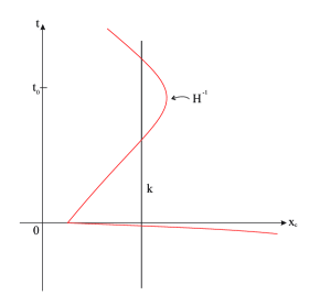
Figure 2: Space-time sketch of the cyclic Ekpyrotic scenario. The vertical axis is time, the horizontal is comoving physical distance. Fluctuations are generated during the phase of contraction for $t<0$. The bounce occurs at $t=0$ and is followed by an expanding phase. Close to the present time, we enter the dark energy phase driven by the term $C$ in the potential (35). The fluctuations which exit the Hubble radius during this phase are not vacuum perturbations, but the evolved ones and have a much larger amplitude than vacuum fluctuations would have.

A question to ask is whether stochastic effects analogous to the ones which drive stochastic eternal inflation will lead to an eternal stochastic growth of $\varphi$ in the Ekpyrotic scenario, thus leading to an “Ekpyrotic landscape”. Intuitively we would not expect this to happen since the stochastic effects are highly suppressed in the dark energy phase (since $C<<<m_{pl}^{4}$) whereas the cosmological fluctuations (and hence their back-reaction effects) are not suppressed compared to the case of inflation. In fact, when the fluctuations exit the Hubble radius in the accelerating phase, they are not in the vacuum state, unlike in the case of Starobinsky inflation. Hence, the formula for the energy density of back-reaction is different. These effects lead to an enhancement of the back-reaction “force” compared to the stochastic one. In the following we will show that these expectations are indeed borne out.

The value of $\varphi$ which corresponds to $V=0$ will be denoted by $\varphi_{0}$ and is given by

$$e^{-a\varphi_{0}}\,=\,\frac{C}{V_{0}}\,.$$ (36)

For field values significantly larger than $\varphi_{0}$ we can approximate the value of the potential by $V=C$. In this case, the increase in potential energy while rolling up the potential for one Hubble time is given by

$$\Delta V\,\simeq\,\frac{1}{2\pi}\biggl{(}\frac{1}{3}\biggr{)}^{1/2}C^{3/2}am_{pl}^{-1}e^{-a\delta\varphi}\,,$$ (37)

where

$$\varphi\,\equiv\,\varphi_{0}+\delta\varphi\,.$$ (38)

Turning to the evaluation of the change in the energy density due to back-reaction, it is important to note that the fluctuations which are exiting the Hubble radius during the dark energy phase are not the vacuum ones, but the ones which have evolved and have produced the structure which we see on large scales. We hence have

$$\Delta\langle\Phi^{2}\rangle\,\sim\,1$$ (39)

and hence from (12)

$$\Delta\rho_{br}\,=\,2\biggl{[}\frac{V^{\prime\prime}V^{2}}{(V^{\prime})^{2}}-2V\biggr{]}\,.$$ (40)

Inserting the form of the Ekpyrotic potential and considering large field values we find

$$\Delta\rho_{br}\,\sim\,-2Ce^{a\delta\varphi}\,.$$ (41)

Comparing (37) and (41) we find

$$\frac{|\Delta\rho_{br}|}{\Delta V}\,=\,4\pi\sqrt{3}\frac{a^{-1}m_{pl}}{C^{1/2}}e^{2a\delta\varphi}\,.$$ (42)

Since the scale $C$ corresponds to the current dark energy scale, the coefficient in front of the exponential in the above equation is many orders of magnitude larger than $1$. Hence we conclude that in the cyclic Ekpyrotic scenario back-reaction prevents the stochastic growth of $\varphi$ and that there hence is no eternal expansion in the late time dark energy phase for this model.

VII Conclusions and Discussion

Stochastic effects will lead to the effective scalar field climbing up the potential in some regions of space. This leads to an increase in the energy density. On the other hand, the back-reaction of fluctuations which have already exited the Hubble radius will lead to a decrease in the effective energy density. In this paper we have compared the magnitude of the two effects in various cosmologies with an accelerating phase.

We have shown that for both power-law and Starobinsky inflation that strength of the back-reaction effect is too weak to prevent the stochastic growth of $\varphi$ and hence does not cut off eternal inflation. On the other hand, the back-reaction of fluctuations in the dark energy phase of the cyclic Ekpyrotic scenario greatly overwhelms the increase in energy due to stochastic dynamics, and hence no eternal expansion in the late time dark energy phase for the Ekpyrotic scenario is generated.

It is worth mentioning that besides the calculations done in this paper, we have also looked into generalizations of them. The first idea was to consider that $N$ Hubble times could pass so that more modes could leave the Hubble radius and the back-reaction effect would be increased to the point that even power-law and Starobinsky models could not have eternal inflation. On the other hand, this would also enhance the stochastic effect since the total $\Delta\varphi$ would be larger. At the end, we found that the number $N$ for which back-reaction starts to overwhelm the stochastic effect would be unreasonably large in the setup of inflation.

Furthermore, one could notice that (12) assumes the slow-roll equation of motion for the inflaton field. However, since the field is rolling under the influence of the stochastic force, this formula should be generalized. Therefore, we have also treated all the scenarios discussed in this paper using the generalization of the effective energy density of back-reaction obtained when considering the correct equations of motion. We found that 1) for power-law inflation, there are field regions in which the back-reaction effective energy density becomes positive instead of negative, thus being completely unable to prevent eternal inflation; 2) for Starobinsky inflation and for the Ekpyrotic scenario, the conclusions remain the same as the ones obtained here.

It is also worth while commenting on the relation of our work to the conclusions reached in ABM . In those works, the question addressed was what the absolute magnitude of the back-reaction energy density is assuming that slow-roll inflation starts at some field value $\varphi_{i}$ and lasts until $\varphi\sim m_{pl}$. In the case of a potential $V(\varphi)=\frac{1}{2}m^{2}\varphi^{2}$ it was found that if $\varphi_{i}>m^{-1/3}$ (in Planck units) then the total energy in the back-reacting infrared modes becomes larger than the background energy density. In that work, however, the effects of the stochastic noise leading to an increase in $\varphi$ was not considered. Thus, the questions considered in ABM and in this paper are complementary.