Gibbs measures and free energies of Ising-Vannimenus Model on the Cayley tree

Abstract.

In this paper, we consider Ising-Vannimenus model on a Cayley tree for order two with competing nearest-neighbor, prolonged next-nearest neighbor interactions. We stress that the mentioned model was investigated only numerically, without rigorous (mathematical) proofs. One of the main point of this paper is to propose a measure-theoretical approach the considered model. We find certain conditions for the existence of Gibbs measures corresponding to the model. Then we establish the existence of the phase transition. Moreover, the free energies of the found Gibbs measures are calculated. Mathematics Subject Classification: 46S10, 82B26, 12J12, 39A70, 47H10, 60K35.
Key words: Ising model; Gibbs measure, phase transition, Free energy.

1. introduction

Gibbs measure is ne of the central objects of equilibrium statistical mechanic, a branch of probability theory that takes its origin from Boltzmann [2]. Also, one of the main problems of the Statistical Physics is to describe all Gibbs measures corresponding to the given Hamiltonian. It is well known that such measures form a nonempty convex compact subset in the set of all probabilistic measures. The purpose of this paper is to investigate Gibbs measures of the Ising model [39] with ternary prolonged and nearest neighbor interactions on Bethe lattice of order two and to describe its extreme elements (pure phases). In [16], we have studied phase diagram and extreme Gibbs measures of the Ising model on a Cayley tree in the presence of competing binary and ternary interactions. In [18], we have obtained the extreme Gibbs measures of the Ising-Vannimenus (IV) model [39] without proof a number of theorems related to the description of the general structure of extreme Gibbs distributions of the Ising model on a Cayley. we studied Gibbs states (phases) that correspond in probability theory to what are called Markov chains with memory length 2 by using the method in [18]. In this paper, we combine the results obtained in [17] and [18]. In [32], the authors study the existence of $p$-adic quasi Gibbs measures by means of investigation of the obtained equations via methods of $p$-adic analysis. Note that the methods used in [32] are not valid in a real setting. Therefore, in this paper we will give a rigorous description of Gibbs measures corresponding to Ising-Vannimnus in the real setting.

Recently, Ganfoldo et al [21] have obtained some explicit formulae of the free energies (and entropies) according to boundary conditions (b.c.) for the Ising model on the Cayley tree. Also, Ganfoldo et al [19] study the Ising model on a Cayley tree. They show that a wide class of new extreme Gibbs states is exhibited.

Until now, many researchers have investigated Gibbs measure with memory one over Cayley tree. In this paper, we consider Ising model on a Cayley tree for order two with competing nearest-neighbor, prolonged next-nearest neighbor interactions. We stress that the mentioned model was investigated only numerically, without rigorous (mathematical) proofs. We propose a rigorous measure-theoretical approach to investigate a Ising-Vanniminus model on a Cayley tree of order two. We find certain conditions for the existence of Gibbs measures corresponding to the model. Then we establish the existence of the phase transition. We investigate the behavior of free energy at these new transition points. We present some explicit formulae of the free energies corresponding to boundary conditions for the Ising-Vannimenus model on the Cayley tree of order two.

2. Preliminaries

2.1. Vannimenus Model with competing interactions on Cayley tree

A Cayley tree $\Gamma^{k}$ of order $k\geq 1$ is an infinite tree, i.e., a graph without cycles with exactly $k+1$ edges issuing from each vertex. Let us denote the Cayley tree as $\Gamma^{k}=(V,\Lambda,i)$ where $V$ is the set of vertices of $\Gamma^{k}$, $\Lambda$ is the set of edges, and $i$ the incidence function which associates with each edge $l\in L$ its endpoints. Two vertices $x$ and $y$, $x,y\in V$ are called nearest-neighbors if there exists an edge $l\in\Lambda$ connecting them, which is denoted by $l=<x,y>$. The distance $d(x,y),x,y\in V$, on the Cayley tree $\Gamma^{k}$, is the number of edges in the shortest path from $x$ to $y$. Two vertices $x,y\in V^{0}$ are called the next-nearest-neighbours if $d(x,y)=2$. Next-nearest-neighbour vertices $x$ and $y$ are called prolonged next-nearest-neighbours if they belong to the same branch which is denoted by $\widetilde{>x,y<}$. Let spin variables $\sigma(x),x\in V,$ take values $\pm 1$. Then the Vannimenus model with competing nearest-neighbours and next-nearest-neighbours binary interactions is defined by the following Hamiltonian

(2.1) $$H(\sigma)=-J_{p}\sum_{\widetilde{>x,y<}}\sigma(x)\sigma(y)-J\sum_{<x,y>}\sigma(x)\sigma(y),$$

where the sum in the first term ranges all prolonged next-nearest-neighbours and the sum in the second term ranges all nearest-neighbours. Here $J_{p},J\in{R}$ are coupling constants.

The distance $d(x,y),x,y\in V$, on the Cayley tree $\Gamma^{k}$, is the number of edges in the shortest path from $x$ to $y$. For a fixed $x^{0}\in V$ we set

$$W_{n}=\{x\in V|d(x,x^{0})=n\},\\ V_{n}=\{x\in V|d(x,x^{0})\leq n\}$$

and $L_{n}$ denotes the set of edges in $V_{n}$. The fixed vertex $x^{0}$ is called the $0$-th level and the vertices in $W_{n}$ are called the $n$-th level and for $x\in W_{n}$ let

$$S(x)=\{y\in W_{n-1}|d(x,y)=1\},$$

be the set of direct successors of $x$.

Note in [39] it is assumed that $J>0$ and $J_{p}<0.$ Below we consider model (1) with arbitrary sign of the coupling constants.

As usual, one can introduce the notions of Gibbs distribution of this model, limiting Gibbs distribution, pure phase ( extreme Gibbs distribution ), etc (see [10], [12],[23], [33]).

3. Translation-invariant Gibbs measures of the Ising-Vannimenus model

In this section we define a notion of Gibbs measure corresponding to the Ising-Vannimenus model in a general setting, i.e. for arbitrary nearest-neighbor models (see [39]). We propose a new kind of construction of Gibbs measures corresponding to the Ising-Vannimenus model.

Let $\Phi=\{-1,+1\}$ ($\Phi$ is called a state space) and is assigned to the vertices of the tree $\Gamma^{k}_{+}=(V,\Lambda)$. A configuration $\sigma$ on $V$ is then defined as a function $x\in V\to\sigma(x)\in\Phi$; in a similar manner one defines configurations $\sigma_{n}$ and $\omega$ on $V_{n}$ and $W_{n}$, respectively. The set of all configurations on $V$ (resp. $V_{n}$, $W_{n}$) coincides with $\Omega=\Phi^{V}$ (resp. $\Omega_{V_{n}}=\Phi^{V_{n}},\ \ \Omega_{W_{n}}=\Phi^{W_{n}}$). One can see that $\Omega_{V_{n}}=\Omega_{V_{n-1}}\times\Omega_{W_{n}}$. Using this, for given configurations $\sigma_{n-1}\in\Omega_{V_{n-1}}$ and $\omega\in\Omega_{W_{n}}$ we define their concatenations by

$$(\sigma_{n-1}\vee\omega)(x)=\left\{\begin{array}[]{ll}\sigma_{n-1}(x),\ \ \textrm{if}\ \ x\in V_{n-1},\\ \omega(x),\ \ \ \ \ \ \textrm{if}\ \ x\in W_{n}.\\ \end{array}\right.$$

It is clear that $\sigma_{n-1}\vee\omega\in\Omega_{V_{n}}$.

For the Ising model with spin values in $\Phi=\{-1,+1\}$, the relevant Hamiltonian with competing nearest-neighbor, prolonged next-nearest-neighbor and two-level triple interactions has the form

(3.1) $$H(\sigma)=-J_{p}\sum\limits_{\widetilde{>x,y<}}\sigma(x)\sigma(y)-J\sum\limits_{<x,y>}\sigma(x)\sigma(y),$$

Assume that ${\mathbf{h}}:V\setminus\{x^{(0)}\}\to\ \mathbb{R}$ is a mapping, i.e.

$${\mathbf{h}}_{xy,\sigma(x)\sigma(y)}=(h_{xy,++},h_{xy,+-},h_{xy,-+},h_{xy,--}),$$

where ${\mathbf{h}}_{xy,\sigma(x)\sigma(y)}\in\mathbb{R}$ ($\sigma(x),\sigma(y)\in\{-1,+1\}$) and $x,y\in V\setminus\{x^{(0)}\}$.

Now, we define Gibbs measure with memory of length 2 over Cayley tree.

(3.2) $$\mu_{n,h}(\sigma)=\frac{1}{Z_{n}}\exp[-\beta H_{n}(\sigma)+\sum_{x\in W_{n-1}}\sum_{y\in S(x)}\sigma(x)\sigma(y){\mathbf{h}}_{xy,\sigma(x)\sigma(y)}].$$

Here, as before, $\beta=\frac{1}{kT}$ and $\sigma_{n}:x\in V_{n}\to\sigma_{n}(x)$ and $Z_{n}$ is the corresponding to partition function

$$Z_{n}=\sum\limits_{\sigma_{n}\in\Omega_{V_{n}}}\exp[-\beta H(\sigma_{n})+\sum_{x\in W_{n-1}}\sum_{y\in S(x)}\sigma(x)\sigma(y){\mathbf{h}}_{xy,\sigma(x)\sigma(y)}].$$

In this paper, we are interested in a construction of an infinite volume distribution with given finite-dimensional distributions. More exactly, we would like to find a probability measure $\mu$ on $\Omega$ which is compatible with given ones $\mu_{{\mathbf{h}}}^{(n)}$, i.e.

(3.3) $$\mu(\sigma\in\Omega:\sigma|_{V_{n}}=\sigma_{n})=\mu^{(n)}_{{\mathbf{h}}}(\sigma_{n}),\ \ \ \textrm{for all}\ \ \sigma_{n}\in\Omega_{V_{n}},\ n\in{\mathbb{N}}.$$

The consistency condition for $\mu_{n,h}(\sigma_{n})$, $n\geq 1$ is

(3.4) $$\sum_{\omega\in\Omega_{W_{n}}}\mu^{(n)}_{{\mathbf{h}}}(\sigma_{n-1}\vee\omega)=\mu^{(n-1)}_{{\mathbf{h}}}(\sigma_{n-1}),$$

for any $\sigma_{n-1}\in\Omega_{V_{n-1}}$.

This condition according to the theorem implies the existence of a unique measure $\mu_{{\mathbf{h}}}$ defined on $\Omega$ with a required condition (3.3). Such a measure $\mu_{{\mathbf{h}}}$ is said to be Gibbs measure corresponding to the model. Note that more general theory of measures has been developed in [23].

For $\sigma_{n-1}\in V_{n-1}$ and $\eta\in W_{n}$, we can define the Hamiltonian as following;

$$H_{n}(\sigma_{n-1}\vee\eta) = -J\sum\limits_{<x,y>\in V_{n-1}}\sigma(x)\sigma(y)-J\sum\limits_{x\in W_{n-1}}\sum\limits_{y\in S(x)}\sigma(x)\eta(y)$$

$$-J_{p}\sum\limits_{>x,y<\in V_{n-1}}\sigma(x)\sigma(y)-J_{p}\sum\limits_{x\in W_{n-2}}\sum\limits_{z\in S^{2}(x)}\sigma(x)\eta(z)$$

$$= H_{n}(\sigma_{n-1})-J\sum\limits_{x\in W_{n-1}}\sum\limits_{y\in S(x)}\sigma(x)\eta(y)-J_{p}\sum\limits_{x\in W_{n-2}}\sum\limits_{z\in S^{2}(x)}\sigma(x)\eta(z).$$

Lemma 3.1.

If $\frac{\mathbf{a}}{\mathbf{b}}=\frac{N_{1}}{N_{2}}$, $\frac{\mathbf{a}}{\mathbf{c}}=\frac{N_{1}}{N_{3}}$ and $\frac{\mathbf{a}}{\mathbf{d}}=\frac{N_{1}}{N_{4}}$, then there exists $D\in\mathbb{R}$ such that $\mathbf{a}=DN_{1}$, $\mathbf{b}=DN_{2}$, $\mathbf{c}=DN_{3}$ and $\mathbf{d}=DN_{4}$.

Proof.

Due to statement of Lemma, we have
$\mathbf{a}=DN_{1}$, $\mathbf{b}=DN_{2}$,
$\mathbf{a}=D_{1}N_{1}$, $\mathbf{c}=D_{1}N_{3}$,
$\mathbf{a}=D_{2}N_{1}$, $\mathbf{d}=D_{2}N_{4}$. Therefore, from $\frac{\mathbf{a}}{\mathbf{b}}=\frac{DN_{1}}{D_{1}N_{2}}=\frac{N_{1}}{N_{2}}$, $D=D_{1}$. Similarly, from $\frac{\mathbf{a}}{\mathbf{d}}=\frac{DN_{1}}{D_{2}N_{4}}=\frac{N_{1}}{N_{4}}$, $D=D_{2}$. So, $D=D_{1}=D_{2}$. ∎

Theorem 3.2.

Probability distributions $\mu_{n}(\sigma_{n})$, $n=1,2,...,$ in (3.2) are compatible iff for any $x,y\in V$ the following equations hold:

(3.6) $$e^{h_{xy,++}+h_{xy,-+}} = \prod\limits_{z\in S(y)}\frac{\exp[{\mathbf{h}}_{yz,++}](ab)^{2}+\exp[-{\mathbf{h}}_{yz,+-}]}{\exp[{\mathbf{h}}_{yz,++}]a^{2}+\exp[-{\mathbf{h}}_{yz,+-}]b^{2}}$$

$$e^{h_{xy,--}+h_{xy,+-}} = \prod\limits_{z\in S(y)}\frac{\exp[-{\mathbf{h}}_{yz,-+}]+\exp[{\mathbf{h}}_{yz,--}](ab)^{2}}{\exp[-{\mathbf{h}}_{yz,-+}]b^{2}+\exp[{\mathbf{h}}_{yz,--}]a^{2}}$$

$$e^{h_{xy,++}+h_{xy,+-}} = \prod\limits_{z\in S(y)}\frac{\exp[{\mathbf{h}}_{yz,++}](ab)^{2}+\exp[{\mathbf{h}}_{yz,+-}]]}{\exp[-{\mathbf{h}}_{yz,-+}]b^{2}+\exp[{\mathbf{h}}_{yz,--}]a^{2}},$$

where $a=\exp(\beta J)$ and $b=\exp(\beta J_{p})$.

Proof.

Necessity. From the equation (3.4), we have

$$L_{n}\sum\limits_{\eta\in\Omega_{W_{n}}}\exp[-\beta H_{n}(\sigma_{n-1}\vee\eta)+\sum\limits_{x\in W_{n-1}}\sum\limits_{y\in S(x)}\sigma(x)\sigma(y){\mathbf{h}}_{xy,\sigma(x)\sigma(y)}]$$

$$= \exp[-\beta H_{n}(\sigma_{n-1})+\sum\limits_{x\in W_{n-2}}\sum\limits_{y\in S(x)}\sigma(x)\sigma(y){\mathbf{h}}_{xy,\sigma(x)\sigma(y)}],$$

where $L_{n}=\frac{Z_{n-1}}{Z_{n}}$.

From the equation (3), we have

$$L_{n}\sum\limits_{\eta\in\Omega_{W_{n}}}\exp[-\beta H_{n}(\sigma_{n-1})-\beta J\sum\limits_{x\in W_{n-1}}\sum\limits_{y\in S(x)}\sigma(x)\eta(y)$$

$$- \beta J_{p}\sum\limits_{x\in W_{n-2}}\sum\limits_{z\in S^{2}(x)}\sigma(x)\eta(z)+\sum\limits_{x\in W_{n-1}}\sum\limits_{y\in S(x)}\sigma(x)\sigma(y){\mathbf{h}}_{xy,\sigma(x)\sigma(y)}]$$

$$= \exp[-\beta H_{n}(\sigma_{n-1})+\sum\limits_{x\in W_{n-2}}\sum\limits_{y\in S(x)}\sigma(x)\sigma(y){\mathbf{h}}_{xy,\sigma(x)\sigma(y)}],$$

$$L_{n}\prod\limits_{x\in W_{n-2}}\prod\limits_{y\in S(x)}\prod\limits_{z\in S(y)}\sum\limits_{\eta(z)\in\{\mp 1\}}\exp[\sigma(y)\eta(z){\mathbf{h}}_{yz,\sigma(y)\eta(z)}+\beta\eta(z)(J\sigma(y)+J_{p}\sigma(x))]$$

$$= \prod\limits_{x\in W_{n-2}}\prod\limits_{y\in S(x)}\exp[\sigma(x)\sigma(y){\mathbf{h}}_{xy,\sigma(x)\sigma(y)}].$$

Let us fix $<x,y>$ and considering all values of $\sigma(x),\sigma(y)\in\{-1,+1\}$. Then from (3), we have

(3.8) $$e^{h_{xy,++}+h_{xy,-+}}=\prod\limits_{z\in S(y)}\frac{\sum\limits_{\eta(z)\in\{\mp 1\}}\exp[\eta(z)({\mathbf{h}}_{yz,+\eta(z)}+\beta(J+J_{p}))]}{\sum\limits_{\eta(z)\in\{\mp 1\}}\exp[\eta(z)({\mathbf{h}}_{yz,+\eta(z)}+\beta(J-J_{p}))]}$$

(3.9) $$e^{h_{xy,--}+h_{xy,+-}}=\prod\limits_{z\in S(y)}\frac{\sum\limits_{\eta(z)\in\{\mp 1\}}\exp[-\eta(z)({\mathbf{h}}_{yz,-\eta(z)}+\beta(J+J_{p}))]}{\sum\limits_{\eta(z)\in\{\mp 1\}}\exp[-\eta(z)({\mathbf{h}}_{yz,-\eta(z)}-\beta(-J+J_{p}))]}$$

(3.10) $$e^{h_{xy,++}+h_{xy,+-}}=\prod\limits_{z\in S(y)}\frac{\sum\limits_{\eta(z)\in\{\mp 1\}}\exp[\eta(z)({\mathbf{h}}_{yz,+\eta(z)}+\beta(J+J_{p}))]}{\sum\limits_{\eta(z)\in\{\mp 1\}}\exp[-\eta(z)({\mathbf{h}}_{yz,-\eta(z)}-\beta(-J+J_{p}))]}$$

These equations imply the desired equations. This completes the proof.

Sufficiency: Now assume that the system of equations in (3.6) is valid, then from Lemma 3.1 we get

$$e^{\sigma(x)\sigma(y)h_{xy,\sigma(x)\sigma(y)}}D(x,y)=\prod\limits_{z\in S(y)}\sum\limits_{\eta(z)\in\{\mp 1\}}\exp[\sigma(y)\eta(z){\mathbf{h}}_{yz,\sigma(y)\eta(z)}+\beta\eta(z)(J\sigma(y)+J_{p}\sigma(x))].$$

From the last equality, one can get

$$\prod\limits_{x\in W_{n-2}}\prod\limits_{y\in S(x)}D(x,y)e^{\sigma(x)\sigma(y)h_{xy,\sigma(x)\sigma(y)}}$$

$$= \prod\limits_{x\in W_{n-2}}\prod\limits_{y\in S(x)}\prod\limits_{z\in S(y)}\sum\limits_{\eta(z)\in\{\mp 1\}}e^{[\sigma(y)\eta(z){\mathbf{h}}_{yz,\sigma(y)\eta(z)}+\beta\eta(z)(J\sigma(y)+J_{p}\sigma(x))]}.$$

Multiply both sides of the equation (3) by $e^{-\beta H_{n-1}(\sigma)}$ and denoting

$$U_{n}=\prod\limits_{x\in W_{n-2}}\prod\limits_{y\in S(x)}D(x,y),$$

we have from (3),

$$U_{n-1}e^{-\beta H_{n-1}(\sigma)+\sum\limits_{x\in W_{n-2}}\sum\limits_{y\in S(x)}\sigma(x)\sigma(y)h_{xy,\sigma(x)\sigma(y)}}$$

$$= \prod\limits_{x\in W_{n-2}}\prod\limits_{y\in S(x)}\prod\limits_{z\in S(y)}e^{-\beta H_{n-1}(\sigma)}\sum\limits_{\eta(z)\in\{\mp 1\}}e^{[\sigma(y)\eta(z){\mathbf{h}}_{yz,\sigma(y)\eta(z)}+\beta\eta(z)(J\sigma(y)+J_{p}\sigma(x))]}.$$

Therefore, we get

$$U_{n-1}Z_{n-1}\mu_{n-1}(\sigma)=\sum\limits_{\eta}e^{-\beta H_{n}(\sigma\vee\eta)+\sum\limits_{x\in W_{n-2}}\sum\limits_{y\in S(x)}\sigma(x)\sigma(y)h_{xy,\sigma(x)\sigma(y)}}$$

(3.12) $$U_{n-1}Z_{n-1}\mu_{n-1}(\sigma)=Z_{n}\sum\limits_{\eta}\mu_{n}(\sigma\vee\eta).$$

As $\mu_{n}$ ($n\geq 1$) is a probability measures, i.e.

$$\sum\limits_{\sigma\in\{-1,+1\}^{V_{n-1}}}\mu_{n-1}(\sigma)=\sum\limits_{\sigma\in\{-1,+1\}^{V_{n-1}}}\sum\limits_{\eta\in\{-1,+1\}^{W_{n}}}\mu_{n}(\sigma\vee\eta)=1.$$

From these equalities and the equation (3.12) we have $Z_{n}=U_{n-1}Z_{n-1}$.

This with the equation (3.12) implies that (3.4) holds. ∎

According to Theorem 3.2 the problem of describing the Gibbs measures is reduced to the descriptions of the solutions of the functional equations (3.6).

4. The existence of phase transition

Below we produce restrict ourselves to the case

(4.1) $$h_{xy,++}=h_{xy,-+}=h_{1}\mbox{ and }h_{xy,--}=h_{xy,+-}=h_{2}.$$

Denoting Since $\ln u_{1}=h_{xy,++}=h_{xy,-+}$ and $\ln u_{2}=h_{xy,--}=h_{xy,+-}$ for any $x,y\in V$, one can produce

(4.2) $$u_{1}^{2}=\bigg{(}\frac{a^{2}b^{2}u_{1}u_{2}+1}{a^{2}u_{1}u_{2}+b^{2}}\bigg{)}^{2}=u_{2}^{2},$$

where $a=e^{\beta J}$ and $b=e^{\beta J_{p}}$. Hence $u_{1}=u_{z}$. Let $u_{1}=u_{2}=u$, we have

$$u=\frac{(ab)^{2}u^{2}+1}{a^{2}u^{2}+b^{2}}.$$

Let us consider a non-linear function:

(4.3) $$f(u)=\frac{(ab)^{2}u^{2}+1}{a^{2}u^{2}+b^{2}}.$$

Let us substitute as $c=a^{2}$ and $d=b^{2}$, then we have a non-linear function as;

(4.4) $$g(u)=\frac{cdu^{2}+1}{cu^{2}+d}.$$

The analysis of the solution of the equations (3.6) is rather trick. In this subsection, we will study the translation-invariant solutions, where $h_{xy}=h$ is constant $\forall x,y\in V.$ Let us consider

(4.5) $$u=\frac{cdu^{2}+1}{cu^{2}+d},$$

where $u=e^{h}$. Note that if there is more than one positive solution for the equation (4.5), then we have more than one translation-invariant Gibbs measure corresponding to the solution of the equation (4.5). Fixed points $u$ correspond to Markov chain Gibbs measures [41] (also splitting Gibbs measures or Bethe Gibbs measures).

Proposition 4.1.

The equation $u=\frac{cdu^{2}+1}{cu^{2}+d}$ has one solution if either $c\leq 1$ or $d<3$. If $d\geq 3$ then there exist $\eta_{1}(d)$, $\eta_{2}(d)$ with $0<\eta_{1}(d)<\eta_{2}(d)$ such that equation (4.5) has three solutions if $\eta_{1}(d)<c<\eta_{2}(d)$ and has two solutions if either $\eta_{1}(d)=c$ or $\eta_{2}(d)=c$.

Proof.

Denote

$$g(u)=\frac{cdu^{2}+1}{cu^{2}+d}.$$

We have

$$g^{\prime}(u)=\frac{2c(-1+d)(1+d)u}{\left(d+cu^{2}\right)^{2}}$$

$$g^{\prime\prime}(u)=-\frac{2c(-1+d)(1+d)\left(-d+3cu^{2}\right)}{\left(d+cu^{2}\right)^{3}}$$

In particular, if $d\leq 1$, then $g$ is decreasing and there can only be one solution of $g(u)=u$, therefore we can restrict ourselves to $d>1$. We have that $g$ is convex for $0<u<\sqrt{\frac{d}{3c}}$ and is concave for $u>\sqrt{\frac{d}{3c}}$; thus there are at most three solutions to $g(u)=u$. In fact one can see that there is more than one solution if and only if there is more than one solution to $ug^{\prime}(u)=u$, which is same as

$$c^{2}du^{4}-c(d^{2}-3)u^{2}+d=0$$

By means of the elementary analysis we get $d^{2}-3>0$ and $\Delta=c^{2}(d^{2}-9)(d^{2}-1)>0$; and

$$u^{2}_{1}=\frac{(d^{2}-3)+\sqrt{(d^{2}-9)(d^{2}-1)}}{2cd},\ \ u^{2}_{2}=\frac{(d^{2}-3)-\sqrt{(d^{2}-9)(d^{2}-1)}}{2cd}.$$

From the elementary analysis, one can see that then $g^{\prime}(u_{1})<1<g^{\prime}(u_{2})$, if

$$\frac{\left(-3+3d^{2}+\sqrt{9-10d^{2}+d^{4}}\right)^{4}}{32d^{3}(d^{2}-1)^{2}\left(d^{2}-3+\sqrt{9-10d^{2}+d^{4}}\right)}<c<\frac{\left(3-3d^{2}+\sqrt{9-10d^{2}+d^{4}}\right)^{4}}{32d^{3}(d^{2}-1)^{2}\left(d^{2}-3-\sqrt{9-10d^{2}+d^{4}}\right)}.$$

In this case, we have three fixed points of the function $g$. ∎

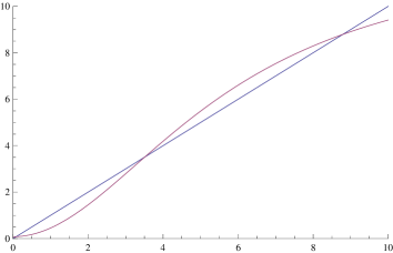
Figure 1. $Jp=34.6,J=-13.,T=27.5$

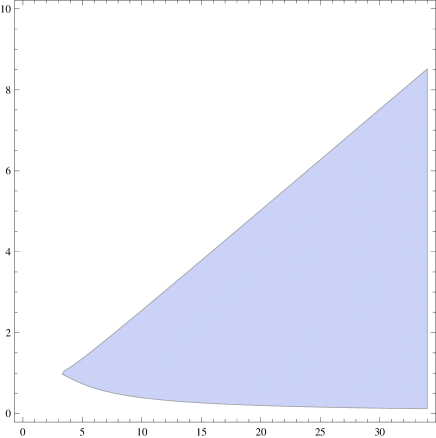
Figure 2. The region with three positive fixed points of the function (4)

5. Free energy

In this section, we study the free energy of depending on the boundary conditions for the Vannimenus Ising model on Cayley tree. By previous sections we know that for any boundary condition satisfying the equations (3.6) there exist Gibbs measures corresponding to the IV-model. For this model the partition function is given by

(5.1) $$Z_{n}=Z_{n}(\beta,h)=\sum\limits_{\sigma\in\Omega^{V_{n}}}\exp\big{\{}-\beta H_{n}(\sigma_{n})+\sum\limits_{x\in W_{n-1}}\sum\limits_{y\in S(x)}\sigma(x)\sigma(y)h_{xy,\sigma(x)\sigma(y)}\big{\}}.$$

Here the spin configurations $\sigma_{n}$ belong to $\Omega^{V_{n}}$ and

$$\textbf{h}=\{h_{xy,\sigma(x)\sigma(y)}\in\mathbb{R},x,y\in V\}$$

is a collection of real numbers that stands for boundary conditions. In this section we will investigate the dependence with respect to boundary conditions of the free energy defined as the limit:

(5.2) $$F(\beta,h)=\lim\limits_{n\to\infty}\frac{1}{\beta|V_{n}|}\ln Z_{n}(\beta,h).$$

Let us consider the equation

$$D(x,y)e^{\sigma(x)\sigma(y)h_{xy,\sigma(x)\sigma(y)}}=\prod\limits_{z\in S(y)}\sum\limits_{u\in\{\pm 1\}}e^{uh_{yz,\sigma(y)u}+\beta u(J\sigma(y)+J_{p}\sigma(x))}$$

$$U_{n-1}=\prod\limits_{x\in W_{n-2}}\prod\limits_{z\in S(y)}\sum\limits_{u\in\{\pm 1\}}D(x,y).$$

So, we have $Z_{n}=U_{n-1}Z_{n-1}.$

5.1. The free energies of translation-invariant Gibbs measures

In this section, we discuss the behavior of free energy as a function of the model in presence of an external field. We as before will consider the boundary conditions (4.1), i.e.

$$h_{xy,++}=h_{xy,-+}=h_{1}\mbox{ and }h_{xy,--}=h_{xy,+-}=h_{2}.\ \ \ \forall<x,y>\in L.$$

Proposition 5.1.

The free energies of compatible translation-invariant (TI) boundary condition exist and are given by

(5.3) $$F_{TI_{1}}(\beta,h) = -\frac{\ln 2}{\beta}-\ln\big{[}\cosh(h_{i}+\beta(J+J_{p}))\cosh(h_{i}+\beta(J-J_{p}))\big{]},$$

where $h_{i}$ are the varieties such that $u_{i}=e^{h_{i}}$ are the fixed points corresponding to the equations (3.6).

Proof.

From (4.1) one finds

(5.4) $$D(x,y)e^{h_{xy,++}} = \prod\limits_{z\in S(y)}\big{[}e^{h_{yz,++}+\beta(J+J_{p})}+e^{-h_{yz,+-}-\beta(J+J_{p})}\big{]}$$

$$= \prod\limits_{z\in S(y)}2e^{\frac{h_{yz,++}-h_{yz,+-}}{2}}\cosh\big{[}\frac{h_{yz,++}-h_{yz,+-}}{2}+\beta(J+J_{p})\big{]}.$$

(5.5) $$D(x,y)e^{-h_{xy,-+}} = \prod\limits_{z\in S(y)}\big{[}e^{h_{yz,++}+\beta(J-J_{p})}+e^{-h_{yz,+-}-\beta(J-J_{p})}\big{]}$$

$$= \prod\limits_{z\in S(y)}2e^{\frac{h_{yz,++}-h_{yz,+-}}{2}}\cosh\big{[}\frac{h_{yz,++}-h_{yz,+-}}{2}+\beta(J-J_{p})\big{]}.$$

Multiply the equations (5.4) and (5.5), then we have

(5.6) $$D(x,y) = 4\prod\limits_{z\in S(y)}b(y,z),$$

where

$$b(y,z)=e^{\frac{h_{yz,++}-h_{yz,+-}}{2}}\big{(}\cosh\big{[}\frac{h_{yz,++}-h_{yz,+-}}{2}+\beta(J+J_{p})\big{]}\cosh\big{[}\frac{h_{yz,++}-h_{yz,+-}}{2}+\beta(J-J_{p})\big{]}\big{)}^{\frac{1}{2}}.$$

$$U_{n-1} = \prod\limits_{x\in W_{n-2}}\prod\limits_{y\in S(x)}D(x,y)$$

$$= 4^{|W_{n-1}|}\prod\limits_{y\in W_{n-1}}\prod\limits_{z\in S(y)}b(x,y)=4^{|W_{n-1}|}e^{\sum\limits_{y\in W_{n-1}}\sum\limits_{z\in S(y)}\ln b(x,y)},$$

where $\mathfrak{a}(x,y)=\ln\mathfrak{b}(x,y).$
For this model, we can give the partition functions as follows;

$$Z_{n} = U_{n-1}Z_{n-1}$$

$$= 4^{|V_{n-1}|}e^{\sum\limits_{y\in W_{n-1}}\sum\limits_{z\in S(y)}\mathfrak{a}(y,z)}e^{\sum\limits_{y_{1}\in W_{n-2}}\sum\limits_{z_{1}\in S(y)}\mathfrak{a}(y_{1},z_{1})}\ldots e^{\sum\limits_{\widetilde{y}\in W_{0}}\sum\limits_{\widetilde{z}\in S(\widetilde{y})}\mathfrak{a}(\widetilde{y},\widetilde{z})}$$

$$= 4^{|V_{n-1}|}e^{\sum\limits_{<x,y>\in V_{n}}\mathfrak{a}(x,y)}.$$

Therefore, we get the free energy as follows;

(5.8) $$F_{TI_{1}}(\beta,h) = -\lim\limits_{n\to\infty}\frac{|V_{n-1}|}{\beta|V_{n}|}\ln D(x,y)$$

$$= -\frac{\ln 2}{\beta}-\ln\big{[}e^{h_{1}-h_{2}}\cosh(\frac{h_{1}+h_{2}}{2}+\beta(J+J_{p}))\cosh(\frac{h_{1}+h_{2}}{2}+\beta(J-J_{p}))\big{]}.$$

Assume that $e^{h_{1}}=e^{h_{1}}$. According to the formula (5.8), for the case 1 of Vannimenus Ising model the free energies of translation-invariant (TI) boundary condition are given by

(5.9) $$F_{TI_{1}}(\beta,h) = -\frac{\ln 2}{\beta}-\ln\big{[}\cosh(h_{i}+\beta(J+J_{p}))\cosh(h_{i}+\beta(J-J_{p}))\big{]},$$

where $h_{i}$ are the varieties such that $u_{i}=e^{h_{i}}$ are the fixed points corresponding to three cases. ∎

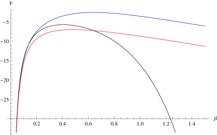
Figure 3. $J_{p}=34.6,J=-13,u_{1}=0.260261,u_{2}=1.18483,u_{3}=3.52491$

The residual entropy at $T=0$ is defined as follows:

(5.10) $$S_{\infty} = -\lim\limits_{\beta\to\infty}\frac{F(h)-F_{\infty}}{\frac{1}{\beta}},$$

where $F_{\infty}=\lim\limits_{\beta\to\infty}F(h).$

Let us compute the entropy

$$S(\beta,h) = -\frac{dF(\beta,h)}{dT}=\frac{dF(\beta,h)}{d\beta}\frac{1}{\beta^{2}}$$

$$= \frac{\ln 2}{\beta^{2}}-(J+J_{p})\tanh[h+\beta(J+J_{p})]-(J-J_{p})\tanh[h+\beta(J-J_{p})]$$

The residual entropy at $T=0$ is defined as follows:

(5.12) $$S_{\infty} = -\lim\limits_{\beta\to\infty}\frac{F(h)-F_{\infty}}{\frac{1}{\beta}},$$

where $F_{\infty}=\lim\limits_{\beta\to\infty}F(h).$

Let us compute the entropy

$$S(\beta,x_{i}) = -\frac{dF(\beta,h)}{dT}=\frac{dF(\beta,h)}{d\beta}\frac{1}{\beta^{2}}$$

$$= \frac{\ln 2}{\beta^{2}}-(J+J_{p})\tanh[\frac{\ln x_{i}}{2}+\beta(J+J_{p})]+(J+J_{p})\tanh[\frac{\ln x_{i}}{2}-\beta(J+J_{p})]$$

Acknowledgements The second named author (F.M.) thanks The Scientific and Technological Research Council of Turkey-TUBITAK for providing financial support and Zirve University for kind hospitality and providing all facilities.

References

- [1] H. Akın, U.A. Rozikov, S. Temir, A new set of limiting Gibbs measures for the Ising model on a Cayley tree. J. Stat. Phys. 142(2), 314-321 (2011).
- [2] P.M. Bleher, N.N. Ganikhodjaev, On pure phases of the Ising model on the Bethe lattice, Theor. Probab. Appl. 35, 216-227 (1990).
- [3] P.M. Bleher, J. Ruiz, V.A. Zagrebnov, On the purity of the limiting Gibbs state for the Ising model on the Bethe lattice, J. Stat. Phys. 79, 473-482 (1995).
- [4] Bak, P., Chaotic Behavior and Incommensurate Phases in the Anisotropic Ising Model with Competing Interactions, Phys.Rev. Lett. 46, 791-794 (1981)
- [5] Bak, P.: Commensurate phases, incommensurate phases and the devil’s staircase, Rep.Prog.Phys. 45, 587-629 (1982)
- [6] Bak, P. and J. von Boehm.: Ising model with solitons, phasons, and ”the devil’s staircase”, Phys.rev.B 21, 5297-5308 (1980)
- [7] Baxter, R.J.: Exactly Solved Models in Statistical Mechanics, Academic Press, London/ New York, (1982)
- [8] Bleher, P.M. and Ganikhodjaev, N.N.: On Pure Phases of the Ising Model on the Bethe Lattices, Theory Probab. Appl., 35, 216-227 (1990)
- [9] Bleher, P.M., Ruiz, J. and Zagrebvov, V.A.: On the purity of limiting Gibbs state for the Ising model on the Bethe lattice, J. Stat. Phys., 79, 473-482 (1995)
- [10] Dobrushin, R.L., Description of a random field by means of conditional probabilities and conditions of its regularity Theor. Prob. Appl., 13, 197-225 (1968)
- [11] Elliott, R.J.: Phenomenological Discussion of Magnetic Ordering in the Heavy Rare-Earth Metals, Phys. Rev 124, 346-353 (1961)
- [12] Fannes, M. and Verbeure, A.: On Solvable Models in Classical Lattice Systems, Commun. Math. Phys. 96, 115-124 (1984).
- [13] Fisher, M.E. and Selke, W.: Infinitely Many Commensurate Phases in a Simple Ising Model, Phys.Rev.Lett. 44, 1502-1505 (1980)
- [14] Ganikhodjaev, N.N.: Group representations and automorphisms of the Cayley tree, Dokl. Akad. Nauk. Rep. Uzbekistan 4, 3-5 (1994) (Russian)
- [15] Ganikhodjaev, N.N. and Rozikov, U.A.: Description of periodic extreme gibbs measures of some lattice models on the Cayley tree, Theor. Math. Phys., 111, 480-486 (1997).
- [16] Ganikhodjaev, N.N., Temir, S. and Akın, H.: Modulated Phase of a Potts Model with Competing Binary Interactions on a Cayley Tree, J. Stat. Phys., 137, 701-715 (2009).
- [17] Ganikhodjaev, N., Akın, H, Uguz, S., and Temir, S., Phase diagram and extreme Gibbs measures of the Ising model on a Cayley tree in the presence of competing binary and ternary interactions, Phase Transitions 84, no. 11-12, 1045 1063 (2011).
- [18] Ganikhodjaev, N., Akın, H, Uguz, S., and Temir, S., On extreme Gibbs measures of the Vannimenus model, J. Stat. Mech. Theor. Exp. 2011, no. 03 (2011): P03025.
- [19] D. Gandolfo, J. Ruiz, and S. Shlosman, A manifold of pure Gibbs states of the Ising model on a Cayley tree, J. Stat. Phys. 148 999-1005 (2012).
- [20] D. Gandolfo, M. M. Rakhmatullaev, U. A. Rozikov, J. Ruiz, On free energies of the Ising model on the Cayley tree, J. Stat. Phys. 150 (6), 1201-1217 (2013).
- [21] D. Gandolfo, F. H. Haydarov, U. A. Rozikov, J. Ruiz, New phase transitions of the Ising model on Cayley trees, J. Stat. Phys. 153 (3), 400-411 (2013).
- [22] N.N. Ganikhodjaev, U.A. Rozikov, A description of periodic extremal Gibbs measures of some lattice models on the Cayley tree, Theor. Math. Phys. 111 480-486 (1997).
- [23] Georgii, H.-O.: Gibbs Measures and Phase Transitions (de Gruyter Stud. Math., Vol.9), Walter de Gruyter, Berlin, New York (1988)
- [24] Inawashiro, S., Thompson, C.J.: Competing Ising Interactions and Chaotic Glass-Like Behaviour on a Cayley Tree, Physics Letters , 97A, 245-248 (1983).
- [25] Ioffe, D.: A note on the extremality of the disordered state for the Ising model on the Bethe lattice Lett. Math. Phys., 37, 137-143 (1996).
- [26] M.H. Jensen and P. Bak.: Mean-field theory of the three-dimensional anisotropic Ising model as a four-dimensional mapping, Phys. Rev. B 27, 6853-6868 (1983)
- [27] S. Katsura, M. Takizawa.: Bethe lattice and the Bethe approximation. Prog. Theor. Phys. 51, 82-98 (1974).
- [28] S. H. Kung, Sums of Integer Powers via the Stolz-Cesaro Theorem, Math. Assoc. America. 40: 42-44 (2009).
- [29] Lanford, O.E., and Ruelle, D.: Observables at infinity and states with short range correlations in statistical mechanics. Communications in Mathematical Physics, 13 (3), 194-215 (1969).
- [30] Mariz,M., Tsallis,C., Albuquerque, A.L.: Phase Diagram of the Ising Model on a Cayley tree in the Presence of competing Interactions and Magnetic Field, Jour. Stat. Phys. 40, 577-592 (1985).
- [31] Newman, M.E.J.: Phys. Rev. Lett. 103, 058701 (2009).
- [32] F. Mukhamedov, M. Dogan and H. Akın, Phase transition for the p-adic Ising Vannimenus model on the Cayley tree, J. Stat. Mech. Theor. Exp., (2014) P10031, pp. 1-21.
- [33] Preston, Ch.J.: Gibbs States on Countable Sets, Cambridge Univ.Press, Cambridge (1974).
- [34] Rozikov, U., Gibbs Measures on Cayley Trees, World Scientific Publishing Company (2013).
- [35] Rozikov, U., Gibbs measures on cayley trees: Results and open problems, Reviews in Mathematical Physics 25, no. 01. (2013).
- [36] U.A. Rozikov, M.M. Rakhmatullaev, On weakly periodic Gibbs measures of the Ising model on a Cayley tree., Theor. Math. Phys. 156(2): 1218-1227 (2008).
- [37] U.A. Rozikov, M.M. Rakhmatullaev, Weakly periodic ground states and Gibbs measures for the Ising model with competing interactions on the Cayley tree, Theor. Math. Phys. 160: 1291-1299 (2009).
- [38] Tragtenberg, M.H.R., Yokoi, C.S.O.: Field Behaviour of an Ising Model with Competing Interactions on the Bethe Lattice, Phys. Rev. E, 52, 2187-2197 (1995).
- [39] Vannimenus, J.: Modulated phase of an Ising system with competing interactions on a Cayley tree, Zeitschrift fur Physik B Condensed Matter, 43 no. 2, 141 148 (1981).
- [40] Yokoi, C.S.O., Oliveira, M.J., Salinas, S.R., Strange Attractor in the Ising Model with Competing Interactions on the Cayley Tree, Phys. Rev. Lett., 54, 163-166 (1985).
- [41] S. Zachary, Countable state space Markov random Felds and Markov chains on trees. Ann. Prob. 11, 894-903 (1983).