Networks Systems obeying scaling laws

Analytical results for the distribution of shortest path lengths in random networks

Abstract

We present two complementary analytical approaches for calculating the distribution of shortest path lengths in Erdős-Rényi networks, based on recursion equations for the shells around a reference node and for the paths originating from it. The results are in agreement with numerical simulations for a broad range of network sizes and connectivities. The average and standard deviation of the distribution are also obtained. In the case that the mean degree scales as $N^{\alpha}$ with the network size, the distribution becomes extremely narrow in the asymptotic limit, namely almost all pairs of nodes are equidistant, at distance $d=\lfloor 1/\alpha\rfloor$ from each other. The distribution of shortest path lengths between nodes of degree $m$ and the rest of the network is calculated. Its average is shown to be a monotonically decreasing function of $m$, providing an interesting relation between a local property and a global property of the network. The methodology presented here can be applied to more general classes of networks.

The increasing interest in network research in recent years is motivated by the realization that a large variety of systems and processes which involve interacting objects can be described by network models [1, 2, 3, 4]. In these models, the objects are represented by nodes and the interactions are expressed by edges. Pairs of connected nodes can affect each other directly. However, the interactions between most pairs of nodes are indirect, mediated by intermediate nodes and edges. Important properties of these indirect interactions such as their strengths, delay times, coordination, correlation and synchronization depend on the paths between different nodes. A pair of nodes, $i$ and $j$, may be connected by a large number of paths. The shortest among these paths are of particular importance because they are likely to provide the fastest and strongest interaction between these two nodes. Therefore, it is of interest to study the distribution of shortest path lengths (DSPL) between nodes in different types of networks. Such distributions are expected to depend on the network structure and size.

Random networks of the Erdős-Rényi (ER) type were studied extensively since the 1950’s [5, 6, 7] using mathematical methods and computer simulations [8]. The increasing availability of empirical data on networks since the late 1990’s stimulated much theoretical interest, leading to new results for ER networks [9, 10]. Measures such as the diameter and the average path length were studied extensively [11, 12]. However, apart from a few studies, the entire DSPL has attracted little attention [13, 14, 15]. This distribution is of great importance for the temporal evolution of dynamical processes on networks, such as signal propagation, navigation and epidemic spreading [16]. It determines the number of nodes exposed to a propagating signal originated from a given node as a function of time. More generally, the shortest paths can be considered as the backbone of a more complete set of paths between pairs of nodes. While the shortest paths provide the fastest propagation, signals also utilize longer paths which are more numerous. This was demonstrated in studies of first passage times in diffusive processes on networks [17].

In this Letter we present two analytical approaches for calculating the DSPL between nodes in the ER network, referred to as the recursive shells approach (RSA) and the recursive paths approach (RPA). Using recursion equations we study this distribution in different regimes, namely sparse and dense networks of small as well as asymptotically large sizes. Consider an ER network of $N$ nodes, where each pair of nodes is independently connected with probability $p$. We denote such a network by ER($N,p$). Its degree sequence follows the Poisson distribution with the parameter $Np$, which is equal to the average degree. Such networks are often studied in the asymptotic limit, where $N\rightarrow\infty$. In this limit, one can identify different regimes, according to the scaling of $p$ vs. $N$.

For sparse networks, denoted by ER($N,c/N$), the average degree is $c=Np$. At $c=1$ there is a percolation transition. For $c<1$, the network consists of small isolated clusters. For $c>1$, a giant component of size which scales linearly with $N$ is formed, in addition to the small, isolated components of maximal size which scales as $\ln N$ [8]. For dense networks, the parameter $p$ scales as $N^{\alpha-1}$, where $0<\alpha<1$, the mean connectivity grows with the network size as $N^{\alpha}$ and the number of isolated components vanishes.

When a pair of nodes resides on the same connected sub-network, one can identify paths connecting these nodes. The path length is the number of edges along the path. The distance $d_{ij}$ between a pair of different nodes $i$ and $j$ is the length of the shortest path connecting them. When $i$ and $j$ reside on different sub-networks, there is no path between them and thus $d_{ij}\equiv\infty$. The tail-distribution $F_{N}(k)=Pr(d>k)$, $k=0,1,2,\dots,N-1$, is the probability that the distance $d$ between a random pair of nodes in an ER network of size $N$ is larger than $k$. Clearly, the probability that two distinct random nodes are at a distance $d>0$ from each other is $F_{N}(0)=1$, while the probability that $d>1$, namely they are not directly connected, is $F_{N}(1)=q$, where $q=1-p$. The probability distribution $P_{N}(k)$ can be recovered as $P_{N}(k)=F_{N}(k-1)-F_{N}(k)$, $k=1,2,\dots,N-1$. The probability $F_{N}(k)$ does not necessarily converge to zero in the limit $k\rightarrow\infty$. Its asymptotic value $F(\infty)$ is equal to the fraction of pairs of nodes in the network which belong to different clusters, namely for which $d_{ij}=\infty$. In fact, $F(\infty)$ can be estimated independently by using known properties of the fraction of nodes, $g$, which belongs to the giant component in the asymptotic limit [8]. This fraction satisfies $g=1-\exp(-cg)$ and $F(\infty)=1-g^{2}$. In a finite network $F(\infty)$ can be replaced by $F_{N}(N-1)$ since the longest possible distance is $d=N-1$.

In the RSA, one picks a random node, $i$, as a reference node and examines the shell structure of the rest of the network around it. The number of nodes which are at a distance $d>k$, $k=0,1,2,\dots,N-1$, from the reference node is denoted by $\overline{N}_{k}$. The number of nodes at distance $d=k$ from the reference node is denoted by $N_{k}$, where $N_{0}=1$ and $N_{k}=\overline{N}_{k-1}-\overline{N}_{k}$ for $k\geq 1$. The $N_{k}$’s obey the recursion equation $N_{k+1}=\overline{N}_{k}(1-q^{N_{k}})$, which can be re-written as a second order difference equation of the form $\overline{N}_{k+1}=\overline{N}_{k}q^{\overline{N}_{k-1}-\overline{N}_{k}}$, where $\overline{N}_{0}=N-1$ and $\overline{N}_{1}=(N-1)q$. Using the relation $\overline{N}_{k}=(N-1)\cdot F_{N}(k)$, it can be expressed as

$$F_{N}(k+1)=F_{N}(k)q^{(N-1)[F_{N}(k-1)-F_{N}(k)]},$$ (1)

where $F_{N}(0)=1$ and $F_{N}(1)=q$.

In the RPA one first picks two distinct random nodes, $i$ and $j$. The probability that the distance between them is larger than $k$ can be related to the probability that it is larger than $k-1$ by $F_{N}(k)=F_{N}(k-1)P_{N}(d>k|d>k-1)$, where $P_{N}(d>k|d>k-1)$ is the conditional probability that the distance is larger than $k$, given that it is larger than $k-1$. The iteration of this relation yields

$$F_{N}(k)=F_{N}(1)\prod_{m=2}^{k}P_{N}(d>m|d>m-1).$$ (2)

This means that in order to obtain the distribution $F_{N}(k)$, all we need to calculate are the conditional probabilities $P_{N}(d>m|d>m-1)$, for all values of $2\leq m\leq k$.

Consider a path of length $k$ starting at node $i$ and ending at node $j$ (assuming that there is no such path of length $k-1$ or less). The path can be decomposed into a single edge from node $i$ to an intermediate node $\ell$ and a shorter path of length $k-1$ from $\ell$ to $j$. Such a path can be ruled out in two ways: either there is no edge between $i$ and $\ell$ (with probability $q$), or, in case that there is such an edge - there is no path of length $k-1$ between $\ell$ and $j$. The probability of the latter is $P_{N-1}(d>k-1|d>k-2)$, since the remaining path is embedded in a smaller network of $N-1$ nodes. Combining the two possibilities yields the recursion equation

$$P_{N}(d>k|d>k-1)=\left[q+p\cdot P_{N-1}(d>k-1|d>k-2)\right]^{N-2},$$ (3)

where the right hand side is raised to the power $N-2$ in order to account for all possible ways to choose the intermediate node $\ell$. In Fig. 1 we present the possible paths of length $k$ between $i$ and $j$. This approach follows the spirit of the renormalization group theory [18], since the removal of a node from the network reduces the size of the configuration space by a factor of $2^{N-1}$. This process is repeated $k-1$ times, reducing the network down to size $N^{\prime}=N-k+1$ and closing the recursion equations with $P_{N^{\prime}}(d>1|d>0)=F_{N^{\prime}}(1)=q$.

[width=10cm]fig1.eps

Figure 1: (Color online) Illustration of the possible paths of length $k$ between two random nodes $i$ and $j$ in an ER network of $N$ nodes. The first edge of such path connects node $i$ to some other node $\ell$, which may be any one of the remaining $N-2$ nodes. The rest of the path, from $\ell$ to $j$ is of length $k-1$ and it resides on a smaller network of $N-1$ nodes. The path of length $k$ from $i$ to $j$ exists only when both the edge from $i$ to $\ell$ and the path of length $k-1$ from $\ell$ to $j$ exist.

Interestingly, inserting $k=2$ in Eq. (3) gives rise to the simple and exact expression

$$P_{N}(d>2|d>1)=(1-p^{2})^{N-2}.$$ (4)

Each path of length $k=2$ between nodes $i$ and $j$ consists of a single intermediate node and two edges. These paths do not overlap and are thus independent. Paths of lengths $k>2$ may share edges with other paths of the same length as well as with shorter paths. Therefore, in the calculation of the DSPL we use conditional probabilities to ensure that no shorter paths exist. This approach eliminates the correlations between paths of different lengths. On the other hand, nodes $i$ and $j$ may be connected by several paths of the same length, which may share some edges and thus become correlated. The RPA does not account for such correlations, because it assumes that the sub-networks of size $N-1$ are independent. Averaging over the quenched randomness in each instance of such network, the RPA provides the distribution over an ensemble of networks.

In the limit $p\rightarrow 0$ one can simplify the recursion equations and obtain the approximate closed form expression

$$P_{N}(d>k|d>k-1)=(1-p^{k})^{(N-2)\dots(N-k)},$$ (5)

for any value of $k$. This expression is obtained using induction, based on Eq. (3) and the exact result given above for $k=2$. This can be understood intuitively since the total number of possible paths of length $k$ between nodes $i$ and $j$ is given by the product ${(N-2)\dots(N-k)}$, and the probability for each of these paths to be connected is given by $p^{k}$. This approximation breaks down for values of $p$ which are not exceedingly small, where the correlations between different paths build up and cannot be ignored.

The regime of sparse networks was studied extensively, focusing on the diameter (namely, the largest distance between any pair of nodes) of the giant cluster, which scales like a constant times $\ln N$, where the constant is $1/\ln c-2/\ln c^{\prime}$, where $c^{\prime}<1$ satisfies the equation $c^{\prime}\exp(-c^{\prime})=c\exp(-c)$ [19]. In the strongly connected regime, we focus on the case in which $p=bN^{\alpha-1}$, where $b>0$ and $0<\alpha<1$. In this case the average degree increases with the network size as $N^{\alpha}$. We will now derive an asymptotic result for the limit $N\rightarrow\infty$. In this limit $p\rightarrow 0$ and therefore the simplified results of Eq. (5) can be used. Plugging the scaling of $p$ vs. $N$ into Eq. (5) one obtains

$$P_{N}(d>k|d>k-1)\simeq\left(1-\frac{b^{k}}{N^{k(1-\alpha)}}\right)^{N^{k-1}}.$$ (6)

For $N\rightarrow\infty$, $P_{N}(d>k|d>k-1)\rightarrow P(d>k|d>k-1)$, where $P(d>k|d>k-1)=1$ for $k<1/\alpha$, $\exp{(-b^{1/\alpha})}$ for $k=1/\alpha$ and $0$ for $k>1/\alpha$. Note that the second case in the above equation is obtained only in the special case of $\alpha=1/r$, where $r$ is an integer. Therefore, we will first consider the generic case in which $\alpha$ is not an exact inverse of an integer. Inserting the result for the conditional probabilities into Eq. (2) we obtain

$$P(k)=\left\{\begin{array}[]{lr}1&:k=\lfloor\frac{1}{\alpha}\rfloor+1\\ 0&:{\rm otherwise},\end{array}\right.$$ (7)

where $\lfloor x\rfloor$ is the integer part of $x$. In case that $\alpha=1/r$ we obtain that

$$P(k)=\left\{\begin{array}[]{lr}1-e^{-b^{r}}&:k=r\\ e^{-b^{r}}&:k=r+1\\ 0&:{\rm otherwise}.\end{array}\right.$$ (8)

These results can be understood intuitively using the following argument. Starting from node $i$, we define the shell of radius $d=1$ around it as the set of nodes which are directly connected to $i$. The expected value for the number of nodes in this shell is $N_{1}\sim N^{\alpha}$. Proceeding by induction, the shell of radius $d$ is denoted as the set of nodes which are directly connected to nodes in the shell of radius $d-1$. Thus, the number of nodes in the shell of radius $d$ is given by $N_{d}\sim N^{d\alpha}$. In the asymptotic limit, as long as $d\alpha<1$, the shell of radius $d$ still consists of an exceedingly small fraction of the nodes in the network. On the other hand, once $d\alpha>1$, this shell includes almost every node in the network. This means that almost all the nodes in the network are at a distance $d=\lfloor 1/\alpha\rfloor+1$ from node $i$. Since node $i$ was chosen at random, this means that the shortest path between almost any pair of nodes in the network is of length $d$.

The case of $\alpha=1/r$, where $r$ is an integer, requires a special consideration. Based on the argument presented above, the neighborhood of radius $d=r$ from node $i$ should include all the $N$ nodes. However, this counting includes duplications, namely nodes which are connected to node $i$ by several paths of length $r$. As a result, there are other nodes which are not reached by any of these paths. Since the number of nodes of distance $r$ from node $i$ scales with $N$, it is clear that each one of the remaining nodes is connected to at least one of them. Therefore, the remaining nodes are at a distance $d=r+1$ from node $i$.

Before presenting the results obtained from the two approaches, we refer to an earlier study of the DSPL in ER networks [13]. We briefly summarize their approach, adapting the notation where appropriate. The expectation value for the number of nodes at a distance $k-1$ or less from the reference node is given by: $n(k)=[1-F_{N}(k-1)]N$. This is due to the fact that the probability for a random node to be at a distance smaller than $k$ is $(1-F_{N}(k-1))$, and multiplying by $N$ one obtains $n(k)$. In order for a node to be at a distance larger than $k$ from the reference node, it must not be directly connected to any of the $n(k)$ nodes which are at distance $k-1$ or less from the reference node. Picking a random node, the probability that it will not be connected to any of these nodes is given by [13]

$$F_{N}(k)=q^{[1-F_{N}(k-1)]N}.$$ (9)

This recursion equation can be iterated, starting from $F_{N}(0)=(N-1)/N$, to obtain $F_{N}(k)$ for $k=1,2,...$. A potential problem with this approach is that in the estimation of the probability, $F_{N}(k)$, that a random node will be at distance larger than $k$ from the reference node, Eq. (9) ignores the possibility that the random node is already connected to the reference node by a path of length $k-1$ or less. This is expected to bias the distribution towards larger distances.

In Fig. 2 we present the tail distribution $F_{N}(k)$ vs. $k$, for an ER network of $N=1000$ nodes and $p=c/N$, where $c=2.5$, obtained from numerical simulations for all pairs of nodes ($\times$) and for pairs of nodes on the same cluster ($+$). We also present the theoretical results obtained from the RSA ($\square$). and from the RPA ($\circ$). The results of the RSA agree well with the numerical results for all pairs, except for the limit of large distances where the plateau in $F_{N}(k)$ is lower than the empirical curve. It means that this approach underestimates the fraction of pairs for which $d_{ij}=\infty$, which is equal to $F(\infty)$. The results of the RPA agree well with the numerical results for pairs which reside on the same cluster. This is due to the fact that this approach reconstructs the remaining network at each iteration of the recursion equations. As a result, the quenched randomness of the connectivities in each realization of the network is annealed, eliminating the isolated nodes and the small, isolated clusters. In the RSA there is no such annealing. Therefore, the RSA applies to all pairs of nodes in the network while the RPA applies to pairs of nodes on the same cluster. In the limit of dense networks there are no isolated components and the two approaches coincide.

[width=10cm]fig2.eps

Figure 2: (Color online) (a) The tail distribution $F_{N}(k)$, vs. $k$ for the ER($N,c/N$) network with $N=1000$ and $c=2.5$, obtained from numerical simulations for all pairs of nodes ($\times$) and for pairs of nodes on the same cluster ($+$). The results of the RSA ($\square$) agree well with the numerical results for all pairs of nodes, except for the asymptotic tail. The results of the RPA ($\circ$) agree well with the numerical results for pairs of nodes on the same cluster.

The distribution $P_{N}(k)$ can be characterized by its moments. The $n$th moment, $\langle k^{n}\rangle$, can be obtained using the tail-sum formula $\langle k^{n}\rangle=\sum_{k=0}^{N-1}[(k+1)^{n}-k^{n}]F_{N}(k)$. In particular, the first moment is given by $\langle k\rangle=\sum_{k=0}^{N-1}F_{N}(k)$ and the second moment by $\langle k^{2}\rangle=\sum_{k=0}^{N-1}(2k+1)F_{N}(k)$. The width of the distribution can be characterized by the variance $\sigma^{2}=\langle k^{2}\rangle-\langle k\rangle^{2}$. Related topological indices [20] such as the Wiener index [21] and the Harary index [22, 23, 24] were studied in the context of chemical graphs. It was shown that important properties of molecules can be obtained using such indices for the graphs representing their structure [21].

,         ,

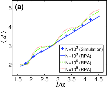
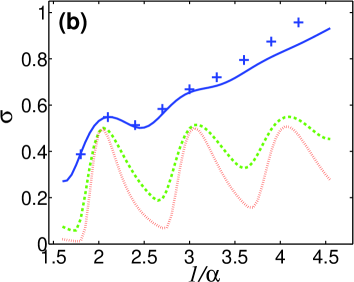
Figure 3: (Color online) The average $\langle d\rangle$ (a) and the standard deviation $\sigma$ (b) of the DSPL in the ER($N,bN^{\alpha-1}$) network vs. $1/\alpha$ for $b=1$ and $N=10^{3}$ (solid line) $10^{6}$ (dashed line) and $10^{9}$ (dotted line), obtained from the RPA. It is observed that $\langle d\rangle\simeq\lfloor 1/\alpha\rfloor+1$, decorated by a rounded step function, while $\sigma$ exhibits oscillations with maxima at integer values of $1/\alpha$.

In Fig. 3(a) we present the average distance $\langle d\rangle$ between pairs of nodes vs. $1/\alpha$ in dense ER networks. Following Eqs. (7)-(8), these functions converge to a staircase form as $N\rightarrow\infty$. In Fig. 3(b) we present the standard deviation $\sigma$ vs. $1/\alpha$. For finite networks it exhibits oscillations of unit period. In the asymptotic limit the peaks become vanishingly narrow around the integers.

So far we have studied the DSPL between all pairs of nodes in the network. Below, we consider a reference node $i$ of a known degree, $m$, and study the DSPL between this node and the rest of the network. We denote the DSPL between a random node $i$ of degree $m$ and other random nodes, $j$, by $F_{N|m}(k)=F_{N}(k|deg(i)=m)$ and the corresponding conditional probability by $P_{N|m}(d>k|d>k-1)$. In this case, the first iteration of the recursion equation takes the form

$$P_{N|m}(d>k|d>k-1)=[P_{N-1}(d>k-1|d>k-2)]^{m},$$ (10)

where the expression on the right hand side is obtained from Eq. (3). In Fig. 4 we present the tail distribution $F_{N|m}(k)$ vs. $k$, obtained from numerical simulations for $m=1$ (+), $3$ ($\times$) and $7$ ($\ast$), in a dilute ER network of $N=1000$ and $c=2.5$. Each data point is averaged over $20$ independent realizations of the network. The results of the RPA for $m=1$ ($\diamond$), $3$ ($\square$) and $7$ ($\circ$) are in good agreement with the numerical results. Clearly, the distribution is strongly affected by the local connectivity of the reference node. The knee of the distribution $F_{N|m}(k)$ (which coincides with the peak of the corresponding probability density function) moves to the left as $m$ is increased. This means that nodes which are strongly connected at the local level are closer to the rest of the network than weakly connected nodes.

[width=12cm]fig4.eps

Figure 4: (Color online) The DSPL $F_{N|m}(k)$ vs. $k$ between a random node $i$ of a given degree, $m$, and all other nodes which reside on the same cluster in a dilute ER network of $N=1000$ and $c=2.5$. The results of the RPA for $m=1$ ($\diamond$), $3$ ($\square$) and $7$ ($\circ$) are in good agreement with the corresponding numerical results: $m=1$ (+), $3$ ($\times$) and $7$ ($\ast$).

In summary, we have studied the distribution of shortest path lengths in ER networks using two complementary theoretical approaches and showed that they are in good agreement with numerical results. For large and dense networks the distribution becomes extremely narrow and is exactly captured by both approaches. A slight modification enables us to calculate the DSPL around a node with a given degree, $m$. The results exemplify the impact of local features (such as the degree of a node) on global properties (such as the distance distribution) in complex networks. The proposed theoretical approaches are highly flexible and can be applied to more general networks [25, 26].

- [1] \NameAlbert R. Barabási A. L. \REVIEWRev. Mod. Phys.74200247.
- [2] \NameCaldarelli G. \BookScale free networks: complex webs in nature and technology \PublOxford University Press, Oxford \Year2007.
- [3] \NameNewman M.E.J. \BookNetworks: an Introduction \PublOxford University Press, Oxford \Year2010.
- [4] \NameEstrada E. \BookThe structure of complex networks: Theory and applications \PublOxford University Press, Oxford \Year2011.
- [5] \NameErdős P.Rényi A. \REVIEWPubl. Math.61959290.
- [6] \NameErdős P.Rényi A. \REVIEWPubl. Math. Inst. Hung. Acad. Sci.5196017.
- [7] \NameErdős P.Rényi A. \REVIEWBull. Inst. Int. Stat.381961343.
- [8] \NameBollobás B. \BookRandom Graphs \PublCambridge University Press, Cambridge \Year2001.
- [9] \Namevan der Hofstad R., Hooghiemstra G. Van Mieghem P. \REVIEWRandom Structures and Algorithms27200576.
- [10] \NameDe Bacco C., Majumdar S. N. Sollich P. \REVIEWJ. Phys. A: Math. Theor.482015205004.
- [11] \NameWatts D. J. Strogatz S. H. \REVIEWNature3931998440.
- [12] \NameFronczak A., Fronczak P. Holyst J. A. \REVIEWPhys. Rev. E702004056110.
- [13] \NameBlondel V. D., Guillaume J.-L., Hendrickx J. M. Jungers R. M. \REVIEWPhys. Rev. E762007066101.
- [14] \NameDorogotsev S. N., Mendes J. F. F. Samukhin A. N. \REVIEWNuclear Physics B6532003307.
- [15] \Namevan der Esker H., van der Hofstad R. Hooghiemstra G. \REVIEWJ. Stat. Phys.1332008169.
- [16] \NamePastor-Satorras R. Vespignani A. \REVIEWPhys. Rev. Lett.8620013200.
- [17] \NameSood V., Redner S. ben-Avraham D. \REVIEWJ. Phys. A382005109.
- [18] \NameBinney J. J., Dowrick N. J., Fisher A. J. Newman M. E. J. \BookThe Theory of Critical Phenomena \PublClarendon Press, Oxford \Year1993.
- [19] \NameRiordan O. Wormald N. \REVIEWCombinatorics, Probability, and Computing192010835.
- [20] \NameDehmer M. Emmert-Streib F. \BookQuantitative Graph Theory \PublChapman and Hall/CRC, Boca Raton, FL, USA \Year2014.
- [21] \NameWiener H. \REVIEWJ. American Chem. Soc.69194717.
- [22] \NameMihalić Z. Trinajsti N. \REVIEWJournal of Chemical Education691992701.
- [23] \NameIvanciuc O., Balaban T. S. Balaban A. T. \REVIEWJ. Math. Chem.121993309.
- [24] \NamePlavs̆ić D., Nikolić S., Trinajsti N. Mihalić Z. \REVIEWJ. Math. Chem.121993235.
- [25] \NameCaldarelli G., Capocci A., De Los Rios P. Muñoz M. A. \REVIEWPhys. Rev. Lett.892002258702.
- [26] \NameBoguñá M. Pastor-Satorras R. \REVIEWPhys. Rev. E682003036112.