Rapidly computable viscous friction and no-slip
rigid contact models

Abstract

This article presents computationally efficient algorithms for modeling two special cases of rigid contact—contact with only viscous friction and contact without slip—that have particularly useful applications in robotic locomotion and grasping. Modeling rigid contact with Coulomb friction generally exhibits $O(n^{3})$ expected time complexity in the number of contact points and $2^{O(n)}$ worst-case complexity. The special cases we consider exhibit $O(m^{3}+m^{2}n)$ time complexity ($m$ is the number of independent coordinates in the multi rigid body system) in the expected case and polynomial complexity in the worst case; thus, asymptotic complexity is no longer driven by number of contact points (which is conceivably limitless) but instead is more dependent on the number of bodies in the system (which is often fixed). These special cases also require considerably fewer constrained nonlinear optimization variables thus yielding substantial improvements in running time. Finally, these special cases also afford one other advantage: the nonlinear optimization problems are numerically easier to solve.

I Introduction

Dynamic robotic simulation; grasp planning; and, increasingly, locomotion planning and control employ rigid contact models with dry (typically Coulomb) and wet (viscous) friction. These contact models yield an effective tradeoff between computation speed and physical accuracy. While rigid contact models are far faster than, e.g., elastodynamic finite element analysis, they still require heavy computation: the expected time complexity for such models is $O(n^{3})$ in the number of contact points. Additionally, the number of contact points input to the model is conceivably limitless. This issue is not just theoretically interesting: Wang [25] reports that solving the contact problem absorbs up to 90% of computation time when simulating a scenario for the DARPA Robotics Challenge using ODE [19].

Roboticists are often content to use rigid contact models without Coulomb friction for computational expediency. For example, one may wish to model locomotion or effect simulated grasping without observing slip; roboticists studying legged locomotion often predicate their models on no slip occurring, for example. If slip is desirable, purely viscous friction might yield a suitable model if, for example, a robot is walking on a wet surface. This article presents computationally efficient methods for both of these special cases.

These special cases provide the following computational and modeling advantages: (1)​ time complexity goes from worst-case exponential (the worst-case complexity of solving rigid contact problems with Coulomb friction [23, 1] using Lemke’s Algorithm [15]) to worst-case polynomial in the number of contact points; (2)​ significant reduction in the number of nonlinear optimization problem variables; and (3)​ a positive-semi-definite-matrix linear complementarity problem (LCP), in place of a copositive-plus LCP, which is demonstrably easier to solve [8] (i.e., the solver is less likely to fail due to numerical errors) and permits the use of general algorithms for solving convex optimization problems.

Finally, we provide an algorithm that yields $O(m^{3}+m^{2}n)$ expected asymptotic time complexity on these two contact models, where $m$ is the number of independent coordinates in the multi rigid body system. This algorithm therefore provides a means to make complexity more dependent on the number of independent coordinates in the system (this number remains constant except in the unusual case in which bodies are inserted into the simulation) than on the number of contact points (which is conceivably unlimited).

II LCPs, NCPs, and MLCPs

A LCP, or linear complementarity problem, ($\bm{r},\mathbf{Q}$) signifies the problem:

$$\bm{w} =\mathbf{Q}\bm{z}+\bm{r}$$

$$\bm{w} \geq\bm{0}$$

$$\bm{z} \geq\bm{0}$$

$${\bm{z}}^{\mathsf{T}}\bm{w} =0$$

for unknown vectors $\bm{z},\bm{w}\in\mathbb{R}^{q}$.

A nonlinear complementarity problem (NCP) is composed of a number of nonlinear complementarity constraints [6] that take the form:

$$\bm{x} \geq\bm{0}$$ (1)

$$f(\bm{x}) \geq\bm{0}$$ (2)

$${\bm{x}}^{\mathsf{T}}f(\bm{x}) =0$$ (3)

where $\bm{x}\in\mathbb{R}^{q}$ and $f:\mathbb{R}^{q}\to\mathbb{R}^{q}$.

A mixed linear complementarity problem (MLCP) is defined by the following constraints:

$$\mathbf{A}\bm{x}+\mathbf{C}\bm{y}+\bm{g} =\bm{0}$$ (4)

$$\mathbf{D}\bm{x}+\mathbf{B}\bm{y}+\bm{h} \geq\bm{0}$$ (5)

$$\bm{y} \geq\bm{0}$$ (6)

$${\bm{y}}^{\mathsf{T}}(\mathbf{C}\bm{x}+\mathbf{D}\bm{y}+\bm{h}) =0$$ (7)

Note that the $\bm{x}$ variables are unconstrained, while the $\bm{y}$ variables must be non-negative. If $\mathbf{A}$ is non-singular, the unconstrained variables can be computed as:

$$\bm{x}=-{\mathbf{A}}^{\mathsf{-1}}(\mathbf{C}\bm{y}+\bm{g})$$ (8)

Substituting $\bm{x}$ into equations 4–7 yields the LCP ($\bm{e},\mathbf{F}$):

$$\mathbf{F} \equiv\mathbf{B}-\mathbf{D}{\mathbf{A}}^{\mathsf{-1}}\mathbf{C}$$ (9)

$$\bm{e} \equiv\bm{h}-\mathbf{D}{\mathbf{A}}^{\mathsf{-1}}\bm{g}$$ (10)

A solution $(\bm{y},\bm{\nu})$ to this LCP obeys the relationship $\mathbf{F}\bm{y}+\bm{e}=\bm{\nu}$; once one has $\bm{y}$, $\bm{x}$ may be determined via Equation 8, and the MCLP is solved.

III Background

III-A Coulomb friction

Coulomb’s friction model provides relationships between the force applied along the contact normal and the frictional forces. Coulomb friction considers two cases, rolling/sticking and sliding. The former occurs when the velocity is zero in the tangent plane of the contact frame; conversely, sliding occurs when that velocity is non-zero.

The magnitude of the friction force for a sliding contact modeled with Coulomb friction is given by the equation:

$$f_{f}=\mu_{c}f_{n}$$ (11)

where $f_{n}$ is the magnitude of the force applied along the contact normal. The frictional force is applied directly opposite the direction of sliding (i.e., against the relative velocity in the tangent plane of the contact frame).

The magnitude of the friction force for a rolling or sticking contact modeled with Coulomb friction is given by the equation:

$$f_{f}\leq\mu_{c}f_{n}$$ (12)

In the case of rolling/sticking friction, the friction force acts to resist motion in the tangent (e.g., in the case of a box resting on a slope); thus, $f_{f}$ may be strictly less than $\mu_{c}f_{n}$. If external forces become sufficiently large to overcome rolling/sticking friction forces, the rolling/sticking contact will transition to sliding.

Many applications in robotics use the Coulomb friction model because it is relatively straightforward to compute—one can determine the frictional forces without integrating ordinary differential equations—and it is reasonably predictive. Nevertheless, Coulomb friction is somewhat expensive (computationally) to model: the rigid contact models of Stewart and Trinkle [23] and Anitescu and Potra [1] can be solved in expected polynomial time in the $n$ contacts, though exponential complexity may be exhibited in the worst case.

III-B Acceleration-level rigid body contact model with Coulomb and viscous friction

We now describe the rigid contact model with Coulomb and viscous friction that uses only non-impulsive forces for consistency with the principle of constraints [10]. The multi rigid body dynamics equation with contact and joint constraint forces is given below:

$$\mathbf{M}(t)\dot{\bm{v}}= \bm{f}(t)+{\mathbf{J}(t)}^{\mathsf{T}}\bm{f}_{j}+{\mathbf{N}(t)}^{\mathsf{T}}\bm{f}_{n}+\ldots$$ (13)

$${\mathbf{S}_{k}(t)}^{\mathsf{T}}\bm{f}_{s}+{\mathbf{T}_{k}(t)}^{\mathsf{T}}\bm{f}_{t}-{\mathbf{Q}(t)}^{\mathsf{T}}\bm{f}_{q}-\ldots$$ (14)

$${\mathbf{S}(t)}^{\mathsf{T}}\mathbf{\mu}_{v}\mathbf{S}(t)\bm{v}-{\mathbf{T}(t)}^{\mathsf{T}}\mathbf{\mu}_{v}\mathbf{T}(t)\bm{v}$$ (15)

where $\mathbf{M}\in\mathbb{R}^{m\times m}$ is the system inertia matrix; $\bm{v}\in\mathbb{R}^{m}$ is the system velocity; $\mathbf{J}\in\mathbb{R}^{j\times m}$ is the matrix of $j$ bilateral constraint equations; $\mathbf{N}\in\mathbb{R}^{n\times m}$, $\mathbf{S}\in\mathbb{R}^{n\times m}$, and $\mathbf{T}\in\mathbb{R}^{n\times m}$ are matrices of $n$ wrenches applied along the contact normal, first contact tangent, and second contact tangent, respectively; $\mathbf{Q}\in\mathbb{R}^{r\times m}$ is a matrix of $r$ generalized wrenches applied against the direction of sliding for $r\leq n$ sliding contacts; $\bm{f}_{j}\in\mathbb{R}^{j}$ is the vector bilateral constraint force magnitudes; $\bm{f}_{n}\in\mathbb{R}^{n}$ is a vector of contact normal force magnitudes; $\bm{f}_{s}\in\mathbb{R}^{k}$ and $\bm{f}_{t}\in\mathbb{R}^{k}$ are vectors of contact tangent force magnitudes applied at the $k=n-r$ rolling/sticking contacts; $\bm{f}_{q}\in\mathbb{R}^{r}$ is a vector of contact tangent force magnitudes applied at the $r$ sliding contacts; $\bm{f}$ is a vector of forces on the rigid body system (gravity, Coriolis and centrifugal forces, etc.); and $\mathbf{\mu}_{v}$ is a diagonal matrix of viscous friction coefficients.

Equation 14 specifies the Coulomb friction forces and Equation 15 specifies the viscous friction forces. The viscous model, where friction forces oppose the direction of motion, is commonly used in robotics (see, e.g., [17]) and is a simplification of the viscous drag term in fluid dynamics. Out of the $n$ points of contact in the system, some may be rolling/sticking and the remainder will be sliding. For Coulomb friction, the first two terms of Equation 14 (${\mathbf{S}_{k}(t)}^{\mathsf{T}}\bm{f}_{s}+{\mathbf{T}_{k}(t)}^{\mathsf{T}}\bm{f}_{t}$) are relevant to the rolling/sticking contacts only ($k$ specifies the indices of $\mathbf{S}$ and $\mathbf{T}$ that correspond to rolling/sticking contacts) and the last term ($-{\mathbf{Q}(t)}^{\mathsf{T}}\bm{f}_{q}$) is relevant to only sliding contacts.

III-B1 Bilateral constraint equation

Bilateral constraints can be specified in the form $\phi(\bm{q})=\bm{0}$, where $\bm{q}$ are the generalized coordinates of the system (joint constraints that are an explicit function of time are not considered here, though their inclusion would not change the results in this article). Such constraints can be differentiated once with respect to time to yield:

$$\mathbf{J}\dot{\bm{v}}=\bm{0}$$ (16)

where $\mathbf{J}\equiv\frac{\partial\phi}{\partial\bm{q}}$. If we differentiate the constraints with respect to time once more, the bilateral joint constraints can be enforced using the equation:

$$\mathbf{J}\dot{\bm{v}}+\dot{\mathbf{J}}\bm{v}=\bm{0}$$ (17)

where $\dot{\mathbf{J}}\equiv\frac{\partial}{\partial\bm{q}}{\mathbf{J}\bm{v}}$.

III-B2 Contact normal constraints

We assume that there are $n$ points of contact. The $i^{\textrm{th}}$ contact must satisfy the following linear complementarity condition that relates normal force and non-interpenetration:

$$0\leq f_{n_{i}}\perp{\bm{n}_{i}}^{\mathsf{T}}\dot{\bm{v}}+{\dot{\bm{n}_{i}}}^{\mathsf{T}}\bm{v}\geq 0$$ (18)

where $\bm{n}_{i}$ and $\dot{\bm{n}}_{i}$ are column vectors taken from the $i^{\textrm{th}}$ rows of $\mathbf{N}$ and $\dot{\mathbf{N}}$, respectively. Here we adopt the notation $a\perp b$ to denote the relationship $a\cdot b=0$. $f_{n_{i}}\geq 0$ requires that the contact force can only push bodies apart, ${\bm{n}_{i}}^{\mathsf{T}}\dot{\bm{v}}+\dot{{\bm{n}_{i}}^{\mathsf{T}}}\bm{v}\geq 0$ requires that the bodies cannot be accelerating toward one another at the $i^{th}$ contact point after the contact forces are applied, and the $f_{n_{i}}\cdot\ ({\bm{n}_{i}}^{\mathsf{T}}\dot{\bm{v}}+{\dot{\bm{n}_{i}}}^{\mathsf{T}}\bm{v})=0$ constraint ensures that frictionless contact does no work.

III-B3 Sliding friction

If the velocity in the tangent plane at the $i^{\textrm{th}}$ contact point is non-zero, then the contact is sliding, and the Coulomb friction model specifies the magnitude of force to be applied.

$$|f_{q_{i}}|=\mu|f_{n_{i}}|$$ (19)

III-B4 Rolling/sticking friction

If the velocity at time $t$ in the tangent plane at the $i^{\textrm{th}}$ contact point is zero, then the contact is rolling/sticking at time $t$ and may either continue rolling/sticking or begin sliding, depending on the normal force and Coulomb friction coefficient. The nonlinear complementarity conditions are then expressed by the following equations (adapted from [24]):

$$0 \leq u^{2}f_{n_{i}}^{2}-f_{s_{i}}^{2}-f_{t_{i}}^{2}\ \bot\ \sqrt{\dot{v}_{s_{i}}^{2}+\dot{v}_{t_{i}}^{2}}\geq 0$$ (20)

$$0 =\mu f_{n_{i}}\dot{v}_{s_{i}}+f_{s_{i}}\sqrt{\dot{v}_{s_{i}}^{2}+\dot{v}_{t_{i}}^{2}}$$ (21)

$$0 =\mu f_{n_{i}}\dot{v}_{t_{i}}+f_{t_{i}}\sqrt{\dot{v}_{s_{i}}^{2}+\dot{v}_{t_{i}}^{2}}$$ (22)

Let us now examine the constraints above. Equation 20 constrains the frictional force to lie within the friction cone; if the tangential acceleration is non-zero, then the frictional force must lie on the edge of the friction cone. Equations 21 and 22 ensure that the frictional force opposes the tangent acceleration.

III-B5 Solvability of the model

Others (e.g., [2]) have already shown that this rigid model may not possess a solution if there are any sliding contacts; such contact scenarios are known as inconsistent configurations. Nevertheless, we present this model because the contact model with Coulomb friction, which we present next and use to motivate the move to a velocity-level contact model, will build off of it.

III-C Solvable rigid body contact model with Coulomb and viscous friction

The contact model of Stewart and Trinkle [23] and Anitescu and Potra [1] provides a guaranteed solution to the problem of inconsistent configurations in contact models with Coulomb friction. This model is presented to show a velocity-level formulation, which allows the model to overcome the issue of inconsistent configurations. The no-slip model introduced in Section VI will also employ a velocity-level formulation to simulate contact without sliding in arbitrary configurations; Lynch and Mason showed that sliding with infinite friction is possible for the acceleration-level model described in the previous section [13].

We now describe this contact model—we consider only the aspect of the model that treats all contacts as inelastic impacts and do not consider extensions to collisional impacts with restitution. For simplicity of presentation, we do not linearize the friction cone, which yields a NCP rather than the LCP in [23, 1].

The contact model uses a first-order approximation to the rigid body dynamics to resolve issues like Painlevé’s Paradox (and other inconsistent contact configurations [2]), for which no non-impulsive force solutions exist. The rigid body dynamics are given by:

$$\mathbf{M}(t)\Delta\bm{v}= \Delta t\bm{f}(t)+{\mathbf{J}(t)}^{\mathsf{T}}\bm{f}_{j}+\ldots$$ (23)

$${\mathbf{N}(t)}^{\mathsf{T}}\bm{f}_{n}+{\mathbf{S}(t)}^{\mathsf{T}}\bm{f}_{s}+{\mathbf{T}(t)}^{\mathsf{T}}\bm{f}_{t}$$

where $\mathbf{M}$, $\bm{v}$, $\mathbf{J}$, $\mathbf{N}$, $\mathbf{S}$, $\mathbf{T}$, $\bm{f}_{j}$, $\bm{f}_{n}$, $\bm{f}_{s}$, $\bm{f}_{t}$, and $\bm{f}$ are as defined in Section III-B and $\Delta t$ is the change in time that realizes the first-order approximation. We now define $\bm{v}^{*}\equiv\bm{v}+\Delta\bm{v}$.

III-C1 Bilateral constraint equation

Because the bilateral joint constraints are now defined at the velocity level, the constraints are enforced using the equation:

$$\mathbf{J}\bm{v}^{*}=\bm{0}$$ (24)

III-C2 Contact normal constraints

The velocity-level constraints on contact normal force and non-interpenetration are now defined as:

$$0\leq f_{n_{i}}\perp{\bm{n}}^{\mathsf{T}}_{i}\bm{v}^{*}\geq 0$$ (25)

III-C3 Coulomb friction constraints

Coulomb friction is effected more simply in this model than in the acceleration-level model: contacts can be treated identically whether they are initially sliding or sticking. The nonlinear complementarity conditions for the $i^{\textrm{th}}$ contact are:

$$0 \leq u^{2}f_{n_{i}}^{2}-f_{s_{i}}^{2}-f_{t_{i}}^{2}\ \bot\ \sqrt{v_{s_{i}}^{*^{2}}+v_{t_{i}}^{{}^{*}2}}\geq 0$$ (26)

$$0 =\mu f_{n_{i}}v_{s_{i}}^{*}+f_{s_{i}}\sqrt{v_{s_{i}}^{*^{2}}+v_{t_{i}}^{*^{2}}}$$ (27)

$$0 =\mu f_{n_{i}}v_{t_{i}}^{*}+f_{t_{i}}\sqrt{v_{s_{i}}^{*^{2}}+v_{t_{i}}^{*^{2}}}$$ (28)

These equations are analogous to Equations 20–22.

If the nonlinear complementarity conditions are converted to linear complementarity constraints by use of a linearized friction cone (i.e., a friction polygon), then a provably solvable copositive-plus LCP [6] results. However, Lemke’s Algorithm [12] is currently the only algorithm provably capable of solving copositive-plus LCPs. Lemke’s Algorithm can exhibit exponential complexity [15], though polynomial time is expected.

IV Contact model with purely viscous friction

We now describe the contact model with purely viscous friction. We start from the multi rigid body dynamics equation at the acceleration level (Equations 13 and 15), which are reproduced below:

$$\mathbf{M}(t)\dot{\bm{v}}= \bm{f}(t)+{\mathbf{J}(t)}^{\mathsf{T}}\bm{f}_{j}+{\mathbf{N}(t)}^{\mathsf{T}}\bm{f}_{n}+\ldots$$

$${\mathbf{S}(t)}^{\mathsf{T}}\mathbf{\mu}_{v}\mathbf{S}(t)\bm{v}-{\mathbf{T}(t)}^{\mathsf{T}}\mathbf{\mu}_{v}\mathbf{T}(t)\bm{v}$$

To this we add bilateral constraints (Equation III-B1) and the normal contact compressive force and non-interpenetration and complementarity constraints (Equation III-B2), again reproduced below:

$$\mathbf{J}\dot{\bm{v}}+\dot{\mathbf{J}}\bm{v} =\bm{0}$$

$$0\leq{\bm{n}_{i}}^{\mathsf{T}}\dot{\bm{v}}+{\dot{\bm{n}_{i}}}^{\mathsf{T}}\bm{v} \perp f_{n_{i}}\geq 0\ \textrm{ for }i=1,\ldots,n$$

Combining these equations yields the following MLCP:

$$\begin{bmatrix}\mathbf{M}&-{\mathbf{J}}^{\mathsf{T}}&-{\mathbf{N}}^{\mathsf{T}}\\ \mathbf{J}&\bm{0}&\bm{0}\\ \mathbf{N}&\bm{0}&\mathbf{0}\end{bmatrix}\begin{bmatrix}\dot{\bm{v}}\\ \bm{f}_{j}\\ \bm{f}_{n}\end{bmatrix}+\begin{bmatrix}\bm{f}^{*}\\ \dot{\mathbf{J}}\bm{v}\\ \dot{\mathbf{N}}\bm{v}\end{bmatrix} =\begin{bmatrix}\bm{0}\\ \bm{0}\\ \bm{\gamma}\end{bmatrix}$$ (29)

$$\bm{f}_{n} \geq\bm{0}$$ (30)

$$\bm{\gamma} \geq\bm{0}$$ (31)

$${\bm{f}}^{\mathsf{T}}_{n}\bm{\gamma} =0$$ (32)

where $\bm{f}^{*}\equiv-\bm{f}+{\mathbf{S}}^{\mathsf{T}}\mathbf{\mu}_{v}\mathbf{S}\bm{v}+{\mathbf{T}}^{\mathsf{T}}\mathbf{\mu}_{v}\mathbf{T}\bm{v}$ and $\bm{\gamma}\equiv\mathbf{N}\dot{\bm{v}}+\dot{\mathbf{N}}\bm{v}$. As long as $\mathbf{J}$ has full row rank (we will describe how to ensure this condition in the next section), the mixed LCP can be converted to a conventional LCP (as described in Section II) using the following definitions:

$$\mathbf{A} \equiv\begin{bmatrix}\mathbf{M}&-{\mathbf{J}}^{\mathsf{T}}\\ \mathbf{J}&\mathbf{0}\end{bmatrix}$$ (33)

$$\mathbf{C} \equiv\begin{bmatrix}-{\mathbf{N}}^{\mathsf{T}}\\ \mathbf{0}\end{bmatrix}$$ (34)

$$\mathbf{D} \equiv-{\mathbf{C}}^{\mathsf{T}}$$ (35)

$$\mathbf{B} \equiv\mathbf{0}$$ (36)

$$\bm{x} \equiv\begin{bmatrix}\dot{\bm{v}}\\ \bm{f}_{j}\end{bmatrix}$$ (37)

$$\bm{y} \equiv\bm{f}_{n}$$ (38)

$$\bm{g} \equiv\begin{bmatrix}-\bm{f}^{*}\\ \bm{0}\end{bmatrix}$$ (39)

$$\bm{h} \equiv\bm{0}$$ (40)

Equations 9 and 10 then yield the following standard LCP:

$$\mathbf{F} \equiv\mathbf{N}{\mathbf{A}}^{\mathsf{-1}}{\mathbf{N}}^{\mathsf{T}}$$ (41)

$$\bm{e} \equiv\mathbf{N}{\mathbf{A}}^{\mathsf{-1}}\bm{f}^{*}$$ (42)

The system inertia matrix is block diagonal (each block is invertible), so $\mathbf{A}$ is invertible if $\mathbf{J}$ has full row rank (if it is not—indicating that one or more constraints is redundant—a subset of $\mathbf{J}$ which has full row rank can be used to ensure that $\mathbf{A}$ is invertible). From [3], a matrix of $\mathbf{F}$’s form must be non-negative definite, i.e., either positive semi-definite (PSD) or positive definite (PD). Additionally, Baraff provided an algorithm that provably solved LCPs of the form $(\mathbf{G}\bm{r},\mathbf{G}\mathbf{H}{\mathbf{G}}^{\mathsf{T}})$, where $\mathbf{H}\in\mathbb{R}^{m\times m}$ is a symmetric matrix, $\bm{r}\in\mathbb{R}^{m}$, and $\mathbf{G}\in\mathbb{R}^{n\times m}$ [2]. Finally, we note that LCPs with PSD/PD matrices are equivalent to convex quadratic programs [6], which means that solving the LCP exhibits worst-case polynomial computational complexity.

V Reducing expected time complexity
from $O(n^{3})$ to $O(m^{3}+m^{2}n)$

A system with $m$ degrees-of-freedom requires no more than $m$ positive force magnitudes applied along the contact normals to satisfy the constraints for the contact models with purely viscous friction and without slip (the latter model will be presented in Section VI). We now prove this statement.

Assume we permute and partition the rows of $\mathbf{N}$ into $r$ linearly independent and $n-r$ linearly dependent rows, denoted by indices $I$ and $D$, respectively, as follows:

$$\mathbf{N}=\begin{bmatrix}\mathbf{N}_{I}\\ \mathbf{N}_{D}\end{bmatrix}$$ (43)

Then the LCP vectors $\bm{q}=\mathbf{N}\bm{v}$, $\bm{z}\in\mathbb{R}^{n}$, and $\bm{w}\in\mathbb{R}^{n}$ and LCP matrix $\mathbf{Q}=\mathbf{N}{\mathbf{A}}^{\mathsf{-1}}{\mathbf{N}}^{\mathsf{T}}$ can be partitioned as follows:

$$\begin{bmatrix}\mathbf{Q}_{II}&\mathbf{Q}_{ID}\\ \mathbf{Q}_{DI}&\mathbf{Q}_{DD}\end{bmatrix}\begin{bmatrix}\bm{z}_{I}\\ \bm{z}_{D}\end{bmatrix}+\begin{bmatrix}\bm{q}_{I}\\ \bm{q}_{D}\end{bmatrix}=\begin{bmatrix}\bm{w}_{I}\\ \bm{w}_{D}\end{bmatrix}$$ (44)

Given some matrix $\alpha\in\mathbb{R}^{(n-r)\times r}$, it is the case that $\mathbf{N}_{D}=\mathbf{\alpha}\mathbf{N}_{I}$, and therefore that $\mathbf{Q}_{DI}=\mathbf{\alpha}\mathbf{N}_{I}{\mathbf{A}}^{\mathsf{-1}}{\mathbf{N}_{I}}^{\mathsf{T}}$, $\mathbf{Q}_{ID}=\mathbf{N}_{I}{\mathbf{A}}^{\mathsf{-1}}{\mathbf{N}_{I}}^{\mathsf{T}}{\mathbf{\alpha}}^{\mathsf{T}}$ (by symmetry), $\mathbf{Q}_{DD}=\mathbf{\alpha}\mathbf{N}_{I}{\mathbf{A}}^{\mathsf{-1}}{\mathbf{N}_{I}}^{\mathsf{T}}{\mathbf{\alpha}}^{\mathsf{T}}$, and $\bm{q}_{D}=\mathbf{\alpha}\mathbf{N}_{I}\bm{v}$.

Lemma 1.

Since $\textrm{rank}({\mathbf{X}\mathbf{Y}})\leq\min\left(\textrm{rank}({\mathbf{X}}),\textrm{rank}({\mathbf{Y}})\right)$, the number of positive components of $\bm{z}_{I}$ can not be greater than rank$(\mathbf{A})$.

Proof.

Since the columns of $\mathbf{X}\mathbf{Y}$ have $\mathbf{X}$ multiplied by each column of $\mathbf{Y}$, i.e., $\mathbf{X}\mathbf{Y}=\begin{bmatrix}\mathbf{X}\bm{y}_{1}&\mathbf{X}\bm{y}_{2}&\ldots&\mathbf{X}\bm{y}_{n}\end{bmatrix}$. Columns in $\mathbf{Y}$ that are linearly dependent will thus produce columns in $\mathbf{X}\mathbf{Y}$ that are linearly dependent (with precisely the same coefficients). Thus, rank($\mathbf{X}\mathbf{Y}$) $\leq$ rank($\mathbf{Y}$). Applying the same argument to the transposes produces
rank($\mathbf{X}\mathbf{Y}$) $\leq$ rank($\mathbf{X}$), thereby proving the claim. ∎

We now show that—in the case that the number of positive components of $\bm{z}_{I}$ is equal to the rank of $\mathbf{A}$—no more positive force magnitudes are necessary to solve the LCP.

Theorem 1.

If $(\bm{z}_{I}=\bm{a},\bm{w}_{I}=\bm{0})$ is a solution to the LCP $(\bm{q}_{I},\mathbf{Q}_{II})$, then $(\begin{bmatrix}{\bm{z}_{I}}^{\mathsf{T}}={\bm{a}}^{\mathsf{T}}&{\bm{z}_{D}}^{\mathsf{T}}={\bm{0}}^{\mathsf{T}}\end{bmatrix}^{\mathsf{T}},\bm{w}=\bm{0})$ is a solution to the LCP $(\bm{q},\mathbf{Q})$.

Proof.

For $(\begin{bmatrix}{\bm{z}_{I}}^{\mathsf{T}}={\bm{a}}^{\mathsf{T}}&{\bm{z}_{D}}^{\mathsf{T}}={\bm{0}}^{\mathsf{T}}\end{bmatrix}^{\mathsf{T}},\bm{w}=\bm{0})$ to be a solution to the LCP $(\bm{q},\mathbf{Q})$, six conditions must be satisfied:

1. $\bm{z}_{I}\geq\bm{0}$

2. $\bm{w}_{I}\geq\bm{0}$

3. ${\bm{z}_{I}}^{\mathsf{T}}\bm{w}_{I}=0$

4. $\bm{z}_{D}\geq\bm{0}$

5. $\bm{w}_{D}\geq\bm{0}$

6. ${\bm{z}_{D}}^{\mathsf{T}}\bm{w}_{D}=0$

Of these, (1)​ , (4)​, and (6)​ are met trivially by the assumptions of the theorem. Since $\bm{z}_{D}=\bm{0}$, $\mathbf{Q}_{II}\bm{z}_{I}+\mathbf{Q}_{ID}\bm{z}_{D}+\bm{q}_{I}=\bm{0}$, and thus $\bm{w}_{I}=\bm{0}$, thus satisfying (2)​ and (3)​. Also due to $\bm{z}_{D}=\bm{0}$, it suffices to show for (5)​ that $\mathbf{Q}_{DI}\bm{z}_{I}+\bm{q}_{D}\geq\bm{0}$. From above, the left hand side of this equation is equivalent to $\mathbf{\alpha}(\mathbf{N}_{I}{\mathbf{A}}^{\mathsf{-1}}{\mathbf{N}_{I}}^{\mathsf{T}}\bm{a}+\mathbf{N}_{I}\bm{v})$, or $\mathbf{\alpha}\bm{w}_{I}$, which itself is equivalent to $\mathbf{\alpha}\bm{0}$. Thus, $\bm{w}_{D}=\bm{0}$. ∎

V-1 Algorithm

We use the theorem above to make a minor modification to the Principal Pivot Method I [5, 15] (PPM), which solves LCPs with $P$-matrices (complex square matrices with fully non-negative principal minors [15] that includes positive semi-definite matrices as a proper subset). The resulting algorithm limits the size of matrix solves and multiplications.

The PPM uses a set $\beta$ with maximum cardinality $n$ for a LCP of order $n$. Of a pair of LCP variables, $(z_{i},w_{i})$, exactly one will be in $\beta$; we say that the other belongs to $\overline{\beta}$. If a variable belongs to $\beta$, we say that the variable is a basic variable; otherwise, it is a non-basic variable. Using this set, partition the LCP matrices and vectors as shown below:

$$\begin{bmatrix}\bm{w}_{\beta}\\ \bm{w}_{\overline{\beta}}\end{bmatrix}=\begin{bmatrix}\mathbf{A}_{\beta\beta}&\mathbf{A}_{\beta\overline{\beta}}\\ \mathbf{A}_{\overline{\beta}\beta}&\mathbf{A}_{\overline{\beta}\overline{\beta}}\end{bmatrix}\begin{bmatrix}\bm{z}_{\beta}\\ \bm{z}_{\overline{\beta}}\end{bmatrix}+\begin{bmatrix}\bm{q}_{\beta}\\ \bm{q}_{\overline{\beta}}\end{bmatrix}$$

Segregating the basic and non-basic variables on different sides yields:

$$\begin{bmatrix}\bm{w}_{\beta}\\ \bm{z}_{\beta}\end{bmatrix}= \begin{bmatrix}\mathbf{A}_{\beta\overline{\beta}}-\mathbf{A}_{\beta\beta}{\mathbf{A}_{\overline{\beta}\beta}}^{\mathsf{-1}}&\mathbf{A}_{\beta\beta}{\mathbf{A}_{\overline{\beta}\beta}}^{\mathsf{-1}}\\ -{\mathbf{A}_{\overline{\beta}\beta}}^{\mathsf{-1}}\mathbf{A}_{\overline{\beta}\overline{\beta}}&{\mathbf{A}_{\overline{\beta}\beta}}^{\mathsf{-1}}\end{bmatrix}\begin{bmatrix}\bm{z}_{\overline{\beta}}\\ \bm{w}_{\overline{\beta}}\end{bmatrix}+\ldots$$

$$\quad\begin{bmatrix}\bm{q}_{\beta}-\mathbf{A}_{\beta\beta}{\mathbf{A}_{\overline{\beta}\beta}}^{\mathsf{-1}}\bm{q}_{\overline{\beta}}\\ -{\mathbf{A}_{\overline{\beta}\beta}}^{\mathsf{-1}}\bm{q}_{\overline{\beta}}\end{bmatrix}$$

If we set the values of the basic variables to zero, then solving for the values of the non-basic variables $\bm{z}_{\overline{\mathcal{B}}}$ and $\bm{w}_{\overline{\mathcal{B}}}$ entails only block inversion of $\mathbf{A}$.

The unmodified PPM I operates in the following manner: (1)​ Find an index $i$ of a basic variable $x_{i}$ (where $x_{i}$ is either $w_{i}$ or $z_{i}$, depending which of the two is basic) such that $x_{i}<0$; (2)​ swap the variables between basic and non-basic sets for index $i$ (e.g., if $w_{i}$ is basic and $z_{i}$ is non-basic, make $w_{i}$ non-basic and $z_{i}$ basic); (3)​ determine new values of $\bm{z}$ and $\bm{w}$; (4)​ repeat (1)​ – (3)​ until no basic variable has a negative value.

PPM I requires few modifications, which are provided in Algorithm 1. First, the full matrix $\mathbf{N}\cdot{\mathbf{M}}^{\mathsf{-1}}\cdot{\mathbf{N}}^{\mathsf{T}}$ is never constructed (such construction would require $O(n^{3})$ time). Instead, Line 10 of the algorithm constructs a maximum $m\times m$ system; thus, that operation requires only $O(m^{3})$ operations. Similarly, Lines 13–14 also leverage Theorem 1 in order to compute $\bm{w}^{\dagger}$ and $\bm{a}^{\dagger}$ efficiently (though these operations do not affect the asymptotic time complexity). Assuming that the number of iterations for a pivoting algorithm is $O(n)$ in the size of the input, and that each iteration requires at most two pivot operations (each rank-1 update operation to a matrix factorization will exhibit time complexity $O(m^{2})$), the asymptotic complexity of the modified PPM I algorithm is $O(m^{3}+m^{2}n)$. The termination conditions for the algorithm are not affected by our modifications.

1:$n\leftarrow$ rows($\mathbf{N}$)

2:$\bm{q}\leftarrow\mathbf{N}\cdot\bm{f}^{*}$

3:$i\leftarrow\operatorname*{arg\,min}_{i}q_{i}$ $\triangleright$ Check for trivial solution

4:if $q_{i}\geq 0$ then

5:     return $\{\bm{0},\bm{q}\}$

6:end if

7:$\overline{\mathcal{B}}\leftarrow\{i\}$ $\triangleright$ Establish initial nonbasic indices

8:$\mathcal{B}\leftarrow\{1,\ldots,i-1,i+1,\ldots,n\}$ $\triangleright$ Establish initial basic indices

9:while true do

10:     $\mathbf{A}\leftarrow\mathbf{N}_{\overline{\mathcal{B}}}\cdot{\mathbf{M}}^{\mathsf{-1}}\cdot{\mathbf{N}_{\overline{\mathcal{B}}}}^{\mathsf{T}}$

11:     $\bm{b}\leftarrow\mathbf{N}_{\overline{\mathcal{B}}}\cdot\bm{f}^{*}$

12:     $\bm{z}^{\dagger}\leftarrow{\mathbf{A}}^{\mathsf{-1}}\cdot-\bm{b}$  .$\triangleright$ Solve for non-basic components of $\bm{z}$

13:     $\bm{a}^{\dagger}\leftarrow{\mathbf{M}}^{\mathsf{-1}}\cdot{\mathbf{N}_{\overline{\mathcal{B}}}}^{\mathsf{T}}\bm{z}^{\dagger}+\bm{f}^{*}$

14:     $\bm{w}^{\dagger}\leftarrow\mathbf{N}\cdot\bm{a}^{\dagger}$

15:     $i\leftarrow\operatorname*{arg\,min}_{i}w^{\dagger}_{i}$ $\triangleright$ Find the index for moving into the non-basic set (if any)

16:     if $w^{\dagger}_{i}\geq 0$ then

17:         $j\leftarrow\operatorname*{arg\,min}_{i}\bm{z}^{\dagger}_{i}$ $\triangleright$ No index to move into the non-basic set; look whether there is an index to

18:.                    move into the basic set

19:         if $z^{\dagger}_{j}<0$ then

20:              $k\leftarrow\overline{\mathcal{B}}(j)$

21:              $\mathcal{B}\leftarrow\mathcal{B}\cup\{k\}$ $\triangleright$ Move index $k$ into the basic set

22:              $\overline{\mathcal{B}}\leftarrow\overline{\mathcal{B}}-\{k\}$

23:              continue

24:         else

25:              $\bm{z}\leftarrow\bm{0}$

26:              $\bm{z}_{\overline{\mathcal{B}}}\leftarrow\bm{z}^{\dagger}$

27:              $\bm{w}\leftarrow\bm{0}$

28:              $\bm{w}_{\mathcal{B}}\leftarrow\bm{w}^{\dagger}$

29:              return $\{\bm{z},\bm{w}\}$

30:         end if

31:     else

32:         $\overline{\mathcal{B}}\leftarrow\overline{\mathcal{B}}\cup\{i\}$ $\triangleright$ Move index $i$ into the non-basic set

33:         $\mathcal{B}\leftarrow\mathcal{B}-\{i\}$

34:         $j\leftarrow\operatorname*{arg\,min}_{i}\bm{z}^{\dagger}_{i}$ $\triangleright$ Look whether there is an index to move into the basic set

35:         if $z^{\dagger}_{j}<0$ then

36:              $k\leftarrow\overline{\mathcal{B}}(j)$

37:              $\mathcal{B}\leftarrow\mathcal{B}\cup\{k\}$ $\triangleright$ Move index $k$ into the basic set

38:              $\overline{\mathcal{B}}\leftarrow\overline{\mathcal{B}}-\{k\}$

39:         end if

40:     end if

41:end while

Algorithm 1 $\{\bm{z},\bm{w}\}=$ LCP$(\bm{N},\bm{M},\bm{f}^{*})$ Solves a frictionless contact model using a modification of the Principal Pivoting Method I Algorithm.

VI No-slip contact model

A contact model without slip requires a velocity-level contact model in accordance with Lynch and Mason’s finding that sliding can occur with infinite friction at the acceleration level [13]. The no-slip friction contact model uses the first-order approximation and builds on Equations 23, 24, and 25 by dictating that the tangential velocity at each contact must be zero at $\bm{v}(t+\Delta t)$:

$$\mathbf{S}\bm{v}(t+\Delta t) =\bm{0}$$ (45)

$$\mathbf{T}\bm{v}(t+\Delta t) =\bm{0}$$ (46)

Forming these five equations into a MLCP and using the variable definitions in Section II yields:

$$\mathbf{A} \equiv\begin{bmatrix}\mathbf{M}&-{\mathbf{J}}^{\mathsf{T}}&-{\mathbf{S}}^{\mathsf{T}}&-{\mathbf{T}}^{\mathsf{T}}\\ \mathbf{J}&\mathbf{0}&\mathbf{0}&\mathbf{0}\\ \mathbf{S}&\mathbf{0}&\mathbf{0}&\mathbf{0}\\ \mathbf{T}&\mathbf{0}&\mathbf{0}&\mathbf{0}\end{bmatrix}$$ (47)

$$\mathbf{C} \equiv\begin{bmatrix}-{\mathbf{N}}^{\mathsf{T}}\\ \mathbf{0}\\ \mathbf{0}\\ \mathbf{0}\\ \end{bmatrix}$$ (48)

$$\mathbf{D} \equiv-{\mathbf{C}}^{\mathsf{T}}$$ (49)

$$\mathbf{B} \equiv\mathbf{0}$$ (50)

$$\bm{x} \equiv\begin{bmatrix}\bm{v}(t+\Delta t)\\ \bm{f}_{j}\\ \bm{0}\\ \bm{0}\end{bmatrix}$$ (52)

$$\bm{y} \equiv\bm{f}_{n}$$ (53)

$$\bm{g} \equiv\begin{bmatrix}-\mathbf{M}\bm{v}(t)\\ \bm{0}\\ \bm{0}\\ \bm{0}\end{bmatrix}$$ (54)

$$\bm{h} \equiv\bm{0}$$ (55)

The matrix $\mathbf{A}$ may be singular, which would prevent us from converting the MLCP to a standard LCP. However, if $\mathbf{J}$, $\mathbf{S}$, and $\mathbf{T}$ have full row rank or we identify the largest row blocks of those matrices such that full row rank is attained, $\mathbf{A}$ is invertible without affecting the solution to the MLCP. Algorithm 2 performs exactly this task.

Algorithm 2 Find-Indices($\mathbf{M},\mathbf{J},\mathbf{S},\mathbf{T})$, determines the row indices ($\mathcal{J}$, $\mathcal{S}$, and $\mathcal{T}$) of $\mathbf{J}$, $\mathbf{S}$, and $\mathbf{T}$ such that the equality matrix $\mathbf{A}$ (Equation 4) is non-singular.

1:$\mathcal{J}\leftarrow\emptyset$

2:$\mathcal{S}\leftarrow\emptyset$

3:$\mathcal{T}\leftarrow\emptyset$

4:for $i=1,\ldots r$ do $\triangleright$ $r$ is the number of bilateral constraint equations

5:     $\mathcal{J}^{*}\leftarrow\mathcal{J}\cup\{i\}$

6:     Set $\mathbf{X}\leftarrow{\mathbf{J}}^{\mathsf{T}}_{\mathcal{J}^{*}}$

7:     if ${\mathbf{X}}^{\mathsf{T}}{\mathbf{M}}^{\mathsf{-1}}\mathbf{X}$ not singular then

8:         $\mathcal{J}\leftarrow\mathcal{J}^{*}$

9:     end if

10:end for

11:for $i=1,\ldots,n$ do $\triangleright$ $n$ is the number of contacts

12:     $\mathcal{S}^{*}\leftarrow\mathcal{S}\cup\{i\}$

13:     Set $\mathbf{X}\leftarrow\begin{bmatrix}{\mathbf{J}}^{\mathsf{T}}_{\mathcal{J}}&{\mathbf{S}}^{\mathsf{T}}_{\mathcal{S}^{*}}&{\mathbf{T}}^{\mathsf{T}}_{\mathcal{T}}\end{bmatrix}$

14:     if ${\mathbf{X}}^{\mathsf{T}}{\mathbf{M}}^{\mathsf{-1}}\mathbf{X}$ not singular then

15:         $\mathcal{S}\leftarrow\mathcal{S}^{*}$

16:     end if

17:     $\mathcal{T}^{*}\leftarrow\mathcal{T}\cup\{i\}$

18:     Set $\mathbf{X}\leftarrow\begin{bmatrix}{\mathbf{J}}^{\mathsf{T}}_{\mathcal{J}}&{\mathbf{S}}^{\mathsf{T}}_{\mathcal{S}}&{\mathbf{T}}^{\mathsf{T}}_{\mathcal{T}^{*}}\end{bmatrix}$

19:     if ${\mathbf{X}}^{\mathsf{T}}{\mathbf{M}}^{\mathsf{-1}}\mathbf{X}$ not singular then

20:         $\mathcal{T}\leftarrow\mathcal{T}^{*}$

21:     end if

22:end for

23:return $\{\mathcal{J},\mathcal{S},\mathcal{T}\}$

The singularity check on Lines 7, 14, and 19 of Algorithm 2 is best performed using a Cholesky factorization; if the factorization is successful, the matrix is non-singular. Given that $\mathbf{M}$ is non-singular (it is symmetric and positive definite), the maximum size of $\mathbf{X}$ in Algorithm 2 is $m\times m$; if $\mathbf{X}$ were larger, it would be singular (see Lemma 1).

Given this information, the time complexity of Algorithm 2 is dominated by Lines 7, 14, and 19. As $\mathbf{X}$ changes by at most one row and one column per Cholesky factorization, singularity can be checked by $O(m^{2})$ updates to an initial $O(m^{3})$ Cholesky factorization. The overall time complexity is $O(m^{3}+nm^{2})$.

VI-A Resulting systems

Using Equations 9 and 10), the LCP matrix $\mathbf{F}$ and vector $\bm{e}$ are equivalent to:

$$\mathbf{F} \equiv\mathbf{N}{\mathbf{X}}^{\mathsf{-1}}{\mathbf{N}}^{\mathsf{T}}$$ (56)

$$\bm{e} \equiv\mathbf{N}{\mathbf{X}}^{\mathsf{-1}}\mathbf{M}\bm{v}(t)$$ (57)

As in Section IV, $\mathbf{F}$ must be symmetric and positive-semi-definite and—as noted in Section IV—Baraff’s algorithm [2] guarantees that a solution to this LCP exists.

The $\mathbf{S}\bm{v}(t+\Delta t)=\mathbf{T}\bm{v}(t+\Delta t)=\bm{0}$ constraints (Equations 45 and 46) and solvability of the LCP contrast with the finding of Lynch and Mason [13], who showed that sliding with infinite friction is possible. The admittance of impulsive forces has resolved this “paradox” analogously to the manner in which contact models like [23, 1] resolved Painlevé’s Paradox [16] and other inconsistent contact configurations [22].

VII Experiments

We tested the contact models using two common contact scenarios in robotics, grasping and locomotion, in order to assess speed and numerical stability. These experiments can be reproduced using the experimental setup described at https://github.com/PositronicsLab/no-slip-and-viscous-experiments.

VII-A Grasping experiment

We used RPIsim (https://code.google.com/p/rpi-matlab-simulator) to simulate a force-closure grasping scenario (depicted in Figure 1) on a Macbook Air with 1.8 GHz Intel Core i5 CPU. Twelve contact points were generated between each pair of boxes, yielding 36 contact points total. For the contact model with Coulomb friction (the Stewart-Trinkle model [21]), a friction “pyramid” (four sided approximation to the friction cone) was used, yielding six LCP variables per contact (i.e., 216 variables total). The RPI simulator allowed us to substitute the Stewart-Trinkle model with the no-slip friction model readily, which resulted in only 36 LCP variables. The simulation was run using a step size of $0.01$ for ten iterations ($\frac{1}{10}$ of one second of simulated time); the grasped objects would tend to fall from the gripper after ten iterations only when using Stewart-Trinkle (due to numerical issues with Lemke’s Algorithm, to be discussed below). Lemke’s Algorithm was implemented using LEMKE [9].

The $\mathbf{P}_{0}$ matrix resulting from the no-slip friction model allowed us to employ the modified PPM solver and MATLAB’s quadprog solver (with the active-set algorithm) to solve the LCP. We used Lemke’s Algorithm [12], employing Tikhonov regularization [6] as necessary, to solve the Stewart-Trinkle model. No low-rank updates were used in our implementation of Algorithm 2.

Contact model	Running time (mean $\pm\ \sigma$)
Stewart-Trinkle (Lemke’s Algorithm)	10.9681s $\pm$ 2.1812s
$\mu_{c}=100.0,\mu_{v}=0.0$
No-slip (active-set QP solver)	1.9892s $\pm$ 0.2640s
No-slip (modified PPM)	1.6680s $\pm$ 0.3669s

TABLE I: Mean running times for the grasping experiment. Ten trials were run for each method. Timings include all aspects of the simulation (including collision detection).

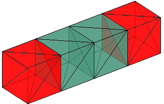
Figure 1: A depiction of the grasping experiment described in Section VII-A. The two red boxes act as grippers and push inward. Gravity pushes downward. Given sufficient friction ($\mu=\infty$), the grippers should ideally keep the blue boxes grasped using force closure.

This experiment yielded several findings. As expected, reducing the LCP variables by a factor of five (216 variables to 36 variables) results in much faster solutions ($451$–$558\%$ faster mean, depending on the solver). Fewer variables also results in less rounding error; the no-slip approach was able to model the grasping scenario reliably for at least 100 iterations (again, compared to around ten iterations for Stewart-Trinkle). Of the twelve contacts per pair of boxes, it was only necessary to apply forces to two contacts, which the modified PPM method was able to exploit: it ran nearly 20% faster than the quadprog algorithm (mean and maximum numbers of pivot operations were observed to be 5.5 and 7, respectively). This performance differential is considerable given that our modified PPM algorithm was not implemented as a MEX file and that our implementation does not use low-rank updates to maximize performance).

VII-B Locomotion experiments

We used the Moby simulator (https://github.com/PositronicsLab/Moby) to simulate a quadrupedal robot walking on a terrain map (see Figure 2) over ten seconds. An event-driven method (see [4] for a description of this paradigm) is used to simulate the system instead of the time-stepping approaches used in ODE, Bullet, and RPIsim; popular implementations of this approach are susceptible to energy gain when correcting interpenetration [21], which destabilizes our robot in the process.

The integration method used for the no-slip model experiment is symplectic Euler (Störmer-Verlet) with a step size of 0.001, while fourth-order Runge-Kutta integration was used for the viscous model experiment with identical step size. Our approach using the former integrator allows only the no-slip model to be activated, while our approach using the latter integrator permits the acceleration-level viscous model to be used for sustained contacts. When impacts occur (e.g., on initial foot/ground contact) in the latter approach, the simulation uses an inelastic impact model [7] with purely viscous friction.

Locomotion experiments were run on an Intel Xeon 2.27GHz desktop computer. All aspects of the simulation, including forward dynamics computations, collision detection, and controls (which performs dynamics calculations) were accounted for in results; single LCP solves generally run too quickly to obtain timings for just that operation. We point out that the simulations run considerably slower than similar systems modeled using, e.g., ODE, but the goals of the two simulators. ODE uses approximate solves and permits interpenetration. Moby aims to provide a verifiable simulator, i.e., one that adheres closely to the rigid body dynamics models (which means that interpenetration is impermissible).

Results for the no-slip experiment are provided in Table II, which shows a speedup of nearly 28%. The minimum and maximum number of contact points generated in the experiment is 1 and 30, respectively; the mean number of contact points is 6, and the standard deviation is 8. Thus, simulations with greater numbers of contacts could expect greater performance differentials.

Results for the viscous experiment are provided in Table III, which shows a speedup of over 37%. We note that the viscous friction experiments required significantly longer to run than the no-slip experiments. We hypothesize that this disparity is due to the behavior of the simulation when applying the viscous model, which tends to produce rapid movements upon contact. Those rapid movements, which appear due to some sensitivity in the underlying ordinary differential equations, slow the simulator’s continuous collision detection system (see [14] for a description of that system).

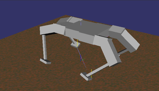
Figure 2: A depiction of the quadrupedal robot walking on a terrain map in the locomotion experiment, as described in Section VII-B. The no-slip and viscous friction models were both assessed.

Contact model	Running time
Drumwright-Shell	416.284s
$\mu_{c}=100.0,\mu_{v}=0.0$
No-slip (modified PPM)	301.796s

TABLE II: Times required to simulate the quadruped locomotion scenario described in Section VII-B under a no-slip contact model. Timings include all aspects of the simulation (including collision detection).

Contact model	Running time
Viscous (Lemke’s Algorithm)	2936.36s
$\mu_{c}=0.0,\mu_{v}=0.1$
Viscous (modified PPM)	2139.73s

TABLE III: Times required to simulate the quadruped locomotion scenario described in Section VII-B under a purely viscous friction model. Timings include all aspects of the simulation (including collision detection).

VIII Conclusion

We presented an algorithm for rapidly computing two rigid contact models without Coulomb friction that have proven useful in certain modeling and simulation applications for robotics. We showed how these models exhibit both asymptotic computational complexity and significant running time advantages over rigid models with Coulomb friction. While we do not expect these special-case models to replace rigid models with Coulomb friction, the former serve as computationally efficient alternatives as applications allow.

IX Acknowledgements

We thank Sam Zapolsky for providing the quadruped model and the locomotion controller. This work was funded by NSF CMMI-110532.

References

- [1] M. Anitescu and F. A. Potra. Formulating dynamic multi-rigid-body contact problems with friction as solvable linear complementarity problems. Nonlinear Dynamics, 14:231–247, 1997.
- [2] D. Baraff. Fast contact force computation for nonpenetrating rigid bodies. In Proc. of SIGGRAPH, Orlando, FL, July 1994.
- [3] R. Bhatia. Positive definite matrices. Princeton University Press, 2007.
- [4] B. Brogliato, A. A. ten Dam, L. Paoli, F. Génot, and S. Abadie. Numerical simulation of finite dimensional multibody nonsmooth mechanical systems. ASME Appl. Mech. Reviews, 55(2):107–150, March 2002.
- [5] R. W. Cottle. The principal pivoting method of quadratic programming. In G. Dantzig and J. A. F. Veinott, editors, Mathematics of Decision Sciences, pages 144–162. AMS, Rhode Island, 1968.
- [6] R. W. Cottle, J.-S. Pang, and R. Stone. The Linear Complementarity Problem. Academic Press, Boston, 1992.
- [7] E. Drumwright. Avoiding Zeno’s paradox in impulse-based rigid body simulation. In Proc. of IEEE Intl. Conf. on Robotics and Automation (ICRA), Anchorage, AK, 2010.
- [8] E. Drumwright and D. Shell. Extensive analysis of linear complementarity problem (LCP) solver performance on randomly generated rigid body contact problems. In Proc. IEEE/RSJ Intl. Conf. Intelligent Robots and Systems (IROS), Vilamoura, Algarve, Oct 2012.
- [9] P. L. Fackler and M. J. Miranda. LEMKE. http://people.sc.fsu.edu/ burkardt/m_src/lemke/lemke.m.
- [10] C. W. Kilmister and J. E. Reeve. Rational Mechanics. Longmans, London, 1966.
- [11] V. Klee and G. J. Minty. How good is the simplex algorithm? In Proc. of the Third Symp. on Inequalities, pages 159–175, UCLA, 1972.
- [12] C. E. Lemke. Bimatrix equilibrium points and mathematical programming. Management Science, 11:681–689, 1965.
- [13] K. Lynch and M. J. Mason. Pushing by slipping, slip with infinite friction, and perfectly rough surfaces. Intl. J. Robot. Res., 14(2):174–183, Apr 1995.
- [14] B. Mirtich. Impulse-based Dynamic Simulation of Rigid Body Systems. PhD thesis, University of California, Berkeley, 1996.
- [15] K. G. Murty. Linear Complementarity, Linear and Nonlinear Programming. Heldermann Verlag, Berlin, 1988.
- [16] P. Painlevé. Sur le lois du frottement de glissemment. C. R. Académie des Sciences Paris, 121:112–115, 1895.
- [17] L. Sciavicco and B. Siciliano. Modeling and Control of Robot Manipulators, 2nd Ed. Springer-Verlag, London, 2000.
- [18] R. Shamir. The efficiency of the simplex method: A survey. Management Science, 33(3):301–334, 1987.
- [19] R. Smith. ODE: Open Dynamics Engine.
- [20] D. A. Spielman and S.-H. Teng. Smoothed analysis: why the simplex algorithm usually takes polynomial time. J. of the ACM, 51(3):385–463, 2004.
- [21] D. Stewart and J. C. Trinkle. An implicit time-stepping scheme for rigid body dynamics with Coulomb friction. In Proc. of the IEEE Intl. Conf. on Robotics and Automation (ICRA), San Francisco, CA, April 2000.
- [22] D. E. Stewart. Rigid-body dynamics with friction and impact. SIAM Review, 42(1):3–39, Mar 2000.
- [23] D. E. Stewart and J. C. Trinkle. An implicit time-stepping scheme for rigid body dynamics with inelastic collisions and Coulomb friction. Intl. J. Numerical Methods in Engineering, 39(15):2673–2691, 1996.
- [24] J. Trinkle, J.-S. Pang, S. Sudarsky, and G. Lo. On dynamic multi-rigid-body contact problems with Coulomb friction. Zeithscrift fur Angewandte Mathematik und Mechanik, 77(4):267–279, 1997.
- [25] J. Wang. Dynamic grasp analysis and profiling of gazebo. Master’s thesis, Rennselaer Polytechnic Inst., 2013.